2.1 Non-dimensionalisation

For the sake of brevity, we present the model directly in dimensionless form and use the following scales:

(2.1) $$\begin{eqnarray}\left.\begin{array}{@{}c@{}}\displaystyle \boldsymbol{x}^{\ast }=L\boldsymbol{x},\quad (H^{\ast },h^{\ast })=L(H,h),\quad (\boldsymbol{u}^{\ast },\boldsymbol{U}^{\ast })=U_{\infty }(\boldsymbol{u},\boldsymbol{U}),\\ (p^{\ast },P^{\ast })=\unicode[STIX]{x1D70C}_{a}U_{\infty }^{2}(p,P),\quad (\unicode[STIX]{x1D703}^{\ast },\unicode[STIX]{x1D6E9}^{\ast },Q^{\ast })=T_{f}-(T_{\infty }-T_{f})(\unicode[STIX]{x1D703},\unicode[STIX]{x1D6E9},Q).\end{array}\right\}\end{eqnarray}$$

We may take $T_{f}>T_{\infty }$ without loss of generality and the above temperature scaling is purely for analytical convenience, since it fixes the film and ice temperatures on the ice surface at zero.

The above rescaling thus introduces the following dimensionless numbers into the model:

(2.2a-e ) $$\begin{eqnarray}Re=\frac{\unicode[STIX]{x1D70C}_{a}LU_{\infty }}{\unicode[STIX]{x1D707}_{a}},\quad We=\frac{\unicode[STIX]{x1D70C}_{a}LU_{\infty }^{2}}{\unicode[STIX]{x1D70E}},\quad Pr=\frac{\unicode[STIX]{x1D707}_{a}c_{a}}{\unicode[STIX]{x1D706}_{a}},\quad Pe_{i}=\frac{\unicode[STIX]{x1D70C}_{i}c_{i}LU_{\infty }}{\unicode[STIX]{x1D706}_{i}},\quad Ste=\frac{c_{i}(T_{f}-T_{\infty })}{{\mathcal{L}}},\end{eqnarray}$$

which are the air Reynolds, Weber and Prandtl numbers, the Péclet number in the ice and the Stefan number respectively; ${\mathcal{L}}$ denoting the latent heat of ice–water phase change. Furthermore, the air–water density, viscosity, thermal conductivity and specific heat ratios, and the water–ice density and thermal conductivity ratios are defined by

(2.3a-f ) $$\begin{eqnarray}\unicode[STIX]{x1D70C}=\frac{\unicode[STIX]{x1D70C}_{a}}{\unicode[STIX]{x1D70C}_{w}},\quad \unicode[STIX]{x1D707}=\frac{\unicode[STIX]{x1D707}_{a}}{\unicode[STIX]{x1D707}_{w}},\quad \unicode[STIX]{x1D706}=\frac{\unicode[STIX]{x1D706}_{a}}{\unicode[STIX]{x1D706}_{w}},\quad c=\frac{c_{a}}{c_{w}},\quad \hat{\unicode[STIX]{x1D70C}}=\frac{\unicode[STIX]{x1D70C}_{i}}{\unicode[STIX]{x1D70C}_{w}},\quad \hat{\unicode[STIX]{x1D706}}=\frac{\unicode[STIX]{x1D706}_{i}}{\unicode[STIX]{x1D706}_{w}}.\end{eqnarray}$$

In the course of this analysis, $\hat{\unicode[STIX]{x1D70C}}$ , $\hat{\unicode[STIX]{x1D706}}$ , $c$ and $Pr$ are assumed $O(1)$ , which is reasonable for air–water–ice systems – for example, when $T_{f}-T_{\infty }\approx 10~\text{K}$ , $\hat{\unicode[STIX]{x1D70C}}=0.9$ , $\hat{\unicode[STIX]{x1D706}}=4.11$ , $c=0.24$ , $Pr=0.69$ (cf. table 1 in § 6.1). However, we shall also assume that $\unicode[STIX]{x1D70C}$ , $\unicode[STIX]{x1D707}$ and $\unicode[STIX]{x1D706}$ are $O(1)$ , which are less reasonable assumptions for air–water–ice systems, although the assumption is not uncommon in the literature and it does not greatly affect the asymptotic structure, as discussed in § 6.1. Note that when $T_{f}-T_{\infty }\approx 10~\text{K}$ , $\unicode[STIX]{x1D70C}/\unicode[STIX]{x1D707}\approx 0.26$ , so that $Re=0.26Re_{w}$ , where $Re_{w}=\unicode[STIX]{x1D70C}_{w}LU_{\infty }/\unicode[STIX]{x1D707}_{w}$ is the Reynolds number in the liquid, so that throughout the analysis, we shall replace $Re_{w}$ by $\unicode[STIX]{x1D707}Re/\unicode[STIX]{x1D70C}$ where it would appear, and we assume that $Re_{w}=O(Re)$ .

Finally, we shall assume that the fluid properties are independent of the fluid temperature throughout the analysis, which decouples the flow and thermal problems in each phase. In general, this assumption would need to be checked carefully, since in an aircraft icing scenario, there can be a wide range of temperatures, from subzero external air flow to heating elements fed by excess bleed heat from the engines, which can be very high.

2.2 Dimensionless problem

The Navier–Stokes equations in each fluid are given by

(2.4) $$\begin{eqnarray}\displaystyle & \displaystyle u_{t}+uu_{x}+vu_{y}=-p_{x}+\frac{1}{Re}(u_{xx}+u_{yy}), & \displaystyle\end{eqnarray}$$

(2.5) $$\begin{eqnarray}\displaystyle & \displaystyle v_{t}+uv_{x}+vv_{y}=-p_{y}+\frac{1}{Re}(v_{xx}+v_{yy}), & \displaystyle\end{eqnarray}$$

(2.6) $$\begin{eqnarray}\displaystyle & \displaystyle u_{x}+v_{y}=0, & \displaystyle\end{eqnarray}$$

(2.7) $$\begin{eqnarray}\displaystyle & \displaystyle U_{t}+UU_{x}+VU_{y}=-\unicode[STIX]{x1D70C}P_{x}+\frac{\unicode[STIX]{x1D70C}}{\unicode[STIX]{x1D707}Re}(U_{xx}+U_{yy}), & \displaystyle\end{eqnarray}$$

(2.8) $$\begin{eqnarray}\displaystyle & \displaystyle V_{t}+UV_{x}+VU_{y}=-\unicode[STIX]{x1D70C}P_{y}+\frac{\unicode[STIX]{x1D70C}}{\unicode[STIX]{x1D707}Re}(V_{xx}+V_{yy}), & \displaystyle\end{eqnarray}$$

(2.9) $$\begin{eqnarray}\displaystyle & U_{x}+V_{y}=0. & \displaystyle\end{eqnarray}$$

On the plate, the no-slip, no-flux boundary conditions are given by

(2.10a,b ) $$\begin{eqnarray}U=0,\quad V=0\quad \text{on }y=0,\end{eqnarray}$$

while on the ice, the no-slip, no-flux conditions are

(2.11) $$\begin{eqnarray}(U,V)^{\text{T}}=(1-\hat{\unicode[STIX]{x1D70C}})h_{t}\boldsymbol{n}\quad \text{on }y=h,\end{eqnarray}$$

where $\boldsymbol{n}=(-h_{x},1)^{\text{T}}/(1+h_{x}^{2})^{1/2}$ is the outward unit normal to the ice surface. On the air–water interface, continuity of velocity and the kinematic condition must be satisfied, so that

(2.12a,b ) $$\begin{eqnarray}u=U,\quad v=V\quad \text{on }y=H,\end{eqnarray}$$

(2.13) $$\begin{eqnarray}V=H_{t}+UH_{x}\quad \text{on }y=H.\end{eqnarray}$$

Moreover, continuity of normal and tangential stress on the interface give

(2.14) $$\begin{eqnarray}\displaystyle p & = & \displaystyle P+\frac{H_{xx}}{We(1+H_{x}^{2})^{3/2}}+\frac{2}{Re(1+H_{x}^{2})}\left[H_{x}^{2}\left(u_{x}-\frac{U_{x}}{\unicode[STIX]{x1D707}}\right)\right.\nonumber\\ \displaystyle & & \displaystyle \left.+\,v_{y}-\frac{V_{y}}{\unicode[STIX]{x1D707}}-H_{x}\left(u_{y}+v_{x}-\frac{(U_{y}+V_{x})}{\unicode[STIX]{x1D707}}\right)\right]\quad \text{on }y=H,\end{eqnarray}$$

and

(2.15) $$\begin{eqnarray}\unicode[STIX]{x1D707}[2H_{x}(u_{x}-v_{y})+(H_{x}^{2}-1)(u_{y}+v_{x})]=2H_{x}(U_{x}-V_{y})+(H_{x}^{2}-1)(U_{y}+V_{x})\end{eqnarray}$$

on $y=H$ . These are supplemented with the far-field conditions

(2.16a,b ) $$\begin{eqnarray}u\rightarrow 1,\quad p\rightarrow 0\quad \text{as }x^{2}+y^{2}\rightarrow \infty .\end{eqnarray}$$

Similarly, the energy equations in each fluid and the heat equation in the ice are given by

(2.17) $$\begin{eqnarray}\displaystyle & \displaystyle \unicode[STIX]{x1D703}_{t}+u\unicode[STIX]{x1D703}_{x}+v\unicode[STIX]{x1D703}_{y}=\frac{1}{Pr\,Re}(\unicode[STIX]{x1D703}_{xx}+\unicode[STIX]{x1D703}_{yy}), & \displaystyle\end{eqnarray}$$

(2.18) $$\begin{eqnarray}\displaystyle & \displaystyle \unicode[STIX]{x1D6E9}_{t}+U\unicode[STIX]{x1D6E9}_{x}+V\unicode[STIX]{x1D6E9}_{y}=\frac{\unicode[STIX]{x1D70C}c}{\unicode[STIX]{x1D706}Pr\,Re}(\unicode[STIX]{x1D6E9}_{xx}+\unicode[STIX]{x1D6E9}_{yy}), & \displaystyle\end{eqnarray}$$

(2.19) $$\begin{eqnarray}\displaystyle & \displaystyle Q_{t}=\frac{1}{Pe_{i}}(Q_{xx}+Q_{yy}), & \displaystyle\end{eqnarray}$$

respectively. We discuss the plate temperature profile, $T_{wall}(x,t)$ , in § 2.3, but will give the appropriate boundary conditions on the non-iced and iced regions here. On the non-iced part of the plate, the film temperature must satisfy

(2.20) $$\begin{eqnarray}\unicode[STIX]{x1D6E9}=T_{wall}(x,t),\end{eqnarray}$$

while on the iced part of the plate, we naturally have

(2.21) $$\begin{eqnarray}Q=T_{wall}(x,t).\end{eqnarray}$$

Continuity of temperature and continuity of heat flux across the free surface of the film are given by

(2.22a,b ) $$\begin{eqnarray}\unicode[STIX]{x1D703}=\unicode[STIX]{x1D6E9},\quad \unicode[STIX]{x1D706}(\unicode[STIX]{x1D703}_{y}-H_{x}\unicode[STIX]{x1D703}_{x})=\unicode[STIX]{x1D6E9}_{y}-H_{x}\unicode[STIX]{x1D6E9}_{x}\quad \text{on }y=H.\end{eqnarray}$$

On the ice surface, we must have

(2.23) $$\begin{eqnarray}\unicode[STIX]{x1D6E9}(x,h,t)=Q(x,h,t)=0,\end{eqnarray}$$

while the Stefan condition is given by

(2.24) $$\begin{eqnarray}\frac{Pe_{i}}{Ste}h_{t}=Q_{y}-h_{x}Q_{x}-\frac{1}{\hat{\unicode[STIX]{x1D706}}}(\unicode[STIX]{x1D6E9}_{y}-h_{x}\unicode[STIX]{x1D6E9}_{x})\quad \text{on }y=h.\end{eqnarray}$$

Finally, the far-field condition is

(2.25) $$\begin{eqnarray}\unicode[STIX]{x1D703}\rightarrow -1\quad \text{as }x^{2}+y^{2}\rightarrow \infty .\end{eqnarray}$$

2.3 The plate temperature condition

At time $t=0^{-}$ the plate is held at a constant temperature $\unicode[STIX]{x1D6FD}\,=\,(T_{w}-T_{f})/(T_{f}-T_{\infty })\,>\,0$ , at which point the plate heating is switched off for $x>x_{0}$ , where $x_{0}=O(1)$ . It transpires that the small-time response of the flow to temperature change has a major role on the long-time film dynamics. For this reason, we consider a wall boundary condition that is continuous in time. Therefore, we set

(2.26) $$\begin{eqnarray}T_{wall}(x,t)=\left\{\begin{array}{@{}ll@{}}\unicode[STIX]{x1D6FD}\quad & \text{for }x<x_{0},\\ \displaystyle \unicode[STIX]{x1D6FD}-(\unicode[STIX]{x1D6FD}+\unicode[STIX]{x1D6FC})f\left(\frac{t}{\unicode[STIX]{x1D70F}}\right)\quad & \text{for }x>x_{0},\end{array}\right.\end{eqnarray}$$

where $\unicode[STIX]{x1D6FC}=(T_{f}-T_{cold})/(T_{f}-T_{\infty })>0$ , $T_{cold}<T_{f}$ is specified, $\unicode[STIX]{x1D70F}\gg 1$ and the function $f$ is such that $f(0)=0$ and $f\rightarrow 1$ as $t\rightarrow \infty$ for all $x>x_{0}$ . Assuming that $f$ is continuous and monotonic in time, there is a time $t=\unicode[STIX]{x1D70F}t_{c}$ with $t_{c}=O(1)$ at which ice first begins to form – corresponding to the first time at which the plate temperature reaches the freezing temperature for $x>x_{0}$ . Though we have chosen a step profile for the plate temperature here, it is relatively straightforward to generalise to continuous profiles, which give a more physical representation of the plate temperature distribution, although the horizontal location of the ice front is a function of time in such instances.

As seen in the definition of $T_{wall}$ , equation (2.26), the cooling of the plate happens over a long time scale, $\unicode[STIX]{x1D70F}\gg 1$ . This means that the flow is quasi-steady and temporal effects arise in the ice growth and the film evolution. Thus, there are three distinct temporal regimes in the switch-off problem:

1. (i) when $0<t<\unicode[STIX]{x1D70F}t_{c}$ , there is no ice growth, the flow is steady and the thermal problem accounts for the change in plate condition;

2. (ii) when $t>\unicode[STIX]{x1D70F}t_{c}$ , $t-\unicode[STIX]{x1D70F}t_{c}=O(1)$ , there is ice growth, but the magnitude of the temperature jump across the ice layer is small;

3. (iii) when $t>\unicode[STIX]{x1D70F}t_{c}$ , $t-\unicode[STIX]{x1D70F}t_{c}=O(\unicode[STIX]{x1D70F})$ , the temperature jump across the ice layer is of order unity.

We shall discuss each of these regimes separately in §§ 3, 4 and 5 respectively.

3.1 The flow problem

The flow problem decouples from the thermal problem and hence remains steady. We expand variables in asymptotic series of the form (recall $\unicode[STIX]{x1D700}_{w}Re^{1/2}\ll 1$ )

(3.4) $$\begin{eqnarray}\hat{u} =\hat{u} _{0}+\unicode[STIX]{x1D700}_{w}Re^{1/2}\hat{u} _{1}+\unicode[STIX]{x1D700}_{w}^{2}Re\,\hat{u} _{2}+\cdots \,.\end{eqnarray}$$

To leading order,

(3.5a-c ) $$\begin{eqnarray}\hat{u} _{0}=F^{\prime }\left(\frac{{\hat{y}}}{\sqrt{x}}\right),\quad \hat{v}_{0}=\frac{-1}{2\sqrt{x}}\left(F\left(\frac{{\hat{y}}}{\sqrt{x}}\right)-\frac{{\hat{y}}}{\sqrt{x}}F^{\prime }\left(\frac{{\hat{y}}}{\sqrt{x}}\right)\right),\quad \hat{p}_{0}=0\end{eqnarray}$$

in the air, where $F$ satisfies Blasius’s equation

(3.6a-c ) $$\begin{eqnarray}F^{\prime \prime \prime }+\frac{FF^{\prime \prime }}{2}=0,\quad F(0)=F^{\prime }(0)=0,\quad F^{\prime }(\infty )=1.\end{eqnarray}$$

In particular, note that 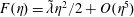$F(\unicode[STIX]{x1D702})=\tilde{\unicode[STIX]{x1D706}}\unicode[STIX]{x1D702}^{2}/2+O(\unicode[STIX]{x1D702}^{5})$ as $\unicode[STIX]{x1D702}\rightarrow 0^{+}$ , where $\tilde{\unicode[STIX]{x1D706}}=0.332$ . In the film, the leading-order problem is given by

(3.7a-c ) $$\begin{eqnarray}\hat{U} _{0\bar{y}\bar{y}}=0,\quad \hat{P}_{0\bar{y}}=0,\quad \hat{U} _{0x}+\hat{V}_{0\bar{y}}=0,\end{eqnarray}$$

such that

(3.8a-d ) $$\begin{eqnarray}\hat{U} _{0}(x,0)=0,\quad \hat{V}_{0}(x,0)=0,\quad \hat{U} _{0\bar{y}}(x,{\hat{H}}_{0})=\unicode[STIX]{x1D707}\hat{u} _{0{\hat{y}}}(x,0),\quad \hat{P}_{0}(x,0)=0.\end{eqnarray}$$

Therefore, it is straightforward to show that

(3.9a-d ) $$\begin{eqnarray}\hat{U} _{0}=\frac{\tilde{\unicode[STIX]{x1D706}}\unicode[STIX]{x1D707}\bar{y}}{\sqrt{x}},\quad \hat{V}_{0}=\frac{\tilde{\unicode[STIX]{x1D706}}\unicode[STIX]{x1D707}\bar{y}^{2}}{4x^{3/2}},\quad \hat{P}_{0}=0,\quad {\hat{H}}_{0}={\mathcal{A}}_{0}x^{1/4},\end{eqnarray}$$

where ${\mathcal{A}}_{0}$ is a constant determined by prescribing the flux of fluid at $x=0$ .

At $O(\unicode[STIX]{x1D700}_{w}Re^{1/2})$ , the correction to the Blasius solution in the air satisfies

(3.10a-c ) $$\begin{eqnarray}(\hat{u} _{0}\hat{u} _{1})_{x}+\hat{v}_{0}\hat{u} _{1{\hat{y}}}+\hat{v}_{1}\hat{u} _{0{\hat{y}}}=-\hat{p}_{1x}+\hat{u} _{1{\hat{y}}{\hat{y}}},\quad 0=-\hat{p}_{1{\hat{y}}},\quad \hat{u} _{1x}+\hat{v}_{1{\hat{y}}}=0,\end{eqnarray}$$

subject to

(3.11a,b ) $$\begin{eqnarray}\hat{u} _{1}(x,0)=\frac{\tilde{\unicode[STIX]{x1D706}}(\unicode[STIX]{x1D707}-1){\hat{H}}_{0}}{\sqrt{x}},\quad \hat{v}_{1}(x,0)=0,\end{eqnarray}$$

while at infinity, we require

(3.12a,b ) $$\begin{eqnarray}\hat{u} _{1}\rightarrow 0,\quad \hat{p}_{1}\rightarrow 0\quad \text{as }{\hat{y}}\rightarrow \infty .\end{eqnarray}$$

Hence $\hat{p}_{1}=0$ , and we typically have to solve for $\hat{u} _{1}$ , $\hat{v}_{1}$ numerically, which we do not pursue here. In the film, the $O(\unicode[STIX]{x1D700}_{w}Re^{1/2})$ -correction to the flow solution is given by

(3.13a-d ) $$\begin{eqnarray}\hat{U} _{1}=\unicode[STIX]{x1D707}\hat{u} _{1{\hat{y}}}(x,0)\bar{y},\quad \hat{V}_{1}=\frac{-\unicode[STIX]{x1D707}\hat{u} _{1x{\hat{y}}}(x,0)\bar{y}^{2}}{2},\quad \hat{P}_{1}=0,\quad {\hat{H}}_{1}=\frac{{\mathcal{A}}_{1}x^{1/4}}{{\mathcal{A}}_{0}\tilde{\unicode[STIX]{x1D706}}}-\frac{\hat{u} _{1{\hat{y}}}(x,0){\mathcal{A}}_{0}x^{3/4}}{2\tilde{\unicode[STIX]{x1D706}}},\end{eqnarray}$$

where in the $O(\unicode[STIX]{x1D700}_{w}Re^{1/2})$ -form of the shear stress condition, we have used the fact that the second derivative of the Blasius solution vanishes on the plate, that is $\hat{u} _{0{\hat{y}}{\hat{y}}}(x,0)=0$ . The constant ${\mathcal{A}}_{1}$ is the $O(\unicode[STIX]{x1D700}_{w}Re^{1/2})$ -correction to the flux of fluid at the plate tip.

3.2 The thermal problem

To leading order, the thermal problem is given by

(3.14) $$\begin{eqnarray}\displaystyle & \displaystyle \hat{u} _{0}\hat{\unicode[STIX]{x1D703}}_{0x}+\hat{v}_{0}\hat{\unicode[STIX]{x1D703}}_{0{\hat{y}}}=\frac{1}{Pr}\hat{\unicode[STIX]{x1D703}}_{0{\hat{y}}{\hat{y}}}, & \displaystyle\end{eqnarray}$$

(3.15) $$\begin{eqnarray}\displaystyle & \displaystyle 0=\frac{\unicode[STIX]{x1D70C}c}{\unicode[STIX]{x1D706}Pr}\hat{\unicode[STIX]{x1D6E9}}_{0\bar{y}\bar{y}}, & \displaystyle\end{eqnarray}$$

such that

(3.16a-d ) $$\begin{eqnarray}\hat{\unicode[STIX]{x1D6E9}}_{0}(x,0)=T_{wall}(\bar{t}),\quad \hat{\unicode[STIX]{x1D703}}_{0}(x,0)=\hat{\unicode[STIX]{x1D6E9}}_{0}(x,{\hat{H}}_{0}),\quad \hat{\unicode[STIX]{x1D6E9}}_{0\bar{y}}(x,{\hat{H}}_{0})=0,\quad \hat{\unicode[STIX]{x1D703}}_{0}\rightarrow -1\quad \text{as }{\hat{y}}\rightarrow \infty .\end{eqnarray}$$

Therefore, it is straightforward to show that the film temperature is constant across the layer, with

(3.17) $$\begin{eqnarray}\hat{\unicode[STIX]{x1D6E9}}_{0}=\left\{\begin{array}{@{}ll@{}}\unicode[STIX]{x1D6FD}\quad & \text{for }y=0,x<x_{0},\\ \unicode[STIX]{x1D6FD}-(\unicode[STIX]{x1D6FD}+\unicode[STIX]{x1D6FC})f(\bar{t})\quad & \text{for }y=0,x>x_{0}.\end{array}\right.\end{eqnarray}$$

The leading-order film temperature acts as a Dirichlet condition for the leading-order problem for air temperature. To solve this problem, we note that if we consider a problem in which $\unicode[STIX]{x1D703}_{b}$ satisfies (3.14) subject to

(3.18a,b ) $$\begin{eqnarray}\unicode[STIX]{x1D703}_{b}(x,0,\bar{t})=\unicode[STIX]{x1D6FD},\quad \unicode[STIX]{x1D703}_{b}\rightarrow -1\quad \text{as}\;{\hat{y}}\rightarrow \infty ,\end{eqnarray}$$

we can use the Blasius similarity variable, $\unicode[STIX]{x1D702}={\hat{y}}/\sqrt{x}$ , to integrate (3.14) and we deduce that $\unicode[STIX]{x1D703}_{b}=\unicode[STIX]{x1D6FD}-(1+\unicode[STIX]{x1D6FD})G(\unicode[STIX]{x1D702})$ , where

(3.19) $$\begin{eqnarray}G(\unicode[STIX]{x1D702})=\frac{\displaystyle \int _{0}^{\unicode[STIX]{x1D702}}\text{exp}\left(-\frac{Pr}{2}\int _{0}^{s}F(\unicode[STIX]{x1D70F})\,\text{d}\unicode[STIX]{x1D70F}\right)\,\text{d}s}{\displaystyle \int _{0}^{\infty }\text{exp}\left(-\frac{Pr}{2}\int _{0}^{s}F(\unicode[STIX]{x1D70F})\,\text{d}\unicode[STIX]{x1D70F}\right)\,\text{d}s}.\end{eqnarray}$$

Clearly, $\hat{\unicode[STIX]{x1D703}}_{0}=\unicode[STIX]{x1D703}_{b}$ is the solution for all $0<\bar{t}<t_{c}$ for $x<x_{0}$ . For $x>x_{0}$ , we write $\hat{\unicode[STIX]{x1D703}}_{0}=\unicode[STIX]{x1D703}_{b}(x,{\hat{y}})+\tilde{\unicode[STIX]{x1D703}}(x,{\hat{y}},\bar{t})$ and make use of the Lighthill approximation, which assumes that the perturbation to the steady-state solution due to the change in the plate temperature is confined to a sublayer of the thermal boundary layer in which $u_{0}$ and $v_{0}$ are well approximated by their shear profiles for small ${\hat{y}}$ , see Lighthill (Reference Lighthill1950) and Higuera (Reference Higuera1991). In the appendix A, we show that the Lighthill approximation is reasonable by computing the full solutions and comparing with the approximation. Thus, the velocity components are approximated by

(3.20a,b ) $$\begin{eqnarray}\hat{u} _{0}\sim \frac{\tilde{\unicode[STIX]{x1D706}}{\hat{y}}}{\sqrt{x}},\quad \hat{v}_{0}\sim \frac{\tilde{\unicode[STIX]{x1D706}}{\hat{y}}^{2}}{4x^{3/4}},\end{eqnarray}$$

so that

(3.21) $$\begin{eqnarray}\frac{\tilde{\unicode[STIX]{x1D706}}{\hat{y}}}{\sqrt{x}}\tilde{\unicode[STIX]{x1D703}}_{x}+\frac{\tilde{\unicode[STIX]{x1D706}}{\hat{y}}^{2}}{4x^{3/4}}\tilde{\unicode[STIX]{x1D703}}_{{\hat{y}}}=\frac{\tilde{\unicode[STIX]{x1D703}}_{{\hat{y}}{\hat{y}}}}{Pr},\end{eqnarray}$$

subject to

(3.22a,b ) $$\begin{eqnarray}\tilde{\unicode[STIX]{x1D703}}(x,0,\bar{t})=-(\unicode[STIX]{x1D6FD}+\unicode[STIX]{x1D6FC})f(\bar{t}),\quad \tilde{\unicode[STIX]{x1D703}}\rightarrow 0\quad \text{as }{\hat{y}}\rightarrow \infty .\end{eqnarray}$$

We can solve (3.21) and (3.22) explicitly by seeking a similarity solution of the form $\tilde{\unicode[STIX]{x1D703}}=L(\unicode[STIX]{x1D701},\bar{t})$ , $\unicode[STIX]{x1D701}={\hat{y}}/d(x)$ and find that

(3.23) $$\begin{eqnarray}\displaystyle & \displaystyle d(x)=\left(\frac{4}{\tilde{\unicode[STIX]{x1D706}}Pr}\right)^{1/3}x^{1/4}(x^{3/4}-x_{0}^{3/4})^{1/3}, & \displaystyle\end{eqnarray}$$

(3.24) $$\begin{eqnarray}\displaystyle & \displaystyle L(\unicode[STIX]{x1D701},\bar{t})=-(\unicode[STIX]{x1D6FD}+\unicode[STIX]{x1D6FC})f(\bar{t})\left(1-\frac{3^{2/3}}{\unicode[STIX]{x1D6E4}(1/3)}\int _{0}^{\unicode[STIX]{x1D701}}\text{e}^{-s^{3}/3}\,\text{d}s\right). & \displaystyle\end{eqnarray}$$

The behaviour of $d(x)$ – which essentially represents the size of the region where the change to the steady-state temperature profile is appreciable – as $x\rightarrow x_{0}^{+}$ is given by

(3.25) $$\begin{eqnarray}d(x)\sim \left(\frac{3x_{0}^{1/2}}{\tilde{\unicode[STIX]{x1D706}}Pr}\right)^{1/3}(x-x_{0})^{1/3}+\cdots \quad \text{as }x\rightarrow x_{0}^{+}.\end{eqnarray}$$

Proceeding to $O(\unicode[STIX]{x1D700}_{w}Re^{1/2})$ in the film, we find that

(3.26) $$\begin{eqnarray}\hat{\unicode[STIX]{x1D6E9}}_{1}=\left\{\begin{array}{@{}ll@{}}\displaystyle -\frac{\unicode[STIX]{x1D706}(1+\unicode[STIX]{x1D6FD})G^{\prime }(0)\bar{y}}{\sqrt{x}}\quad & \text{for }x<x_{0},\\ \displaystyle \left[-\frac{\unicode[STIX]{x1D706}(1+\unicode[STIX]{x1D6FD})G^{\prime }(0)}{\sqrt{x}}+\frac{3^{2/3}\unicode[STIX]{x1D706}(\unicode[STIX]{x1D6FD}+\unicode[STIX]{x1D6FC})f(\bar{t})}{\unicode[STIX]{x1D6E4}(1/3)d(x)}\right]\bar{y}\quad & \text{for }x>x_{0}.\end{array}\right.\end{eqnarray}$$

Now, since $1/d(x)$ is singular at the switch-off point, cf. (3.25), clearly the $O(\unicode[STIX]{x1D700}_{w}Re^{1/2})$ -correction for $\hat{\unicode[STIX]{x1D6E9}}$ is singular at $x=x_{0}$ . Therefore, there is an inner region centred around $x=x_{0}$ in which the air and film thermal problems are coupled at leading order and the expressions used for the velocities in the Lighthill approximation have to be amended to account for the $O(\unicode[STIX]{x1D700}_{w}Re^{1/2})$ -terms in the velocity expansion. This inner region has horizontal extent of $O(\unicode[STIX]{x1D700}_{w}^{3}Re^{3/2})$ and thickness $O(\unicode[STIX]{x1D700}_{w})$ . However, before freezing, the inner region does not contribute anything significant to the analysis, so we shall forgo looking at it until § 4.3.

Thus, we have described how each fluid changes from the steady state once the plate cooling is introduced. Specifically, the flow remains unchanged from the Nelson et al. (Reference Nelson, Alving and Joseph1995) steady state discussed in § 3.1, while the temperature in each fluid decreases due to the cooling effect of the plate for $x>x_{0}$ . Due to the nature of our problem configuration, there is a singularity in the air and film temperature profiles close to the switch-off point $x=x_{0}$ , which will need further investigation once ice growth begins.

4.1 Asymptotic structure

The asymptotic structure is pictured in figure 2. Away from the switch-off point in regions Ia–c upstream (i.e. for $x<x_{0}$ ), the air and the film do not undergo any change from their steady-state solutions at leading order and we expect the scalings of §§ 3.1 and 3.2 to hold there. Furthermore, under the assumptions made on the size of the ice growth and the thickness of the ice, the air and film should also evolve on the steady-state scales downstream. In the outer ice region Ic, there is an $O(1/\unicode[STIX]{x1D70F})$ -jump in the temperature over a vertical distance of size $\unicode[STIX]{x1D700}_{i}$ .

Close to the switch-off point, we expect there to be a slightly different behaviour caused by the sudden change in morphology due to the presence of the ice. Indeed, as alluded to in § 3.2, our outer analysis in § 4.2 breaks down when $x-x_{0}=O(\unicode[STIX]{x1D700}_{w}^{3}Re^{3/2})$ and $y=O(\unicode[STIX]{x1D700}_{w})$ in the air, so there is an inner problem to consider on this scale, denoted by regions IIIa–c. In the inner region, the air and film flows are coupled at leading order. We assume that $\unicode[STIX]{x1D700}_{w}^{3}Re^{3/2}\gg \unicode[STIX]{x1D700}_{w}$ , so that the inner region still has a long, thin aspect ratio. Therefore, there is in fact a further ‘inner–inner’ region in which $x-x_{0}\sim \unicode[STIX]{x1D700}_{w}$ and the quasi-steady Navier–Stokes equations hold. We do not consider the inner–inner region in any detail in this paper.

It transpires that the free surface solutions in the inner and outer regions do not match, so we need an additional intermediate region between the inner and the downstream outer in which $x-x_{0}=O(\unicode[STIX]{x1D700}_{w}Re^{1/2})$ and $y=O(\unicode[STIX]{x1D700}_{w})$ . We denote the air, film and ice parts of this region by IIa–c respectively. In this region, the flow and temperature solutions are essentially local forms of the outer solution, but the equation describing the evolution of the free surface is hyperbolic.

Figure 2. Asymptotic structure of the switch-off problem for $T=O(1)$ as described in the text: the outer regions Ia–c, the intermediate regions IIa–c and the inner regions IIIa–c, where a, b, c correspond to the air, film and ice respectively.

4.2 Outer region

For the sake of brevity we define $h\equiv 0$ for $x<x_{0}$ . The scalings for the outer regions Ia–c are given by (3.1) and (3.2), along with the time scale (4.1) and the ice layer scalings

(4.5a-c ) $$\begin{eqnarray}y=\unicode[STIX]{x1D700}_{w}^{2}Re^{1/2}Y,\quad h=\unicode[STIX]{x1D700}_{w}^{2}Re^{1/2}{\hat{h}},\quad Q=\unicode[STIX]{x1D700}_{w}Re^{1/2}\hat{Q}.\end{eqnarray}$$

We note in particular that the horizontal coordinates in the air, film and ice regions are denoted by ${\hat{y}}$ , $\bar{y}$ and $Y$ respectively. After substituting these into (2.4)–(2.25), we return the same problem as in § 3 with $\unicode[STIX]{x1D70F}=1$ , which brings in the time derivatives in the leading-order momentum and energy equations in the air; with the no-slip, no-flux conditions on the ice surface replaced by

(4.6a,b ) $$\begin{eqnarray}\hat{U} +\unicode[STIX]{x1D700}_{w}^{3}Re^{1/2}{\hat{h}}_{x}\hat{V}=0,\quad \hat{V}=(1-\hat{\unicode[STIX]{x1D70C}}){\hat{h}}_{T}\quad \text{on }\bar{y}=\unicode[STIX]{x1D700}_{w}Re^{1/2}{\hat{h}},\end{eqnarray}$$

and, recalling that $\unicode[STIX]{x1D70F}=1/\unicode[STIX]{x1D700}_{w}Re^{1/2}$ , the plate temperature condition is given by

(4.7) $$\begin{eqnarray}\left.\begin{array}{@{}ll@{}}\displaystyle \hat{\unicode[STIX]{x1D6E9}}(x,0,T)=\unicode[STIX]{x1D6FD} & \text{for }x<x_{0},\\ \displaystyle \hat{Q}(x,0,T)=-(\unicode[STIX]{x1D6FD}+\unicode[STIX]{x1D6FC})\left(f^{\prime }(t_{c})T+\unicode[STIX]{x1D700}_{w}Re^{1/2}\frac{f^{\prime \prime }(t_{c})T^{2}}{2}+\cdots \right) & \text{for }x>x_{0}.\end{array}\right\}\end{eqnarray}$$

Additionally, the energy equation in the ice (2.19) becomes

(4.8) $$\begin{eqnarray}\unicode[STIX]{x1D700}_{w}^{4}Re\,Pe_{i}\,\hat{Q}_{T}=\unicode[STIX]{x1D700}_{w}^{4}Re\,\hat{Q}_{xx}+\hat{Q}_{YY},\end{eqnarray}$$

and we also require the temperature and Stefan conditions on the ice surface (2.23)–(2.24), which are given by

(4.9a,b ) $$\begin{eqnarray}\hat{\unicode[STIX]{x1D6E9}}(x,\unicode[STIX]{x1D700}_{w}Re^{1/2}{\hat{h}},T)=0,\quad \hat{Q}(x,{\hat{h}},T)=0,\end{eqnarray}$$

and

(4.10) $$\begin{eqnarray}{\hat{h}}_{T}=(\hat{Q}_{Y}-\unicode[STIX]{x1D700}_{w}^{4}Re\,{\hat{h}}_{x}\hat{Q}_{x})|_{Y={\hat{h}}}-\frac{1}{\hat{\unicode[STIX]{x1D706}}}(\hat{\unicode[STIX]{x1D6E9}}_{\bar{y}}-\unicode[STIX]{x1D700}_{w}^{3}Re^{1/2}{\hat{h}}_{x}\hat{\unicode[STIX]{x1D6E9}}_{x})|_{\bar{y}=\unicode[STIX]{x1D700}_{w}Re^{1/2}{\hat{h}}}\end{eqnarray}$$

respectively.

4.2.1 Outer flow problem

Treating ${\hat{h}}$ as a known quantity, the flow problem decouples from the thermal problem, as in § 3.1. With the exception of the free surface profile, each of the variables is expanded as an asymptotic series of the form

(4.11) $$\begin{eqnarray}\hat{u} =\hat{u} _{0}+\unicode[STIX]{x1D700}_{w}Re^{1/2}\hat{u} _{1}+\unicode[STIX]{x1D700}_{w}^{2}Re\,\hat{u} _{2}+\cdots \,.\end{eqnarray}$$

For the free surface profile, since the coefficient of ${\hat{H}}_{T}$ in the kinematic boundary condition is large (cf. (2.13)), we need to write $H$ as a perturbation to the leading-order steady-state free surface profile: this is not surprising, since the ice is much thinner than the film, we do not expect the change to the steady-state film thickness to be of order unity. Hence, we write

(4.12) $$\begin{eqnarray}{\hat{H}}={\mathcal{A}}_{0}x^{1/4}+\unicode[STIX]{x1D700}_{w}Re^{1/2}{\hat{H}}_{0}+\unicode[STIX]{x1D700}_{w}^{2}Re\,{\hat{H}}_{1}+\cdots \,.\end{eqnarray}$$

At leading order, the steady solution prevails in the air, so that $\hat{u} _{0}$ , $\hat{v}_{0}$ and $\hat{p}_{0}$ are given by (3.5). In the film, the leading-order flow is still given by (3.9), but with the vertical component of velocity altered to take account of the ice growth through (4.6), so that

(4.13) $$\begin{eqnarray}\hat{V}_{0}=\frac{\tilde{\unicode[STIX]{x1D706}}\unicode[STIX]{x1D707}\bar{y}^{2}}{4x^{3/2}}+(1-\hat{\unicode[STIX]{x1D70C}}){\hat{h}}_{0T}.\end{eqnarray}$$

Substituting $\hat{U} _{0}$ and $\hat{V}_{0}$ into the leading-order form of (2.13), integrating and applying the initial condition given in (3.13), we find that

(4.14) $$\begin{eqnarray}{\hat{H}}_{0}=(1-\hat{\unicode[STIX]{x1D70C}}){\hat{h}}_{0}+\frac{{\mathcal{A}}_{1}x^{1/4}}{{\mathcal{A}}_{0}\tilde{\unicode[STIX]{x1D706}}}-\frac{\hat{u} _{1{\hat{y}}}(x,0){\mathcal{A}}_{0}x^{3/4}}{2\tilde{\unicode[STIX]{x1D706}}}.\end{eqnarray}$$

For convenience, we shall define

(4.15) $$\begin{eqnarray}H_{s1}(x)=\frac{{\mathcal{A}}_{1}x^{1/4}}{{\mathcal{A}}_{0}\tilde{\unicode[STIX]{x1D706}}}-\frac{\hat{u} _{1{\hat{y}}}(x,0){\mathcal{A}}_{0}x^{3/4}}{2\tilde{\unicode[STIX]{x1D706}}},\end{eqnarray}$$

henceforth. Therefore, defining ${\hat{H}}_{0}-{\hat{h}}_{0}$ as the leading-order correction to the steady-state film thickness, we see that the film thickness in the outer region decreases uniformly according to the amount of fluid lost to the ice layer.

We do not seek to solve the flow problems at $O(\unicode[STIX]{x1D700}_{w}Re^{1/2})$ and $O(\unicode[STIX]{x1D700}_{w}^{2}Re)$ in detail, but for future reference, we do note that the first- and second-order slip conditions felt by the air layer are given by

(4.16) $$\begin{eqnarray}\left.\begin{array}{@{}c@{}}\displaystyle \hat{u} _{1}(x,0)=\frac{\tilde{\unicode[STIX]{x1D706}}}{\sqrt{x}}(\unicode[STIX]{x1D707}-1){\mathcal{A}}_{0}x^{1/4},\\ \displaystyle \hat{u} _{2}(x,0,T)=\hat{u} _{1{\hat{y}}}(x,0){\mathcal{A}}_{0}(\unicode[STIX]{x1D707}-1)x^{1/4}+\frac{\tilde{\unicode[STIX]{x1D706}}}{\sqrt{x}}(\unicode[STIX]{x1D707}-1){\hat{H}}_{0}-\frac{\tilde{\unicode[STIX]{x1D706}}\unicode[STIX]{x1D707}{\hat{h}}_{0}}{\sqrt{x}},\end{array}\right\}\end{eqnarray}$$

and that the first-order correction to the horizontal component of the film velocity is

(4.17) $$\begin{eqnarray}\hat{U} _{1}=\unicode[STIX]{x1D707}\hat{u} _{1{\hat{y}}}(x,0)\bar{y}-\frac{\tilde{\unicode[STIX]{x1D706}}\unicode[STIX]{x1D707}{\hat{h}}_{0}}{\sqrt{x}}.\end{eqnarray}$$

4.2.2 Outer thermal problem

The leading-order thermal problem is very similar to the before freezing problem in § 3.2. To leading-order, the film temperature does not vary across the layer, so that

(4.18) $$\begin{eqnarray}\hat{\unicode[STIX]{x1D6E9}}_{0}=\left\{\begin{array}{@{}ll@{}}\unicode[STIX]{x1D6FD}\quad & \text{for }x<x_{0},\\ 0\quad & \text{for }x>x_{0}.\end{array}\right.\end{eqnarray}$$

Therefore, the leading-order air temperature must satisfy

(4.19) $$\begin{eqnarray}\hat{\unicode[STIX]{x1D703}}_{0T}+u_{b}\hat{\unicode[STIX]{x1D703}}_{0x}+v_{b}\hat{\unicode[STIX]{x1D703}}_{0{\hat{y}}}=\frac{\hat{\unicode[STIX]{x1D703}}_{0{\hat{y}}{\hat{y}}}}{Pr},\end{eqnarray}$$

subject to

(4.20a,b ) $$\begin{eqnarray}\hat{\unicode[STIX]{x1D703}}_{0}=\hat{\unicode[STIX]{x1D6E9}}_{0}\quad \text{on }{\hat{y}}=0,\quad \hat{\unicode[STIX]{x1D703}}_{0}\rightarrow -1\quad \text{as }{\hat{y}}\rightarrow \infty ,\end{eqnarray}$$

with the initial condition

(4.21) $$\begin{eqnarray}\hat{\unicode[STIX]{x1D703}}_{0}(x,{\hat{y}},0)=\left\{\begin{array}{@{}ll@{}}\unicode[STIX]{x1D703}_{b}(x,{\hat{y}})\quad & \text{for }x<x_{0},\\ \displaystyle \unicode[STIX]{x1D703}_{b}(x,{\hat{y}})+L\left({\hat{y}}/d(x),t_{c}\right)\quad & \text{for }x>x_{0}.\end{array}\right.\end{eqnarray}$$

It is straightforward that to show the initial condition satisfies (4.19) and (4.20) exactly for all $T>0$ .

Assuming that $\unicode[STIX]{x1D700}_{w}^{4}Re\,Pe_{i}\ll 1$ , by (4.8), the leading-order ice temperature profile varies only linearly across the layer, so that applying (4.7) and (4.9), we find that

(4.22) $$\begin{eqnarray}\hat{Q}_{0}=-(\unicode[STIX]{x1D6FD}+\unicode[STIX]{x1D6FC})f^{\prime }(t_{c})T\left(1-\frac{Y}{{\hat{h}}_{0}}\right).\end{eqnarray}$$

Hence, using the leading-order form of the Stefan condition, (4.10) along with the initial condition, ${\hat{h}}_{0}=0$ , we find that

(4.23) $$\begin{eqnarray}{\hat{h}}_{0}=\sqrt{(\unicode[STIX]{x1D6FD}+\unicode[STIX]{x1D6FC})f^{\prime }(t_{c})}T.\end{eqnarray}$$

At $O(\unicode[STIX]{x1D700}_{w}Re^{1/2})$ , the correction to the film temperature is driven purely by the heat flux from the air. We find that

(4.24) $$\begin{eqnarray}\hat{\unicode[STIX]{x1D6E9}}_{1}=\left\{\begin{array}{@{}ll@{}}\displaystyle -\frac{\unicode[STIX]{x1D706}(1+\unicode[STIX]{x1D6FD})G^{\prime }(0)\bar{y}}{\sqrt{x}}\quad & \text{for }x<x_{0},\\ \displaystyle \left(-\frac{\unicode[STIX]{x1D706}(1+\unicode[STIX]{x1D6FD})G^{\prime }(0)}{\sqrt{x}}+\frac{3^{2/3}\unicode[STIX]{x1D706}\unicode[STIX]{x1D6FD}}{\unicode[STIX]{x1D6E4}(1/3)d(x)}\right)\bar{y}\quad & \text{for }x>x_{0}.\end{array}\right.\end{eqnarray}$$

Provided that $\unicode[STIX]{x1D700}_{w}^{4}Re\,Pe_{i}\ll \unicode[STIX]{x1D700}_{w}Re^{1/2}$ , the first-order form of (4.8) is $\hat{Q}_{1YY}=0$ . Hence, applying the $O(\unicode[STIX]{x1D700}_{w}Re^{1/2})$ -forms of (4.7) and (4.9), the first-order correction to the ice temperature is given by

(4.25) $$\begin{eqnarray}\hat{Q}_{1}=\frac{(\unicode[STIX]{x1D6FD}+\unicode[STIX]{x1D6FC})}{{\hat{h}}_{0}}\left(\frac{f^{\prime \prime }(t_{c})T^{2}}{2}-\frac{f^{\prime }(t_{c})T{\hat{h}}_{1}}{{\hat{h}}_{0}}\right)Y-\frac{(\unicode[STIX]{x1D6FD}+\unicode[STIX]{x1D6FC})f^{\prime \prime }(t_{c})T^{2}}{2}.\end{eqnarray}$$

Therefore, the $O(\unicode[STIX]{x1D700}_{w}Re^{1/2})$ -form of the Stefan condition can be used to show that ${\hat{h}}_{1}$ must satisfy

(4.26) $$\begin{eqnarray}{\hat{h}}_{1}=-\frac{\unicode[STIX]{x1D706}T}{2\hat{\unicode[STIX]{x1D706}}}\left(-\frac{(1+\unicode[STIX]{x1D6FD})G^{\prime }(0)}{\sqrt{x}}+\frac{3^{2/3}\unicode[STIX]{x1D6FD}}{\unicode[STIX]{x1D6E4}(1/3)d(x)}\right)+\frac{f^{\prime \prime }(t_{c})T^{2}}{6}\sqrt{\frac{(\unicode[STIX]{x1D6FD}+\unicode[STIX]{x1D6FC})}{f^{\prime }(t_{c})}},\end{eqnarray}$$

where we have applied the initial condition ${\hat{h}}_{1}(x,0)=0$ .

We recall that $1/d(x)$ is singular as $x\rightarrow x_{0}$ , so that $\unicode[STIX]{x1D700}_{w}Re^{1/2}{\hat{h}}_{1}$ is of the same order of magnitude as ${\hat{h}}_{0}$ when $x-x_{0}=O(\unicode[STIX]{x1D700}_{w}^{3}Re^{3/2})$ . Therefore, as alluded to in § 3.2, there is an inner region in the neighbourhood of the switch-off point in which the heat flux from the film determines the leading-order ice shape, which we investigate next.

4.3 Inner region

In the inner region, we scale (2.4)–(2.25) by

(4.27) $$\begin{eqnarray}x=x_{0}+\unicode[STIX]{x1D700}_{w}^{3}Re^{3/2}\bar{x},\end{eqnarray}$$

along with

(4.28a-e ) $$\begin{eqnarray}y=\unicode[STIX]{x1D700}_{w}\bar{y},\quad u=\unicode[STIX]{x1D700}_{w}Re^{1/2}\bar{u},\quad v=\frac{\bar{v}}{\unicode[STIX]{x1D700}_{w}Re},\quad p=\unicode[STIX]{x1D700}_{w}^{2}Re\,\bar{p},\quad \unicode[STIX]{x1D703}=\bar{\unicode[STIX]{x1D703}},\end{eqnarray}$$

in the air (region IIIa in figure 2);

(4.29a-f ) $$\begin{eqnarray}y=\unicode[STIX]{x1D700}_{w}\bar{y},\quad U=\unicode[STIX]{x1D700}_{w}Re^{1/2}\bar{U},\quad V=\frac{\bar{V}}{\unicode[STIX]{x1D700}_{w}Re},\quad P=\unicode[STIX]{x1D700}_{w}^{2}Re\,\bar{P},\quad \unicode[STIX]{x1D6E9}=\bar{\unicode[STIX]{x1D6E9}},\quad H=\unicode[STIX]{x1D700}_{w}{\mathcal{H}},\end{eqnarray}$$

in the film (region IIIb in figure 2), where ${\mathcal{H}}={\mathcal{A}}_{0}x^{1/4}+\unicode[STIX]{x1D700}_{w}Re^{1/2}\bar{H}$ has been introduced for notational convenience; and

(4.30a-c ) $$\begin{eqnarray}y=\unicode[STIX]{x1D700}_{w}^{2}Re^{1/2}Y,\quad Q=\unicode[STIX]{x1D700}_{w}Re^{1/2}\bar{Q},\quad h=\unicode[STIX]{x1D700}_{w}^{2}Re^{1/2}\bar{h}\end{eqnarray}$$

in the ice (region IIIc in figure 2).

The inner region depends on the relative size of

(4.31) $$\begin{eqnarray}\unicode[STIX]{x1D716}=\frac{1}{\unicode[STIX]{x1D700}_{w}^{4}Re^{3}}.\end{eqnarray}$$

In this paper, we assume that $\unicode[STIX]{x1D716}\ll 1$ , i.e. $\unicode[STIX]{x1D700}_{w}\gg Re^{-3/4}$ , which is equivalent to saying that the inner region has a small aspect ratio and thus that the pressure is essentially constant across the air and film layers. Therefore, the flow model is very similar to the outer region, although now the air and film problems are coupled at leading order. Clearly, there is a further ‘inner–inner’ region where the aspect ratio is of order unity and the Navier–Stokes equations apply at leading order. It will become apparent we do not need to consider this region in detail to resolve the leading-order outer singularity. Note that we shall also assume that

(4.32) $$\begin{eqnarray}\frac{1}{\unicode[STIX]{x1D700}_{w}^{7}Re^{4}We}\ll 1\end{eqnarray}$$

throughout this paper in order to neglect surface tension at this stage of the analysis.

Furthermore, note that given the outer solution predicts an $O(\unicode[STIX]{x1D700}_{w}^{2}Re^{1/2})$ -jump in the free surface profile at the switch-off point, it is natural to entertain the possibility of viscous–inviscid interactions occurring as the boundary layer is displaced. In particular, the inner region scales (4.27)–(4.29) correspond to the lower deck of the classical triple-deck when $\unicode[STIX]{x1D700}_{w}=O(Re^{-5/8})$ . This is an interesting limit in its own right, but we do not wish to concentrate on these interactions here; we assume that the film is much thinner than the lower deck, so that $\unicode[STIX]{x1D700}_{w}\ll Re^{-5/8}$ .

When $\unicode[STIX]{x1D700}_{w}\ll Re^{-5/8}$ , the classic triple-deck structure acts as an intermediate region between the inner and outer regions in which there is no viscous–inviscid interaction until a lower order than we consider here. This is discussed in detail by Smith (Reference Smith1973), who considers triple-deck theory over surface irregularities whose length is much greater than $O(Re^{-3/8}L)$ , with thickness of $O(Re^{-5/8}L)$ . His analysis shows that the disturbance to the Blasius boundary layer flow is small, viscous and pressure free. In our model, the protrusion is much thinner than $O(Re^{-5/8}L)$ , so the viscous perturbation to the boundary layer solution is of an even lower order, hence we can simply match between the inner and outer regions directly.

4.3.1 Inner flow problem

After expanding variables in asymptotic series of the form $\bar{u}=\bar{u}_{0}+\unicode[STIX]{x1D700}_{w}Re^{1/2}\bar{u}_{1}+\cdots \,$ , where the size of the first-order correction is chosen to match with the upstream flow, the leading-order inner flow problem is given by

(4.33) $$\begin{eqnarray}\left.\begin{array}{@{}c@{}}\displaystyle \bar{u}\bar{u}_{\bar{x}}+\bar{u}\bar{v}_{\bar{y}}=-\bar{p}_{\bar{x}}+\bar{u}_{\bar{y}\bar{y}},\quad \bar{p}_{\bar{y}}=0,\quad \bar{u}_{\bar{x}}+\bar{v}_{\bar{y}}=0,\\ \displaystyle \bar{U}\bar{U}_{\bar{x}}+\bar{U}\bar{V}_{\bar{y}}=-\bar{P}_{\bar{x}}+\bar{U}_{\bar{y}\bar{y}},\quad \bar{P}_{\bar{y}}=0,\quad \bar{U}_{\bar{x}}+\bar{V}_{\bar{y}}=0,\end{array}\right\}\end{eqnarray}$$

such that

(4.34a,b ) $$\begin{eqnarray}\bar{U}(\bar{x},0,T)=0,\quad \bar{V}(\bar{x},0,T)=0,\end{eqnarray}$$

and

(4.35a-e ) $$\begin{eqnarray}\bar{U}=\bar{u},\quad \bar{V}=\bar{v},\quad \bar{V}=\frac{{\mathcal{A}}_{0}}{4x_{0}^{3/4}}\bar{U},\quad \bar{P}=\bar{p},\quad \bar{U}_{\bar{y}}=\unicode[STIX]{x1D707}\bar{u}_{\bar{y}}\quad \text{on }\bar{y}={\mathcal{A}}_{0}x_{0}^{1/4}.\end{eqnarray}$$

It is straightforward to show that the appropriate solution matching with the outer flow up- and downstream is

(4.36a-f ) $$\begin{eqnarray}\bar{u}_{0}=\frac{\tilde{\unicode[STIX]{x1D706}}}{\sqrt{x}_{0}}(\bar{y}+(\unicode[STIX]{x1D707}-1){\mathcal{A}}_{0}x_{0}^{1/4}),\quad \bar{v}_{0}=0,\quad \bar{p}_{0}=0,\quad \bar{U}_{0}=\frac{\tilde{\unicode[STIX]{x1D706}}\unicode[STIX]{x1D707}\bar{y}}{\sqrt{x_{0}}},\quad \bar{V}_{0}=0,\quad \bar{P}_{0}=0,\end{eqnarray}$$

which is exactly the local shear profile of the leading-order outer solution.

In order to find the first-order correction to the free surface profile, we require $\bar{U}_{1}$ and $\bar{V}_{1}$ . At $O(\unicode[STIX]{x1D700}_{w}Re^{1/2})$ , the inner region flow problem is given by

(4.37) $$\begin{eqnarray}\displaystyle & \displaystyle \frac{\tilde{\unicode[STIX]{x1D706}}}{\sqrt{x}_{0}}(\bar{y}+(\unicode[STIX]{x1D707}-1){\mathcal{A}}_{0}x_{0}^{1/4})\bar{u}_{1\bar{x}}+\frac{\tilde{\unicode[STIX]{x1D706}}\bar{v}_{1}}{\sqrt{x_{0}}}=-\bar{p}_{1\bar{x}}+\bar{u}_{1\bar{y}\bar{y}}, & \displaystyle\end{eqnarray}$$

(4.38) $$\begin{eqnarray}\displaystyle & \displaystyle 0=-\bar{p}_{1\bar{y}}, & \displaystyle\end{eqnarray}$$

(4.39) $$\begin{eqnarray}\displaystyle & \displaystyle \bar{u}_{1\bar{x}}+\bar{v}_{1\bar{y}}=0, & \displaystyle\end{eqnarray}$$

(4.40) $$\begin{eqnarray}\displaystyle & \displaystyle \frac{\tilde{\unicode[STIX]{x1D706}}\unicode[STIX]{x1D707}\bar{y}}{\sqrt{x_{0}}}\bar{U}_{1\bar{x}}+\frac{\tilde{\unicode[STIX]{x1D706}}\unicode[STIX]{x1D707}\bar{V}_{1}}{\sqrt{x_{0}}}=-\unicode[STIX]{x1D70C}\bar{P}_{1\bar{x}}+\frac{\unicode[STIX]{x1D70C}}{\unicode[STIX]{x1D707}}\bar{U}_{1\bar{y}\bar{y}}, & \displaystyle\end{eqnarray}$$

(4.41) $$\begin{eqnarray}\displaystyle & \displaystyle 0=-\unicode[STIX]{x1D70C}\bar{P}_{1\bar{y}}, & \displaystyle\end{eqnarray}$$

(4.42) $$\begin{eqnarray}\displaystyle & \displaystyle \bar{U}_{1\bar{x}}+\bar{V}_{1\bar{y}}=0, & \displaystyle\end{eqnarray}$$

subject to the no-slip, no-flux conditions

(4.43a,b ) $$\begin{eqnarray}\bar{U}_{1}(\bar{x},0,T)=-\frac{\tilde{\unicode[STIX]{x1D706}}\unicode[STIX]{x1D707}\bar{h}_{0}}{\sqrt{x}_{0}},\quad \bar{V}_{0}(\bar{x},0,T)=0;\end{eqnarray}$$

the continuity of velocity conditions

(4.44) $$\begin{eqnarray}\displaystyle & \displaystyle \bar{u}_{1}(\bar{x},{\mathcal{A}}_{0}x_{0}^{1/4},T)=\bar{U}_{1}(\bar{x},{\mathcal{A}}_{0}x_{0}^{1/4},T)-\frac{\tilde{\unicode[STIX]{x1D706}}(\unicode[STIX]{x1D707}-1)\bar{H}_{0}}{\sqrt{x_{0}}}, & \displaystyle\end{eqnarray}$$

(4.45) $$\begin{eqnarray}\displaystyle & \displaystyle \bar{v}_{1}(\bar{x},{\mathcal{A}}_{0}x_{0}^{1/4},T)=\bar{V}_{1}(\bar{x},{\mathcal{A}}_{0}x_{0}^{1/4},T); & \displaystyle\end{eqnarray}$$

and the stress conditions

(4.46a,b ) $$\begin{eqnarray}\bar{p}_{1}(\bar{x},{\mathcal{A}}_{0}x_{0}^{1/4},T)=\bar{P}_{1}(\bar{x},{\mathcal{A}}_{0}x_{0}^{1/4},T),\quad \unicode[STIX]{x1D707}\bar{u}_{1\bar{y}}(\bar{x},{\mathcal{A}}_{0}x_{0}^{1/4},T)=\bar{U}_{1\bar{y}}(\bar{x},{\mathcal{A}}_{0}x_{0}^{1/4},T).\end{eqnarray}$$

The pressure must decay in the far field, that is

(4.47a,b ) $$\begin{eqnarray}\bar{p}_{1}\rightarrow 0\quad \text{as }\bar{y}\rightarrow \infty ,\quad \bar{p}_{1},\bar{P}_{1}\rightarrow 0\quad \text{as }\bar{x}\rightarrow -\infty .\end{eqnarray}$$

Upstream, we must match to the oncoming flow from regions Ia–b. In the air, we have

(4.48a,b ) $$\begin{eqnarray}\bar{u}_{1}\rightarrow u_{1{\hat{y}}}(x_{0},0)(\bar{y}+(\unicode[STIX]{x1D707}-1){\mathcal{A}}_{0}x_{0}^{1/4})+\frac{(\unicode[STIX]{x1D707}-1)\tilde{\unicode[STIX]{x1D706}}H_{s1}(x_{0})}{\sqrt{x_{0}}},\quad \bar{v}_{1}=0\quad \text{as }\bar{x}\rightarrow -\infty ,\end{eqnarray}$$

while in the film we have

(4.49a,b ) $$\begin{eqnarray}\bar{U}_{1}=\unicode[STIX]{x1D707}u_{1{\hat{y}}}(x_{0},0)\bar{y},\quad \bar{V}_{1}=0\quad \text{as }\bar{x}\rightarrow -\infty .\end{eqnarray}$$

If we consider the solution in the main part of the boundary layer in region Ia as ${\hat{y}}\rightarrow 0$ and $x\rightarrow x_{0}$ , we deduce that the first-order inner air velocity must satisfy

(4.50a,b ) $$\begin{eqnarray}\bar{u}_{1}\rightarrow u_{1{\hat{y}}}(x_{0},0)(\bar{y}+(\unicode[STIX]{x1D707}-1){\mathcal{A}}_{0}x_{0}^{1/4})+\frac{(\unicode[STIX]{x1D707}-1)\tilde{\unicode[STIX]{x1D706}}\bar{H}_{0}}{\sqrt{x_{0}}}-\frac{\tilde{\unicode[STIX]{x1D706}}\unicode[STIX]{x1D707}\bar{h}_{0}}{\sqrt{x_{0}}},\quad \bar{v}_{1}\rightarrow 0\end{eqnarray}$$

as $\bar{y}\rightarrow \infty$ .

Therefore, the $O(\unicode[STIX]{x1D700}_{w}Re^{1/2})$ -inner solution is

(4.51) $$\begin{eqnarray}\displaystyle & \displaystyle \bar{u}_{1}=u_{1{\hat{y}}}(x_{0},0)(\bar{y}+(\unicode[STIX]{x1D707}-1){\mathcal{A}}_{0}x_{0}^{1/4})+\frac{(\unicode[STIX]{x1D707}-1)\tilde{\unicode[STIX]{x1D706}}\bar{H}_{0}}{\sqrt{x_{0}}}-\frac{\tilde{\unicode[STIX]{x1D706}}\unicode[STIX]{x1D707}\bar{h}_{0}}{\sqrt{x_{0}}}, & \displaystyle\end{eqnarray}$$

(4.52) $$\begin{eqnarray}\displaystyle & \displaystyle \bar{v}_{1}=-\frac{\tilde{\unicode[STIX]{x1D706}}\unicode[STIX]{x1D707}}{\sqrt{x}_{0}}(\bar{y}+(\unicode[STIX]{x1D707}-1){\mathcal{A}}_{0}x_{0}^{1/4})((\unicode[STIX]{x1D707}-1)\bar{H}_{0\bar{x}}-\unicode[STIX]{x1D707}\bar{h}_{0\bar{x}}), & \displaystyle\end{eqnarray}$$

(4.53) $$\begin{eqnarray}\displaystyle & \displaystyle \bar{U}_{1}=\unicode[STIX]{x1D707}u_{1{\hat{y}}}(x_{0},0)\bar{y}-\frac{\tilde{\unicode[STIX]{x1D706}}\unicode[STIX]{x1D707}\bar{h}_{0}}{\sqrt{x}_{0}}, & \displaystyle\end{eqnarray}$$

(4.54) $$\begin{eqnarray}\displaystyle & \displaystyle \bar{V}_{1}=\frac{\tilde{\unicode[STIX]{x1D706}}\unicode[STIX]{x1D707}\bar{h}_{0\bar{x}}\bar{y}}{\sqrt{x}_{0}}. & \displaystyle\end{eqnarray}$$

Hence using the $O(\unicode[STIX]{x1D700}_{w}Re^{1/2})$ -form of the kinematic boundary condition, we find that

(4.55) $$\begin{eqnarray}\bar{H}_{0}=\bar{h}_{0}+H_{s1}(x_{0}),\end{eqnarray}$$

where the constant of integration is chosen to match with the incoming free surface as $\bar{x}\rightarrow -\infty$ . Note that the free surface correction simply tells us that, in the inner region, the film moves up over the ice that forms, without losing mass (which is a lower-order effect), so its thickness remains constant. This will present a problem when matching with the outer region.

4.3.2 Thermal problem in regions IIIa–c

The leading-order thermal problem is given by

(4.56) $$\begin{eqnarray}\displaystyle & \displaystyle \frac{\tilde{\unicode[STIX]{x1D706}}}{\sqrt{x_{0}}}(\bar{y}+(\unicode[STIX]{x1D707}-1){\mathcal{A}}_{0}x_{0}^{1/4})\bar{\unicode[STIX]{x1D703}}_{0\bar{x}}=\frac{\bar{\unicode[STIX]{x1D703}}_{0\bar{y}\bar{y}}}{Pr}, & \displaystyle\end{eqnarray}$$

(4.57) $$\begin{eqnarray}\displaystyle & \displaystyle \frac{\tilde{\unicode[STIX]{x1D706}}\unicode[STIX]{x1D707}\bar{y}}{\sqrt{x_{0}}}\bar{\unicode[STIX]{x1D6E9}}_{0\bar{x}}=\frac{\unicode[STIX]{x1D70C}c}{\unicode[STIX]{x1D706}Pr}\bar{\unicode[STIX]{x1D6E9}}_{0\bar{y}\bar{y}}, & \displaystyle\end{eqnarray}$$

(4.58) $$\begin{eqnarray}\displaystyle & \displaystyle \bar{Q}_{0YY}=0, & \displaystyle\end{eqnarray}$$

subject to

(4.59) $$\begin{eqnarray}\displaystyle & \displaystyle \bar{\unicode[STIX]{x1D6E9}}_{0}(\bar{x},0,T)=\left\{\begin{array}{@{}ll@{}}\unicode[STIX]{x1D6FD}\quad & \text{for }\bar{x}<0,\\ 0\quad & \text{for }\bar{x}>0,\end{array}\right. & \displaystyle\end{eqnarray}$$

(4.60) $$\begin{eqnarray}\displaystyle & \displaystyle \bar{Q}_{0}(\bar{x},0,T)=-(\unicode[STIX]{x1D6FD}+\unicode[STIX]{x1D6FC})f^{\prime }(t_{c})T, & \displaystyle\end{eqnarray}$$

(4.61) $$\begin{eqnarray}\displaystyle & \displaystyle \bar{Q}_{0}(\bar{x},\bar{h}_{0},T)=0, & \displaystyle\end{eqnarray}$$

(4.62) $$\begin{eqnarray}\displaystyle & \displaystyle \bar{\unicode[STIX]{x1D703}}_{0}(\bar{x},{\mathcal{A}}_{0}x_{0}^{1/4},T)=\bar{\unicode[STIX]{x1D6E9}}_{0}(\bar{x},{\mathcal{A}}_{0}x_{0}^{1/4},T), & \displaystyle\end{eqnarray}$$

(4.63) $$\begin{eqnarray}\displaystyle & \displaystyle \unicode[STIX]{x1D706}\bar{\unicode[STIX]{x1D703}}_{0\bar{y}}(\bar{x},{\mathcal{A}}_{0}x_{0}^{1/4},T)=\bar{\unicode[STIX]{x1D6E9}}_{0\bar{y}}(\bar{x},{\mathcal{A}}_{0}x_{0}^{1/4},T). & \displaystyle\end{eqnarray}$$

In order to match with the thermal solutions in the outer region upstream in regions Ia–b and to region Ia for large $\bar{y}$ , we also require

(4.64a,b ) $$\begin{eqnarray}\bar{\unicode[STIX]{x1D703}}_{0},\bar{\unicode[STIX]{x1D6E9}}_{0}\rightarrow \unicode[STIX]{x1D6FD}\quad \text{as }\bar{x}\rightarrow -\infty ,\quad \bar{\unicode[STIX]{x1D703}}_{0}\rightarrow \unicode[STIX]{x1D6FD}\quad \text{as }\bar{y}\rightarrow \infty .\end{eqnarray}$$

The second of these conditions follows from the similarity form of the outer solution: if we fix $x-x_{0}=O(\unicode[STIX]{x1D700}_{w}^{3}Re^{3/2})$ and set $y=(\unicode[STIX]{x1D700}_{w}Re^{1/2})^{k}y^{\dagger }$ , for $0<k<1$ , the integral term in (3.24) vanishes, so that $\bar{\unicode[STIX]{x1D703}}_{0}\sim \unicode[STIX]{x1D6FD}$ .

It is straightforward to integrate (4.58), so that after applying (4.60) and (4.61), we find that

(4.65) $$\begin{eqnarray}\bar{Q}_{0}=-(\unicode[STIX]{x1D6FD}+\unicode[STIX]{x1D6FC})f^{\prime }(t_{c})T\left(1-\frac{Y}{\bar{h}_{0}}\right),\end{eqnarray}$$

which is unchanged from the leading-order outer solution, (4.22). In general, we must tackle (4.56), (4.57), (4.59), (4.62)–(4.64) numerically, but first we note that the problem is independent of time, so we can use (4.65) along with the leading-order form of the Stefan condition to find that

(4.66) $$\begin{eqnarray}\bar{h}_{0}=\left(-\frac{1}{\hat{\unicode[STIX]{x1D706}}}\bar{\unicode[STIX]{x1D6E9}}_{0\bar{y}}(\bar{x},0)+\sqrt{\frac{1}{\hat{\unicode[STIX]{x1D706}}^{2}}\bar{\unicode[STIX]{x1D6E9}}_{0\bar{y}}(\bar{x},0)^{2}+4(\unicode[STIX]{x1D6FD}+\unicode[STIX]{x1D6FC})f^{\prime }(t_{c})}\right)\frac{T}{2},\end{eqnarray}$$

where we have applied the initial condition $\bar{h}_{0}(\bar{x},0)=0$ . Note that, provided that $\bar{\unicode[STIX]{x1D6E9}}_{0\bar{y}}\rightarrow 0$ as $\bar{x}\rightarrow \infty$ , clearly this matches with the outer solution, (4.23), in the far field.

In order to find $\bar{\unicode[STIX]{x1D6E9}}_{0}$ , we return to (4.56), (4.57), (4.59), (4.62)–(4.64). We note that it is possible to use Fourier transforms to find a solution in Fourier space in terms of Airy functions, but since we would need to invert the resulting solution numerically, it is easier to simply compute solutions to the partial differential equations directly. The equations are parabolic, with linear coefficients, which can be solved numerically at each value of $\bar{x}$ as a tridiagonal system in $\bar{y}$ . To simplify the computation, we first make the scalings

(4.67a-d ) $$\begin{eqnarray}\bar{x}=\tilde{\unicode[STIX]{x1D706}}Pr{\mathcal{A}}_{0}^{3}x_{0}^{1/4}\check{x},\quad \bar{y}={\mathcal{A}}_{0}x_{0}^{1/4}\check{y},\quad \bar{\unicode[STIX]{x1D703}}_{0}=\unicode[STIX]{x1D6FD}\check{\unicode[STIX]{x1D703}},\quad \bar{\unicode[STIX]{x1D6E9}}_{0}=\unicode[STIX]{x1D6FD}\check{\unicode[STIX]{x1D6E9}},\end{eqnarray}$$

which reduces the number of parameters in the system to three: $\unicode[STIX]{x1D707}$ , $\unicode[STIX]{x1D706}$ and $\unicode[STIX]{x1D705}=\unicode[STIX]{x1D707}\unicode[STIX]{x1D706}/(\unicode[STIX]{x1D70C}c)$ .

Figure 3. (a) The film temperature on the air–water interface in the inner region and the outer solution asymptote (red crosses) for the parameters given in the text. (b) The ice surface profile in the inner region and its asymptote according to the outer solution (red crosses) for the parameters given in the text.

We truncate the computational domain so that we solve on the rectangle $[-N_{1},N_{2}]\times [0,M]$ , where $M$ , $N_{1}$ are taken to be suitably large in order to impose the far-field conditions. The most significant changes in behaviour happen close to $\check{x}=0$ , close to the plate and close to the air–water interface. Therefore, we use a non-uniform grid whose points are clustered in the vicinity of these regions. Starting from $-N_{1}$ , we solve the problem successively at each station in $\check{x}$ , where the derivatives are approximated by a centred finite difference scheme. The leading-order inner thermal problem can then be written as a large, sparse tridiagonal system that is readily inverted.

We consider the results of this code for $N_{1}=10$ , $N_{2}=50$ , $M=50$ , $\unicode[STIX]{x1D705}=2/3$ , $\unicode[STIX]{x1D706}=\unicode[STIX]{x1D707}=1/2$ . The distances between neighbouring points vary between $10^{-3}$ and $10^{-1}$ . In figure 3(a), we have plotted the film temperature on the free surface, $\check{\unicode[STIX]{x1D6E9}}(\check{x},1)$ , along with the first term of the outer solution for the film temperature expanded in inner variables, viz.

(4.68) $$\begin{eqnarray}\unicode[STIX]{x1D6FD}^{-1}\unicode[STIX]{x1D6E9}_{0}\sim \frac{3^{1/3}\unicode[STIX]{x1D706}}{\unicode[STIX]{x1D6E4}(1/3)\check{x}^{1/3}}\quad \text{as }x-x_{0}=\unicode[STIX]{x1D700}_{w}^{3}Re^{3/2}\left(\tilde{\unicode[STIX]{x1D706}}Pr{\mathcal{A}}_{0}^{3}x_{0}^{1/4}\check{x}\right)\rightarrow 0\end{eqnarray}$$

calculated from (4.24). We only present the solution for $\check{x}>0$ since $\check{\unicode[STIX]{x1D6E9}}_{0}$ is identically $1$ for $\check{x}<0$ . As we can see, the temperature rapidly decays from the steady-state temperature towards the outer solution as $\check{x}$ gets large. It is clear that $\check{\unicode[STIX]{x1D6E9}}_{0\check{x}}$ is discontinuous at the switch-off point, but this is something that can readily be regularised by making the plate temperature continuous or by considering the ‘inner–inner’ region in which the full Navier–Stokes equations hold.

Given a heating function $f(\cdot )$ , we use the numerical solution for $\check{\unicode[STIX]{x1D6E9}}_{0}$ to solve for the leading-order inner ice profile using the analytic solution (4.66). We take

(4.69) $$\begin{eqnarray}f(s)=1-\text{e}^{-s},\end{eqnarray}$$

which gives $t_{c}=-\log (\unicode[STIX]{x1D6FC}/(\unicode[STIX]{x1D6FD}+\unicode[STIX]{x1D6FC}))$ . For $\unicode[STIX]{x1D6FC}=5$ , $\unicode[STIX]{x1D6FD}=1.4$ , ${\mathcal{A}}_{0}x_{0}^{1/4}=1$ and $\hat{\unicode[STIX]{x1D706}}=0.714$ , the ice profile at time $T=1$ is plotted against $\check{x}$ in figure 3(b), along with the first term of the inner expansion of the outer ice profile solution (4.23), (4.26), viz.:

(4.70) $$\begin{eqnarray}{\hat{h}}\sim \sqrt{(\unicode[STIX]{x1D6FD}+\unicode[STIX]{x1D6FC})f^{\prime }(t_{c})}T-\frac{3^{1/3}\unicode[STIX]{x1D6FD}\unicode[STIX]{x1D706}T}{2\hat{\unicode[STIX]{x1D706}}\unicode[STIX]{x1D6E4}(1/3){\mathcal{A}}_{0}x_{0}^{1/4}\check{x}^{1/3}}\quad \text{as }x-x_{0}=\unicode[STIX]{x1D700}_{w}^{3}Re^{3/2}(\tilde{\unicode[STIX]{x1D706}}Pr{\mathcal{A}}_{0}^{3}x_{0}^{1/4}\check{x})\rightarrow 0.\end{eqnarray}$$

We see very good agreement between the asymptotic results and analytic solutions, which indicates that the numerical scheme is convergent. What is also clear, is the sharp front the ice forms as $\bar{x}\rightarrow 0^{+}$ , forming a step-like profile. This could lead to interesting interactions with the air flow for larger $\unicode[STIX]{x1D700}_{w}$ – recall that the free surface correction is simply given by the ice profile, cf. (4.55).

We noted previously that the solution for the correction to the free surface profile in the inner region suggests that no mass is lost to the ice layer, which means that $\bar{H}_{1}$ cannot match with the outer solution as $\bar{x}\rightarrow \infty$ . This means that we require a further intermediate region in order to match between the inner and outer free surface profiles, cf. regions IIa–c in figure 2.

4.4 Intermediate region

In the inner region, the kinematic boundary condition on the free surface is dominated by the nonlinear $uH_{x}$ term, while in the outer region, it is dominated by the $H_{t}$ term. In the intermediate region, we therefore expect to retain the full kinematic boundary condition, which should allow a solution to be found that matches with both the inner and outer regions. The appropriate horizontal scale in (2.4)–(2.25) is

(4.71) $$\begin{eqnarray}x=x_{0}+\unicode[STIX]{x1D700}_{w}Re^{1/2}{x\unicode[STIX]{x0030A}}.\end{eqnarray}$$

Note that we are only interested in the intermediate region for ${x\unicode[STIX]{x0030A}}>0$ . Furthermore, in the air (IIa in figure 2), we scale

(4.72a-e ) $$\begin{eqnarray}y=\unicode[STIX]{x1D700}_{w}\bar{y},\quad u=\unicode[STIX]{x1D700}_{w}Re^{1/2}{u\unicode[STIX]{x0030A}},\quad v=\unicode[STIX]{x1D700}_{w}{v\unicode[STIX]{x0030A}},\quad p={p\unicode[STIX]{x0030A}},\quad \unicode[STIX]{x1D703}={\unicode[STIX]{x1D703}\unicode[STIX]{x0030A}};\end{eqnarray}$$

and in the film (IIb in figure 2), we set

(4.73a-f ) $$\begin{eqnarray}y=\unicode[STIX]{x1D700}_{w}\bar{y},\quad U=\unicode[STIX]{x1D700}_{w}Re^{1/2}{U\unicode[STIX]{x0030A}},\quad V=\unicode[STIX]{x1D700}_{w}{V\unicode[STIX]{x0030A}},\quad P={P\unicode[STIX]{x0030A}},\quad \unicode[STIX]{x1D6E9}={\unicode[STIX]{x1D6E9}\unicode[STIX]{x0030A}},\quad H=\unicode[STIX]{x1D700}_{w}{{\mathcal{H}}\unicode[STIX]{x0030A}},\end{eqnarray}$$

where ${{\mathcal{H}}\unicode[STIX]{x0030A}}\,={\mathcal{A}}_{0}(x_{0}+\unicode[STIX]{x1D700}_{w}Re^{1/2}{x\unicode[STIX]{x0030A}})^{1/4}+\unicode[STIX]{x1D700}_{w}Re^{1/2}{H\unicode[STIX]{x0030A}}$ . In the ice (IIc in figure 2), we set

(4.74a-c ) $$\begin{eqnarray}y=\unicode[STIX]{x1D700}_{w}^{2}Re^{1/2}Y,\quad Q=\unicode[STIX]{x1D700}_{w}Re^{1/2}{Q\unicode[STIX]{x0030A}},\quad h=\unicode[STIX]{x1D700}_{w}^{2}Re^{1/2}{h\unicode[STIX]{x0030A}}.\end{eqnarray}$$

The method of solution is very similar to the inner region, so we omit details here. We expand the variables in asymptotic series of the form ${u\unicode[STIX]{x0030A}}={u\unicode[STIX]{x0030A}}_{0}+\unicode[STIX]{x1D700}_{w}Re^{1/2}{u\unicode[STIX]{x0030A}}_{1}+\cdots$ . At leading order, we find that the flow solution is again the local shear profile of the outer solution:

(4.75a-f ) $$\begin{eqnarray}{u\unicode[STIX]{x0030A}}_{0}=\frac{\tilde{\unicode[STIX]{x1D706}}}{\sqrt{x_{0}}}(\bar{y}+(\unicode[STIX]{x1D707}-1){\mathcal{A}}_{0}x_{0}^{1/4}),\quad {v\unicode[STIX]{x0030A}}_{0}=0,\quad {p\unicode[STIX]{x0030A}}_{0}=0,\quad {U\unicode[STIX]{x0030A}}_{0}=\frac{\tilde{\unicode[STIX]{x1D706}}\unicode[STIX]{x1D707}\bar{y}}{\sqrt{x_{0}}},\quad {V\unicode[STIX]{x0030A}}_{0}=0,\quad {P\unicode[STIX]{x0030A}}_{0}=0.\end{eqnarray}$$

At $O(\unicode[STIX]{x1D700}_{w}Re^{1/2})$ , we have

(4.76) $$\begin{eqnarray}\displaystyle {u\unicode[STIX]{x0030A}}_{1} & = & \displaystyle \left(\frac{-\tilde{\unicode[STIX]{x1D706}}{x\unicode[STIX]{x0030A}}}{2x_{0}^{3/2}}+u_{1{\hat{y}}}(x_{0},0)\right)\bar{y}-\frac{\tilde{\unicode[STIX]{x1D706}}(\unicode[STIX]{x1D707}-1){\mathcal{A}}_{0}{x\unicode[STIX]{x0030A}}}{4x_{0}^{5/4}}\nonumber\\ \displaystyle & & \displaystyle +\,(\unicode[STIX]{x1D707}-1){\mathcal{A}}_{0}x_{0}^{1/4}u_{1{\hat{y}}}(x_{0},0)+\frac{\tilde{\unicode[STIX]{x1D706}}(\unicode[STIX]{x1D707}-1){H\unicode[STIX]{x0030A}}_{0}}{\sqrt{x_{0}}}-\frac{\tilde{\unicode[STIX]{x1D706}}\unicode[STIX]{x1D707}{h\unicode[STIX]{x0030A}}_{0}}{\sqrt{x_{0}}},\end{eqnarray}$$

(4.77) $$\begin{eqnarray}\displaystyle {v\unicode[STIX]{x0030A}}_{1} & = & \displaystyle \frac{\tilde{\unicode[STIX]{x1D706}}}{4x_{0}^{3/2}}\left(\bar{y}^{2}-{\mathcal{A}}_{0}^{2}\sqrt{x_{0}}\right)+\frac{\tilde{\unicode[STIX]{x1D706}}\unicode[STIX]{x1D707}\bar{y}^{2}}{4x_{0}^{3/2}}+(1-\hat{\unicode[STIX]{x1D70C}}){h\unicode[STIX]{x0030A}}_{0T}\nonumber\\ \displaystyle & & \displaystyle +\,\frac{\tilde{\unicode[STIX]{x1D706}}}{\sqrt{x_{0}}}\left(\frac{(\unicode[STIX]{x1D707}-1){\mathcal{A}}_{0}}{4x_{0}}-(\unicode[STIX]{x1D707}-1){H\unicode[STIX]{x0030A}}_{0{x\unicode[STIX]{x0030A}}}+\unicode[STIX]{x1D707}{h\unicode[STIX]{x0030A}}_{0{x\unicode[STIX]{x0030A}}}\right)\left(\bar{y}-{\mathcal{A}}_{0}x_{0}^{1/4}\right),\end{eqnarray}$$

(4.78) $$\begin{eqnarray}\displaystyle {U\unicode[STIX]{x0030A}}_{1} & = & \displaystyle \unicode[STIX]{x1D707}\left(\frac{-\tilde{\unicode[STIX]{x1D706}}{x\unicode[STIX]{x0030A}}}{2x_{0}^{3/2}}+u_{1{\hat{y}}}(x_{0},0)\right)\bar{y}-\frac{\tilde{\unicode[STIX]{x1D706}}\unicode[STIX]{x1D707}{h\unicode[STIX]{x0030A}}_{0}}{\sqrt{x_{0}}},\end{eqnarray}$$

(4.79) $$\begin{eqnarray}\displaystyle {V\unicode[STIX]{x0030A}}_{1} & = & \displaystyle \frac{\tilde{\unicode[STIX]{x1D706}}\unicode[STIX]{x1D707}\bar{y}^{2}}{4x_{0}^{3/2}}+(1-\hat{\unicode[STIX]{x1D70C}}){h\unicode[STIX]{x0030A}}_{0T},\end{eqnarray}$$

along with ${p\unicode[STIX]{x0030A}}_{1}={P\unicode[STIX]{x0030A}}_{1}=0$ .

Therefore, using the $O(\unicode[STIX]{x1D700}_{w}Re^{1/2})$ -form of the kinematic boundary condition, we find that

(4.80) $$\begin{eqnarray}{H\unicode[STIX]{x0030A}}_{0T}+\frac{\tilde{\unicode[STIX]{x1D706}}\unicode[STIX]{x1D707}{\mathcal{A}}_{0}}{x_{0}^{1/4}}{H\unicode[STIX]{x0030A}}_{{x\unicode[STIX]{x0030A}}}=(1-\hat{\unicode[STIX]{x1D70C}}){h\unicode[STIX]{x0030A}}_{0T}.\end{eqnarray}$$

We require an initial condition and a boundary condition to solve this hyperbolic problem. Initially, the steady-state solution prevails, so that

(4.81) $$\begin{eqnarray}{H\unicode[STIX]{x0030A}}_{0}({x\unicode[STIX]{x0030A}},0)=H_{s1}(x_{0})\quad \text{for }{x\unicode[STIX]{x0030A}}>0.\end{eqnarray}$$

Furthermore, matching with the far-field behaviour of the inner solution, the boundary condition we must prescribe is given by

(4.82) $$\begin{eqnarray}{H\unicode[STIX]{x0030A}}_{0}(0,T)=\sqrt{(\unicode[STIX]{x1D6FD}+\unicode[STIX]{x1D6FC})f^{\prime }(t_{c})}T+H_{s1}(x_{0})\quad \text{for }T>0.\end{eqnarray}$$

We require the leading-order ice shape in the intermediate region to solve (4.80). On the horizontal length scale of the inner region, however, our outer solution is still valid, thus the thermal region is completely passive in the intermediate region at leading order, whereby

(4.83a-d ) $$\begin{eqnarray}{\unicode[STIX]{x1D703}\unicode[STIX]{x0030A}}_{0}=0,\quad {\unicode[STIX]{x1D6E9}\unicode[STIX]{x0030A}}_{0}=0,\quad {Q\unicode[STIX]{x0030A}}_{0}=-(\unicode[STIX]{x1D6FD}+\unicode[STIX]{x1D6FC})f^{\prime }(t_{c})T\left(1-\frac{Y}{{h\unicode[STIX]{x0030A}}_{0}}\right),\quad {h\unicode[STIX]{x0030A}}_{0}=\sqrt{(\unicode[STIX]{x1D6FD}+\unicode[STIX]{x1D6FC})f^{\prime }(t_{c})}T.\end{eqnarray}$$

Hence, we can solve (4.80)–(4.82) using the method of characteristics, finding that

(4.84) $$\begin{eqnarray}{H\unicode[STIX]{x0030A}}_{0}=\left\{\begin{array}{@{}ll@{}}(1-\hat{\unicode[STIX]{x1D70C}})\sqrt{(\unicode[STIX]{x1D6FD}+\unicode[STIX]{x1D6FC})f^{\prime }(t_{c})}T+H_{s1}(x_{0})\quad & \text{for }{x\unicode[STIX]{x0030A}}\geqslant \unicode[STIX]{x1D701}T,T>0,\\ \displaystyle \sqrt{(\unicode[STIX]{x1D6FD}+\unicode[STIX]{x1D6FC})f^{\prime }(t_{c})}T-\frac{\hat{\unicode[STIX]{x1D70C}}\sqrt{(\unicode[STIX]{x1D6FD}+\unicode[STIX]{x1D6FC})f^{\prime }(t_{c})}{x\unicode[STIX]{x0030A}}}{\unicode[STIX]{x1D701}}+H_{s1}(x_{0})\quad & \text{for }0<{x\unicode[STIX]{x0030A}}\leqslant \unicode[STIX]{x1D701}T,T>0,\end{array}\right.\end{eqnarray}$$

where $\unicode[STIX]{x1D701}=\tilde{\unicode[STIX]{x1D706}}\unicode[STIX]{x1D707}{\mathcal{A}}_{0}x_{0}^{-1/4}$ . By fixing $T$ and letting ${x\unicode[STIX]{x0030A}}\rightarrow \infty$ , it is clear that (4.84) matches with (4.23) in the far field, while it must match with the inner solution due to our choice of boundary condition (4.82).

Clearly, we see that the solution is continuous in ${x\unicode[STIX]{x0030A}}$ , but its slope is not continuous. Differentiating (4.84), we see that

(4.85) $$\begin{eqnarray}{H\unicode[STIX]{x0030A}}_{0{x\unicode[STIX]{x0030A}}}=\left\{\begin{array}{@{}ll@{}}0\quad & \text{for }{x\unicode[STIX]{x0030A}}\geqslant \unicode[STIX]{x1D701}T,T>0,\\ \displaystyle -\frac{\hat{\unicode[STIX]{x1D70C}}\sqrt{(\unicode[STIX]{x1D6FD}+\unicode[STIX]{x1D6FC})f^{\prime }(t_{c})}}{\unicode[STIX]{x1D701}}\quad & \text{for }0<{x\unicode[STIX]{x0030A}}\leqslant \unicode[STIX]{x1D701}T,T>0,\end{array}\right.\end{eqnarray}$$

so that a slope discontinuity propagates along the characteristic emanating from the switch-off point at $T=0$ . It is possible we can remove this slope discontinuity by considering the problem at even earlier time scales or by introducing further physical effects, but we do not pursue this any further here.

Perhaps more importantly, if we let $T$ and ${x\unicode[STIX]{x0030A}}$ become large simultaneously – specifically when $T,{x\unicode[STIX]{x0030A}}=O(1/(\unicode[STIX]{x1D700}_{w}Re^{1/2}))$ – we see that the slope discontinuity moves into the outer region, so that in the large-time problem that we now move on to consider, we expect the outer free surface to be more complex than that which we saw in § 4.2, where the free surface was perturbed simply by the loss of mass into the ice region.

5.1 Asymptotic structure

The asymptotic structure is simpler in the large-time limit. Upstream of the switch-off point, nothing has changed, and the steady-state solution still holds. Furthermore, the steady-state scalings still apply in the outer region downstream, although we now expect $O(1)$ -perturbations in the free surface profile due to the presence of the ice. As in the early time model, we denote the outer air, film and ice regions by Ia–c.

Therefore, akin to § 4.2, we shall find that the outer thermal solution is singular when $x-x_{0}=O(\unicode[STIX]{x1D700}_{w}^{3}Re^{3/2})$ , so that we require an inner region about the switch-off point. As in the early time model, we denote the inner air, film and ice regions by IIIa–c. We shall be able to match between these directly when $t=O(1/(\unicode[STIX]{x1D700}_{w}Re^{1/2}))$ , so the intermediate region is not necessary. Hence the schematic in figure 2 still applies, except regions IIa–c are no longer the result of a formal asymptotic solution.

5.2 Outer region

The outer region (Ia–c in figure 2) scales are again given by (3.1) and (3.2) along with the ice scales

(5.3a-c ) $$\begin{eqnarray}y=\unicode[STIX]{x1D700}_{w}\bar{y},\quad Q=\hat{Q},\quad h=\unicode[STIX]{x1D700}_{w}{\hat{h}}.\end{eqnarray}$$

We expand all the variables in the outer region in asymptotic series of the form $\hat{u} =\hat{u} _{0}+\unicode[STIX]{x1D700}_{w}Re^{1/2}\hat{u} _{1}+\cdots \,$ . At leading order, it is unsurprising that (3.5) still holds in the air, while the leading-order film flow is modified slightly due to the ice, so that

(5.4a-c ) $$\begin{eqnarray}\hat{U} _{0}=\frac{\tilde{\unicode[STIX]{x1D706}}\unicode[STIX]{x1D707}}{\sqrt{x}}(\bar{y}-{\hat{h}}_{0}),\quad \hat{V}_{0}=\frac{\tilde{\unicode[STIX]{x1D706}}\unicode[STIX]{x1D707}}{4x^{3/2}}(\bar{y}-{\hat{h}}_{0})+\frac{\tilde{\unicode[STIX]{x1D706}}\unicode[STIX]{x1D707}{\hat{h}}_{0x}}{\sqrt{x}}(\bar{y}-{\hat{h}}_{0})+(1-\hat{\unicode[STIX]{x1D70C}}){\hat{h}}_{0\bar{t}},\quad P_{0}=0.\end{eqnarray}$$

Hence, using the kinematic condition, the free surface must satisfy

(5.5) $$\begin{eqnarray}({\hat{H}}_{0}-{\hat{h}}_{0})_{\bar{t}}+\left(\frac{\tilde{\unicode[STIX]{x1D706}}\unicode[STIX]{x1D707}({\hat{H}}_{0}-{\hat{h}}_{0})^{2}}{2\sqrt{x}}\right)_{x}=-\hat{\unicode[STIX]{x1D70C}}{\hat{h}}_{0\bar{t}}.\end{eqnarray}$$

We shall talk more about solving this equation after considering the thermal problem.

The leading-order thermal problem is also very similar to § 4.2. The film temperature does not vary across the layer and is given by (4.18), while the air temperature problem is the steady equivalent of (4.19) and (4.20), so the solution is given by (4.21). The ice temperature satisfies

(5.6a-c ) $$\begin{eqnarray}\hat{Q}_{0\bar{y}\bar{y}}=0,\quad \hat{Q}_{0}(x,{\hat{h}}_{0},\bar{t})=0,\quad \hat{Q}_{0}(x,0,\bar{t})=\unicode[STIX]{x1D6FD}-(\unicode[STIX]{x1D6FD}+\unicode[STIX]{x1D6FC})f(t_{c}+\bar{t}),\end{eqnarray}$$

whereby

(5.7) $$\begin{eqnarray}\hat{Q}_{0}=(\unicode[STIX]{x1D6FD}-(\unicode[STIX]{x1D6FD}+\unicode[STIX]{x1D6FC})f(t_{c}+\bar{t}))\left(1-\frac{\bar{y}}{{\hat{h}}_{0}}\right).\end{eqnarray}$$

Therefore, the leading-order outer ice profile is found from the Stefan condition to be

(5.8) $$\begin{eqnarray}{\hat{h}}_{0}=\left(-2\int _{0}^{\bar{t}}\unicode[STIX]{x1D6FD}-(\unicode[STIX]{x1D6FD}+\unicode[STIX]{x1D6FC})f(t_{c}+s)\,\text{d}s\right)^{1/2},\end{eqnarray}$$

which clearly matches with (4.23) as $\bar{t}\rightarrow 0$ .

Since the leading-order air temperature is given by (4.21), the $O(\unicode[STIX]{x1D700}_{w}Re^{1/2})$ -correction to the film temperature is given by (4.24) with $\bar{y}$ replaced by $(\bar{y}-{\hat{h}}_{0})$ . Thus, the $O(\unicode[STIX]{x1D700}_{w}Re^{1/2})$ -correction to the ice profile is given by

(5.9) $$\begin{eqnarray}{\hat{h}}_{1}=\frac{-\unicode[STIX]{x1D706}}{\hat{\unicode[STIX]{x1D706}}{\hat{h}}_{0}(\bar{t})}\left(-\frac{(1+\unicode[STIX]{x1D6FD})G^{\prime }(0)}{\sqrt{x}}+\frac{3^{2/3}\unicode[STIX]{x1D6FD}}{\unicode[STIX]{x1D6E4}(1/3)d(x)}\right)\int _{0}^{\bar{t}}{\hat{h}}_{0}(s)\,\text{d}s.\end{eqnarray}$$

Wherefore, since $d(x)$ is singular at the switch-off point, there is a non-uniformity in the asymptotic expansions of $\hat{\unicode[STIX]{x1D6E9}}$ and ${\hat{h}}$ as $x-x_{0}\rightarrow 0$ . In particular, when $x-x_{0}=\unicode[STIX]{x1D700}_{w}^{3}Re^{3/2}$ and ${\hat{y}}=O(\unicode[STIX]{x1D700}_{w}Re^{1/2})$ , the air and film heat fluxes across the free surface balance at leading order. Hence, an inner region exists around the switch-off point.

We will not go into the inner region in detail here, since the analysis is essentially the same as the thin-ice case presented in § 4.3. The important information is the far-field behaviour of the inner free surface, which is readily found to be

(5.10) $$\begin{eqnarray}\bar{H}_{0}\sim {\mathcal{A}}_{0}x_{0}^{1/4}+{\hat{h}}_{0}\quad \text{as }\bar{x}\rightarrow \infty ,\end{eqnarray}$$

where $\bar{H}_{0}$ is the leading-order inner free surface profile and $\bar{x}$ is the horizontal inner coordinate. We can use this condition to apply a boundary condition at $x=x_{0}$ on (5.5).

5.3 Free surface equation

We now return to the evolution equation for the free surface profile in the leading-order outer problem. Recall that

(5.11) $$\begin{eqnarray}({\hat{H}}_{0}-{\hat{h}}_{0})_{\bar{t}}+\left(\frac{\tilde{\unicode[STIX]{x1D706}}\unicode[STIX]{x1D707}({\hat{H}}_{0}-{\hat{h}}_{0})^{2}}{2\sqrt{x}}\right)_{x}=\frac{-\hat{\unicode[STIX]{x1D70C}}\dot{{\hat{h}}}_{0}}{{\hat{h}}_{0}}.\end{eqnarray}$$

From the leading-order inner solution, the appropriate boundary condition to apply at $x=x_{0}$ is

(5.12) $$\begin{eqnarray}{\hat{H}}_{0}(x_{0},\bar{t})={\mathcal{A}}_{0}x_{0}^{1/4}+{\hat{h}}_{0}.\end{eqnarray}$$

If we consider what happens as $T\rightarrow \infty$ in § 4.4, it transpires that the appropriate initial condition is

(5.13) $$\begin{eqnarray}{\hat{H}}_{0}\sim \left\{\begin{array}{@{}ll@{}}\displaystyle {\mathcal{A}}_{0}x^{1/4}+\sqrt{(\unicode[STIX]{x1D6FD}+\unicode[STIX]{x1D6FC})f^{\prime }(t_{c})}\bar{t}-\frac{\hat{\unicode[STIX]{x1D70C}}\sqrt{(\unicode[STIX]{x1D6FD}+\unicode[STIX]{x1D6FC})f^{\prime }(t_{c})}(x-x_{0})}{\unicode[STIX]{x1D701}}\quad & \text{for }x_{0}<x<\unicode[STIX]{x1D701}\bar{t}+x_{0},\\ \displaystyle {\mathcal{A}}_{0}x^{1/4}+(1-\hat{\unicode[STIX]{x1D70C}})\sqrt{(\unicode[STIX]{x1D6FD}+\unicode[STIX]{x1D6FC})f^{\prime }(t_{c})}\bar{t}\quad & \text{for }x>\unicode[STIX]{x1D701}\bar{t}+x_{0}\end{array}\right.\end{eqnarray}$$

as $\bar{t}\rightarrow 0$ .

Figure 4. The film thickness at various times for: (a) $\unicode[STIX]{x1D6FC}=1/7$ ; (b) $\unicode[STIX]{x1D6FC}=1/2$ ; (c) $\unicode[STIX]{x1D6FC}=1$ .

We need to solve (5.11)–(5.13) numerically. We pick an initial time station, $t_{0}\ll 1$ , and march the problem forward in time using a Lax–Wendroff scheme with a Superbee flux limiter, see Sweby (Reference Sweby1984). The flux limiter uses a Lax–Wendroff scheme away from any rapid changes in $\bar{H}_{0}$ and an upwind scheme close to these regions of rapid change. The flux limiter should capture any rapid changes in height in the free surface that may arise due to the non-smooth initial data we supply.

With $f$ chosen as in (4.69), we plot the thickness of the ice film, ${\hat{H}}_{0}-{\hat{h}}_{0}$ , at various times and for various values of $\unicode[STIX]{x1D6FC}$ in figure 4. Changing $\unicode[STIX]{x1D6FC}$ essentially dictates how fast the ice grows through the ice heat flux in the Stefan condition, cf. (5.8). The initial time is chosen to be $t_{0}=0.01$ , with the time step taken to be $10^{-5}$ . The switch-off point is taken to be $x_{0}=2$ , and the computational domain extends to $x=22$ with space steps of size $10^{-3}$ .

In figure 4(a), $\unicode[STIX]{x1D6FC}=1/7$ , which represents relatively slow ice growth. The discontinuity in the slope of the free surface clearly moves downstream and accentuates as time increases, eventually steepening into what appears to be a shock. The magnitude of the jump across the discontinuity also grows, until eventually the thickness of the water film vanishes in finite time, at $\bar{t}=8.2$ . The discontinuity persists because the fluid in the inner region does not lose mass to the ice layer at leading order, so it is imposing the steady-state profile on the film thickness. Downstream of the discontinuity, the mass of water in the film is being rapidly reduced by freezing. Even for this relatively small value of $\unicode[STIX]{x1D6FC}$ , there is no way that the downstream film can be replenished quickly enough to prevent the film rupturing. If we increase $\unicode[STIX]{x1D6FC}$ further, see figure 4(b) for $\unicode[STIX]{x1D6FC}=1/2$ and figure 4(c) for $\unicode[STIX]{x1D6FC}=1$ , rupture of the liquid film happens more rapidly, at $\bar{t}=2.82$ and $\bar{t}=1.73$ respectively. Furthermore, the rupture point is closer to the switch-off point.

We investigate the time, $\bar{t}_{d}$ , and location, $x_{0}+x_{d}$ , of rupture in figure 5 for $0.05<\unicode[STIX]{x1D6FC}<5$ . As expected, increasing the strength of the heat flux in the ice layer speeds up the rupturing process, whilst also causing it to occur closer to the switch-off point, $x_{0}=2$ .

Figure 5. Plot of the time (a) and location (b) of rupture of the liquid film as a function of the ice heat flux strength, $\unicode[STIX]{x1D6FC}$ .

Hence, we see that for large time, even when the plate temperature is only just below freezing, we expect to see rupture of the liquid film in finite time. This is in contrast to Tsao & Rothmayer (Reference Tsao and Rothmayer2002), whose coupled model for icing on an arbitrary airfoil shape does not see any rupture of the liquid film without accounting for local effects, such as the Gibbs–Thomson relationship between the ice–surface curvature and the freezing temperature. We see rupture here because of the competition between the incoming steady-state flux from upstream and the loss of mass to the ice layer in the film downstream. Note that our model is limited in the same sense as Nelson et al. (Reference Nelson, Alving and Joseph1995). If we allowed the film to be replenished by a droplet influx at the free surface, we might expect a delay of – or even a prevention of – rupture. This needs to be investigated in more detail.

Since the film is thinning underneath the steepening free surface, our assumption that the ice and film are of equal thickness breaks down. Moreover, the region about the shock where there is a large jump in the free surface height has a short horizontal length scale (cf. figure 4). Therefore, close to the shock we expect our model to no longer be applicable. The local solution may influence the ice growth close to the shock. We do not speculate on this local problem any further here.

The question of what happens after this film rupture occurs is also an open one. There is a large bulk of fluid upstream of the rupture, which is still freezing. We postulate that this will cause a build-up of ice upstream of the rupture, close the switch-off point. This will, in turn, cause the film to be held up and accentuate the ice growth. The ice should eventually grow to a significant enough size to induce viscous–inviscid interaction in the air and a resultant change in aerodynamics. Such a problem is likely to be very difficult to pursue either analytically or numerically, since the film terminates on the ice.

6.1 Applicability of the model

We have made several assumptions in our model, the most important of which are

(6.1a-d ) $$\begin{eqnarray}\unicode[STIX]{x1D700}_{w}Re^{1/2}\ll 1,\quad \unicode[STIX]{x1D700}_{w}\ll Re^{-5/8},\quad \unicode[STIX]{x1D700}_{w}\gg Re^{-3/4},\quad \frac{Ste}{Pe_{i}}=O(\unicode[STIX]{x1D700}_{w}^{3}Re^{1/2}).\end{eqnarray}$$

The first of these conditions demands that the film be much thinner than the aerodynamic boundary layer, the second precludes the possibility of viscous–inviscid interactions developing in the steady-state regime and the inner region, the third allows us to assume that the inner region in § 4.3 has a long, thin aspect ratio, and the final condition leads to the ice growth having a leading-order influence on the film velocity profile. The assumption that the film is thinner than the triple-deck limit is stronger than the assumption that the film lies deep inside the aerodynamic boundary layer.

We have also neglected surface tension throughout our analysis. It is at its most relevant in the inner region, so that our assumption of small surface tension is equivalent to

(6.2) $$\begin{eqnarray}\frac{1}{\unicode[STIX]{x1D700}_{w}^{7}Re^{4}We}\ll 1.\end{eqnarray}$$

It seems pertinent to check whether these assumptions are reasonable. We consider a generic high-speed air flow past a flat plate and without loss of generality assume that the external air flow is supercooled, i.e. colder than the freezing temperature of water. We have assumed that the steady-state plate temperature is warm enough to prevent the water from freezing at any point within the film. We summarise the parameters we use for our example in table 1.

Table 1. Example values of some of the key parameters in the model, taken from a high-speed aerodynamic flow in which the free-stream temperature is lower than but close to the freezing temperature. The data for supercooled water are taken from Hare & Sorensen (Reference Hare and Sorensen1987), Holten et al. (Reference Holten, Bertrand, Anisimov and Sengers2012), Biddle et al. (Reference Biddle, Holten, Sengers and Anisimov2013), Hrubý et al. (Reference Hrubý, Vinš, Mareš, Hykl and Kalová2014) and Dehaoui, Issenmann & Caupin (Reference Dehaoui, Issenmann and Caupin2015).

Using these parameters,

(6.3a-d ) $$\begin{eqnarray}Re\sim 2.09\times 10^{7},\quad Pe_{i}\sim 2.1\times 10^{8},\quad Ste=7\times 10^{-3},\quad We=1.1\times 10^{6}.\end{eqnarray}$$

Therefore, the restrictions on the film thickness are

(6.4) $$\begin{eqnarray}3.23\times 10^{-6}\ll \ell _{w}\ll 2.66\times 10^{-5},\end{eqnarray}$$

giving a range of film thicknesses over which the analysis is applicable. For the parameters in table 1, we require the film to be approximately $20~\unicode[STIX]{x03BC}\text{m}$ thick. At larger Reynolds numbers, naturally, the range is wider, allowing for thicker films. Rothmayer & Tsao (Reference Rothmayer and Tsao2000) note that typical supercooled droplets impacting an airfoil surface can reasonably be expected to form surface films that are $10{-}40~\unicode[STIX]{x03BC}\text{m}$ in thickness, so it is encouraging that (6.4) overlaps this range.

The condition on the ice growth and thickness, i.e. the fourth condition in (6.1), requires that the film thickness approximated by

(6.5) $$\begin{eqnarray}\ell _{w}\sim \left(\frac{Ste}{Re^{1/2}Pe_{i}}\right)^{1/3},\end{eqnarray}$$

lies in the range (6.4). Using the values in (6.3) we find that $\ell _{w}\sim 1.01\times 10^{-5}$ , which is indeed within the bounds of (6.4). Hence our assumptions on the ice growth rate and thickness, as well as the resulting asymptotic structure outlined in §§ 4.1 and 5.1, are reasonable.

Finally, we look at the assumption of small surface tension. Using (6.2) and (6.3), we can neglect surface tension provided that

(6.6) $$\begin{eqnarray}\ell _{w}\gg 8.97\times 10^{-6},\end{eqnarray}$$

which suggests that surface tension may be important in the inner region. However, as in general $\unicode[STIX]{x1D70C}\ll 1$ , our analysis will hold even if surface tension has a leading-order effect on the film pressure in the inner region.

In general, the range of acceptable film thicknesses is relatively small, so we expect one of two situations to arise in practice. For $\ell _{w}$ much larger than the range (6.4), we expect triple-deck effects to play a significant role in the model, even when the ice layer is thin. Timoshin (Reference Timoshin1997) explicitly considers this limit for the steady-state problem without icing and shows that the solution given in § 3.1 is unstable to small disturbances. There are both interfacial and Tollmien–Schlichting waves, and, in particular, the film enhances the Tollmien–Schlichting disturbances. Therefore, the perturbation to the film flow due to ice growth in our model could cause instabilities to arise if $\ell _{w}$ is sufficiently large. Moreover, in this regime, the inner region is exactly the same size as the lower deck, making the problem highly nonlinear and much less tractable.

For $\ell _{w}$ much smaller than the range (6.4), the aspect ratio of the inner region can no longer be assumed to be large, so that the full (steady) Navier–Stokes equations must be solved in the inner region. Naturally such a problem will be extremely expensive computationally.

As discussed in § 2, our assumptions that $\unicode[STIX]{x1D70C}$ , $\unicode[STIX]{x1D707}$ and $\unicode[STIX]{x1D706}$ are of order unity are not strictly true for water–air systems – indeed, by table 1, $\unicode[STIX]{x1D70C}\sim 1.4\times 10^{-3}$ , $\unicode[STIX]{x1D707}=5.4\times 10^{-3}$ and $\unicode[STIX]{x1D706}\sim 4.38\times 10^{-2}$ . We briefly assess how we can adapt our model to accommodate this.

In order to incorporate the small viscosity ratio into the problem, we would choose $\unicode[STIX]{x1D707}\unicode[STIX]{x1D700}_{w}Re^{1/2}$ as the film velocity scale in order to balance the shear stress on the air–water interface. This would change the slip felt by the first-order correction to the Blasius solution (equivalent to just setting $\unicode[STIX]{x1D707}=0$ in (4.16)) and, moreover, decouple the air and film in the inner region. There would also be slight changes to the asymptotic expansions of the other variables in § 4 to account for $\unicode[STIX]{x1D707}\ll 1$ : for example the free surface profile in § 4.2 would have an expansion of the form

(6.7) $$\begin{eqnarray}{\hat{H}}={\mathcal{A}}_{0}x^{1/4}+\unicode[STIX]{x1D700}_{w}Re^{1/2}{\hat{H}}_{s1}(x)+\cdots +\unicode[STIX]{x1D707}\unicode[STIX]{x1D700}_{w}Re^{1/2}{\hat{H}}_{1}+\cdots \,.\end{eqnarray}$$

Furthermore, the appropriate time scale would now be 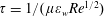$\unicode[STIX]{x1D70F}=1/(\unicode[STIX]{x1D707}\unicode[STIX]{x1D700}_{w}Re^{1/2})$ . However, the general structure and analysis of what we have seen in this paper would remain the same.

The small density ratio, $\unicode[STIX]{x1D70C}$ , has no major effect on our analysis, other than to diminish the role of surface tension in the inner region. The pressure terms in the inner region are $O(\unicode[STIX]{x1D70C})$ , compared to the viscous term, which is of $O(\unicode[STIX]{x1D70C}/\unicode[STIX]{x1D707})$ . Hence the pressure term, and therefore surface tension, has a lower-order effect on the film flow.

To consider a small thermal conductivity ratio, we can simply expand our derived expressions in asymptotic series as $\unicode[STIX]{x1D706}\rightarrow 0$ under appropriate restrictions on the comparative size of $\unicode[STIX]{x1D706}$ and $\unicode[STIX]{x1D700}_{w}Re^{1/2}$ .

We have also neglected several physical effects in this paper. The exclusion of gravity and viscous dissipation in the two fluids was for a matter of convenience; these effects could readily be brought back into the model. However, perhaps the boldest assumption made in the derivation was that the flow parameters are independent of the fluid temperature. In aircraft icing conditions, the external air flow is typically subzero. The plate temperature, which plays the role of an anti-icing heating element, is typically very high, since these elements often make use of the bleed heat from the aircraft engines. Therefore, due to this large range of temperatures, we might expect there to be significant variation in the fluid properties. These considerations will form part of future work.

6.2 Summary

In this paper, we have modelled the freezing of a thin film situated within an aerodynamic boundary layer due to the loss of heating on part of a flat plate. Throughout, we have assumed that the liquid film is much thinner than the air boundary layer thickness. We systematically derived models for the behaviour of the flow before and after freezing.

Prior to freezing, the flow is steady, as described by the work of Nelson et al. (Reference Nelson, Alving and Joseph1995) and Timoshin (Reference Timoshin1997). The thermal problem is driven by the changing plate boundary condition. We looked at a specific case where the plate temperature cools sufficiently slowly that the thermal problem is quasi-steady, with time only entering through the boundary condition. Due to the change in film temperature, a sublayer develops in the air thermal boundary layer in which the temperature changes from the steady profile to the reduced film temperature. We used the Lighthill approximation on the flow variables to solve for the temperature in this sublayer analytically.

Once the plate temperature reaches the freezing temperature at time $t=t_{c}$ , ice begins to form on the plate. We assumed throughout that the ice growth rate has a leading-order effect on the film velocity profile. We outlined two temporal regimes. When $t-t_{c}=O(1)$ , the ice layer is thin and the temperature jump across the ice is small. Since the ice is so thin, the film thickness only changes by a small amount from its steady solution. In the second temporal regime, when $t-t_{c}=O(1/(\unicode[STIX]{x1D700}_{w}Re^{1/2}))$ , the ice layer is comparable to the film in thickness, which causes a leading-order variation to the steady-state solution.

When $t-t_{c}=O(1)$ , there are three distinct asymptotic regions: an outer region where the length and velocity scales are the same as the steady-state problem; an inner region close to the switch-off point where the air and film heat fluxes balance on the free surface; and an intermediate region in which the free surface profile can be matched between the inner and outer solutions.

Upstream of the switch-off point, the outer flow is unchanged from the steady solution. In the outer region downstream of the switch-off point, since the film is much thinner than the air boundary layer, ice growth is driven purely by the heat flux from the ice layer. Hence, the height of the ice layer depends purely on the applied temperature on the plate: if the applied temperature is uniform along the plate, ice growth is uniform along the plate. Therefore, the outer region sees the ice layer as a small step on the plate. In the regime in which the film is thinner than the classical lower-deck scale, this step is not enough to trigger viscous–inviscid interaction at leading order. In the inner region, the flow solution is simply given by the local shear profile of the boundary layer solution, while the thermal problem is straightforward to solve numerically. For our specific plate temperature profile, we showed that the ice growth rate in the inner region is proportional to $t-t_{c}$ , with an $x$ -dependence coming through the film heat flux evaluated on the ice surface.

The inner and outer solutions for the film thickness are matched via an intermediate region in which there is a full balance in the kinematic equation. The free surface is continuous, but not smooth, with a slope discontinuity propagating along the characteristic that emanates from the switch-off point at $t=t_{c}$ . Upstream of the slope discontinuity, the free surface profile is driven by the steady-state flux, while downstream the free surface is driven by the mass loss due to freezing.

When 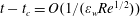$t-t_{c}=O(1/(\unicode[STIX]{x1D700}_{w}Re^{1/2}))$ , the characteristic along which this slope discontinuity propagates enters the outer region. Furthermore, on this time scale, the ice thickness is of the same order of magnitude as the film. We now must solve a nonlinear hyperbolic equation in the outer region for the film thickness. Matching with the small-time solution gives an initial profile that is continuous but not smooth. The slope discontinuity in the free surface is accentuated by the nonlinearity and eventually leads to shock formation. We solved the equation numerically and showed that the film can rupture in finite time. The location and speed of rupture depend strongly on the size of the applied temperature at the wall.

Naturally, since the film thins rapidly before rupture, our assumption that its thickness is of the same order of magnitude as the ice breaks down. While we have not looked in detail at what happens when this assumption breaks down, it is interesting to postulate on possible behaviours. There is a large bulk of liquid upstream of the touchdown, while downstream the film is much thinner, and is freezing rapidly. It seems likely that a bias toward ice growth will form upstream of film rupture, causing an ice hump to develop close to the switch-off point. This is akin to the ice ‘horns’ seen in runback flow on aircraft. In conditions when the surrounding air has a high liquid water content and is close to the freezing temperature, not all of the film freezes on the aircraft elements. Some water flows aft along the elements, with a localised thickening of the ice layer forming ‘horned’ or ‘beaked’ ice shapes. Whether or not we see this in our model after rupture remains to be studied.