


1. Introduction
Precession corresponds to the continuous rotation of the direction of the spin axis of any rotating body, e.g. a spinning top. It has been widely studied in fluid mechanics, not only because of the large range of possible applications in industrial and natural flows (see e.g. Vanyo Reference Vanyo1993), but also because of its appeal from a fundamental point of view: there is indeed a striking contrast between the apparent simplicity of the precession forcing and the complexity of the excited flows. Even at weak forcing amplitude, various types of boundary and bulk instabilities, as well as waves, zonal flows and turbulence, are excited in all investigated geometries, including the cylinder (e.g. Gans Reference Gans1970; Meunier et al. Reference Meunier, Eloy, Lagrange and Nadal2008; Herault et al. Reference Herault, Gundrum, Giesecke and Stefani2015), the cube (e.g. Goepfert & Tilgner Reference Goepfert and Tilgner2016), the sphere (e.g. Kida Reference Kida2011; Boisson et al. Reference Boisson, Cébron, Moisy and Cortet2012; Goto et al. Reference Goto, Matsunaga, Fujiwara, Nishioka, Kida, Yamato and Tsuda2014; Lin, Marti & Noir Reference Lin, Marti and Noir2015), the spherical shell (e.g. Triana, Zimmerman & Lathrop Reference Triana, Zimmerman and Lathrop2012; Cébron et al. Reference Cébron, Laguerre, Noir and Schaeffer2019), the spheroid (e.g. Kerswell Reference Kerswell1993; Horimoto, Katayama & Goto Reference Horimoto, Katayama and Goto2020; Kida Reference Kida2020) and the ellipsoid (e.g. Cébron, Le Bars & Meunier Reference Cébron, Le Bars and Meunier2010; Noir & Cébron Reference Noir and Cébron2013). Numerous open questions remain regarding the flow forced by precession, and in particular we still lack experimental confirmation of the various theoretically suggested processes for instability (see e.g. Le Bars, Cébron & Le Gal Reference Le Bars, Cébron and Le Gal2015).
Here we focus on precession in an oblate spheroid, which has been studied for more than a century (Hough Reference Hough1895; Sloudsky Reference Sloudsky1895) because of its relevance for planetary dynamics, in particular for the Earth's core dynamics and, possibly, its magnetic field generation (e.g. Bullard Reference Bullard1949; Malkus Reference Malkus1968; Vanyo, Wilde & Cardin Reference Vanyo, Wilde and Cardin1995; Lorenzani & Tilgner Reference Lorenzani and Tilgner2001; Noir, Jault & Cardin Reference Noir, Jault and Cardin2001). The analytical solution first given by Sloudsky (Reference Sloudsky1895) and then by Poincaré (Reference Poincaré1910) for an inviscid flow is characterized by a uniform vorticity. The precession, spin and fluid axes are in the same plane, and the inclination of the fluid rotation axis depends on the geometry and on the Poincaré number, defined as the ratio of the precession to spin rate. This so-called Poincaré's solution is, however, not unique due to the lack of boundary conditions. The classical hypothesis then consists in considering that the component of the fluid rotation along the spin axis has the same amplitude as the container rotation. The solution diverges when the Poincaré number reaches a specific negative value related to the container oblateness and precession angle, a mechanism explained by the resonance of the Poincaré's solution with the so-called tilt-over inertial mode of the rotating fluid (Greenspan Reference Greenspan1968). Accounting for the viscosity is necessary for an accurate, regularized solution: this was first done by Busse (Reference Busse1968), who extended Poincaré's work by considering the interaction of the interior solid-body rotation with the Ekman boundary layer, following Stewartson & Roberts (Reference Stewartson and Roberts1963). The three components of the fluid solid-body rotation are then solutions of a system of three nonlinear coupled equations, which was also recovered by Noir et al. (Reference Noir, Cardin, Jault and Masson2003) using a less mathematical approach.
Similarly to Poincaré's solution, Busse's solution exhibits a specific behaviour in the vicinity of its resonance with the tilt-over eigenmode of the rotating fluid. Depending on the value of the Ekman number (i.e. the ratio of viscous to Coriolis forces), three separate solutions for the fluid vorticity vector might be possible at a given resonant Poincaré number: (i) a weakly inclined state, which is the relevant solution at small precession forcing, where the fluid rotation axis is close to the container axis and close to the plane comprising the container and the precession axes; (ii) a strongly inclined state with three vorticity components of similar amplitude, which is relevant for more negative Poincaré numbers; and (iii) an unstable solution in between. Bistability and hysteresis between the two former states are thus expected, as in the latter studied theoretically in full detail by Cébron (Reference Cébron2015). Hysteresis was indeed observed using torque measurements in the seminal experiment by Malkus (Reference Malkus1968), for a precession angle of  $96^{\circ }$ in his notation, corresponding here to a precession angle of
  $84^{\circ }$ with a retrograde precession. In fact, in the limit of a large precession angle (i.e. close to
  $90^{\circ }$), the Busse (Reference Busse1968) solution also predicts a second resonance, this time for prograde precession (i.e. a positive Poincaré number): associated bistability and hysteresis were observed in the recent experiment by Horimoto et al. (Reference Horimoto, Simonet-Davin, Katayama and Goto2018), for a precession angle of
  $90^{\circ }$. But, to the best of our knowledge, hysteresis around the retrograde resonance at moderate precession angle has not been experimentally observed yet, despite careful exploration using ultrasonic Doppler anemometry by Noir et al. (Reference Noir, Cardin, Jault and Masson2003), who otherwise closely recovered Reference BusseBusse's (Reference Busse1968) predictions.
Beyond the constant-vorticity base flow and its dynamics, the route to turbulence for precessing flows in spheroids is still an open question, of fundamental importance for planetary applications (Kerswell Reference Kerswell1996). Many instabilities are possible to trigger turbulence. First, the Ekman boundary layer, which reconnects the inclined rotation of the fluid with the imposed rotation of the container, is subject to a strong shear: it might thus become unstable, as described numerically by Lorenzani & Tilgner (Reference Lorenzani and Tilgner2001, Reference Lorenzani and Tilgner2003). Then, Busse (Reference Busse1968) also showed in his theoretical study that the Ekman layer erupts at critical latitudes and generates in the bulk a vertical, geostrophic, shear layer: this localized and intense jet could also destabilize following a classical shear instability, as suggested in the experimental studies of Malkus (Reference Malkus1968) and Vanyo et al. (Reference Vanyo, Wilde and Cardin1995). Ekman layer eruption also generates an oscillating conical shear layer in the bulk, with an azimuthal wavenumber  $m=1$: this periodic forcing can excite a parametric resonance with two inertial waves of the rotating fluid, as carefully demonstrated in the sphere by Lin et al. (Reference Lin, Marti and Noir2015) and in good agreement with the experimental results of Goto, Fujiwara & Yamato (Reference Goto, Fujiwara and Yamato2011) (but see also Kida Reference Kida2019). This mechanism, called a conical shear instability (CSI), has recently been confirmed experimentally in a precessing spheroid by Horimoto et al. (Reference Horimoto, Katayama and Goto2020). Finally, matching the inclined Busse's constant-vorticity solution with the spheroidal boundary of the container induces two corrections to the otherwise circular streamlines (Kerswell Reference Kerswell1993): an elliptical distortion with azimuthal wavenumber
  $m=2$, and a shear due to their misaligned centres with azimuthal wavenumber
  $m=1$. As described analytically by Kerswell (Reference Kerswell1993) and later extended by Wu & Roberts (Reference Wu and Roberts2011), both corrections are also capable of sustaining a parametric instability, which has nevertheless never been convincingly observed in a spheroid, except in numerical simulations with ad hoc boundary conditions to prevent other types of instability (Lorenzani & Tilgner Reference Lorenzani and Tilgner2003; Wu & Roberts Reference Wu and Roberts2009).
The goal of this paper is to provide a better understanding of the base flow and instabilities excited inside an oblate spheroid in precession near the resonance with the tilt-over mode, using laboratory experiments. The material and methods are described in § 2. Then § 3 provides an experimental validation of the hysteretic cycle between two (Busse Reference Busse1968) solutions, as theoretically described by Cébron (Reference Cébron2015). In § 4, we investigate the bulk destabilization of those two solutions, trying to decipher between the various theoretical models for the origin of the involved instability (Kerswell Reference Kerswell1993; Lin et al. Reference Lin, Marti and Noir2015). Finally, § 5 gives a short overview of our results as well as some possible targets for future experimental investigations.
2. Material and methods
2.1. Experimental set-up
In this paper, we study the flow of an incompressible fluid inside an ellipsoid of revolution (or spheroid) in precession. The experimental set-up is described in figure 1. A spheroid of equatorial semi-major axis  $A= 8.5$ cm and axial semi-minor axis
  $B= 7.2$ cm rotates at the angular velocity
  $\varOmega _{0}$ around its axis and is mounted on a platform which rotates at the angular velocity
  $\varOmega _{1}$. The oblateness of the spheroid
  $\eta$, defined by
  $\eta =1-B/A$, is equal to 0.15. The oblateness is constant in our whole study. The spheroid is filled with water with a kinematic viscosity
  $\nu$ known within 2 % from its temperature measurement. The spheroid is carved inside a cylinder in order to minimize the optical deformations when viewing along the cylinder's axis. The angular velocities of the spheroid and of the rotating platform can be varied independently. The angular velocity
  $\varOmega _{0}$ can vary between
  $0.25$ and
  $48$ rad s
 $^{-1}$ and is measured with an accuracy of
  $0.1\,\%$. The angular velocity of the platform
  $\varOmega _{1}$ can be varied from
  $0.01$ to
  $6$ rad s
 $^{-1}$ with increments of
  $0.01$ rad s
 $^{-1}$ and is measured with an accuracy of
  $0.2\,\%$. The cylinder axis is tilted relative to the axis of the platform with an angle
  $\theta$, which can be increased up to
  $30^{\circ }$ and which is determined with an absolute accuracy of
  ${\pm }0.5^{\circ }$. The inclination angle
  $\theta$ can be modified while the platform is rotating thanks to a small motor mounted on the platform and controlled externally. It should be noted that the spheroid is off-centred with respect to the axis of the platform, which does not influence the flow in the absence of free surface and density variations. Indeed, it simply adds a centrifugal force, which is automatically compensated by a pressure gradient.

Figure 1. Sketch of the experimental set-up. A spheroid of equatorial radius  $A$ and minor axis
  $B$ is filled with water and put inside a cylinder which rotates at the angular velocity
  $\varOmega _0$ around its axis
  ${\hat {\boldsymbol z}}$. The spheroid is laying on a turntable and is tilted with an angle
  $\theta$ with respect to the axis
  ${\boldsymbol k}_p$ of the platform. The turntable rotates at an angular velocity
  $\varOmega _1$ along
  ${\boldsymbol k}_p$, which is vertical here. A laser and cameras also lay on the turntable for PIV measurement or mica particle observations.
Two types of measurements are performed. The first one is qualitative and consists of seeding the flow with flat reflective particles, which are known to preferentially align with the local shear. Mica particles of average diameter of  $50\ \mathrm {\mu }$m covered with a titanium dioxide layer to improve reflections are used. A laser diode is used to illuminate a meridian plane of the spheroid and a camera is used to record images at
  $25$ frames per second. The second type of measurement is particle image velocimetry (PIV), which is performed by seeding the flow with passive particles of diameter
  $40\ \mathrm {\mu }$m and density
  $0.996$. The particles are illuminated with a thin light sheet created by two 170 mJ yttrium aluminium garnet pulsed lasers. A cylindrical lens is used to provide this laser sheet. Two small mirrors are also added to redirect the rays in the shadows of the luminous cross-section (due to the refraction of the rays on the cylinder). The laser sheet is fixed relative to the rotating table frame (i.e. the precessing frame) and perpendicular to the axis of the spheroid. The height
  $H$ between the laser sheet and the equatorial plane of the spheroid can be adjusted. The experiments were performed at several fixed heights measured from the equatorial plane between
  $H = 0.2$ and
  $H = 3$ cm. A video camera mounted on the rotating platform and aligned with the axis of the spheroid is used to record the PIV images.
To obtain the velocity field, two successive images are first rotated around the centre of the spheroid to remove the mean solid-body rotation of the flow: this increases the accuracy of the measurements. The images are then treated by a cross-correlation algorithm detailed in Meunier & Leweke (Reference Meunier and Leweke2003). The solid-body rotation is finally added, leading to the transverse velocity field and the axial vorticity. It should be noted that the mean solid-body rotation of the flow is in general smaller than the angular velocity  $\varOmega _0$ of the spheroid. It is unknown before the PIV measurement and it was thus adjusted by trial and error for each experiment. There is a radial cutoff on the images at
  $0.95 R$ (where
  $R$ is the radius of the boundary on the images) beyond which the images are reconstructed by mirror symmetry using
  $I(0.95R+\varepsilon )=I(0.95R-\varepsilon )$. This prevents strong spurious vectors due to the presence of the boundary. The camera and the pulsed lasers are set up so the time
  $\textrm {d} t$ between the two pulses can be adjusted between 1 and 60
  $\mathrm {\mu }$s. The value of
  $\textrm {d} t=0.08/\varOmega _0$ was the optimal choice, since it allowed for a maximal displacement by the flow perturbations, while preventing a too large displacement by the solid-body rotation. The experiments were performed at two different frequencies of acquisition:
  $24$ Hz (i.e. maximal frequency of the camera) and
  $23$ Hz to quantify any stroboscopic effect for the fast modes. For example, let us assume that a peak is measured in the 23 Hz spectrum at the frequency
  $f_{23}$ and at the frequency
  $f_{24}$ in the 24 Hz spectrum. If
  $f_{23}=f_{24}$, it means that there is no stroboscopic effect. But if the two frequencies
  $f_{23}$ and
  $f_{24}$ are different, it means that the true frequency
  $f$ of the peak satisfies
  $f=f_{23}+23 n= f_{24}+24 n'$, with
  $n$ and
  $n'$ integers.
2.2. Theoretical formulation and dimensionless parameters
The flow inside the spheroid is considered incompressible and the kinematic viscosity  $\nu$ of the fluid is assumed constant. The equations of motion are written in the precessing frame, i.e. rotating at
  $\varOmega _1$. However, the axes are tilted so that the
  $\hat {\boldsymbol {z}}$ axis corresponds to the (steady) axis of the spheroid. The Navier–Stokes equations are then
 \begin{gather} \frac{\partial {{\boldsymbol U}}}{\partial t} + {{\boldsymbol U}}\boldsymbol{\cdot}\boldsymbol{\nabla}{{\boldsymbol U}} + 2{\boldsymbol \varOmega}_1\times {{\boldsymbol U}} = -{\boldsymbol \nabla} \varPi + \nu \nabla^{2} {{\boldsymbol U}}, \end{gather}
 \begin{gather}\boldsymbol{\nabla}\boldsymbol{\cdot}{{\boldsymbol U}} = 0, \end{gather}
where  $k_p$ corresponds to the steady unit vector aligned with the platform's axis (see figure 1b). Both PIV measurements and particle visualizations are made in this frame of reference. The centrifugal force is included in a reduced pressure term
  $\varPi =p/\rho +|{\boldsymbol \varOmega }_1 \times {\boldsymbol r}|^{2}/2$, where
  $p$ is the pressure,
  $\rho$ is the constant fluid density and
  $\boldsymbol {r}$ is the vector position. The boundary conditions are no-slip so that the velocity at the boundaries of the spheroid matches that of the spheroid. By taking the semi-major axis
  $A$ as the reference length scale and
  $\varOmega _0^{-1}$ as the reference time scale, the non-dimensionalized equations are
 \begin{gather} \frac{\partial {{\boldsymbol u}}}{\partial t} + {{\boldsymbol u}}\boldsymbol{\cdot}\boldsymbol{\nabla}{{\boldsymbol u}} + 2 P_o \boldsymbol{k}_p \times {{\boldsymbol u}} = -{\boldsymbol \nabla} \varPi + E \nabla^{2} {{\boldsymbol u}}, \end{gather}
 \begin{gather}\boldsymbol{\nabla}\boldsymbol{\cdot}{{\boldsymbol u}} = 0, \end{gather}
where we have introduced the Ekman number  $E=\nu /(\varOmega _0 A^{2})$ and the Poincaré number
  $P_o=\varOmega _1/\varOmega _0$.
Following Busse (Reference Busse1968), the global torque balance for steady solutions is given by
 \begin{equation} 2P_o\int_V \boldsymbol{r} \times (\boldsymbol{k}_p \times \boldsymbol{u}) \text{d}V =-\int_S\varPi\boldsymbol{r}\times\boldsymbol{n}\,\text{d}S +E\int_V\boldsymbol{r}\times\nabla^{2}\boldsymbol{u}\,\text{d}V, \end{equation}
where  $\boldsymbol {r}$ is the vector position,
  $V$ is the volume,
  $S$ is the spheroidal surface and
  $\boldsymbol {n}$ is the surface normal pointing outwards. The precessional torque is balanced by the pressure and viscous torques. In the spherical case, the pressure torque vanishes, which is not true in our spheroidal case. Looking for a uniform vorticity solution to (2.3) of the form
  $\boldsymbol {\varOmega }_F \times \boldsymbol {r}$, Busse (Reference Busse1968) derived an implicit equation for the fluid rotation vector
  $\boldsymbol {\varOmega }_F$ (Busse Reference Busse1968; Noir et al. Reference Noir, Cardin, Jault and Masson2003):
 \begin{equation} \boldsymbol{\varOmega}_F=\frac{X\varOmega_F^{2} P_o}{X^{2}+Y^{2}}\sin\theta\, \hat{\boldsymbol{x}}+\frac{Y\varOmega_F^{2} P_o}{X^{2}+Y^{2}}\sin\theta\, \hat{\boldsymbol{y}}+\varOmega_F^{2} \hat{\boldsymbol{z}}, \end{equation}
with
 \begin{gather} X=0.259\left(\frac{E}{\varOmega_F}\right)^{1/2}+\eta\varOmega_F^{2}+P_o\cos\theta, \end{gather}
 \begin{gather}Y=2.62(E\varOmega_F)^{1/2}, \end{gather}
where  $\varOmega _F=|\boldsymbol {\varOmega }_F|$. Note that this solution is only valid in the limit of small Ekman numbers and small oblateness
  $\eta$.
3. Hysteretic cycle of Busse's solution
For high enough precession angle and oblateness, and small enough Ekman number, the steady flow given by Busse (Reference Busse1968) splits into three different solutions, which have been studied theoretically by Cébron (Reference Cébron2015). The main objective of this section is to address the stability of those solutions, including the bistability and associated hysteretic cycle theoretically described by Cébron (Reference Cébron2015).
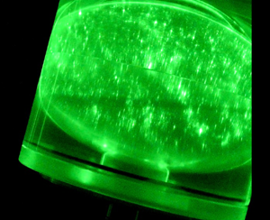
The precession angle is fixed at  $\theta = 15^{\circ }$ while the Poincaré and Ekman numbers are systematically varied. We start by qualitatively observing the mean solid-body rotation with the mica particles method as shown in figure 2 and previously done by Noir et al. (Reference Noir, Cardin, Jault and Masson2003). As shown in figure 2(a) for
  $E=2.3\times 10^{-5}$ and
  $P_o=-8.7\times 10^{-2}$, the axis of rotation of the fluid is tilted towards the direction opposite to the axis
  $\hat {\boldsymbol {x}}$ (see also supplementary movie VisuS1.avi available at https://doi.org/10.1017/jfm.2020.938). When
  $P_o$ is shifted to a value of
  $P_o=-9.1\times 10^{-2}$, as shown in figure 2(b) (and in supplementary movie VisuS1toS2.avi), the flow looks qualitatively different and it is possible to discern an axis of rotation tilted towards
  $+\hat {\boldsymbol {x}}$. Additionally, unsteady small-scale fluctuations are also evidenced by the rapid motion of the mica particles, as shown in the supplementary movies associated with these two figures. When
  $P_o$ is increased back to its initial value, the axis of rotation of the fluid remains tilted towards the
  $+\hat {\boldsymbol {x}}$ direction, until we reach the value
  $P_o=-6.1\times 10^{-2}$ for which the axis of rotation shifts back to an inclination towards
  $-\hat {\boldsymbol {x}}$ (see supplementary movie VisuS2toS1.avi). A transition from two different flows is observed, and for this particular angle of precession of
  $15^{\circ }$, the bistability between the two flows is very clear.

Figure 2. Visualizations of the flow with mica particles in a vertical plane lit with a laser sheet for  $E=2.3\times 10^{-5}$ and
  $\theta =15^{\circ }$: (a)
  $P_o=-8.7\times 10^{-2}$ (see also supplementary movie VisuS1.avi) and (b)
  $P_o=-9.1\times 10^{-2}$ (see also supplementary movie VisuS1toS2.avi for the transition between the two regimes). The position of the PIV plane along the
  $z$ axis is shown by the dashed line. The qualitative direction
  $\boldsymbol {\varOmega }_F$ around which the fluid rotates is shown by the red arrow.
To quantify the bistability better, we now rely on PIV measurements in a narrow region of parameters. As in previous studies (Poincaré Reference Poincaré1910; Busse Reference Busse1968; Noir et al. Reference Noir, Cardin, Jault and Masson2003; Cébron Reference Cébron2015), we assume that the flow essentially consists of a solid-body rotation around an axis  $\boldsymbol {\varOmega }_F=(\varOmega _x,\varOmega _y,\varOmega _z)$, whose components we would like to measure experimentally. The PIV measurements are made in a plane located at a dimensionless distance
  $h=H/A=0.28$ above the equatorial plane of the spheroid. An example of such measurement is shown in figure 3(a) where one can observe the velocity vector field in the PIV plane. The azimuthal velocity along a diameter (passing through the centre of the solid-body rotation) is also plotted in figure 3(b). Despite some weak variations, the measured velocity profile is very close to linear, confirming the solid-body nature of the rotation in the first regime.

Figure 3. (a) Velocity field obtained by PIV in the plane  $z=h=H/A=0.28$ for the first regime, at
  $E=2.3\times 10^{-5}$,
  $P_o=-8.7\times 10^{-2}$ and
  $\theta =15^{\circ }$. Only a quarter of the total number of vectors are plotted for clarity. (b) Symbols show the azimuthal velocity along the red segment plotted in panel (a), with
  $r$ the coordinate along the red axis oriented towards increasing
  $x$ and with
  $r=0$ corresponding to the spheroid axis. (c) Azimuthal velocity profile for the second regime at
  $E=2.3\times 10^{-5}$,
  $P_o=-8.9\times 10^{-2}$ and
  $\theta =15^{\circ }$. In panels (b,c), the solid line corresponds to the theoretical velocity profile for a solid-body rotation fitted from the experimental velocities.
Figure 3(c) shows the azimuthal velocity in the second regime. It remains very close to a linear profile, with fluctuations smaller than 10 % of the velocity of the spheroid. It indicates that the flow is again very close to a solid-body rotation despite the presence of small-scale structures in the flake visualizations of figure 2(b) and the associated supplementary movie. Note that the centre of rotation is not at the centre of the cross-section because  $\boldsymbol {\varOmega }_F$ is tilted with respect to the
  $\hat {\boldsymbol {z}}$ axis and the measurements are made above the equator. It is possible to fit the experimental two-dimensional velocity field with a three-dimensional solid-body rotation
  $\boldsymbol {\varOmega } _F\times \boldsymbol {r}$, where
  $\boldsymbol {r}$ is the position vector, using a standard least-squares approach. In the plane of measurement
  $z=h$, this leads to
 \begin{equation} \begin{bmatrix} u_x \\ u_y \end{bmatrix}= \begin{bmatrix} -y\varOmega_z+h \varOmega_y \\ x\varOmega_z-h\varOmega_x \end{bmatrix}.\end{equation}
A very good agreement is obtained between the experimental and the fitted azimuthal velocities, as shown in figure 3(b), with an error of the order of a few per cent.
Now that we can accurately measure the average orientation of the fluid rotation, we systematically vary the Poincaré number for a fixed Ekman number  $E=2.3\times 10^{-5}$. The results are shown in figure 4. We first discuss the transition as
  $P_o$ is decreased, shown by the circles in figure 4. The Poincaré number is gradually modified while the experiment is running by adjusting the rate of precession
  $\varOmega _1$. We ensure that each solution has reached a steady state by waiting for at least 600 rotation periods between each modification of the Poincaré number. As
  $P_o$ is decreased to a critical value of
  $P_o=-9.1\times 10^{-2}$, the solid-body rotation suddenly shifts to another solution. The first solution (S1 in the following) is the closest to a solid-body rotation aligned with the spheroid:
  $\varOmega _z$ is between
  $0.9$ and
  $1$ while
  $\varOmega _x$ and
  $\varOmega _y$ are much smaller. When the second solution (S2 in the following) is reached, all three components of the rotation vector change significantly. When
  $P_o$ is increased back to its initial value (cross symbols in figure 4), the solid-body rotation remains on S2 past the critical value
  $P_o=-9.1\times 10^{-2}$ and finally shifts back to S1 for
  $P_o=-6.3\times 10^{-2}$. A hysteresis cycle is formed. The transition between S1 and S2 is subcritical.

Figure 4. Components of the rotation rate  $\boldsymbol {\varOmega }_F$ as a function of the Poincaré number for
  $E=2.3\times 10^{-5}$,
  $\theta =15^{\circ }$ and
  $h=H/A=0.33$. These experiments correspond to a gradual decrease (symbols
  $\circ$) and to an incremental increase (symbols
  $+$) of the Poincaré number. The continuous lines correspond to the three Busse's solutions obtained numerically. The dashed lines show the Busse's solutions for S2 when accounting for a turbulent boundary layer with a torque given by (3.2) rather than (2.4c). The arrows indicate the transitions between solutions.
The observed bistability is correctly described by the viscous Busse's solution, implicitly given by (2.4). This equation is solved numerically and results are plotted in figure 4 along with the experimental measurements. Busse's theory plotted in figure 4 in solid lines predicts the hysteretic cycle and is qualitatively consistent with the experimental results. The solution S1 is in red, the solution S2 in blue, while a third solution, not observed experimentally, is shown in green. The comparison with the experiments shows a good agreement in the amplitude of the solution S1. For the amplitude of S2, the agreement is not as clear, in particular for  $\varOmega _y$. The critical
  $P_o$ is in good agreement for the
  $\textrm {S}1\rightarrow \textrm {S}2$ transition but the
  $\textrm {S}2\rightarrow \textrm {S}1$ transition occurs earlier in the experiments.
A first possible explanation for the departure from Busse's theory is that the boundary layer is turbulent for S2 at this Reynolds number  $Re=|{\hat {\boldsymbol z}}-{\boldsymbol \varOmega }_F|/\sqrt {E} \sim 150$. Indeed, Sous, Sommeria & Boyer (Reference Sous, Sommeria and Boyer2013) observed that the boundary layer becomes turbulent at
  $Re=150$, which leads to a higher torque on the bulk flow. Following Cébron et al. (Reference Cébron, Laguerre, Noir and Schaeffer2019), one can estimate the torque created by a turbulent boundary layer as
 \begin{equation} Y=\lambda_t |{\hat{\boldsymbol z}}-{\boldsymbol \varOmega}_F|^{2} = \frac{45 {\rm \pi}}{32} \frac{1+ \eta^{5}}{1-\eta^{5}} {u_0}^{2} \sqrt{1-\frac{C_2^{2} u_0^{2}}{k^{2} |{\hat{\boldsymbol z}}-{\boldsymbol \varOmega}_F|^{2}}}, \end{equation}
where  $u_0$ is the solution of
 \begin{equation} \frac{u_0^{2}}{|{\hat{\boldsymbol z}}-{\boldsymbol \varOmega}_F|^{2}}=\frac{k^{2}}{[\log(u_0^{2}/(0.22E))-C_1]^{2}+C_2} \end{equation}
with  $k=0.4$ the Kolmogorov constant and
  $(C_1,C_2)=(3.3,3)$ empirical constants given by Sous et al. (Reference Sous, Sommeria and Boyer2013) for a plane boundary layer. In our case, for
  $E=2.3 \times 10^{-5}$,
  $|{\hat {\boldsymbol z}}-{\boldsymbol \varOmega }_F|$ is always close to 0.75 for the second Busse's solution such that the torque created by a turbulent boundary layer is always close to 0.0162. Replacing the laminar viscous torque
  $Y=-2.62 \sqrt {\varOmega _f E} \sim 0.0109$ by this turbulent torque in Busse's equation (2.4) leads to a new prediction for the solution S2, which is plotted as a blue dashed line in figure 4. This turbulent torque actually corresponds to a turbulent viscosity 2.2 times larger than the molecular value. The experimental results are located between the two theories, which suggests that the boundary layer is not completely turbulent at this Reynolds number
  ${Re\sim 150}$, which corresponds to the transition from a laminar to a turbulent boundary layer (Sous et al. Reference Sous, Sommeria and Boyer2013). In our experiment, the boundary layer has not been analysed, such that it is hard to tell whether it is turbulent or laminar.
Other explanations for this discrepancy could be invoked. First, (3.58) of Zhang, Chan & Liao (Reference Zhang, Chan and Liao2014) suggests that the numerical coefficient 2.62 for  $Y$ in (2.4c) might decrease by 20 % for our spheroid compared with a sphere. Second, (3.57) of Zhang et al. (Reference Zhang, Chan and Liao2014) suggests that the numerical coefficient 0.259 for
  $X$ in (2.4b) might be three times smaller for our spheroid compared with a sphere. However, the induced modifications on
  $X$ and
  $Y$ are too small to explain the discrepancy between the laminar Busse's solution and the experiment. Third, as shown by Kida (Reference Kida2018), the critical latitude moves when the precession rate increases. For precession rates much larger than the rotation rate, the eruption of the boundary layer takes place in a ring at the equator of the precession axis. This might modify the structure of the instabilities. However, these singularities have always been neglected in the calculation of the torque from the boundary to the bulk flow. This modification may not play an important role for the base flow. Finally, the visualizations of figure 2(b) and the corresponding supplementary movie indicate that the bulk flow seems to be more complex than a simple solid-body rotation, with small-scale unsteady structures. We will show in the next section that these are inertial modes which may generate an axisymmetric flow by nonlinear streaming, as is well known for a precessing cylinder (Lagrange et al. Reference Lagrange, Meunier, Nadal and Eloy2011). This can modify the mean solid-body rotation and explain the weak discrepancy between Busse's solution and the experimental results.
Finally, we have systematically varied the Ekman number: both mica particle experiments and PIV measurements are gathered in figure 5. The domain where S1 and S2 can be observed corresponds to the region with black and green symbols. The hysteresis cycle is only observed for Ekman numbers smaller than  $2\times 10^{-4}$. The bistable region increases in size when
  $E$ decreases, as predicted theoretically. However, it is a bit smaller than the theoretical region predicted by Busse: as already seen before, for all explored values of Ekman number, the transition from S2 to S1 occurs for smaller values of the Poincaré number in the experiments, since the solution S2 is unsteady.

Figure 5. Stability diagram of all the experiments as a function of  $E$ and
  $P_o$. Crosses correspond to S1 while circles correspond to S2. The hysteresis region corresponds to black and green symbols. This region is compared with Busse's theory solved numerically using the molecular viscosity, and shown by solid lines. For S1, red and black crosses correspond to steady flows, whereas green crosses correspond to unsteady flows. For S2, blue and black circles correspond to unsteady flows, whereas cyan circles correspond to steady flows.
In conclusion, we have measured the base flow driven by precession in a spheroidal cavity, which can be reasonably approximated by a solid-body rotation as assumed by Busse (Reference Busse1968) in the explored parameter range. A hysteresis cycle is observed for a certain range of Poincaré numbers. This bistable regime, obtained here for a tilt angle of  $15^{\circ }$, is similar to what has been obtained for a larger tilt angle of
  $90^{\circ }$ by Malkus (Reference Malkus1968) and Horimoto et al. (Reference Horimoto, Simonet-Davin, Katayama and Goto2018). A good agreement with Busse's theory is obtained when the flow is stationary, which is the case for solution S1 over almost all the parameter space explored. However, the second solution S2 is slightly different from the prediction by Busse, mainly because this solution does not appear to be stationary in the range accessible to our set-up due to the presence of instabilities. It is therefore natural to study now the hydrodynamic stability of these two solutions, which is the main objective of the following section.
4. Instabilities of the base flow
When the Ekman number is sufficiently low, both Busse's solutions can destabilize via hydrodynamic instability, leading to a turbulent flow far from the threshold. Two different instabilities have been observed depending on the Poincaré and Ekman numbers. They are described in the following close to their threshold.
4.1. Instability of the first Busse's solution
The first Busse's solution S1 can destabilize when the Ekman number is smaller than about  $10^{-5}$ and when the Poincaré number decreases beyond about
  $-$0.07. It corresponds to the green crosses in the stability diagram of figure 5. In this regime, the mean flow remains close to the first Busse's solution and does not switch to the second Busse's solution. However, a perturbation arises with a well-defined frequency
  $f_I$, as shown in the temporal spectrum of figure 6(a). This spectrum is computed from the spectral density of the vorticity, which is averaged over the entire PIV section:
 \begin{equation} E_f = \frac{1}{\rm \pi} \iint_{r<1} |\tilde{\omega}({{\boldsymbol r}},f)|^{2} \, \textrm{d}{{\boldsymbol r}}, \end{equation}
where the temporal Fourier transform of the vorticity is defined as
 \begin{equation} \tilde{\omega}({{\boldsymbol r}},f) = \frac{1}{t_f-t_i} \int_{t_i}^{t_f} \omega({{\boldsymbol r}},t) \exp({\mbox{i} 2 {\rm \pi}f t})\, \textrm{d} t. \end{equation}
It was found that this quantity reveals the instability better than the spectral density of the velocity. This is probably because Busse's solution contains a uniform vorticity which is insensitive to small displacements and because the instability contains small structures which have a large vorticity even for small velocities.

Figure 6. (a) Temporal spectrum and (b) temporal evolution of the spectral density of vorticity defined by (4.1) and measured by PIV at  $h=0.065$. The Poincaré number is decreased at
  $t=0$ from
  $-$0.0826 to
  $-$0.0838. In panel (b), the spectral density is measured at the frequency of the instability
  $f_I$ (in red) and at the frequency of the harmonic
  $f_H$ (in blue); and the duration of the sliding window
  $t_f-t_i$ is equal to 14.3 rotation periods in order to be small compared with the growth time of the instability and large compared with the period of the instability (equal to 0.125 rotation period).
In figure 6(a), the Fourier transform is computed over the total duration of the PIV measurement, i.e. about 350 rotation periods. It leads to an accurate determination of the frequency of the instability  $2 {\rm \pi}f_I = 7.99$. However, it is also possible to measure the Fourier transform over smaller time intervals in order to plot the spectral density as a function of time. For example, figure 6(b) shows the temporal variation of
  $E_{f_I}$ at the frequency
  $f_I$ of the instability. In this experiment, the Poincaré number has been decreased at
  $t=0$ by 1.5 % in order to switch from a stable to an unstable regime. The spectral density of vorticity
  $E_{f_I}$ remains constant during about 300 rotation periods, because the signal is smaller than the noise in the measurement. It then grows by two orders of magnitude until 600 rotation periods where it seems to saturate. This is a clear indication that the flow has become unstable when the Poincaré number has decreased from
  $-0.0826$ to
  $-0.0838$. The growth rate
  $\sigma$ can be estimated by fitting the spectral density with an exponential function
  $\mbox {e}^{2 \sigma t}$ between
  $t/2{\rm \pi} =430$ and 550, leading to
 \begin{equation} \sigma=1.3 \times 10^{-3} \pm 30\,\% . \end{equation}
 It can be noted that the spectrum of figure 6(a) exhibits a small peak at the frequency  $2 {\rm \pi}f_H=0.77$. It has been checked experimentally (by doing the same experiment using two different acquisition frequencies
  $f_{{acqu}}$) that this frequency is shifted by
  $2 {\rm \pi}f_{{acqu}}=16.67$ because the acquisition frequency of the camera is too low. The real frequency of this peak is in fact equal to
  $2 {\rm \pi}f_H= -15.9$, which corresponds to the harmonic of the instability. The spectral density at this frequency
  $f_H$ is plotted in figure 6(b) as a function of time. It starts to increase above the noise level after 500 rotation periods and then grows slightly faster than the primary mode, with a growth rate of the order of
  $\sigma =1.7 \times 10^{-3} \pm 30\,\%$.
Figure 7 shows the spatial structure of the vorticity filtered at the frequency  $f_I$ of the instability. The snapshot is taken towards the end of the exponentially growing regime of the instability in order to get the best signal-to-noise ratio. The real part of the vorticity
  $\tilde {\omega }$ exhibits two concentric rings of vortices. The inner ring contains 18 well-defined vortices of alternate sign. The second ring, located close to the boundary, is less organized despite its larger amplitude. This is probably due to the interference with the boundaries, which decreases the accuracy of the PIV.

Figure 7. (a) Real part of the vorticity filtered at the frequency of the instability  $f_I$ as defined by (4.2). The Fourier transform is calculated over 81.6 rotation periods around
  $t/2 {\rm \pi}=510$ (corresponding to the dashed line of figure 6b). (b) Azimuthal spectrum of the vorticity as a function of the radius at
  $t/2 {\rm \pi}=510$. (c) Azimuthal spectrum integrated over
  $r$, as defined by (4.5) after 306 rotations (purple), after 387 rotations (cyan), after 469 rotations (red), after 551 rotations (green) and after 632 rotations (blue). Lines between the symbols are only here to improve the visibility of the curves. Here,
  $P_o=-0.0838$,
  $E=1.3 \times 10^{-5}$ and
  $h=0.065$.
The azimuthal spectrum of the vorticity can be obtained using an azimuthal Fourier transform:
 \begin{equation} \hat{\tilde{\omega}}_m(r,f_I) = \int_{\theta=0}^{\theta=2{\rm \pi}} \tilde{\omega}(r,\theta,f_I) \,\textrm{e}^{\textrm{i} m \theta} \, \textrm{d}\theta. \end{equation}
It is plotted in figure 7(b) for  $r$ varying from 0.2 to 0.8. The two rings of vortices create two lobes around
  $r=0.4$ and
  $r=0.7$ with an azimuthal wavenumber close to
  $m=9$. By integrating this azimuthal spectrum over
  $r$, it is possible to get the total azimuthal spectrum of the vorticity:
 \begin{equation} E_{f_I,m} = \int_{r=0}^{r=1} |\hat{\tilde{\omega}}_m(r,f_I)|^{2} r \, \textrm{d} r. \end{equation}
This spectrum is plotted in figure 7(c) at different times. All the spectra present a maximum spectral density of vorticity at the azimuthal wavenumber  $m=9$. They also exhibit a moderate vorticity (about 50 % of the maximum) at the azimuthal wavenumber
  $m=8$ and a weak peak (about 20 % of the maximum) at
  $m=6$. This multi-modal signature clearly points towards a parametric instability involving a given forcing and two inertial modes of our rotating fluid.
In fact, this structure with large azimuthal wavenumbers is very similar to the structure that has been observed in a precessing sphere. Lin et al. (Reference Lin, Marti and Noir2015) argued that it was induced by a parametric resonance between the conical shear layer generated at the critical latitude with an azimuthal wavenumber  $m=1$, and two free inertial modes of the sphere with azimuthal wavenumbers
  $m=17$ and
  $m=18$. It is thus tempting to relate the instability observed here with
  $m=9$ and
  $m=8$ to such a CSI. However, the presence of a weak peak at
  $m=6$ indicates that a weak elliptic coupling
  $m=2$ might also be present, which could transfer some energy from
  $m=8$ to
  $m=6$. This coupling could be due to an elliptic instability as described by Kerswell (Reference Kerswell1993). Furthermore, the presence of the two azimuthal wavenumbers
  $m=8$ and
  $m=9$ could also be due to a shear instability described by Kerswell (Reference Kerswell1993), where two free inertial modes are coupled by the mean shear of the flow with
  $m=1$. Note that the latter two instabilities cannot be found in a sphere because they rely on the oblateness of the container.
To try to disentangle the various possible origins of the observed instability, it is useful to determine its inviscid growth rate, which we do by measuring the variation of the viscous growth rate with respect to the Poincaré number. We thus measure the growth rate accurately (within 20 %) by fitting the growth of the amplitude of modes  $m=8$ and
  $m=9$ (rather than the growth of the total spectral density of vorticity) for two different Poincaré numbers. The growth rate increases from
  $1.5 \times 10^{-3}$ to
  $7.3 \times 10^{-3}$ when the Poincaré number decreases from
  $-0.0838$ to
  $-0.0861$, which leads to
 \begin{equation} \frac{\partial \sigma_{{inv}}}{\partial P_o} = - 2.5 \pm 30\,\%. \end{equation}
The measured variation corresponds to the variation of the inviscid growth rate because the viscous damping of the instability is independent of the Poincaré number: it only depends on the Ekman number.
Experimentally, it is also found that the tilt angle  $\theta _f$ of the solid-body rotation defined by
 \begin{equation} \tan \theta_f=\frac{\sqrt{\varOmega_x^{2}+\varOmega_y^{2}}}{\varOmega_z} \end{equation}
varies as
 \begin{equation} \frac{\partial \theta_f}{\partial P_o} = -17 \pm 20\,\% \end{equation}
for these Poincaré and Ekman numbers. Assuming that the inviscid growth rate is proportional to the tilt angle  $\theta _f$ (which is a fair assumption since the inviscid growth rate is proportional to the differential rotation for small tilt angles) gives an empirical formula for the inviscid growth rate
  $\sigma _{{inv}} = 0.15\theta _f \pm 50\,\%$. This equation can also be written
  $\sigma _{{inv}} = 1.4 E^{1/5} \theta _f \pm 50\,\%$ if we assume that the inviscid growth rate scales as
  $E^{1/5}$ as in the CSI (Lin et al. Reference Lin, Marti and Noir2015). Finally, assuming that the viscous damping effect scales as
  $\sqrt {E}$ leads to an empirical formula for the total growth rate if it was due to the CSI (by imposing
  $\sigma =0$ at the threshold where
  $\theta _f=0.32$):
 \begin{equation} \sigma = 1.4 ( E^{1/5} \theta_f - 9.3 \sqrt{E} ). \end{equation}
 For a sphere, it was found experimentally (Goto et al. Reference Goto, Fujiwara and Yamato2011) and numerically (Lin et al. Reference Lin, Marti and Noir2015) that the CSI is unstable if  $|P_o \sin \alpha | - 25.1 E^{4/5}$ is positive. It is thus logical to assume that the growth rate of the CSI is proportional to this term, which can be written as
 \begin{equation} \sigma_{CSI} = C ( E^{1/2} \theta_f/0.3797 - 25.1 E^{4/5}), \end{equation}
since, for a sphere, the tilt angle  $\theta _f$ is given from Busse's solution (see (4.25) and (4.26) in Kida (Reference Kida2013)) by
  $\theta _f \sqrt {E}=0.3797 P_o \sin \alpha$. Multiplying this formula by
  $0.3797 E^{-3/10}$ leads to
 \begin{equation} \sigma_{CSI} = C' (E^{1/5} \ \theta_f - 9.53 \sqrt{E}), \end{equation}
with  $C'=0.3797C E^{-3/10}$. This prediction deduced from the sphere is in excellent agreement with the empirical, experimental formula (4.9) found in this paper for a spheroid. Note that the second term of those equations corresponds to the viscous damping: the value
  $1.4\times 9.3 \simeq 13$ is reasonable compared with other viscous damping prefactors determined for similar resonant instabilities, where it ranges from 2.62 for the spin-over mode to 20 for more complex modes (Grannan et al. Reference Grannan, Le Bars, Cébron and Aurnou2014; Lemasquerier et al. Reference Lemasquerier, Grannan, Vidal, Cébron, Favier, Le Bars and Aurnou2017). The CSI is thus an excellent candidate to explain the observed instability.
In order to compare the experimental growth rate to the predictions of the elliptic instability and the shear instability, it is necessary to calculate the ellipticity and the shear of the base flow. Following Kerswell (Reference Kerswell1993), the velocity is written using new coordinates  $(x',y',z')$ where the
  $z'$ axis is aligned with the axis of rotation of the bulk flow:
 \begin{equation} {{\boldsymbol u}}= \varOmega_{z'} [(-y',x',0) + \beta (y',x',0) + \epsilon (0,z',0)]. \end{equation}
For the normal flow to vanish on the spheroidal surface, the shear must be equal to
 \begin{equation} \epsilon = \frac{2 \eta_K \tan(\theta_f)}{2+\eta_K+2\tan^{2}(\theta_f)} \end{equation}
and the ellipticity must be equal to
 \begin{equation} \beta = \frac{2 \eta_K \tan^{2}(\theta_f)}{(2+\eta_K^{2})+(4+2\eta_K)\tan^{2}(\theta_f)} , \end{equation}
where  $\eta _K=\eta (2-\eta )/(1-\eta )^{2}$ is equal to 0.3841 in our experiments.
The variation of the shear can be calculated from (4.13) as  $\partial \epsilon / \partial \theta _f=-0.27$ at threshold (where
  $\theta _f=0.32$). Using (4.6) and (4.8), it leads to the value
  $\partial \sigma _{{inv}}/\partial \epsilon = 0.54 \pm 50\,\%$. Finally, assuming that the growth rate is proportional to the shear
  $\epsilon$ and adding a viscous damping as
  $\sqrt {E}$ (with a coefficient adjusted such that the growth rate vanishes at
  $\theta _f=0.32$, i.e. at
  $\epsilon =0.11$) gives an empirical formula for the growth rate if it is due to the shear instability:
 \begin{equation} \sigma = 0.54 \epsilon - 14.6 \sqrt{E} . \end{equation}
This formula is in fair agreement with the prediction for the shear instability coming from the linear theory of Kerswell (Reference Kerswell1993), valid in the limit of small oblateness: the first coefficient is expected to be below  $0.6$ and the second coefficient is expected to vary from 2.6 for the spin-over mode to 20 for complex modes (Grannan et al. Reference Grannan, Le Bars, Cébron and Aurnou2014; Lemasquerier et al. Reference Lemasquerier, Grannan, Vidal, Cébron, Favier, Le Bars and Aurnou2017).
Finally, the variation of the ellipticity can be calculated from (4.14) as  $\partial \beta / \partial \theta _f = -0.17$ at the threshold (where
  $\theta _f=0.32$). Using (4.6) and (4.8), it leads to the value
  $\partial \sigma _{{inv}}/\partial \beta = 0.87 \pm 50\,\%$. Finally, assuming that the growth rate is proportional to the ellipticity
  $\beta$ and adding a viscous damping as
  $\sqrt {E}$ (with a coefficient adjusted such that the growth rate vanishes at
  $\theta _f=0.32$, i.e. at
  $\beta =0.032$) gives an empirical formula for the growth rate if it is due to the elliptic instability:
 \begin{equation} \sigma = 0.87 \beta - 7.7 \sqrt{E} . \end{equation}
This formula is again in fair agreement with the linear prediction for the elliptic instability derived in the limit of small oblateness: the first coefficient is expected to be below  $1$, depending on the relative rotation of the fluid and of the elliptic distortion (Le Bars et al. Reference Le Bars, Lacaze, Le Dizès, Le Gal and Rieutord2010), and the second coefficient is expected to vary from 2.6 to 20 (Grannan et al. Reference Grannan, Le Bars, Cébron and Aurnou2014).
To conclude, it thus seems that the instability observed experimentally on mode S1 can be explained theoretically by the three instabilities: shear instability, elliptic instability and CSI. It is actually possible that the three instabilities coexist. It can explain not only the high azimuthal wavenumbers of the unstable modes, but also the presence of three azimuthal wavenumbers ( $m=9$, 8 and 6) separated by
  ${\rm \Delta} m=1$ (characteristic of the CSI and the shear instability) and
  ${\rm \Delta} m=2$ (characteristic of the elliptic instability).
4.2. Instability of the second Busse's solution
The second Busse's solution S2 was found to be unstable in most cases. It corresponds to the blue symbols in the stability diagram of figure 5, which cover a large region of the domain for the solution S2. The only experiments that were found stable for the second Busse's solution correspond to the cyan symbols, which are limited to large Ekman numbers (larger than about  $10^{-4}$).
At threshold, the instability is characterized by a temporal growth of the spectral density of vorticity at a frequency equal to  $2 {\rm \pi}f_I = 2.8$. However, the total spectral density of vorticity only increases by a factor 3 between the initial state and the saturated state. This is due to the strong initial noise in the measurement probably related to the strong tilt of the second Busse's solution, and to the early viscous saturation due to the large Ekman number. This does not allow us to measure a growth rate accurately, which will rather be measured on the amplitude of the azimuthal wavenumbers of the instability. It should be noted that a weaker peak of spectral density of vorticity is also measured at
  $2 {\rm \pi}f_H = 5.6$, which corresponds to the harmonic of the instability's frequency.
Figure 8 shows the spatial structure of the vorticity filtered at the frequency  $f_I$ of the instability at the end of the exponentially growing regime. The real part of the vorticity
  $\tilde {\omega }$, plotted in figure 8(a), exhibits a complex spiralling structure containing about four positive and four negative vortices. The azimuthal spectrum, defined by (4.4), is plotted in figure 8(b). It indeed confirms the predominance of the azimuthal wavenumber
  $m=4$ with the presence of two patches extending from
  $r=0.2$ to 0.4 and from
  $r=0.5$ to 0.6. Integrating the azimuthal spectrum over
  $r$ leads to the azimuthal spectrum of total spectral density of vorticity, as plotted in figure 8(c). It indicates that the vorticity is significantly larger for azimuthal wavenumbers
  $m=3$ and
  $m=4$ than for the other azimuthal wavenumbers. The presence of two azimuthal wavenumbers separated by
  ${\rm \Delta} m=1$ is characteristic of the CSI and the shear instability rather than the elliptic instability. However, note that PIV measurements in a plane located above the equator (at
  $z=0.18$) indicate that there is also a peak for
  $m=6$, which is about
  $50\,\%$ of the peak for
  $m=4$.

Figure 8. (a) Real part of the vorticity filtered at the frequency of the instability  $2 {\rm \pi}f_I = 2.8$ as defined by (4.2). The Fourier transform is calculated over 16 rotation periods around
  $t/2 {\rm \pi}=100$, corresponding to the end of the exponentially growing stage. (b) Azimuthal spectrum of the vorticity as a function of the radius at
  $t/2 {\rm \pi}=100$. (c) Azimuthal spectrum integrated over
  $r$, as defined by (4.5) after eight rotations (purple), after 24 rotations (cyan), after 40 rotations (red), after 56 rotations (green), after 72 rotations (blue), after 87 rotations (black), after 103 rotations (yellow), after 119 rotations (purple), after 135 rotations (cyan) and after 151 rotations (red). Here,
  $P_o=-0.157$,
  $E=1.2 \times 10^{-4}$ and
  $h=0.065$.
By fitting the temporal evolution of the amplitude of modes  $m=3$ and
  $m=4$, it is possible to accurately measure the growth rate
  $\sigma$ of the instability. It was found to be equal to 0.0062 for
  $Po=-0.157$ and to 0.02 for
  $Po=-0.147$ with uncertainties of the order of
  $5\,\%$. As before, assuming that the viscous damping is independent of the Poincaré number, the variation of the inviscid growth rate can be deduced as
 \begin{equation} \frac{\partial \sigma_{{inv}}}{\partial Po} = 1.4 \pm 10\,\%. \end{equation}
As in the previous section, using the fact that  $\partial \theta _f/\partial Po= 3.4 \pm 20\,\%$ at the threshold where
  $\theta _f=0.72$ and
  $E=1.2 \times 10^{-4}$ leads to an empirical formula for the growth rate:
 \begin{equation} \sigma = 2.5 ( E^{1/5} \theta_f - 7 \sqrt{E} ). \end{equation}
with a 30 % error on the numerical value 2.5. Here, the viscous damping has been added in order to satisfy  $\sigma =0$ at threshold. This viscous damping (equal to
  $-17.5\sqrt {E}$) seems to be a bit large. Indeed, it is expected to be smaller than in the previous section (where it was equal to 13) since the azimuthal wavenumbers are lower. However, the Ekman number is larger here, such that the volumetric viscous damping may not be negligible. The term
  $-17.5\sqrt {E}$ could thus be rather equal to
  $10\sqrt {E}+680E$, for example, using ad hoc coefficients (see e.g. a detailed discussion in the closely related case of libration in Lemasquerier et al. (Reference Lemasquerier, Grannan, Vidal, Cébron, Favier, Le Bars and Aurnou2017)). It is also possible that the boundary layer is turbulent in this regime, leading to a larger Ekman pumping and thus a larger damping rate of the inertial modes. This empirical formula is in good agreement with the prediction for the CSI, given by (4.11), where the second coefficient is equal to 9.5 rather than 7.
To compare with the theory of the shear instability, the variation of the shear is calculated at  $\theta _f=0.72$ using (4.13), leading to
  $\partial \epsilon / \partial \theta _f = -0.07 \pm 20\,\%$. It gives an empirical formula for the growth rate if it is due to the shear instability:
 \begin{equation} \sigma = 5.8 \epsilon - 90 \sqrt{E}, \end{equation}
with a 30 % error on the numerical value 5.8. It means that the shear instability is probably not unstable for these parameters. Indeed, the theory predicts that the inviscid growth rate is equal to  $0.6 \epsilon$ rather than
  $5.8 \epsilon$ (Kerswell Reference Kerswell1993), and the viscous damping coefficient seems unreasonably large.
Finally, the variation of the ellipticity is calculated at  $\theta _f=0.72$ using (4.14), leading to
  $\partial \beta / \partial \theta _f = -0.15 \pm 20\,\%$. It gives an empirical formula for the growth rate if it is due to the elliptic instability:
 \begin{equation} \sigma = 2.7 \beta - 25 \sqrt{E}, \end{equation}
with a 30 % error on the numerical value 2.7. It means that the elliptic instability is probably not unstable for these parameters. Indeed, the theory predicts an upper bound for the inviscid growth rate equal to  $\beta$ rather than
  $2.7 \beta$ (Le Bars et al. Reference Le Bars, Lacaze, Le Dizès, Le Gal and Rieutord2010).
To conclude, the instability on this branch is probably due to the CSI. The elliptic and the shear instabilities seem to be stable for the second Busse's solution at this tilt angle.
5. Conclusions
In conclusion, our study confirms the presence of hysteresis between two uniform vorticity solutions around the resonance with the tilt-over mode, in good agreement with the analytical, viscous solution of Busse (Reference Busse1968) and the theoretical description of Cébron (Reference Cébron2015). To the best of our knowledge, this is the first experimental validation of hysteresis for a moderate precession angle: our study thus expands the historical work of Malkus (Reference Malkus1968) and the more recent one by Horimoto et al. (Reference Horimoto, Simonet-Davin, Katayama and Goto2018), considering precession close to  $90^{\circ }$. Note that hysteresis has also been observed at this
  $90^{\circ }$ angle in a cylindrical geometry with aspect ratio 1 by Herault et al. (Reference Herault, Gundrum, Giesecke and Stefani2015). In the first solution S1, the fluid rotation axis is only slightly inclined compared with the container rotation axis and the flow remains laminar in most of the explored range of parameters: its amplitude is then quantitatively similar to the Busse (Reference Busse1968) solution. For the second solution S2, the fluid rotation axis is more inclined and small-scale perturbations are almost systematically observed in addition to the global, large-scale, solid-body rotation: a turbulent viscosity has then to be introduced for quantitative agreement with Busse (Reference Busse1968) solution. This turbulent viscosity is satisfyingly predicted by accounting for turbulent dissipation in the Ekman boundary layer, as described by Sous et al. (Reference Sous, Sommeria and Boyer2013).
For each solution, we observe at low enough Ekman number an instability with a well-defined spectral signature in space and time, suggesting a parametric resonance mechanism involving a forcing and two inertial waves of the rotating fluid. Using PIV measurements around the instability threshold, we have tried to decipher between the three possible origins for the forcing described in the literature: the elliptical distortion of the circular streamlines of the inclined Busse's solution in the spheroid, as introduced by Kerswell (Reference Kerswell1993); the associated shearing of their centres, as also described by Kerswell (Reference Kerswell1993); and the conical shear strain generated from critical latitudes by Ekman layer eruption, as recently depicted in the spherical geometry by Lin et al. (Reference Lin, Marti and Noir2015) and in the spheroidal geometry by Horimoto et al. (Reference Horimoto, Katayama and Goto2020). While the latter mechanism seems appropriate for both Busse's solutions, we are not in the position to completely discard the first two suggestions, especially for the first solution S1. In the range of experimentally accessible parameters, all mechanisms have indeed close growth rates and might superimpose: only a systematic and large-range exploration in terms of Ekman number will allow a clear conclusion to be reached, since only the inviscid growth rate of the CSI explicitly depends on the Ekman number. This is, however, experimentally challenging.
To finish, trends for future experimental studies include the exploration of other ranges of Poincaré number, to look for possible parametric instabilities away from the resonance with the tilt-over mode. It will also be very interesting to describe better the nonlinear saturation of the excited instabilities and the shape of the excited turbulence, i.e. geostrophic versus wave turbulence, as recently done in closely related configurations using libration forcing (Le Reun, Favier & Le Bars Reference Le Reun, Favier and Le Bars2019) and direct forcing (Brunet, Gallet & Cortet Reference Brunet, Gallet and Cortet2020). This fundamental question will indeed have a strong influence on, for example, energy dissipation and magnetic field generation, both questions of great interest for planetary applications.
Acknowledgements
This work was supported by the European Research Council under the European Union's Horizon 2020 research and innovation programme through Grant No. 681835-FLUDYCO-ERC-2015-CoG.
Declaration of interests
The authors report no conflict of interest.
Supplementary movies
Supplementary movies are available at https://doi.org/10.1017/jfm.2020.938.


