


1. Introduction
Over the past several years there has been great interest in designing and using synthetic and biological microswimmers for a variety of biotechnological applications including targeted drug delivery (Medina-Sánchez, Xu & Schmidt Reference Medina-Sánchez, Xu and Schmidt2018; Erkoc et al. Reference Erkoc, Yasa, Ceylan, Yasa, Alapan and Sitti2019; Singh et al. Reference Singh, Ansari, Laux and Luch2019; Bunea & Taboryski Reference Bunea and Taboryski2020; Li, Wan & Mao Reference Li, Wan and Mao2020) and biosensing (Lebègue et al. Reference Lebègue, Farre, Jose, Saulnier, Lagarde, Chevalier, Chaix and Jaffrezic-Renault2018; Trantidou et al. Reference Trantidou, Dekker, Polizzi, Ces and Elani2018). In the context of targeted drug delivery, the microswimmer's surface is most commonly functionalized with a bio-particle cargo, and then directed towards areas of interest by using combinations of endogenous stimuli (e.g. chemotaxis (Park et al. Reference Park, Zhuang, Yasa and Sitti2017; Schauer et al. Reference Schauer, Mostaghaci, Colin, Hürtgen, Kraus, Sitti and Sourjik2018)) and external stimuli (e.g. magnetic fields (Felfoul et al. Reference Felfoul2016; Park et al. Reference Park, Zhuang, Yasa and Sitti2017)). A variety of different cargos have been attached to microswimmers including drug-containing nanoliposomes (Felfoul et al. Reference Felfoul2016), polyelectrolyte multilayer microparticles (Park et al. Reference Park, Zhuang, Yasa and Sitti2017), polymethyl methacrylate microparticles (Schauer et al. Reference Schauer, Mostaghaci, Colin, Hürtgen, Kraus, Sitti and Sourjik2018) and double-micelle microemulsions (Singh et al. Reference Singh, Hosseinidoust, Park, Yasa and Sitti2017). The majority of studies show that the effective diffusivity of the cargo is greatly enhanced by the microswimmer's active locomotion, and is in some cases three to four orders of magnitude larger than the particle's purely passive long-time self-diffusivity (Singh et al. Reference Singh, Hosseinidoust, Park, Yasa and Sitti2017).
At the same time there has been an increased interest in the design and usage of vesicle based microsystems which are capable of passively delivering both drugs and other bio-particles to living cells (Marchianò et al. Reference Marchianò, Matos, Serrano-Pertierra, Gutiérrez and Blanco-López2020). Lipid based nanovesicles (e.g. liposomes) are ideal candidates for the encapsulation and delivery of drugs since they are biocompatible with human cells and are known to interact with living cells through endocytosis and membrane merging (Pattni, Chupin & Torchilin Reference Pattni, Chupin and Torchilin2015). Recently, the mRNA-1273 vaccine candidate, developed by Moderna to address the SARS-CoV-2 pandemic, has utilized a lipid based nanovesicle as the main delivery framework for introducing and eliciting an immune response to the SARS-CoV-2 spike glycoprotein (Jackson et al. Reference Jackson2020). Lipid based vesicles also have various distinct advantages over other drug delivery mechanisms since they can protect the encapsulated drug from chemical and biological degradation, and can be loaded with both hydrophilic and lipophilic drugs that are respectively contained within the vesicle's aqueous core or embedded within the vesicle's membrane (Marchianò et al. Reference Marchianò, Matos, Serrano-Pertierra, Gutiérrez and Blanco-López2020).
In this paper we perform a theoretical fluid mechanical analysis of a system which combines the benefits of the vesicle and microswimmer targeted drug delivery systems. The presence of the vesicle provides a protective, biocompatible and flexible framework for drug encapsulation, while the encapsulated microswimmer provides the vesicle with enhanced super-diffusive motion mediated through hydrodynamic interactions between the microswimmer and the vesicle's wall. Our work is largely motivated by the experimental systems presented by Trantidou et al. (Reference Trantidou, Dekker, Polizzi, Ces and Elani2018) and Takatori & Sahu (Reference Takatori and Sahu2020) in which biological microswimmers have been successfully encapsulated inside of engineered giant unilamellar vesicles (GUVs). In related work, Vutukuri et al. (Reference Vutukuri, Hoore, Abaurrea-Velasco, van Buren, Dutto, Auth, Fedosov, Gompper and Vermant2020) have encapsulated self-propelled Janus colloidal particles inside of GUVs. The vesicle that we model is most similar to their high membrane tension GUV. Using a viscous drop instead of a vesicle, Ding et al. (Reference Ding, Qiu, Casadevall i Solvas, Chiu, Nelson and De Mello2016) have developed microfluidic methods to encapsulate synthetic artificial bacterial flagellates (ABFs) and have studied the collective motion of the drop–ABFs system. We are specifically interested in studying the motility of the combined vesicle and microswimmer system, since by controlling the motion of the microswimmer, the hydrodynamically induced motion of the vesicle may in turn be controlled. Additionally, we find motivation in some of Takatori's unpublished research, where vesicles encapsulating swimming magnetotactic bacteria were observed to translate in the direction of an applied external magnetic field. Since these vesicles are passive bodies, these experiments suggest that the vesicle's motion is induced by hydrodynamic interactions between the active encapsulated bacteria and the vesicle's walls. We develop a theoretical hydromechanical model capable of explaining the underlying mechanism by which the vesicle moves, and the effect of microswimmer type on the vesicle's motion.
Although this work is primarily motivated by the aforementioned experimental systems, the theoretical formulation that we present is general in the sense that other abstractions may be applied in place of the squirmer model to allow for modelling of other biologically active particles or systems. In this way, our model has potential to be used for simulating and understanding more complex biological phenomena and processes such as motor protein induced cytoplasmic streaming (Goldstein & van de Meent Reference Goldstein and van de Meent2015) and fluid exchange during syncytium formation via cell–cell fusion (Feliciano, Nixon-Abell & Lippincott-Schwartz Reference Feliciano, Nixon-Abell and Lippincott-Schwartz2018). We rigorously account for multi-body hydrodynamic interactions (HIs) which have been unequivocally demonstrated to be determining factors in controlling microswimmer dynamics (Drescher et al. Reference Drescher, Dunkel, Cisneros, Ganguly and Goldstein2011; Spagnolie & Lauga Reference Spagnolie and Lauga2012), and which are likely to be important in understanding various cellular processes such as macromolecular diffusion (Ando & Skolnick Reference Ando and Skolnick2010) and assembly of the cellular mitotic-spindle (Shelley Reference Shelley2016; Nazockdast et al. Reference Nazockdast, Rahimian, Zorin and Shelley2017). A differentiating factor in this analysis is the inclusion of full HIs and sampling of lubrication physics on close squirmer–container contact.
We model the encapsulated microswimmer using the so-called squirmer model. The squirmer model, originally formulated by Lighthill (Reference Lighthill1952) and Blake (Reference Blake1971), is a popular model for performing theoretical active matter calculations in low Reynolds number flows. The model is an exact solution to the Stokes equations and describes the motion of a microorganism in an unbounded fluid by using a spherical surface deformation field or slip velocity. In an important set of papers, the squirmer model was used to study the HIs between two swimming microorganisms (Ishikawa, Simmonds & Pedley Reference Ishikawa, Simmonds and Pedley2006), and the rheology of both semi-dilute (Ishikawa & Pedley Reference Ishikawa and Pedley2007a,Reference Ishikawa and Pedleyb) and dense suspensions (Ishikawa, Locsei & Pedley Reference Ishikawa, Locsei and Pedley2008) of microorganisms. Ishikawa and Pedley made an important contribution by noticing that the velocity field of a tangential squirmer could be written in a form independent of basis. In this study, we use this representation up to the first two squirming modes  $B^{sq}_{1}$ and
  $B^{sq}_{2}$.
To date, there have only been a few theoretical fluid mechanics studies which have analysed an encapsulated squirmer. The motion of a single spherical squirmer, encapsulated by a viscous drop, was first studied by Reigh & Lauga (Reference Reigh and Lauga2017). In a second closely related paper, Reigh et al. (Reference Reigh, Zhu, Gallaire and Lauga2017) consider the motion of the viscous drop, and present numerical trajectory simulations (based on boundary element simulations) of the squirmer and drop motions. The analytical models presented in both papers are derived as exact solutions to the Stokes equation for the concentric squirmer–drop geometry since the Laplacian in the Stokes equations separates. Both papers also use a more general squirmer model which features a surface velocity boundary condition with both radial and tangential velocity components. With the added radial velocity components, their numerical simulations show that the drop–squirmer system can move in a stable co-swimming state.
Recently, Sprenger et al. (Reference Sprenger2020) also theoretically examined the low Reynolds number locomotion of a microswimmer encapsulated inside of a viscous drop. They derive the image solution for the point force and dipole singularities inside of a spherical drop, both with a clean surface, or loaded with a surfactant. Using these image solutions, they are able to describe the motion of the microswimmer and drop. The image solutions are an important contribution since they can potentially be used to study the dynamics of groups of encapsulated microswimmers in the dilute suspension limit.
In related work, Nganguia et al. (Reference Nganguia, Zhu, Palaniappan and Pak2020) recently studied the locomotion of a squirmer that is encapsulated by a surrounding Brinkman medium. Motivated by exploring the motion of the squirmer in a heterogeneous fluid, the Brinkman medium is used to model a surrounding viscous gel which does not collectively translate with the squirmer. Their analysis presents exact analytical solutions to the Stokes equations for the swimming speed, flow fields and power dissipation of the squirmer. Numerical simulations were not performed. The squirmer's swimming speed is seen to have a local minimum at a critical thickness in the Brinkman medium. In our work, we observe a similar local minimum in the squirmer's speed, which depends on a critical container–squirmer size ratio.
In this paper we study a system with nearly identical geometry; however, our model solves a different fluid mechanics problem where, instead of a drop or Brinkman medium, a rigid leaky container (thin membrane) is used to confine the squirmer. A Brinkman medium, such as the one used in Nganguia et al. (Reference Nganguia, Zhu, Palaniappan and Pak2020), could be used to model a membrane with finite thickness; however, the thin membrane model, proposed in this paper, is designed to be a minimal model that is capable of explaining both squirmer and vesicle motions. Including the viscous term from the Brinkman equation would not only add additional analytical and numerical complexities, but may not significantly alter the results, since at least for small permeabilities, the Darcy term in the Brinkman equation typically dominates the viscous term. Similar to the techniques used by Nganguia et al. (Reference Nganguia, Zhu, Palaniappan and Pak2020), we obtain analytical solutions for the translational motions of the squirmer and container using streamfunctions and eigenfunction expansion methods, which are in contrast to the methods used by Reigh & Lauga (Reference Reigh and Lauga2017) in which Lamb's general axisymmetric solution is directly used. Our model reproduces two solutions that are special limiting cases of the general solution presented in Reigh et al. (Reference Reigh, Zhu, Gallaire and Lauga2017). The first case is when the viscosity ratio,  $\mu _{e}/\mu _{i}$, between the exterior and inner fluids relative to the drop interface becomes infinite. This corresponds to the case where our leaky container becomes impermeable (see § 3.1 or (3.27) in the limit that
  $\{R_{\perp },R_{\parallel }\} \to \{\infty , \infty \}$). The second case is when their viscosity ratio becomes one, in which case we achieve identical results if we impose no resistance to fluid flow tangential to the membrane (
 $R_{\parallel } = 0$) and infinite resistance to fluid flow normal to the membrane (
 $R_{\perp } \to \infty$). Under these conditions we achieve continuity of the tangential component of the total stress across the membrane which is the usual boundary condition used when describing a viscous drop (Leal Reference Leal2007).
In the numerical portion of our work we present a method that is original and significantly different than the methods used in Reigh et al. (Reference Reigh, Zhu, Gallaire and Lauga2017) and the vast majority of low Reynolds number boundary element literature. While we both use boundary element methods to perform squirmer–container trajectory studies, our formulation is based on Fredholm integral equations of the second kind, uses conformal adaptive meshing techniques and employs a more accurate Galerkin discretization procedure. The method in Reigh et al. (Reference Reigh, Zhu, Gallaire and Lauga2017) uses an inherently less accurate collocation method to discretize the integral equations, a non-conformal adaptive meshing technique which introduces hanging T-nodes, and relies on a direct integral formulation involving a Fredholm integral equation of the first kind, which for mobility problems, tends to be ill posed (Kim & Karrila Reference Kim and Karrila2005). In all other related literature, numerical calculations are not performed.
Our paper is organized as follows. We first obtain exact mobility solutions for both the squirmer and container when the squirmer–container geometry is perfectly concentric. The analytical models serve two purposes: to aid in validating the numerical portion of the work, and to provide comparisons with the analytical solutions for the viscous drop and Brinkman medium studies (Reigh et al. Reference Reigh, Zhu, Gallaire and Lauga2017; Nganguia et al. Reference Nganguia, Zhu, Palaniappan and Pak2020). Section 3.1 derives the mobility solutions in the case of a non-porous container, and in doing so recapitulates a reduced version of the results from Reigh & Lauga (Reference Reigh and Lauga2017, § IV), specialized to purely tangential squirmers, but does so in the context of streamfunctions. Next, we derive mobility solutions for the porous–container and squirmer. The porous container is modelled using a generalization of Darcy's law. Fluid flow through the container's surface is driven by the motion of the squirmer, and made proportional to a jump in fluid stress across the container's surface. In § 4, the squirmer–container fluid mechanics problem is reformulated as a coupled set of second kind boundary integral equations. The system of equations is solved using a Galerkin discretization on Compute Unified Device Architecture (CUDA)-enabled graphics processing units (GPUs). Finally, we perform numerical trajectory simulations of the squirmer and container and analyse general mechanisms by which the squirmer and container move. We close the paper with a summary of our work and provide appendices which give further details related to the analytical and numerical portions of the work. Appendix A presents the streamfunction solutions, and appendix B presents the Galerkin discretization procedure and adaptive meshing technique in detail.
2. Problem formulation
The squirmer–container geometry is illustrated in figure 1 in which the fluid domain is partitioned, relative to the container's surface, into interior, porous and exterior regions respectively represented by  $\varOmega _{i}$,
  $\varOmega _{p}$ and
  $\varOmega _{e}$. The container's normal vector points into
  $\varOmega _{e}$, and the normal vector on the squirmer's surface points into
  $\varOmega _{i}$. The interior fluid region,
  $\varOmega _{i}$, is bounded by the squirmer and inner container surfaces,
  $\varGamma _{sq} \cup \varGamma _{c}$. The fluid in all regions is water, with a shear viscosity of
  $\mu = 10^{-3}\ \textrm {Pa}\ \textrm {s}$, and density
  $\rho _{f} = 10^{3}\ \textrm {kg}\ \textrm {m}^{-3}$. For a squirming particle with size
  $a \sim 1\text {--}100 \ \mathrm {\mu }\textrm {m}$ and characteristic velocity
  $U^{sq} \sim 1\text {--}100\ \mathrm {\mu }\textrm {m}\ \textrm {s}^{-1}$, the Reynolds number is
  $Re \sim 10^{-6}\text {--}10^{-2}$, which implies that the squirmer moves at low Reynolds number,
  $Re \ll 1$, and that inertia plays no significant role in the squirmer's propulsion. Under these conditions the fluid mechanics and motion of the squirmer and container are governed by the steady Stokes equations and continuity equation for incompressible flows
 \begin{gather} \mu \nabla^{2}\boldsymbol{u}^{i,e}( \boldsymbol{x} ) = \boldsymbol{\nabla} p^{i,e}( \boldsymbol{x} ), \end{gather}
 \begin{gather}\boldsymbol{\nabla} \boldsymbol{\cdot} \boldsymbol{u}^{i,e}(\boldsymbol{x}) = 0,\quad \forall\boldsymbol{x} \in \{\varOmega_{i},\varOmega_{e}\}, \end{gather}
where  $\boldsymbol {u}^{i,e}(\boldsymbol {x}) \in \mathbb {R}^{3}$ and
  $p^{i,e}(\boldsymbol {x})$ are the fluid velocity and pressure at a point
  $\boldsymbol {x}$ in either
  $\varOmega _{i}$ or
  $\varOmega _{e}$, and
  $\mu$ is the shear viscosity of the fluid. Solution of (2.1) requires specification of fluid velocity boundary conditions (
 $\boldsymbol {u}^{sl}(\boldsymbol {x})$ and
  $\boldsymbol {u}^{c}(\boldsymbol {x})$) on the squirmer and container surfaces respectively at
  $r=a$ and
  $r=b$. In addition, either the mobility or resistance problem may be solved on specification of either the external force and torque acting on the squirmer and container or the linear and angular velocity of the squirmer and container. In the following sections the squirmer–container mobility problem is solved.

Figure 1. The concentric squirmer–container geometry is shown with an attached world space Cartesian coordinate system. The fluid region is partitioned into interior, porous and exterior regions, represented respectively by  $\varOmega _{i}$,
  $\varOmega _{p}$ and
  $\varOmega _{e}$. The container and particle have radii of
  $b$ and
  $a$. Container thickness and resistance parameters,
  $l_{c}$ and
  $R_{m}$, are used to model a porous container.
2.1. Tangential squirmers
The particle is modelled as a time independent tangential squirmer. The fluid velocity at the squirmer's surface is (Ishikawa et al. Reference Ishikawa, Simmonds and Pedley2006, p. 156)
 \begin{equation} \boldsymbol{u}^{sl}(\boldsymbol{e}_{s} ) = B^{sq}_{1} (1+ \beta (\boldsymbol{e}_{s}\boldsymbol{\cdot} \hat{\boldsymbol{r}}^{sq}) ) \left[ (\boldsymbol{e}_{s} \boldsymbol{\cdot} \hat{\boldsymbol{r}}^{sq})\hat{\boldsymbol{r}}^{sq} - \boldsymbol{e}_{s} \right], \end{equation}
and may be obtained by keeping the first two expansion coefficients from the full representation of the squirmer's tangential surface deformation field. The squirmer moves or swims in the direction of its orientation,  $\boldsymbol {e}_{s}$. The ratio,
  $\beta = B^{sq}_{2} / B^{sq}_{1}$, describes the type of squirmer, the coefficients,
  $B^{sq}_{1}$ and
  $B^{sq}_{2}$, are referred to as squirming modes, and
  $\hat {\boldsymbol {r}}^{sq} = \boldsymbol {r}^{sq}/a$ is the radial unit vector pointing from the centre of the squirmer to the squirmer's surface. Far away from the squirmer, the velocity field created by the first mode,
  $B^{sq}_{1}$, is that of a source dipole and decays as
  $O(r^{-3})$. The velocity field created by the second mode,
  $B^{sq}_{2}$, is that of a force dipole and decays as
  $O(r^{-2})$. These two squirming modes have been shown to sufficiently capture the far field dynamics of a variety of biological microswimmers (Spagnolie & Lauga Reference Spagnolie and Lauga2012). In the literature, the sign of
  $B^{sq}_{2}$ is associated with the names pusher and puller for
  $B^{sq}_{2} <0$ and
  $B^{sq}_{2} > 0$. When
  $B^{sq}_{2} = 0$, the squirmer is termed neutral and becomes a source dipole swimmer.
Equation (2.2) expresses the fluid velocity at the squirmer's surface in a body fixed frame of reference attached to and moving with the squirmer. This surface slip velocity is axisymmetric relative to the squirmer's swimming orientation. The reciprocal theorem (Stone & Samuel Reference Stone and Samuel1996) provides an elegant method to calculate the squirmer's free space translational velocity,  $\boldsymbol {U}_{fs}^{sq}$, from which it may be found that
  $\boldsymbol {U}_{fs}^{sq} = 2/3 B^{sq}_{1} \boldsymbol {e}_{s}$, implying that the first tangential squirming mode provides the only non-zero contribution to the squirmer's velocity.
3. Analytical theory
Analytical solutions for the translation velocities of the squirmer and container ( $\boldsymbol {U}^{sq}$ and
  $\boldsymbol {U}^{m}$) may be obtained when the squirmer–container geometry is perfectly concentric. Since the geometry and boundary conditions are axisymmetric (
 $\boldsymbol {u} = \boldsymbol {u}(r,\theta )$), solutions may be obtained using streamfunctions and eigenfunction expansion techniques (Happel & Brenner Reference Happel and Brenner1983; Leal Reference Leal2007).
In the following analysis, rather than using the polar angle,  $\theta$, it is more convenient to use
 \begin{equation} \zeta := \cos \theta. \end{equation}
The non-zero fluid velocity components in spherical coordinates may be expressed in terms of the streamfunctions,  $\psi ^{i,e}$, by using the definitions
 \begin{gather} u^{i,e}_{r}(r,\theta) := -\frac{1}{r^2\sin \theta}\frac{\partial \psi^{i,e}(r,\theta)}{\partial \theta} = \frac{1}{r^{2}} \frac{\partial \psi^{i,e}(r,\zeta)}{\partial \zeta}, \end{gather}
 \begin{gather}u^{i,e}_{\theta}(r,\theta) := \frac{1}{r\sin\theta} \frac{\partial \psi^{i,e}(r,\theta)}{\partial r} = \frac{1}{r\sqrt{1-\zeta^{2}}} \frac{\partial \psi^{i,e}(r,\zeta)}{\partial r}, \end{gather}
where superscripts  $i,e$ denote the streamfunction defined over either
  $\varOmega _{i}$ or
  $\varOmega _{e}$. Taking the curl of (2.1a) and applying (3.2) gives the fourth-order linear partial differential equation
 \begin{equation} E^{4}\psi^{i,e}(r,\zeta) = E^{2}(E^{2}\psi^{i,e}(r,\zeta)) = 0, \end{equation}
for  $\psi ^{i,e}$, where the axisymmetric operator
  $E^{2}$ takes the form
 \begin{equation} E^{2} := \frac{\partial^{2} }{\partial {r}^{2}} + \frac{\sin\theta}{r^{2}}\frac{\partial }{\partial \theta}\left(\frac{1}{\sin\theta} \frac{\partial }{\partial \theta} \right) = \frac{\partial^{2} }{\partial {r}^{2}} + \frac{1-\zeta^{2}}{r^{2}}\frac{\partial^{2} }{\partial {\zeta}^{2}}. \end{equation}
Equation (3.3) has the general solution (Happel & Brenner Reference Happel and Brenner1983, 4-23.34)
 \begin{equation} \psi(r,\theta) = \sum_{n=2}^{\infty}\left( A_{n}r^{n} + B_{n}r^{{-}n+1} + C_{n}r^{n+2} + D_{n}r^{{-}n+3}\right)\mathcal{J}_{n}( \zeta), \end{equation}
where the expansion coefficients,  $\{A_{n},B_{n},C_{n},D_{n}\}$ for
  $n \in \{2,\ldots ,\infty \}$, are constants, and
  $\mathcal {J}_{n}$ are polynomial functions in
  $\zeta$ that are closely related to the Gegenbauer polynomials. The first two
  $\mathcal {J}_{n}$ polynomials are given by (Happel & Brenner Reference Happel and Brenner1983, 4-23.19)
 \begin{gather} \mathcal{J}_{2}( \zeta) := \tfrac{1}{2}(1-\zeta^{2}) \equiv \tfrac{1}{2}\sin^{2}\theta, \end{gather}
 \begin{gather}\mathcal{J}_{3}( \zeta) := \tfrac{1}{2}(1-\zeta^{2})\zeta \equiv \tfrac{1}{2}\sin^{2}\theta \cos \theta. \end{gather}
The  $\mathcal {J}_{n}$ polynomials form complete set of orthogonal functions and satisfy the orthogonality condition (Happel & Brenner Reference Happel and Brenner1983, 4-23.37)
 \begin{equation} \int_{{-}1}^{1}\frac{ \mathcal{J}_{m}( \zeta) \mathcal{J}_{n}( \zeta) } { 1- \zeta^{2}}{\rm d}\zeta = \begin{cases} 0, & m \ne n,\\ \dfrac{2}{n(n-1)(2n-1)}, & m = n. \end{cases} \end{equation}
The expansion coefficients in (3.5) may be determined by solving a coupled system of linear equations that is generated by using the orthogonality relation in (3.7) on the boundary conditions prescribed at the squirmer and container surfaces. The remainder of this section presents an overview of the streamfunctions and their use in solving for the translational velocities of the squirmer, non-porous container and porous container.
3.1. The rigid non-porous container
In the case of the non-porous rigid container, the fluid mechanics problems in regions  $\varOmega _{i}$ and
  $\varOmega _{e}$ are fully decoupled. The container is at rest with velocity
  $\boldsymbol {U}^{m} = \boldsymbol {0}$. The kinematic and dynamic boundary conditions on the surface of the container are given by the vanishing of the normal and tangential fluid velocity components and may be written as
 \begin{gather} \left.\psi^{i}(r,\zeta)\right\rvert_{r=b} = 0, \end{gather}
 \begin{gather}\left.\frac{\partial \psi^{i}(r,\zeta)}{\partial r}\right\rvert_{r=b} = 0. \end{gather}
 Under a Cartesian world space basis (see figure 1) with  $\boldsymbol {e}_{z}$ pointing upwards and
  $\boldsymbol {e}_{y}$ pointing into the page, the squirmer's swimming orientation,
  $\boldsymbol {e}_{s}$, points in the direction of
  $\boldsymbol {e}_{z}$. The translational velocity of the squirmer is
  $\boldsymbol {U}^{sq} = U_{z}^{sq}\boldsymbol {e}_{z}$. The kinematic and dynamic boundary conditions on the squirmer's surface are given by matching the squirmer's surface velocity to the fluid velocity at
  $r=a$ and may be written as
 \begin{gather} \left. \left[ \boldsymbol{u}^{i}(r,\theta) - \left( \boldsymbol{U}^{sq} + \boldsymbol{\varOmega}^{sq} \times \boldsymbol{r} + \boldsymbol{u}^{sl}(r,\theta) \right) \right] \boldsymbol{\cdot} \boldsymbol{e}_{r}\right\rvert_{r=a} = 0, \end{gather}
 \begin{gather}\left. \left[ \boldsymbol{u}^{i}(r,\theta) - \left( \boldsymbol{U}^{sq} + \boldsymbol{\varOmega}^{sq} \times \boldsymbol{r} + \boldsymbol{u}^{sl}(r,\theta) \right) \right] \boldsymbol{\cdot} \boldsymbol{e}_{\theta}\right\rvert_{r=a} = 0, \end{gather}
where  $\boldsymbol {U}^{sq}$ and
  $\boldsymbol {\varOmega }^{sq}$ denote translational and angular velocities of the squirmer, and
  $\boldsymbol {u}^{sl}(r,\theta )$ is the squirmer's surface slip velocity defined in (2.2). Since the squirmer's surface velocity has no azimuthal or radial component, no net angular motion can be generated along
  $\boldsymbol {e}_{z}$, and so it must hold that
  $\boldsymbol {\varOmega }^{sq} = \boldsymbol {0}$. Using intrinsic coordinates on the surface of the squirmer and recalling the relationships (Happel & Brenner Reference Happel and Brenner1983, 4-5.3, 4-5.4)
 \begin{gather} u^{i}_{r}(a,\theta) ={-}\frac{1}{a\sin\theta} \frac{\partial \psi^{i}(a,\theta)}{\partial \theta}, \end{gather}
 \begin{gather}u^{i}_{\theta}(a,\theta) = \left.\frac{1}{a\sin\theta} \frac{\partial \psi^{i}(r,\theta)}{\partial r}\right\vert_{r=a}, \end{gather}
 \begin{gather}\frac{\partial (r\sin\theta)}{\partial \theta} = \boldsymbol{e}_{r} \boldsymbol{\cdot} \boldsymbol{e}_{z}, \end{gather}
 \begin{gather}\frac{\partial (r\sin\theta)}{\partial r} ={-}\boldsymbol{e}_{\theta} \boldsymbol{\cdot} \boldsymbol{e}_{z}, \end{gather}
the velocity boundary condition in (3.9a) simplifies as
 \begin{equation} \frac{\partial }{\partial \theta}\left( \psi^{i}(a,\theta) + \frac{1}{2}a^{2}U^{sq}_{z}\sin^{2}\theta \right) = 0. \end{equation}
After integrating around the squirmer in  $\theta$, and setting the constant of integration to zero to be consistent with the general convention that streamfunctions vanish along the axis
  $\theta = 0$, (3.11) reduces to the expression
 \begin{align} \psi^{i}(r,\theta)\rvert_{r=a} &={-}\tfrac{1}{2}U^{sq}_{z}a^2\sin^{2}\theta,\nonumber\\ &={-}\tfrac{1}{2}U^{sq}_{z}a^2(1-\zeta^{2}). \end{align}
Similarly, using (3.10), (3.9b) simplifies as
 \begin{align} \left.\frac{\partial \psi^{i}(r,\theta)}{\partial r}\right\rvert_{r=a} &= a\sin^{2}\theta\left( B^{sq}_{1} (1+\beta\cos\theta) - U^{sq}_{z}) \right),\nonumber\\ &= a(1-\zeta^{2})\left( B^{sq}_{1} (1+\beta \zeta) - U^{sq}_{z}) \right). \end{align}
Based on the  $\zeta$ dependence in the
  $\mathcal {J}_{2}$ and
  $\mathcal {J}_{3}$ eigenfunctions it is straightforward to see that the first two terms of (3.5) are sufficient to satisfy the boundary conditions on the squirmer's surface, (3.12), (3.13), and on the container's surface, (3.8a), (3.8b). Therefore, the streamfunction,
  $\psi ^{i}(r,\theta )$, defined over
  $\varOmega _{i}$, takes the form
 \begin{align} \psi^{i}(r,\theta) &=
\left( A^{i}_{2}r^{2} + B^{i}_{2}r^{{-}1} + C^{i}_{2}r^{4}
+ D^{i}_{2}r\right)\mathcal{J}_{2}( \zeta)\nonumber\\ &\quad +
\left(A^{i}_{3}r^{3} + B^{i}_{3}r^{{-}2} + C^{i}_{3}r^{5} +
D^{i}_{3}\right)\mathcal{J}_{3}( \zeta).
\end{align}
\begin{align} \psi^{i}(r,\theta) &=
\left( A^{i}_{2}r^{2} + B^{i}_{2}r^{{-}1} + C^{i}_{2}r^{4}
+ D^{i}_{2}r\right)\mathcal{J}_{2}( \zeta)\nonumber\\ &\quad +
\left(A^{i}_{3}r^{3} + B^{i}_{3}r^{{-}2} + C^{i}_{3}r^{5} +
D^{i}_{3}\right)\mathcal{J}_{3}( \zeta).
\end{align}
The procedure used to obtain the expansion coefficients,  $\{A^{i}_{n},B^{i}_{n},C^{i}_{n},D^{i}_{n}\}$ for
  $n \in \{2,3\}$, in (3.14) is explained in appendix A.1. Solutions for these coefficients are provided in (A7). The expansion coefficients may be determined by using the orthogonality relations of the
  $\mathcal {J}_{n}$ polynomials from (3.7) on the four boundary conditions (3.8a), (3.8b), (3.12) and (3.13). Applying these orthogonality conditions over
  $\mathcal {J}_{2}( \zeta )$ and
  $\mathcal {J}_{3}( \zeta )$ yields eight linear equations in the eight unknown expansion coefficients. The solution of this system of equations yields expressions for the expansion coefficients in terms of
  $U^{sq}_{z}$. A force balance on the squirmer provides the final equation for determining
  $U^{sq}_{z}$.
In the absence of fluid inertia, a force balance on the neutrally buoyant, net force- and torque-free squirming particle reveals that the net hydrodynamic force and torque are zero
 \begin{gather} \boldsymbol{F}^{H} = \boldsymbol{F}^{P} + \boldsymbol{F}^{D} = \boldsymbol{0}, \end{gather}
 \begin{gather}\boldsymbol{T}^{H} = \boldsymbol{0}. \end{gather}
The net hydrodynamic force in (3.15a) is expressed as a sum of two separate contributions: a propulsive force  $\boldsymbol {F}^{P}$ induced by the squirmer's slip velocity, and a drag force
  $\boldsymbol {F}^{D}$ induced by the rigid body motion of the squirmer through the fluid. Fundamentally, the squirmer generates directed motion by balancing the drag force with an internally generated equal and opposite propulsive force. Once the expansion coefficients of
  $\psi ^{i}(r,\theta )$ are determined, (3.15) may be used to solve for the translational velocity of the squirmer,
  $\boldsymbol {U}^{sq}$, subject to the formula (Happel & Brenner Reference Happel and Brenner1983, 4-14.18)
 \begin{equation} F^{H}_{z} = \mu {\rm \pi}\int_{\varGamma_{sq}}\left.\left[ (r \sin(\theta))^{3} \frac{\partial }{\partial r}\left( \frac{E^{2}\psi(r,\theta)}{(r \sin(\theta))^{2}} \right)r \right]\right\rvert_{r=a} \,\textrm{d}\theta. \end{equation}
Alternatively, since the squirmer is a sphere, the expression (Happel & Brenner Reference Happel and Brenner1983, 4-23.35)
 \begin{equation} F^{H}_{z} = 4 {\rm \pi}\mu D_{2}, \end{equation}
can be used to directly find  $F^{H}_{z}$ from the
  $D_{2}^{i}$ coefficient.
Using the expansion coefficients from (A7) and solving either (3.16) or (3.17) together with net force- and torque-free constraints of (3.15), the squirmer's translational velocity is found to be
 \begin{equation} \boldsymbol{U}^{sq} = \frac{B^{sq}_{1} (b-a) \left(3 a^3+6 a^2 b+4 a b^2+2 b^3\right)}{3 \left(a^4+a^3 b+a^2 b^2+a b^3+b^4\right)} \boldsymbol{e}_{z}. \end{equation}
Equation (3.18) and the solution to the unit forced concentric sphere problem (Happel & Brenner Reference Happel and Brenner1983, pp. 130–133) are shown in figure 2. When compared with the forced particle–container solution, the squirmer–container solution shows much faster decay to its free space velocity,  $\boldsymbol {U}_{fs}^{sq} = 2/3 B^{sq}_{1} \boldsymbol {e}_{z}$, as the container to particle size ratio increases. This faster decay is partially explained by the faster far field decay in the squirmer's disturbance velocity field when compared with the forced particle solution which decays as
  $O(r^{-1})$. The squirmer's slip velocity also provides an explicit mechanism by which fluid can move anti-parallel to the swimming orientation making the squirmer more efficient at moving in confinement than a forced particle.

Figure 2. The non-dimensional centre of mass translational speeds of a forced particle,  $U^{fp}_{z}$, and a squirmer,
  $U^{sq}_{z}$, are plotted as a function of the container–particle size ratio,
  $b/a$. The squirmer translational velocity approaches its free space squirming velocity rapidly in comparison to the forced particle as
  $b/a \to \infty$.
3.2. The rigid porous container
If the container is now made into a rigid porous membrane, the exterior and interior fluid regions become coupled across the membrane through the region  $\varOmega _{p}$. The container now moves with velocity
  $\boldsymbol {U}^{m} = U^{m}\boldsymbol {e}_{z}$. Fluid transport in this region is modelled using a macroscopic approach, similar to Darcy's law; however, the porous region,
  $\varOmega _{p}$, is ultimately modelled as a thin permeable interface. The model for the porous container is partially motivated by the structure of Darcy's law which reads
 \begin{equation} \boldsymbol{u}^{p} ={-}\frac{\boldsymbol{\mathsf{K}}}{\mu} \boldsymbol{\nabla} p^{p}, \end{equation}
where  $\boldsymbol{\mathsf{K}}$ is a second-order permeability tensor, and
  $p^{p}$,
  $\mu$ and
  $u^{p}$ are respectively the volume averaged pressure, viscosity and fluid filtration velocity. For a thin membrane, the gradient in pressure from (3.19) may be approximated using a first-order finite difference. For a finite second-order derivative in the pressure, this approximation is accurate to
  $O(l_{c})$ for membrane thickness
  $l_{c}$ under the assumption that
  $l_{c} \ll \{a,b,b-a\}$.
Instead of using  $\boldsymbol{\mathsf{K}}$ it is more convenient to define a membrane resistance tensor,
  $\boldsymbol{\mathsf{R}}_{m} := l_{c} \boldsymbol{\mathsf{K}}^{-1}$, formulated as an inverse to permeability whose magnitude describes resistance to fluid transport across the membrane. Much like permeability, the membrane's resistance can be understood as an effective parameter, translating volume averaged fluid–solid quantities from a scale proportional to the membrane pore size,
  $a^{p}$, to a scale that may be several orders of magnitude larger.
Under a local spherical basis,  $\{\boldsymbol {e}_{r}, \boldsymbol {e}_{\theta },\boldsymbol {e}_{\phi } \}$, the resistance tensor is diagonal with normal and tangential resistance parameters
  $R_{\perp } := R_{r}$ and
  $R_{\parallel } := R_{\theta } = R_{\phi }$; therefore, pressure driven flow normal to the membrane is controlled by
  $R_{\perp }$. Performing a normal stress balance on the membrane interface implies the following generalized condition:
 \begin{equation} -p^{e}+p^{i} + \mu ( \boldsymbol{e}_{r} \boldsymbol{\cdot} \boldsymbol{\tau}^{e} \boldsymbol{e}_{r} - \boldsymbol{e}_{r} \boldsymbol{\cdot} \boldsymbol{\tau}^{i} \boldsymbol{e}_{r}) = R_{{\perp}}\mu(\boldsymbol{u}^{p} - \boldsymbol{U}^{m}) \boldsymbol{\cdot} \boldsymbol{e}_{r}, \end{equation}
for viscous stress  $\boldsymbol {\tau }$ and translational membrane velocity
  $\boldsymbol {U}^{m}$. Similar to (3.19), (3.20) states that a discontinuity in the normal stress drives the relative filtration velocity,
  $\boldsymbol {u}^{p} - \boldsymbol {U}^{m}$, normal to the membrane.
Since the order of the derivative in  $\boldsymbol {u}^{p}$ is one less than in the Stokes equations, coupling Darcy's law to the Stokes equations requires making an additional assumption on a tangential boundary condition. If the vesicle were modelled as a Brinkman medium, an assumption on the tangential boundary condition would not be necessary. Rather, boundary conditions that express the continuity of the stress components between the free fluid in
  $\varOmega _{i}$ and
  $\varOmega _{e}$ and the Brinkman medium would be sufficient to create a well-posed system (Keh & Lu Reference Keh and Lu2005). When coupling to Darcy's law, no slip in the tangential direction is often the simplest condition to enforce, however, research on these boundary conditions has led to alternative tangential stress discontinuity conditions (Beavers & Joseph Reference Beavers and Joseph1967; Saffman Reference Saffman1971; Jones Reference Jones1973). Recently, Zampogna & Gallaire (Reference Zampogna and Gallaire2020) have developed a macroscopic model for a stress jump boundary condition across thin membranes. This model appears promising, however, to keep our analysis simple yet representative of a porous membrane, we have taken inspiration from the empirical model proposed by Beavers & Joseph (Reference Beavers and Joseph1967) which reads
 \begin{equation} \frac{\partial u}{\partial y} = \frac{\alpha}{\sqrt{k}}(u-q), \end{equation}
where  $u$ is the mean velocity parallel to the surface,
  $q$ is the tangential volume flow rate inside the porous medium,
  $y$ is the coordinate normal to the surface,
  $\alpha$ is a dimensionless constant depending on the properties of the porous surface and
  $k$ is an isotropic permeability constant. Equation (3.21) implies that the fluid velocity at the porous interface does not have to be continuous and that the magnitude of the slip velocity is directly proportional to the shear stress. Jones (Reference Jones1973) solved for the flow past a spherical shell and proposed a generalization of (3.21) given by
 \begin{equation} \tau_{r\theta} = \frac{\alpha}{\sqrt{k}}(u_{\theta} - q_{\theta}). \end{equation}
The stress jump condition in (3.22) may become relevant when describing engineered membranes or vesicles featuring large pores, as tangential slip between the free fluid velocity and the velocity in the porous medium becomes much more physically plausible.
For a thin membrane, a tangential stress balance across the interface, taken together with (3.22), motivates the generalized condition
 \begin{equation} \mu(\boldsymbol{e}_{\theta} \boldsymbol{\cdot} \boldsymbol{\tau}^{e} \boldsymbol{e}_{r} - \boldsymbol{e}_{\theta} \boldsymbol{\cdot} \boldsymbol{\tau}^{i} \boldsymbol{e}_{r}) = R_{{\parallel}}\mu(\boldsymbol{u}^{p}-\boldsymbol{U}^{m})\boldsymbol{\cdot} \boldsymbol{e}_{\theta}, \end{equation}
where slip in the tangential component of the relative filtration velocity is driven by a discontinuity in the tangential stress at the interface. Equation (3.23) results in discontinuous partial derivatives
 \begin{equation} \left.\frac{\partial u^{i}_{\theta}}{\partial r}\right\rvert_{r=b} \ne \left.\frac{\partial u^{e}_{\theta}}{\partial r}\right\rvert_{r=b}, \end{equation}
and may be understood as one mechanism by which the squirmer's tangential slip velocity is transmitted to the container ultimately resulting in directed container motion.
The normal and tangential stress balances of (3.20) and (3.23) are supplemented with the conditions
 \begin{gather} \boldsymbol{u}^{i}(r,\theta)|_{r=b}\boldsymbol{\cdot} \boldsymbol{e}_{r} = \boldsymbol{u}^{p}(r,\theta)|_{r=b}\boldsymbol{\cdot} \boldsymbol{e}_{r} = \boldsymbol{u}^{e}(r,\theta)|_{r=b}\boldsymbol{\cdot} \boldsymbol{e}_{r}, \end{gather}
 \begin{gather}\boldsymbol{u}^{i}(r,\theta)|_{r=b}\boldsymbol{\cdot} \boldsymbol{e}_{\theta} = \boldsymbol{u}^{p}(r,\theta)|_{r=b}\boldsymbol{\cdot} \boldsymbol{e}_{\theta} = \boldsymbol{u}^{e}(r,\theta)|_{r=b}\boldsymbol{\cdot} \boldsymbol{e}_{\theta}, \end{gather}
which state that the fluid velocity is continuous at  $r=b$.
The streamfunction,  $\psi ^{i}(r,\theta )$, takes the same form as in (3.14) as the squirmer's boundary conditions have not changed. The conditions of (3.25) require that
  $\psi ^{e}(r,\theta )$ take the same form as
  $\psi ^{i}(r,\theta )$. The fluid velocity in
  $\varOmega _{e}$ decays to quiescence as
  $r \to \infty$ and requires
  $\lim _{r \to \infty }\psi ^{e}/r^{2} = 0$, implying that
  $A^{e}_{2}=C_{2}^{e}=A_{3}^{e}=C_{3}^{e}=0$. Therefore, the streamfunction,
  $\psi ^{e}(r,\theta )$, takes the form
 \begin{equation} \psi^{e}(r,\theta) = \left( B^{e}_{2}r^{{-}1} + D^{e}_{2}r\right)\mathcal{J}_{2}( \zeta) + \left( B^{e}_{3}r^{{-}2} + D^{e}_{3}\right)\mathcal{J}_{3}( \zeta). \end{equation}
Equations (3.14) and (3.26) collectively have 12 unknown expansion coefficients. The six boundary conditions, (3.12), (3.13), (3.20), (3.23), (3.25a) and (3.25b) are sufficient to determine  $\psi ^{i,e}(r,\zeta )$ in terms of
  $U^{sq}_{z}$ and
  $U^{m}_{z}$ since they yield 12 equations after applying the orthogonality relation (3.7) over the
  $\mathcal {J}_{2}( \zeta )$ and
  $\mathcal {J}_{3}( \zeta )$ eigenfunctions. Force balances on the squirmer and container surfaces in combination with (3.16) or (3.17) are sufficient to determine
  $U^{sq}_{z}$ and
  $U^{m}_{z}$. Additional details pertaining to the structure and solution of these 12 linear equations are provided in appendix A.2.
Solutions for the 12 expansion coefficients from (3.14) and (3.26) are provided in (A23). The squirmer and membrane translational velocities are found to be
 \begin{gather}\boldsymbol{U}^{sq} = \frac{B^{sq}_{1} \left(3 a^5 R_{{\perp}} R_{{\parallel}}-5 a^3 b^2 R_{{\perp}} R_{{\parallel}}+2 b^5 R_{{\perp}} R_{{\parallel}}+10 b^4 (R_{{\perp}}+2 R_{{\parallel}})\right)}{3 \left((b^5-a^5) R_{{\perp}} R_{{\parallel}}+5 b^4 (R_{{\perp}}+2 R_{{\parallel}})\right)} \boldsymbol{e}_{z}, \end{gather}
 \begin{gather}\boldsymbol{U}^{m} = \frac{10 a^3 b B^{sq}_{1} (R_{{\perp}}-R_{{\parallel}})}{3 \left((b^5-a^5) R_{{\perp}} R_{{\parallel}}+5 b^4 (R_{{\perp}}+2 R_{{\parallel}})\right)}\boldsymbol{e}_{z}. \end{gather}
Both (3.27) and (3.28) are independent of  $\beta$ and therefore
  $B^{sq}_{2}$ which indicates that all types of squirmers (pushers
  $\beta < 0$, neutral
  $\beta = 0$, and pullers
  $\beta >0$) move with the same translational speed.
The reason that (3.27) and (3.28) are independent of  $B^{sq}_{2}$ is largely of mathematical consequence. As seen in (3.17), the
  $D_{2}^{i,e}$ coefficients determine the total hydrodynamic force on the squirmer and container, and are paired with the
  $\mathcal {J}_{2}( \zeta )$ eigenfunctions in (3.14). The streamfunction,
  $\psi ^{i}(r,\theta )$, must satisfy (3.13) on the surface of the squirmer. Since the
  $D^{i}_{2}$ coefficient is paired with the
  $\mathcal {J}_{2}( \zeta )$ eigenfunction, and the eigenfunctions are orthogonal, the
  $D^{i}_{2}$ expansion coefficient can only match the portion of the squirmer's velocity boundary condition that is proportional to
  $\sin ^{2}\theta$. The portion of the squirmer's tangential boundary condition that is proportional to
  $\sin ^{2}\theta$ is precisely independent of the
  $B^{sq}_{2}$ parameter. Therefore, the
  $B^{sq}_{2}$ will never be involved in the calculation of the hydrodynamic force on the squirmer. Since this force calculation is ultimately used to determine the squirmer's translational velocity, the
  $B^{sq}_{2}$ parameter will not contribute to the squirmer's velocity. In the same way, the streamfunctions
  $\psi ^{i,e}(r,\theta )$, have to match at
  $r=b$ which means that the
  $\mathcal {J}_{2}( \zeta )$ portions of
  $\psi ^{i,e}(b,\theta )$ must match. The
  $\mathcal {J}_{2}( \zeta )$ eigenfunction in
  $\psi ^{i}$ propagates the functional
  $B^{sq}_{1}$ dependence and
  $B^{sq}_{2}$ independence to the container's velocity.
3.3. Limiting behaviours
Several important limiting behaviours may be recovered from (3.27) and (3.28). Fixing the squirmer's size as  $a$, if the size ratio
  $b/a \to \infty$, the squirmer's speed is affected less and less by confinement, and the free space squirming velocity,
  $2/3 B^{sq}_{1}$, is recovered with a container velocity that approaches zero. If
  $b/a \to 1$, then the squirmer perfectly transmits its boundary conditions to the container and the squirmer moves with the free space velocity,
  $2/3 B^{sq}_{1}$, with the container translating at a speed reduced by
  $(R_{\perp } - R_{\parallel })/(R_{\perp }+2R_{\parallel })$. Summarized more formally, for these two simple cases,
 \begin{gather} \lim_{b\to \infty} \boldsymbol{U}^{sq} = \tfrac{2}{3}B^{sq}_{1}\boldsymbol{e}_{z},\quad \lim_{b\to \infty} \boldsymbol{U}^{m} =\boldsymbol{0}, \end{gather}
 \begin{gather} \lim_{b\to a} \boldsymbol{U}^{sq} = \frac{2}{3}B^{sq}_{1}\boldsymbol{e}_{z},\qquad \lim_{b\to a} \boldsymbol{U}^{m} = \frac{2}{3}B^{sq}_{1}\left(\frac{R_{{\perp}} - R_{{\parallel}}}{R_{{\perp}}+2R_{{\parallel}}}\right)\boldsymbol{e}_{z}. \end{gather}
 In the case where fluid travels through the membrane isotropically ( $R_{\perp } = R_{\parallel }=R$) the container does not translate, but the squirmer translates with a speed
 \begin{equation} \lim_{R_{{\perp}}\to R_{{\parallel}}}\boldsymbol{U}^{sq} = \frac{B^{sq}_{1} \left(3 a^{5} R -5 a^{3} b^{2} R + 2 b^{5} R +30 b^{4}\right) }{ 3 \left(R(b^{5}-a^{5}) +15 b^{4}\right) } \boldsymbol{e}_{z}. \end{equation}
 The cases in which the fluid is restricted to either leak normally or tangentially through the container results in two different container and squirmer velocities which implies that mechanisms for normal and tangential fluid leakage are not equivalent in the sense that only discontinuities in the normal stress may be driven by a finite pressure jump. There is no equivalent mechanism for driving fluid tangentially across the membrane. These two limiting cases correspond to where either  $R_{\perp }$ or
  $R_{\parallel }$ diverges. In these cases, container and squirmer translational velocities become
 \begin{gather} \left. \begin{gathered} \lim_{R_{{\perp}} \to \infty}\boldsymbol{U}^{sq} = \frac{B^{sq}_{1} \left(3 a^5 R_{{\parallel}}-5 a^3 b^2 R_{{\parallel}}+2 b^5 R_{{\parallel}}+10 b^4\right) }{ 3 \left(R_{{\parallel}} (b^5-a^5) +5 b^4\right) } \boldsymbol{e}_{z},\\ \lim_{R_{{\perp}}\to \infty}\boldsymbol{U}^{m}= \frac{10 a^3 b B^{sq}_{1}}{3 \left(R_{{\parallel}} (b^5-a^5) +5 b^4\right)}\boldsymbol{e}_{z}, \end{gathered} \right\} \end{gather}
 \begin{gather} \left. \begin{gathered} \lim_{R_{{\parallel}} \to \infty}\boldsymbol{U}^{sq} = \frac{B^{sq}_{1} \left(3 a^5 R_{{\perp}}-5 a^3 b^2 R_{{\perp}}+2 b^5 R_{{\perp}}+20 b^4\right)}{3R_{{\perp}}(b^5-a^5) +30 b^4}\boldsymbol{e}_{z},\\ \lim_{R_{{\parallel}}\to \infty}\boldsymbol{U}^{m}={-}\frac{10 a^3 b B^{sq}_{1}}{3R_{{\perp}} (b^5-a^5) +30 b^4}\boldsymbol{e}_{z}. \end{gathered} \right\} \end{gather}
 The limit in which both  $R_{\perp } \to \infty$ and
  $R_{\parallel } \to \infty$ recovers the solution for the rigid non-porous container, (3.18). The case in which
  $\{R_{\perp },R_{\parallel }\} \to \{\infty , 0\}$ recovers the solution for a viscous drop, in which there is no viscosity discontinuity, yet a zero shear stress jump at the fluid–membrane interface. For a viscous drop,
  $\boldsymbol {U}^{sq}$ becomes (3.18) and
  $\boldsymbol {U}^{m} = 2/3B^{sq}_{1} a^{3}/b^{3}\boldsymbol {e}_{z}$. This solution agrees with the more general viscous drop solution presented by Reigh et al. (Reference Reigh, Zhu, Gallaire and Lauga2017). In the limits that
  $R_{\perp } \to 0$ or
  $R_{\parallel } \to 0$ the squirmer velocity goes to the free space solution,
  $\boldsymbol {U}^{sq} \to 2/3 B^{sq}_{1}\boldsymbol {e}_{z}$, yet the container moves at a reduced speed given by
 \begin{gather} \lim_{R_{{\perp}} \to 0 }\boldsymbol{U}^{sq} = \frac{2}{3}B^{sq}_{1}\boldsymbol{e}_{z},\quad \lim_{R_{{\perp}} \to 0 }\boldsymbol{U}^{m} ={-}\frac{a^3 B^{sq}_{1}}{3 b^3}\boldsymbol{e}_{z}, \end{gather}
 \begin{gather} \lim_{R_{{\parallel}} \to 0 }\boldsymbol{U}^{sq} = \frac{2}{3}B^{sq}_{1}\boldsymbol{e}_{z},\quad \lim_{R_{{\parallel}} \to 0 }\boldsymbol{U}^{m} = \frac{2 a^3 B^{sq}_{1}}{3 b^3}\boldsymbol{e}_{z}, \end{gather}
owing again to the difference in whether a normal or shear stress discontinuity drives fluid across the membrane.
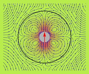
3.4. Velocity fields
Velocity fields with streamlines have been constructed over the set of squirmer types  $\beta \in \{-5,0,+5\}$ and resistances
  $R_{m}:= \{R_{\parallel },R_{\perp }\}$, for a fixed container to squirmer size ratio
  $b/a = 5$. Velocity fields for a
  $\beta = -5$ pusher,
  $\beta = 5$ puller, and
  $\beta = 0$ neutral squirmer are shown respectively in panel pairs 3(a,d), 3(b,e) and 3(c,f). The aforementioned pairs of panels are grouped by resistance parameterizations
  $R_{\parallel } < R_{\perp }$ for
  $R/a = \{10,100\}$ and
  $R_{\parallel } > R_{\perp }$ for
  $R/a = \{100,10\}$. The velocity fields are constructed in Cartesian coordinates by sweeping over the sets
  $\{\psi ^{i}(x,z,\phi ): b^{2} \ge x^{2}+z^{2} \ge a^{2}, \phi \in [0,{\rm \pi} ] \}$ and
  $\{\psi ^{e}(x,z,\phi ): x^{2}+z^{2}>b^{2}, \phi \in [0,{\rm \pi} ] \}$ and applying (3.2). Streamlines are constructed using standard formalisms.

Figure 3. Velocity fields are shown for a container to particle size ratio  $b/a = 5$, squirmer types
  $\beta \in \{-5,0,5\}$ and membrane resistance parameters
  $R_{m}=\{R_{\parallel },R_{\perp }\} = \{10,100\}$ and
  $\{100,10\}$. The centre arrow shows the squirmer's swim direction,
  $\boldsymbol {e}_{s} := \boldsymbol {e}_{z}$. The fluid velocity scales have normalized units
  $|\boldsymbol {u}(\boldsymbol {x},\boldsymbol {z})|/|\boldsymbol {U}^{sq}_{fs}|$.
Velocity fields in which  $R_{\parallel } < R_{\perp }$ show that the fluid exits preferentially in tangential directions relative to the membrane surface. Conversely the condition,
  $R_{\parallel } > R_{\perp }$ forces fluid to enter and exit the membrane with a larger normal velocity component. Although translational velocities of the squirmer and container, in the concentric geometry, are independent of the squirmer's type,
  $\beta$, the flow fields are very much dependent on
  $\beta$. Neutral squirmers are seen to produce flow fields that are similar to the source dipole flow field. Pushers tend to draw fluid in radially (relative to
  $\boldsymbol {e}_{s}$) and expel it out axially. Pullers draw fluid in axially and expel it out radially. Both pushers and pullers expel fluid asymmetrically relative to the
  $xy$-plane, and thus generate net motion along their orientation
  $\boldsymbol {e}_{s}$ (in this case in
  $+\boldsymbol {e}_{z}$). Pushers and pullers should functionally behave like the point force dipole solution of Stokes flow; however, the container induces vortical flows in both the
  $z$-anterior and
  $z$-posterior portions of the container. This phenomenon is purely of hydrodynamic origin, owing to the confinement effects of the container.
4. Boundary integral formulation
The basis for the direct boundary integral method is the integral representation (Pozrikidis Reference Pozrikidis1992; Kim & Karrila Reference Kim and Karrila2005)
 \begin{equation} \int_{\varGamma}{\mathsf{K}}_{ij}(\boldsymbol{x},\boldsymbol{y}) u_{j}(\kern1.5pt\boldsymbol{y})\,\textrm{d}S(\kern1.5pt\boldsymbol{y}) - \int_{\varGamma}{\mathsf{G}}_{ij}(\boldsymbol{x},\boldsymbol{y})\,f_{j}(\kern1.5pt\boldsymbol{y})\,\textrm{d}S(\kern1.5pt\boldsymbol{y}) = \begin{cases} 2u_{i}(\boldsymbol{x}), & \boldsymbol{x} \in \varOmega\\ 0, & \boldsymbol{x} \ne \varOmega \end{cases}, \end{equation}
where  $\boldsymbol {x}$ is a point inside the volume
  $\varOmega$,
  $\boldsymbol {u}$ is the velocity,
  $\boldsymbol {f}$ is a force density and the integrals are performed over the surface
  $\varGamma$ in the variable
  $\boldsymbol {y}$. The tensors,
  $\boldsymbol{\mathsf{K}}(\boldsymbol {x},\boldsymbol {y})$ and
  $\boldsymbol{\mathsf{G}}(\boldsymbol {x},\boldsymbol {y})$, are the double and single layer potentials for Stokes flow
 \begin{gather} {\mathsf{K}}_{ij}(\boldsymbol{x},\boldsymbol{y}) := -\frac{2}{3{\rm \pi}}\frac{(\kern1.5pt\boldsymbol{y} - \boldsymbol{x})_{i}(\kern1.5pt\boldsymbol{y} - \boldsymbol{x})_{j}(\kern1.5pt\boldsymbol{y} - \boldsymbol{x})_{k}n_{k}(\kern1.5pt\boldsymbol{y})}{|(\kern1.5pt\boldsymbol{y}-\boldsymbol{x})|^{5}}, \end{gather}
 \begin{gather}{\mathsf{G}}_{ij}(\boldsymbol{x},\boldsymbol{y}) := \frac{1}{4{\rm \pi}\mu}\left(\frac{\delta_{ij}}{|(\kern1.5pt\boldsymbol{y}-\boldsymbol{x})|} + \frac{(\kern1.5pt\boldsymbol{y}-\boldsymbol{x})_{i}(\kern1.5pt\boldsymbol{y}-\boldsymbol{x})_{j}}{|(\kern1.5pt\boldsymbol{y}-\boldsymbol{x})|^{3}}\right), \end{gather}
which differ from their classical definitions by an additional factor of two, and where  $\boldsymbol {n}(\kern1.5pt\boldsymbol {y})$ is the surface normal vector. Across a Lyapunov-smooth surface, it is well known that the single layer potential is continuous whereas the double-layer potential is discontinuous and satisfies the jump conditions (Phan-Thien & Kim Reference Phan-Thien and Kim1994; Steinbach Reference Steinbach2008)
 \begin{equation} \begin{aligned} \boldsymbol{u}^{i,e}(\boldsymbol{x}) & = \lim_{\epsilon \to 0^{+}}\boldsymbol{u}( \boldsymbol{x} \mp \epsilon \boldsymbol{n}(\boldsymbol{x}) ),\\ & ={\mp}\boldsymbol{\phi}(\boldsymbol{x}) + \int_{\varGamma}\boldsymbol{\mathsf{K}}(\boldsymbol{x},\boldsymbol{y})\boldsymbol{\phi}(\kern1.5pt\boldsymbol{y})\,\textrm{d}S(\kern1.5pt\boldsymbol{y}), \end{aligned} \quad \boldsymbol{x} \in \varGamma, \end{equation}
for an arbitrary velocity density,  $\boldsymbol {\phi }(\boldsymbol {x})$, and normal vector,
  $\boldsymbol {n}(\boldsymbol {x})$, that points into
  $\varOmega _{e}$. The integral in (4.3) should be understood as a Cauchy principal value integral, and the negative or positive sign applies when the limit is taken from the internal (
 $\varOmega _{i}$) or external (
 $\varOmega _{e}$) side of
  $\varGamma$ (Pozrikidis Reference Pozrikidis1992). Taking the limit as
  $\boldsymbol {x} \to \varGamma$ of (4.1) in the direction that the surface normal points yields the boundary integral equation (BIE)
 \begin{equation} u_{i}(\boldsymbol{x}) = \int_{\varGamma}{\mathsf{K}}_{ij}(\boldsymbol{x},\boldsymbol{y}) u_{j}(\kern1.5pt\boldsymbol{y})\,\textrm{d}S(\kern1.5pt\boldsymbol{y}) - \int_{\varGamma}{\mathsf{G}}_{ij}(\boldsymbol{x},\boldsymbol{y})\,f_{j}(\kern1.5pt\boldsymbol{y})\,\textrm{d}S(\kern1.5pt\boldsymbol{y}),\quad \boldsymbol{x} \in \varGamma, \end{equation}
where a jump of  $+\boldsymbol {u}(\boldsymbol {x})$ has been accounted for as required by (4.3). Apart from a factor of 1/2 (recall that (4.2a) and (4.2b) have been multiplied by an extra factor of two), and modulo sign conventions used in (4.2), (4.4) is the usual boundary integral equation that provides the starting point for boundary element analysis in most boundary element literature.
When solving mobility problems, the force density distribution is unknown, and (4.4) becomes an ill-posed Fredholm integral equation of the first kind. To formulate a well-posed integral equation of the second kind, the fluid velocity may instead be written in terms of the double-layer potential and an aphysical velocity density,  $\boldsymbol {\phi }(\boldsymbol {x})$, as
 \begin{equation} \boldsymbol{u}(\boldsymbol{x}) = \boldsymbol{\phi}(\boldsymbol{x}) + \int_{\varGamma}\boldsymbol{\mathsf{K}}(\boldsymbol{x},\boldsymbol{y})\boldsymbol{\phi}(\kern1.5pt\boldsymbol{y})\,\textrm{d}S(\kern1.5pt\boldsymbol{y}), \quad \boldsymbol{x} \in \varGamma. \end{equation}
It is well known that (4.5) can only describe a force- and torque-free surface. In fact, the completed double-layer boundary integral equation method (CDLBIEM) (Power & Miranda Reference Power and Miranda1987; Karrila & Kim Reference Karrila and Kim1989; Phan-Thien & Kim Reference Phan-Thien and Kim1994; Kim & Karrila Reference Kim and Karrila2005) seeks to generalize (4.5) to surfaces with finite forces and torques. However, since the squirmer is by definition force and torque free there is no need to use the full range completion terms from the original CDLBIEM method, and (4.5) is sufficient for describing the squirmer. To describe the container, the BIE in (4.1) will be used to derive a second kind integral equation that is a function of a discontinuous interfacial force.
Since the Stokes equations are linear partial differential equations, individual velocity contributions may be superimposed to construct the full velocity field. In the context of the squirmer–container geometry, the fluid velocity inside of the container may be decomposed as a sum of velocities arising from integral contributions from singularity distributions over squirmer and container surfaces. Therefore, the fluid velocity at point  $\boldsymbol {x}$ in the interior fluid region,
  $\varOmega _{i}$, may be generically written as
 \begin{equation} \boldsymbol{u}(\boldsymbol{x}) = \boldsymbol{u}^{sq}(\boldsymbol{x}) + \boldsymbol{u}^{c}(\boldsymbol{x}),\quad \boldsymbol{x} \in \varOmega_{i}. \end{equation}
It is then useful to define disturbance velocity fields  $\bar {\boldsymbol {u}}^{sq}(\boldsymbol {x})$ and
  $\bar {\boldsymbol {u}}^{c}(\boldsymbol {x})$ such that
 \begin{gather} \bar{\boldsymbol{u}}^{sq}(\boldsymbol{x}) = \boldsymbol{u}(\boldsymbol{x}) - \boldsymbol{u}^{sq}(\boldsymbol{x}), \end{gather}
 \begin{gather}\bar{\boldsymbol{u}}^{c}(\boldsymbol{x}) = \boldsymbol{u}(\boldsymbol{x}) - \boldsymbol{u}^{c}(\boldsymbol{x}). \end{gather}
Equations (4.6)–(4.8) simplify notation as they allow individual velocity contributions to be expressed relative to a disturbance velocity field.
4.1. Squirmer velocity contribution
Since the Stokes double-layer potential is able to fully represent flow fields that correspond to force- and torque-free surfaces, the double-layer potential can be used to elegantly describe the squirmer's disturbance velocity field. The squirmer's velocity contribution is formulated based on (4.5) as an indirect Fredholm integral equation of the second kind in an aphysical velocity density acting on the Stokes double-layer bivariate potential. Observing the form of (4.5) and the aforementioned jump properties of the double layer potential in (4.3), the squirmer's disturbance velocity field in (4.7) is found to be
 \begin{align} \boldsymbol{U}^{sq} + \boldsymbol{\varOmega}^{sq} \times ( \boldsymbol{x} - \boldsymbol{x}^{sq}_{c}) + \boldsymbol{u}^{sl}(\boldsymbol{x}) - \bar{\boldsymbol{u}}^{sq}(\boldsymbol{x}) = \boldsymbol{\phi}(\boldsymbol{x})\nonumber\\ + \int_{\varGamma_{sq}}\boldsymbol{\mathsf{K}}(\boldsymbol{x},\boldsymbol{y})\boldsymbol{\phi}(\kern1.5pt\boldsymbol{y})\,\textrm{d}S(\kern1.5pt\boldsymbol{y}), \quad \boldsymbol{x} \in \varGamma_{sq}, \end{align}
where the velocity boundary condition at the squirmer's surface is used in conjunction with (4.7) to couple the fluid velocity on the squirmer's surface to the squirmer's rigid body motion. The slip velocity  $\boldsymbol {u}^{sl}(\boldsymbol {x})$, defined in (2.2), is solely responsible for generating the propulsive force,
  $\boldsymbol {F}^{P}$, that drives the squirmer whereas the rigid body motion terms,
  $\boldsymbol {U}^{sq}$ and
  $\boldsymbol {\varOmega }^{sq}$, give rise to the drag force
  $\boldsymbol {F}^{D}$ from (3.15a). Although the singularity present in the kernel
  $\boldsymbol{\mathsf{K}}$ is proportional to
  $1/r^{2}$, (4.9) is a second kind integral equation and admits rigorous analysis under the Fredholm–Riesz–Schauder theory (Hsiao & Wendland Reference Hsiao and Wendland2008; Kress Reference Kress2014) so long as the surface is sufficiently smooth.
Using the CDLBIEM completion relationships (Karrila & Kim Reference Karrila and Kim1989; Kim & Karrila Reference Kim and Karrila2005)
 \begin{gather} \boldsymbol{U}^{sq} ={-} \sum_{j=1}^{3}\boldsymbol{\varphi}^{j,RBM}(\boldsymbol{x})\langle\boldsymbol{\varphi}^{j,RBM}, \boldsymbol{\phi} \rangle, \end{gather}
 \begin{gather}\boldsymbol{\varOmega}^{sq} \times( \boldsymbol{x} - \boldsymbol{x}_{c}^{sq}) ={-} \sum_{j=4}^{6}\boldsymbol{\varphi}^{j,RBM}(\boldsymbol{x})\langle \boldsymbol{\varphi}^{j,RBM},\boldsymbol{\phi} \rangle, \end{gather}
where  $\boldsymbol {x}_{c}^{sq}$ is the squirmer's centroid, (4.9) may be written solely in terms of the velocity potential
  $\boldsymbol {\phi }$. The,
  $\boldsymbol {\varphi }^{i,RBM}, i \in \{1,\ldots ,6\}$, are the rigid body motion (RBM) eigenfunctions of the homogeneous form of (4.3) with eigenvalue –1, which are proportional to
  $\boldsymbol {e}_{x}, \boldsymbol {e}_{y}, \boldsymbol {e}_{z}$,
  $\boldsymbol {e}_{x} \times (\boldsymbol {x} - \boldsymbol {x}_{c}^{sq})$,
  $\boldsymbol {e}_{y} \times (\boldsymbol {x} - \boldsymbol {x}_{c}^{sq})$ and
  $\boldsymbol {e}_{z} \times (\boldsymbol {x} - \boldsymbol {x}_{c}^{sq})$. In practice, when dealing with a mesh approximation to
  $\varGamma _{sq}$, these functions are numerically determined by making them orthonormal with respect to the natural inner product norm on the surface
 \begin{equation} \langle \boldsymbol{a}, \boldsymbol{b} \rangle = \int_{\varGamma_{sq}}a_{i}(\boldsymbol{x})b_{i}(\boldsymbol{x})\,\textrm{d}S(\boldsymbol{x}), \end{equation}
using the modified Gram–Schmidt process. For a perfectly spherical surface they take the forms (Phan-Thien & Kim Reference Phan-Thien and Kim1994)
 \begin{gather} \boldsymbol{\varphi}^{i,RBM}(\boldsymbol{x}) = \frac{1}{\sqrt{|\varGamma_{sq}|}}\boldsymbol{e}_{i}, \end{gather}
 \begin{gather}\boldsymbol{\varphi}^{i+3,RBM}(\boldsymbol{x}) = \frac{1}{\sqrt{I_{i}}}\boldsymbol{e}_{i} \times (\boldsymbol{x} - \boldsymbol{x}^{sq}_{c}), \end{gather}
where  $|\varGamma _{sq}|$ is the surface area of the squirmer and
 \begin{equation} I_{i} = \int_{\varGamma_{sq}}\left[ (\kern1.5pt\boldsymbol{y}-\boldsymbol{x}^{sq}_{c})\boldsymbol{\cdot} (\kern1.5pt\boldsymbol{y}-\boldsymbol{x}^{sq}_{c}) - (\kern1.5pt\boldsymbol{y}-\boldsymbol{x}^{sq}_{c})_{i}^{2} \right] \,\textrm{d}S(\kern1.5pt\boldsymbol{y} ), \quad i \in \{1,\ldots,3\}, \end{equation}
are the surface moments.
Substituting (4.10) and (4.11) into (4.9) results in
 \begin{equation} \boldsymbol{u}^{sl}(\boldsymbol{x}) - \bar{\boldsymbol{u}}^{sq}(\boldsymbol{x}) = \boldsymbol{\phi}(\boldsymbol{x}) + \int_{\varGamma_{sq}}\boldsymbol{\mathsf{K}}(\boldsymbol{x},\boldsymbol{y})\boldsymbol{\phi}(\kern1.5pt\boldsymbol{y})\,\textrm{d}S(\kern1.5pt\boldsymbol{y})\nonumber\\ + \sum_{j=1}^{6}\boldsymbol{\varphi}^{j,RBM}(\boldsymbol{x})\langle \boldsymbol{\varphi}^{j,RBM}, \boldsymbol{\phi} \rangle, \end{equation}
where the integral equation's eigenvalue at  $-1$ of rank six, corresponding to the operator
  $(\mathbb {I} + \mathcal {K})$, is mapped to zero. After solving for
  $\boldsymbol {\phi }$, post processing with the completion relations, (4.10) and (4.11), allows for recovery of
  $\boldsymbol {U}^{sq}$ and
  $\boldsymbol {\varOmega }^{sq}$.
4.2. Container velocity contribution
In formulating the container contribution, explicit indications of where  $\boldsymbol {x}$ and
  $\boldsymbol {y}$ are located are made relative to the defined container normal vector,
  $\boldsymbol {n}$. Since the container normal points exterior to the container, quantities that depend on points
  $\boldsymbol {x}$ and
  $\boldsymbol {y}$ in
  $\varOmega _{e}$ and in the direction of
  $\boldsymbol {n}$, are denoted with a superscript
  $+$. Similarly, quantities that depend on
  $\boldsymbol {x}$ and
  $\boldsymbol {y}$ in volume
  $\varOmega _{i}$ bounded by
  $\varGamma _{c-}$, are denoted with a superscript
  $-$.
$-$.
Under zero viscosity contrast inside and outside of the container, the Stokes boundary integral equations in the primary variables (surface velocities  $\boldsymbol {u}(\boldsymbol {x})$ and tractions
  $\boldsymbol {f}(\boldsymbol {x})$) may be applied to both sides of the container to find that
 \begin{align}
\boldsymbol{u}^{c}(\boldsymbol{x}) -
\bar{\boldsymbol{u}}^{c}(\boldsymbol{x}) &= \left[
\boldsymbol{u}^{+}(\boldsymbol{x}) -
\boldsymbol{u}^{-}(\boldsymbol{x}) \right] +
\int_{\varGamma_{c}}\boldsymbol{\mathsf{K}}(\boldsymbol{x},\boldsymbol{y})
\left[ \boldsymbol{u}^{+}(\kern1.5pt\boldsymbol{y}) -
\boldsymbol{u}^{-}(\kern1.5pt\boldsymbol{y})\right]\,\textrm{d}S(\kern1.5pt\boldsymbol{y})\nonumber\\
&\quad - \tfrac{1}{2}\int_{\varGamma_{c}}\boldsymbol{\mathsf{G}}(\boldsymbol{x},\boldsymbol{y})
\left[ \boldsymbol{f}^{+}(\kern1.5pt\boldsymbol{y}) -
\boldsymbol{f}^{-}(\kern1.5pt\boldsymbol{y})
\right]\,\textrm{d}S(\kern1.5pt\boldsymbol{y}),
\end{align}
\begin{align}
\boldsymbol{u}^{c}(\boldsymbol{x}) -
\bar{\boldsymbol{u}}^{c}(\boldsymbol{x}) &= \left[
\boldsymbol{u}^{+}(\boldsymbol{x}) -
\boldsymbol{u}^{-}(\boldsymbol{x}) \right] +
\int_{\varGamma_{c}}\boldsymbol{\mathsf{K}}(\boldsymbol{x},\boldsymbol{y})
\left[ \boldsymbol{u}^{+}(\kern1.5pt\boldsymbol{y}) -
\boldsymbol{u}^{-}(\kern1.5pt\boldsymbol{y})\right]\,\textrm{d}S(\kern1.5pt\boldsymbol{y})\nonumber\\
&\quad - \tfrac{1}{2}\int_{\varGamma_{c}}\boldsymbol{\mathsf{G}}(\boldsymbol{x},\boldsymbol{y})
\left[ \boldsymbol{f}^{+}(\kern1.5pt\boldsymbol{y}) -
\boldsymbol{f}^{-}(\kern1.5pt\boldsymbol{y})
\right]\,\textrm{d}S(\kern1.5pt\boldsymbol{y}),
\end{align}
where  $\boldsymbol {u}^{c}(\boldsymbol {x})$ is the fluid velocity evaluated on the container/membrane surface. This fluid velocity is different from the membrane's physical point-wise velocity,
  $\boldsymbol {u}^{m}(\boldsymbol {x})$, unless no slip is used in conjunction with the standard kinematic boundary condition. The fluid velocity is assumed to be continuous across the membrane, as would be the case for pressure driven flow through a cylindrical pore (i.e. fully developed Hagen–Poiseuille flow). Imposing this condition as
  $\boldsymbol {u}^{+}(\boldsymbol {x}) = \boldsymbol {u}^{-}(\boldsymbol {x})$, (4.16) reduces to
 \begin{equation} \boldsymbol{u}^{c}(\boldsymbol{x}) - \bar{\boldsymbol{u}}^{c}(\boldsymbol{x}) ={-}\tfrac{1}{2}\int_{\varGamma_{c}}\boldsymbol{\mathsf{G}}(\boldsymbol{x},\boldsymbol{y}) \left[ \boldsymbol{f}^{+}(\kern1.5pt\boldsymbol{y}) - \boldsymbol{f}^{-}(\kern1.5pt\boldsymbol{y}) \right]\,\textrm{d}S(\kern1.5pt\boldsymbol{y}). \end{equation}
To proceed with modelling the squirmer–container system, a constitutive law, analogous to (3.23) and (3.20), is needed to describe the stress jump across the membrane. The jump in stress is modelled as
 \begin{align} \Delta \boldsymbol{f}(\kern1.5pt\boldsymbol{y}) &:= \left[ \boldsymbol{f}^{+}(\kern1.5pt\boldsymbol{y}) - \boldsymbol{f}^{-}(\kern1.5pt\boldsymbol{y}) \right],\nonumber\\ &={-}\left[ \boldsymbol{f}^{b}(\kern1.5pt\boldsymbol{y}) + \boldsymbol{f}^{\gamma}(\kern1.5pt\boldsymbol{y}) + \boldsymbol{f}^{p}(\kern1.5pt\boldsymbol{y})\right], \end{align}
which includes forces related to membrane bending  $\boldsymbol {f}^{b}$, tension
  $\boldsymbol {f}^\gamma$ and resistance to permeable flow
  $\boldsymbol {f}^{p}$. In the present model the membrane is rigid and can only support a permeable force density expressed as
 \begin{align} \boldsymbol{f}^{p}(\kern1.5pt\boldsymbol{y}) &={-}\left[ \boldsymbol{u}^{c}(\kern1.5pt\boldsymbol{y})-\boldsymbol{u}^{m}(\kern1.5pt\boldsymbol{y}) \right ] \boldsymbol{\cdot} \left[ R_{n}\boldsymbol{n}(\kern1.5pt\boldsymbol{y})\boldsymbol{n}(\kern1.5pt\boldsymbol{y}) + R_{b}\boldsymbol{b}(\kern1.5pt\boldsymbol{y})\boldsymbol{b}(\kern1.5pt\boldsymbol{y}) + R_{t}\boldsymbol{t}(\kern1.5pt\boldsymbol{y})\boldsymbol{t}(\kern1.5pt\boldsymbol{y}) \right],\nonumber\\ &={-}\left\{ \boldsymbol{u}^{c}(\kern1.5pt\boldsymbol{y})-\left[ \boldsymbol{U}^{m} + \boldsymbol{\varOmega}^{m} \times (\kern1.5pt\boldsymbol{y} - \boldsymbol{x}^{c}_{c})\right] \right \}\nonumber\\ &\quad \boldsymbol{\cdot} \left\{ R_{n}\boldsymbol{n}(\kern1.5pt\boldsymbol{y})\boldsymbol{n}(\kern1.5pt\boldsymbol{y}) + R_{b}\boldsymbol{b}(\kern1.5pt\boldsymbol{y})\boldsymbol{b}(\kern1.5pt\boldsymbol{y}) + R_{t}\boldsymbol{t}(\kern1.5pt\boldsymbol{y})\boldsymbol{t}(\kern1.5pt\boldsymbol{y}) \right\}. \end{align}
This model is equivalent to the analytical formulation under the identifications  $R_{\perp } := R_{n}$,
  $R_{\parallel } := R_{b} = R_{t}$. The vectors
  $\boldsymbol {t},\boldsymbol {b},\boldsymbol {n}$ are respectively the tangent, bitangent and normal vectors and provide a localized point-wise tangent space on the container's surface.
In addition, integral constraints on the total hydrodynamic force and torque on the membrane container must be made to fix the system
 \begin{gather} \int_{\varGamma_{c}}\Delta \boldsymbol{f}(\kern1.5pt\boldsymbol{y})\,\textrm{d}S(\kern1.5pt\boldsymbol{y}) = \boldsymbol{F}^{H} = \boldsymbol{0}, \end{gather}
 \begin{gather}\int_{\varGamma_{c}} (\kern1.5pt\boldsymbol{y} - \boldsymbol{x}_{c}^{c}) \times \Delta \boldsymbol{f}(\kern1.5pt\boldsymbol{y})\,\textrm{d}S(\kern1.5pt\boldsymbol{y}) = \boldsymbol{T}^{H} = \boldsymbol{0}, \end{gather}
where  $\boldsymbol {x}_{c}^{c}$ is the container's centroid, and
  $\boldsymbol {F}^{H}$ and
  $\boldsymbol {T}^{H}$ are the hydrodynamic force and torque acting on the container.
5. Results
The numerical solution to the coupled set of boundary integral equations, (4.15) and (4.17), subject to the constraints, (4.20) and (4.21), is computed over a range of container–particle size ratios of  $b/a \in \{1.05, \ldots , 10\}$ and maintains accuracy by using adaptive mesh refinement. Additional details relevant to the numerical discretization, assembly of the global linear system and mesh adaptivity algorithm may be found in both appendix B and Marshall (Reference Marshall2018). In brief summary, the weak forms of both BIEs are constructed and solved over discrete triangular mesh decompositions of the surfaces
  $\varGamma _{sq}$ and
  $\varGamma _{c}$. Mesh adaptivity is maintained in near surface-to-surface contact regions using a conformal
  $h$-adaptive meshing algorithm that extends the newest vertex bisection (NVB) method of Mitchell (Reference Mitchell1989). The linear system is solved using an in-house Galerkin boundary element method (GBEM) implementation called GPU-GBEM that runs on CUDA enabled GPUs. This implementation has been created as a general framework for solving a wide variety of multi-body fluid–structure interaction problems in Stokes flow. The GPU-GBEM framework maps GBEM calculations and assembly routines onto the GPU using analogous implementations of the well-known fast-nbody simulation techniques (Nguyen Reference Nguyen2007). Issues related to race conditions, data partitioning and thread concurrency all manifest and may be dealt with using standard methods.
5.1. Numerical comparison with the analytical model
The analytical solutions in (3.27) and (3.28) are compared with the GBEM numerics in figures 4 and 5 when the container's and squirmer's centres of mass are coincident. This comparison is made for a variety of confinement ratios  $b/a > 1$, resistance parameter sets
  $R=\{R_{\parallel },R_{\perp }\}$, and squirmer types (defined by
  $\beta = B^{sq}_{2} / B^{sq}_{1}$). So long as the number of nodes is kept relatively small, the solution of the linear system may be obtained using standard LU decomposition. Situations in which
  $b/a \approx 1$ or where
  $(b-a)/a \approx \delta$ for
  $\delta \ll 1$ require one to use either mesh adaptivity and/or efficient nearly singular quadratures to control element size and errors in numerical integrations.

Figure 4. The non-dimensional centre of mass translational speed of a  $\beta =5$ squirming particle (see (3.27)) is plotted as a function of the container–particle size ratio,
  $b/a$ for various sets of membrane resistance parameters
  $R_{m} = \{R_{\parallel },R_{\perp }\}$. Numerical solutions obtained by solving (B35) are shown with symbols. For a concentric squirmer–container configuration the squirmer's velocity is independent of the second squirming mode
  $B^{sq}_{2}$ which indicates that all types of squirmers (pusher, puller, neutral) move with the same velocity.

Figure 5. The non-dimensional centre of mass translational speed of the porous container (see (3.28)) is plotted as a function of the container–particle size ratio,  $b/a$ for various sets of membrane resistance parameters
  $R_{m} = \{R_{\parallel },R_{\perp }\}$. For a concentric squirmer–container configuration the container's velocity is independent of the squirmer's type but dependent on the sign of the quantity
  $R_{\perp } - R_{\parallel }$.
The resistance parameters  $R_{m}=\{R_{\parallel },R_{\perp }\}$ have units
  $1/L$ and so membrane resistances in all plots are non-dimensionalized by multiplying with the particle size
  $a$. When there is relatively weak resistance to normal permeable flow through the membrane,
  $R_{\parallel } > R_{\perp }$, the squirmer moves opposite to the membrane. However, when
  $R_{\parallel } < R_{\perp }$ and tangential flow through the membrane is favoured, the membrane and squirmer both move in the same direction. In the situation where
  $R_{\parallel } < R_{\perp }$, flow across the membrane is primarily in the tangential direction and almost exactly mirrors the squirmer's tangential slip boundary condition. The squirmer is able to transmit its slip boundary condition onto the container's surface by forming recirculating vortical flows which extend out beyond the container's surface. This effectively turns the container into a larger version of a tangential squirmer. On the other hand, when there is weak resistance to normal permeable flow, the squirmer always pushes a net volume of fluid behind its body. Consequently, the passive porous container, which now allows this fluid to flow through its surface in the normal direction, is convected backwards with this net fluid motion. These effects are seen more clearly in the velocity fields from § 3.4.
In the limit that  $\{R_{\parallel },R_{\perp }\} \to \{\infty ,\infty \}$, the numerical calculations show agreement with the analytical non-porous container solution, (3.18). Additionally, the numerically calculated
  $\boldsymbol {U}^{sq}$ shows a global minimum that is in agreement with the analytic model. This minimum is at a particular size ratio where the squirmer moves the slowest, and is understood as a confinement effect where the squirmer becomes inefficient at moving fluid tangentially around its body. Both
  $\boldsymbol {U}^{sq}$ and
  $\boldsymbol {U}^{m}$ decay respectively to the free space squirming velocity,
  $2/3 B^{sq}_{1} \boldsymbol {e}_{z}$, and
  $\boldsymbol {0}$ as
  $b/a \to \infty$. Similar plots (not shown) have been constructed for a wider variety of resistances, and show in general that a higher resistance leads to slower squirmer and container translational speeds.
5.2. Mobility fields
Squirmer and container trajectories may be simulated by integrating the solutions to the mobility problem, (B35), over time. However, instead of solving the quasi-static mobility problem separately at each point in time, mobility solutions are obtained using interpolation over a special set of standard mobility solutions. A standard mobility solution is defined as a solution to the squirmer porous container problem under a standard parameterization
 \begin{equation} \boldsymbol{P}^{0}(x,z) = \langle a,b,R_{t},R_{b},R_{n},B^{sq}_{1},B^{sq}_{2},\boldsymbol{e}_{s}=\boldsymbol{e}_{z},\boldsymbol{x}_{c}^{sq}=(x,0,z),\boldsymbol{x}_{c}^{c}=(0,0,0)\rangle. \end{equation}
Solutions to the mobility problem are obtained at regularly spaced parameterizations  $\boldsymbol {P}^{0}(x,z)$ on a circularly masked Cartesian grid in the region defined by
 \begin{equation} r_{cp} := |\boldsymbol{x}_{c}^{sq} - \boldsymbol{x}_{c}^{c}| < b - a(1+\delta) =: r^{max}_{cp}, \end{equation}
where  $\delta$ is a fractional container to squirmer gap size.
Figures 6 and 7 show the translational velocity mobility fields for the squirmer and container. Point-wise vectors indicate the velocity of either the squirmer or container if the squirmer were located at the corresponding point. In all of the following trajectory and mobility field calculations, computations are performed down to  $\delta = 0.05$. Owing to the fact that it is physically impossible for a squirmer to pass through the container surface, a simple collision model is used where squirmers attempting to cross the container boundary remain fixed at a centre to centre separation of
  $r^{max}_{cp}$, yet may continue to keep running into the container boundary at the
  $\delta = 0.05$ level mobility solution.

Figure 6. The translational container velocity,  $\boldsymbol {U}^{m}$, is plotted for parameterizations
  $\boldsymbol {P}^{0}(x,z)$ with
  $b/a = 5$. Panels (a–c and d–f) show results for resistances where either
  $R_{\parallel } < R_{\perp }$ or
  $R_{\parallel } > R_{\perp }$ for
  $\{R_{\parallel },R_{\perp }\} = \{10,100\}$. Panels (a,d), (b,e) and (c,f) are grouped by squirmer type. The black, red, pink and grey circles give notions of regions where
  $r=b$,
  $r=b-a\delta$,
  $r=r_{cp}^{max}$ and
  $r=a$ respectively.

Figure 7. The translational squirmer velocity,  $\boldsymbol {U}^{sq}$, is plotted for parameterizations
  $\boldsymbol {P}^{0}(x,z)$. Figures are grouped to correspond with figure 6 using the same resistance parameters and squirmer types.
5.2.1. Effect of container resistances on  $\boldsymbol {U}^{m}$ and $\boldsymbol {U}^{sq}$


Variations in the container resistance parameters have the most striking effect on the container velocity  $\boldsymbol {U}^{m}$. If the squirmer type is held constant, cases
  $R_{\parallel } > R_{\perp }$ and
  $R_{\parallel } < R_{\perp }$, approximately differ by a mirror flipping of the container velocity across both the
  $xy$- and
  $yz$-planes. This effect is shown in figure 6 for panel pairs (a,d), (b,e) and (c,f) and exists for all tested size ratios and squirmer types. This indicates that the directed motion of the porous container may be changed by modifying its intrinsic porous structure so that either normal or tangential flow through the container's surface is favoured.
Effects on the squirmer's translational velocity are less dramatic. Figure 7(a,b) shows that weak tangential resistance to permeable flow ( $R_{\parallel } < R_{\perp }$) results in weak (small magnitude) swimming near the anterior and posterior part (relative to
  $\boldsymbol {e}_{z}$) of the region defined by
  $r = r_{cp}^{max}$ for respectively
  $\beta = -5$ and
  $\beta =+5$. The swimming direction is reversed in these regions, and this causes pullers to remain trapped towards the posterior of the container. Conversely weak normal resistance to permeable flow (
 $R_{\parallel } > R_{\perp }$) does not significantly affect the overall swimming direction or magnitude to the same degree, although different types of squirmers still produce fundamentally different velocity fields.
5.2.2. Effect of squirmer type on $\boldsymbol {U}^{m}$ and $\boldsymbol {U}^{sq}$


Holding the resistance parameters fixed, each squirmer type (pusher, puller, neutral) produces a different mobility velocity field. In general,  $\beta < 0$ pushers produce
  $\boldsymbol {U}^{sq}$ mobility fields that show net motion directed upwards and radially outwards relative to the
  $z$-axis towards
  $r=r_{cp}^{max}$. Mirror symmetry exists across the
  $yz$-plane. Pullers with
  $\beta > 0$ also show net motion upwards with mirror symmetry across the
  $yz$-plane, but on the contrary, their velocity is directed radially inward towards the
  $z$-axis. A neutral squirmer creates a mostly uniform mobility field which indicates that it is relatively unaffected by the presence of the container. This distinction in how squirmers move radially outward or inwards relative to the
  $z$-axis may be further understood by examining squirmer angular velocities. Squirmer angular velocities (not shown) are directed along
  $\boldsymbol {e}_{y}$ and are anti-parallel relative to the
  $yz$-plane. The angular velocity of pushers causes net rotation in the squirmer's swim orientation away from the
  $yz$-plane. Conversely, the angular velocity of pullers causes net rotation towards the
  $yz$-plane.
The container velocity field shows a similar mirror symmetry reversal as was observed when switching from weak normal to weak tangential resistances. However, this time the mirror symmetry flipping of  $\boldsymbol {U}^{m}$ across the
  $xy$- and
  $yz$-planes is caused by changes in
  $\beta = 5 \to -5$. This implies a second mechanism for controlling the directed motion of a container – the translational motion of the container may be reversed by changing the squirmer's type from a pusher to a puller.
5.3. Trajectory analysis
Simulating squirmer and container trajectories requires solving the mobility problem at arbitrary squirmer positions and orientations. Due to the symmetry of the squirmer–container geometry, arbitrary mobility solutions may be expressed as affine transformations of the standard mobility solutions. To find the mobility solution for a squirmer with arbitrary position and orientation, several rotation matrices are needed to relate the squirmer's position and orientation to a standard mobility solution at some  $\boldsymbol {r}^{sq,xz}_{0} = \boldsymbol {x}_{c}^{sq} - \boldsymbol {x}_{c}^{c} \in \boldsymbol {P}^{0}(x,z)$. The needed rotation matrices are
  $\boldsymbol{\mathsf{R}}_{\boldsymbol {r}^{sq}}^{\boldsymbol {r}^{sq,xz}}$ which rotates
  $\boldsymbol {r}^{sq} = \boldsymbol {x}^{sq}_{c} - \boldsymbol {x}_{c}^{c}$ into the
  $xz$-plane,
  $\boldsymbol{\mathsf{R}}_{\boldsymbol {e}_{s}}^{\boldsymbol {e}_{s}^{xz}}$ which rotates the squirmer's orientation
  $\boldsymbol {e}_{s}$ into the
  $xz$-plane and
  $\boldsymbol{\mathsf{R}}_{\boldsymbol {e}^{xz}_{s}}^{\boldsymbol {e}^{z}_{s}}$ which transforms
  $\boldsymbol {e}_{s}^{xz} \to \boldsymbol {e}_{s}^{z}$. Then, by transforming
  ${\boldsymbol {r}^{sq} \to \boldsymbol {r}_{0}^{sq} = \boldsymbol{\mathsf{R}}_{\boldsymbol {e}^{xz}_{s}}^{\boldsymbol {e}^{z}_{s}}\boldsymbol{\mathsf{R}}_{\boldsymbol {r}^{sq}}^{\boldsymbol {r}^{sq,xz}} \boldsymbol {r}^{sq}}$, the squirmer's reference position,
  $\boldsymbol {r}_{0}^{sq,xz}$, in
  $\boldsymbol {P}_{k}^{0}$, may be found. Bicubic interpolation is then used to find the standard mobility solution at
  $\boldsymbol {r}_{0}^{sq,xz}$. Centred difference approximations are used to approximate first derivatives in
  $x$ and
  $y$ of the container's and squirmer's centre of mass velocities and angular velocities. To recover the actual mobility solution for a squirmer at an arbitrary position and orientation, the interpolated standard mobility is rotated back by the inverse of the rotation that was used to transform
  $\boldsymbol {e}_{s} \to \boldsymbol {e}_{z}$.
Squirmer and container trajectory plots are shown in figures 8 and 9 for a container–particle size ratio of  $b/a = 5$. Squirmer trajectories are shown in a coordinate frame that moves with the container, and container trajectories are shown in world space coordinates. Trajectories are simulated over a run time
  $t_{run} = a/|\boldsymbol {U}^{sq}_{fs}|$ from which a total simulation time may be calculated as
  $t_{tot} = t_{run} b/a$. This total time is roughly the time that it takes the squirmer to move a distance
  $b$. Since the squirmer's translational velocity is bounded above by
  $\boldsymbol {U}^{sq}_{fs}$, simulations are run for a constant multiple of
  $t_{run}$ so that the squirmer has a chance to run across the container.

Figure 8. Several squirmer trajectories are shown for various squirmer types  $\beta \in \{-5,5,0\}$ at different starting positions in the posterior part of the container. Figures are grouped to correspond with figure 7 using the same resistance parameters and squirmer types. Each squirmer is initialized with
  $\boldsymbol {e}_{s} = \boldsymbol {e}_{z}$.

Figure 9. Several container trajectories are shown for various squirmer types  $\beta \in \{-5,5,0\}$ with trajectory colours corresponding to squirmer positions from figure 8. Figures are grouped to correspond with figure 7 using the same resistance parameters and squirmer types. The container is initialized to start at
  $\boldsymbol{x}^{c}_{c} = \boldsymbol {0}$.
5.3.1. Squirmer trajectories
In a container with weak tangential resistance to permeable flow,  $R_{\parallel } < R_{\perp }$, (figure 8a–c) pullers (
 $\beta > 0$) tend to move radially inwards relative to their initial orientation, which in these simulations is
  $\boldsymbol {e}_{s}=\boldsymbol {e}_{z}$. Conversely, pushers (
 $\beta < 0$) tend to move radially outwards as they swim upwards in
  $z$. Neutral squirmers (
 $\beta = 0$) swim along relatively straight trajectories. Viewed differently, pushers tend to be attracted towards the container's surface and pullers tend move away from the container's surface. Since pushers draw fluid in radially relative to their squirming direction and expel the fluid out in the axial direction (see figure 3a,d), they tend to pull themselves towards the container's surface. Conversely, pullers draw fluid in axially and expel the fluid out radially which tends to have a centring effect on their trajectories (see figure 3b,e).
For a container with weak tangential resistance to permeable flow, there exists certain starting positions where a puller may become hydrodynamically trapped, and be unable to swim away from its initial position relative to the container. These initial trapping positions can be seen in figure 8(b) near  $(0,0,-b)$. The puller's velocity reverses sign in this region forcing it to swim towards the container's surface. Above a certain initialization point in
  $z$, all pullers are able to completely translocate to the other side of the container. Once at the container's surface, they proceed to slide inward along the container surface and migrate towards
  $(0,0,\pm b)$ in the
  $\boldsymbol {P}^{0}$ parameterization. On the other hand, pushers, in containers with weak tangential resistance to flow (figure 8a), nearly all successfully translocate several run lengths across the container. However, all pusher trajectories tend to move away from
  $(0,0,+b)$ towards radial regions that are symmetric with respect to the
  $yz$-plane. Neutral squirmers migrate towards
  $(0,0,+b)$ behaving like pullers but avoid hydrodynamic trapping.
For a container with weak normal resistance to permeable flow,  $R_{\parallel } > R_{\perp }$, (figure 8d–f) all starting positions of pullers are able to completely translocate across the container. All puller trajectories end up colliding with the container's surface and move towards
  $(0,0,+b)$. Pusher trajectories show more radial spread and move away from the
  $z$-axis, although this time at more acute angles relative to the
  $yz$-plane. Additionally, all pushers are able to completely translocate across the container. Neutral squirmers again show a relatively straight trajectory and all migrate towards
  $(0,0,+b)$.
5.3.2. Container trajectories
A permeable container gives rise to a finite container velocity and net container motion. The trajectory plots shown in figure 9 serve to illustrate the unique, often non-monotonic motion of the container. In the subsequent discussion, parallel swimming or co-swimming means that the container and squirmer both end up moving a net-positive distance in the sense that they both move upwards in  $z$ in world coordinates. Anti-parallel swimming means that the container either moves a net-negative or net-positive distance, and the squirmer respectively either swims a net-positive or net-negative distance. These notions of co-swimming and anti-parallel swimming are to be understood only up to the point where the squirmer's motion stagnates near the container boundary.
General trends which influence net container parallel swimming or anti-parallel swimming can be observed by examining the net displacement of the container. Net container and squirmer swimming directions are summarized in table 1. For weak normal permeable flow, container trajectory plots show that pullers induce net anti-parallel swimming of the container. Pushers on the other hand, induce co-swimming. Even though the container trajectories are non-monotonic, the net motion is monotonic across all studied resistance parameterizations and squirmer types. Neutral squirmers always induce anti-parallel swimming of the container. Pullers will always translocate across the container the fastest since they enjoy the added benefit of net-negative container swimming distances.
Table 1. Net squirmer and container swimming directions are shown for the  $\boldsymbol {P}^{0}$ parameterization relative to
  $\boldsymbol {e}_{z}$. An up arrow
  $\uparrow$ indicates net motion in
  $\boldsymbol {e}_{z}$. A down arrow,
  $\downarrow$, indicates net motion in
  $-\boldsymbol {e}_{z}$. The first and second arrows represent the net directional motion of the squirmer and container, respectively. Arrows are to be understood as the overall direction of the net motion of the squirmer and container for sufficiently long trajectories.

For weak tangential flow, the situation is more complex. Pullers now induce co-swimming of the container except when initialized at a hydrodynamically trapping position. Several of the squirmer positions that are very near the container's posterior relative to a squirmer orientation of  $\boldsymbol {e}_{s} = \boldsymbol {e}_{z}$ result in container co-swimming in the
  $-\boldsymbol {e}_{z}$ direction, although some positions give rise to net anti-parallel swimming. Pushers always induce anti-parallel swimming of the container. Neutral squirmers always show co-swimming of the container.
6. Conclusion
The dynamics of an active squirming particle inside of a rigid container is both rich and complex. In this paper we analysed this system starting with a static fluid mechanical analysis of a concentric squirmer–container geometry. The locomotion of the squirmer was first studied in the context of a non-porous rigid container. An exact analytical solution for the translational velocity of the squirmer was derived and compared with the solution for a forced particle moving inside of an identical container. When compared with the velocity of the forced particle, the velocity of the squirmer was seen to be much less influenced by the hydrodynamic confinement effects of the surrounding container. This phenomenon is attributed to the fact that the velocity field associated with a squirmer decays more rapidly in free space ( $\propto 1/r^{2,3}$) than the point force free space solution (
 $\propto 1/r$), and so the squirmer will tend to move in a less hindered manner sooner than the forced particle as
  $b/a \to \infty$.
A new model was proposed for describing fluid flow across a thin porous rigid container. The underlying basis of this model is Darcy's law, but this porous container model is more general and also allows for discontinuous jumps in both the normal and tangential fluid stresses across the membrane. This porous container model was solved exactly for the concentric squirmer–container geometry under a membrane resistance coefficient parameterization,  $R_{\parallel }$ and
  $R_{\perp }$, that controls how fluid passes through the container's surface. For all resistance combinations,
  $\{R_{\parallel },R_{\perp }\}$, there exists a global minimum value in the squirmer's translational velocity at a particular size ratio
  $(b/a)_{min}$. This was understood as the size ratio where the squirmer becomes the most inefficient at moving fluid through the container's surface. Velocity flow fields with streamlines for the squirmer and porous container were generated from the exact analytical solutions. Each flow field was seen to be heavily influenced by the squirmer type
  $\beta$. Pushers, defined by
  $\beta < 0$, tend to draw fluid in along the radial direction and expel it out axially relative to the squirmer's orientation,
  $\boldsymbol {e}_{s}$. They do so asymmetrically so as to push more net flow towards
  $-\boldsymbol {e}_{z}$ thereby generating net thrust in
  $\boldsymbol {e}_{z}$. Pullers, defined by
  $\beta > 0$, swim by a different mechanism, and tend to draw fluid in axially relative to
  $\boldsymbol {e}_{s}$ and expel it out radially. Again, this is performed asymmetrically so as to generate net thrust in
  $\boldsymbol {e}_{z}$. Pushers and pullers were seen to both create vortical flows in the axial
  $z$-anterior and
  $z$-posterior portions of the container. This effect is purely of hydromechanical origin. These vortical flows hydrodynamically transmit the container's slip velocity to the container's walls thereby causing the container to swim.
Next, a coupled set of boundary integral equations were derived for describing the squirmer and porous container. A completed double-layer boundary integral representation was used to described the squirmer's fluid dynamics. Since the squirmer is by definition, a force- and torque-free body, it can be perfectly represented by the Stokes BIE operator  $\mathcal {K}$. The container BIE representation was expressed using a Stokes single layer potential with operator,
  $\mathcal {G}$, acting on a surface traction discontinuity
  $\Delta \boldsymbol {f}$. This term was written using the newly proposed porous membrane model. The porous container's resistances were generalized under the identification
  $R_{m} = \{R_{t},R_{b},R_{n}\} = \{R_{\parallel },R_{\parallel },R_{\perp }\}$ with tangent, bitangent and normal permeable resistances given respectively by
  $R_{t},R_{b},R_{n}$. This description of the container yielded a second kind BIE equation making the overall description of the coupled system second kind although with container force- and torque-free constraints.
The coupled system of boundary integral equations describing the dynamics of the porous container and squirmer system was discretized using the Galerkin method. While this discretization method has been well known since the inception of the finite element method, its application to BEM and multi-body hydrodynamics problems is relatively unexplored. The squirmer porous container problem was solved under this discretization using the GPUGBEM framework. All boundary element calculations were performed on CUDA-enabled GPUs. Accuracy in all calculations was maintained using an adaptive local refinement algorithm that preserves the mesh manifold property, and thus global  $C^{0}$ continuity of all underlying unknown boundary datums.
Numerical solutions were obtained for the perfectly concentric geometry, and were found to be in excellent agreement with the exact analytical model. The squirmer's translational velocity was seen to be bounded below by the solution for the non-porous container. Global minima in the squirmer's velocity, present in the analytical model, were recovered in the GBEM numerics.
In order to fully characterize the squirmer's and container's dynamics, a trajectory analysis was performed using an interpolation procedure. An important symmetry observation of the system was made, namely that the container and squirmer always share a symmetry plane that contains both of their individual centres of mass, and that the mobility solution is only unique up to how the squirmer is oriented. If the fluid mechanics can be resolved in this single plane at a standard squirming orientation, then the fluid mechanics is known in all space up to an affine transformation. Knowing the mobility solution up to an affine transformation allowed for the fast simulation and calculation of trajectories for arbitrary squirmer orientations and positions. The planar grid containing all the relevant fluid mechanics information was referred to as a mobility solution field. Mobility solution fields were constructed in a standard but arbitrary reference configuration, namely the  $xz$-plane, and with a standard squirmer orientation
  $\boldsymbol {e}_{z}$. Mobility solution fields were used to interpolate squirmer and container trajectories for a variety of size ratios, resistance parameters and squirmer types.
Lastly, both squirmer and container trajectories were simulated. Several general trends in the squirmer trajectories were observed, namely that squirmer type determines the degree of radial spread in the squirmer's trajectory relative to its initial swimming orientation. For a container with weak tangential resistance to permeable flow, pullers were seen to move radially inward and upwards towards the anterior portion of the container. However, there were some hydrodynamically trapping starting positions where a puller may never be able to swim past the container's axial equatorial  $xy$-plane. Conversely, pushers were seen to move radially outward. For weak normal resistance to permeable flow, the trapping positions, seen previously for pullers, disappeared which allowed pullers, initialized at arbitrary starting positions, to successfully translocate across the container. A container with weak normal resistance to permeable flow was seen to have the general effect of reducing radial spread in the squirmer trajectories.
Funding
K.J.M. was supported by the National Science Foundation Graduate Research Fellowship under grant no. DGE-1144469. We acknowledge additional partial support by the National Science Foundation under grant no. CBET-1803662.
Declaration of interests
The authors report no conflict of interest.
Appendix A. Streamfunction solutions
The orthogonality conditions from (3.7) may be applied to the boundary conditions (3.12) and (3.13) by multiplying each equation with  $\mathcal {J}_{2}( \zeta )/(1-\zeta ^{2})$ or
  $\mathcal {J}_{3}( \zeta )/(1-\zeta ^2)$ and integrating over the domain
  $\zeta \in [-1,1]$. This procedure produces the four equations
 \begin{gather} \int_{{-}1}^{1}\frac{\psi^{i}(a,\zeta)\mathcal{J}_{2}( \zeta)}{1-\zeta^{2}}\,\textrm{d}\zeta ={-}\frac{1}{2}U^{sq}_{z}a^{2}\int_{{-}1}^{1} \mathcal{J}_{2}( \zeta)\,\textrm{d}\zeta, \end{gather}
 \begin{gather}\int_{{-}1}^{1}\frac{\psi^{i}(a,\zeta)\mathcal{J}_{3}( \zeta)}{1-\zeta^{2}}\,\textrm{d}\zeta ={-}\frac{1}{2}U^{sq}_{z}a^{2}\int_{{-}1}^{1} \mathcal{J}_{3}( \zeta)\,\textrm{d}\zeta, \end{gather}
 \begin{gather}\int_{{-}1}^{1}\frac{\partial \psi^{i}(a,\zeta)}{\partial r} \frac{\mathcal{J}_{2}( \zeta)}{1-\zeta^{2}}\,\textrm{d}\zeta = a\int_{{-}1}^{1} (B^{sq}_{1} (1+\beta \zeta) - U^{sq}_{z})\mathcal{J}_{2}( \zeta)\,\textrm{d}\zeta, \end{gather}
 \begin{gather}\int_{{-}1}^{1}\frac{\partial \psi^{i}(a,\zeta)}{\partial r} \frac{\mathcal{J}_{3}( \zeta)}{1-\zeta^{2}}\,\textrm{d}\zeta = a\int_{{-}1}^{1} (B^{sq}_{1} (1+\beta \zeta) - U^{sq}_{z})\mathcal{J}_{3}( \zeta)\,\textrm{d}\zeta. \end{gather}
After evaluating the integrals and grouping terms, the equations in (A1) respectively simplify to
 \begin{gather}a^{2}\left( a^{3}C_{2}^{i} + a( A_{2}^{i} + U^{sq}_{z} ) + D_{2}^{i} \right) + B_{2}^{i} = 0, \end{gather}
 \begin{gather}a^{2}( a^5 C_{3}^{i} + a^{3} A_{3}^{i} + D_{3}^{i}) + B_{3}^{i} = 0, \end{gather}
 \begin{gather}a^{2}(4a^{3}C_{2}^{i} + 2a(A_{2}^{i}-B^{sq}_{1} + U^{sq}_{z}) + D_{2}^{i}) - B_{2}^{i} = 0, \end{gather}
 \begin{gather}a^{4}( 5a^{3}C_{3}^{i} + 3aA_{3}^{i} - 2B^{sq}_{1} \beta )- 2B_{3}^{i} = 0. \end{gather}
A.1. The rigid non-porous container
The orthogonality conditions from (3.7) may be applied to the container boundary conditions of (3.8) to find
 \begin{gather} \int_{{-}1}^{1}\frac{\psi^{i}(b,\zeta)\mathcal{J}_{2}( \zeta)}{1-\zeta^{2}}\,\textrm{d}\zeta = 0, \end{gather}
 \begin{gather}\int_{{-}1}^{1}\frac{\psi^{i}(b,\zeta)\mathcal{J}_{3}( \zeta)}{1-\zeta^{2}}\,\textrm{d}\zeta = 0, \end{gather}
 \begin{gather}\int_{{-}1}^{1}\frac{\partial \psi^{i}(b,\zeta)}{\partial r} \frac{\mathcal{J}_{2}( \zeta)}{1-\zeta^{2}}\,\textrm{d}\zeta = 0, \end{gather}
 \begin{gather}\int_{{-}1}^{1}\frac{\partial \psi^{i}(b,\theta)}{\partial r} \frac{\mathcal{J}_{3}( \zeta)}{1-\zeta^{2}}\,\textrm{d}\zeta = 0. \end{gather}
After evaluating the integrals and grouping terms, the equations in (A3) respectively simplify to
 \begin{gather} b^{2}\left( b^{3} C_{2}^{i}+ b A_{2}^{i} + D_{2}^{i} \right) + B_{2}^{i} = 0, \end{gather}
 \begin{gather}b^{2}\left( b^{5} C_{3}^{i} + b^{3} A_{3}^{i} + D_{3}^{i} \right) + B_{3}^{i} = 0, \end{gather}
 \begin{gather}b^{2}\left( 4 b^3 C_{2}^{i} + 2 b A_{2}^{i} + D_{2}^{i} \right) - B_{2}^{i} = 0, \end{gather}
 \begin{gather}b^{5}\left( 3 A_{3}^{i} + 5 b^{2} C_{3}^{i} \right) - 2 B_{3}^{i} = 0. \end{gather}
The system of eight equations defined in (A2) and (A4) is linear in the unknown expansion coefficients  $\{A_{n}^{i},B_{n}^{i},C_{n}^{i},D_{n}^{i}\}$ for
  $n \in \{2,3\}$ and may be solved in terms of
  $U^{sq}_{z}$ using standard methods. Once the coefficients are determined, the hydrodynamic force,
  $F^{H}_{z}$, may be calculated by evaluating (3.16). The squirmer's translational velocity is determined by solving (3.15a) for
  $U^{sq}_{z}$. Alternatively, (3.17) can be used directly to find
  $U^{sq}_{z}$. Performing either procedure yields the expression for
  $\boldsymbol {U}^{sq}$ previously reported in (3.18). To simplify notation we define
 \begin{gather} \varDelta_{1} = 3(b^{5}-a^{5}) = 3(b - a) (a^{4} + a^{3} b + a^{2} b^{2} + a b^{3} + b^{4}), \end{gather}
 \begin{gather}\varXi_{1} = (a - b)^2 (4 a^6 + 16 a^5 b + 40 a^4 b^2 + 55 a^3 b^3 + 40 a^2 b^4 + 16 a b^5 + 4 b^6). \end{gather}
The final expressions for the eight expansion coefficients are given by
 \begin{gather} A^{i}_{2} = \frac{5 a^3 b^2 B^{sq}_{1}}{\Delta_{1}}, \end{gather}
 \begin{gather}B^{i}_{2} ={-}\frac{2 a^3 b^5 B^{sq}_{1}}{\Delta_{1}}, \end{gather}
 \begin{gather}C^{i}_{2} ={-}\frac{3 a^3 B^{sq}_{1}}{\Delta_{1}}, \end{gather}
 \begin{gather}D^{i}_{2} = 0, \end{gather}
 \begin{gather}A^{i}_{3} ={-}\frac{2 a^2 B^{sq}_{1} \beta (2 a^5 + 4 a^4 b + 6 a^3 b^2 + 8 a^2 b^3 + 10 a b^4 + 5 b^5)}{\varXi_{1}}, \end{gather}
 \begin{gather}B^{i}_{3} ={-}\frac{ 2 a^4 b^5 B^{sq}_{1} \beta (3 a^3 + 6 a^2 b + 4 a b^2 + 2 b^3) }{\varXi_{1}}, \end{gather}
 \begin{gather}C^{i}_{3} = \frac{ 2 a^2 B^{sq}_{1} \beta (2 a^3 + 4 a^2 b + 6 a b^2 + 3 b^3)}{\varXi_{1}}, \end{gather}
 \begin{gather}D^{i}_{3} = \frac{2 a^2 b^3 B^{sq}_{1} \beta (5 a^5 + 10 a^4 b + 8 a^3 b^2 + 6 a^2 b^3 + 4 a b^4 + 2 b^5)}{\varXi_{1}}. \end{gather}
 The velocity field,  $\boldsymbol {u}^{i}(r,\theta )$, may be constructed by substituting the constants from (A7) into (3.14) and using (3.2) to relate the stream function to the velocity components.
A.2. The rigid porous container
Using the orthogonality conditions of (3.7) on the normal stress jump boundary condition, (3.20), gives the equations
 \begin{gather}
\int_{{-}1}^{1}\left[{-}p^{e}(b,\zeta)+p^{i}(b,\zeta)
\right.\left.+ \mu ( \tau^{e}_{rr}(b,\zeta) -
\tau^{i}_{rr}(b,\zeta)) \right]
\frac{\mathcal{J}_{2}(
\zeta)}{1-\zeta^{2}}\,\textrm{d}\zeta\nonumber\\ =
\int_{{-}1}^{1}R_{{\perp}}\mu(u^{e}_{r}(b,\zeta) -
U^{m}_{z}\zeta) \frac{\mathcal{J}_{2}(
\zeta)}{1-\zeta^{2}}\,\textrm{d}\zeta,
\end{gather}
\begin{gather}
\int_{{-}1}^{1}\left[{-}p^{e}(b,\zeta)+p^{i}(b,\zeta)
\right.\left.+ \mu ( \tau^{e}_{rr}(b,\zeta) -
\tau^{i}_{rr}(b,\zeta)) \right]
\frac{\mathcal{J}_{2}(
\zeta)}{1-\zeta^{2}}\,\textrm{d}\zeta\nonumber\\ =
\int_{{-}1}^{1}R_{{\perp}}\mu(u^{e}_{r}(b,\zeta) -
U^{m}_{z}\zeta) \frac{\mathcal{J}_{2}(
\zeta)}{1-\zeta^{2}}\,\textrm{d}\zeta,
\end{gather}
 \begin{gather} \int_{{-}1}^{1}\left[{-}p^{e}(b,\zeta)+p^{i}(b,\zeta) \right.\left.+ \mu ( \tau^{e}_{rr}(b,\zeta) - \tau^{i}_{rr}(b,\zeta)) \right] \frac{\mathcal{J}_{2}( \zeta)}{1-\zeta^{2}}\,\textrm{d}\zeta\nonumber\\ = \int_{{-}1}^{1}R_{{\perp}}\mu(u^{e}_{r}(b,\zeta) - U^{m}_{z}\zeta) \frac{\mathcal{J}_{3}( \zeta)}{1-\zeta^{2}}\,\textrm{d}\zeta, \end{gather}
where  $\tau_{rr}$ is the normal component of the viscous stress defined by
 \begin{equation} \tau^{i,e}_{rr}(r,\theta) := 2\frac{\partial u^{i,e}_{r}(r,\theta)}{\partial r} = 2\frac{\partial }{\partial r}\left( \frac{1}{r^{2}}\frac{\partial \psi^{i,e}(r,\zeta)}{\partial \zeta} \right). \end{equation}
The fluid pressure in regions  $\varOmega _{i}$ and
  $\varOmega _{e}$ is defined in terms of the stream functions
  $\psi ^{i,e}(r,\theta )$ through the relations (Happel & Brenner Reference Happel and Brenner1983)
 \begin{align} \frac{\partial p^{i,e}(r,\theta)}{\partial r} &:= -\frac{\mu}{r^{2}\sin \theta}\frac{\partial E^{2}\psi^{i,e}(r,\theta)}{\partial \theta} = \frac{\mu}{r^{2}}\frac{\partial E^{2}\psi^{i,e}(r,\zeta)}{\partial \zeta}, \end{align}
 \begin{align} \frac{\partial p^{i,e}(r,\theta)}{\partial \theta} &:= \frac{\mu}{\sin\theta}\frac{\partial E^{2}\psi^{i,e}(r,\theta)}{\partial r},\nonumber\\ &\,\, ={-}\sqrt{1-\zeta^{2}}\frac{\partial p^{i,e}(r,\zeta)}{\partial \zeta} = \frac{\mu}{\sqrt{1-\zeta^{2}}}\frac{\partial E^{2}\psi^{i,e}(r,\zeta)}{\partial r}. \end{align}
The total differential of the pressure is given by
 \begin{align} \textrm{d}p^{i,e}(r,\theta) &= \frac{\partial p(r,\theta)}{\partial r}\,\textrm{d}r + \frac{\partial p(r,\theta)}{\partial \theta}\,\textrm{d}\theta,\nonumber\\ &= \frac{\mu}{r^{2}}\frac{\partial E^{2}\psi^{i,e}(r,\zeta)}{\partial \zeta}\,\textrm{d}r -\frac{\mu}{1-\zeta^{2}}\frac{\partial E^{2}\psi^{i,e}(r,\zeta)}{\partial r}\,\textrm{d}\zeta. \end{align}
Since (A11) is an exact differential, the pressure may be determined by integrating (A10a) in  $r$ and (A10b) in
  $\zeta$, setting the constant of integration to the ambient pressure
  $p^{\infty }$, adding the results, and subtracting out the common parts. The pressures in regions
  $\varOmega _{i}$ and
  $\varOmega _{e}$ are found to be
 \begin{gather} p^{i}(r,\zeta) = \frac{\mu \left[ ( 1 - 3\zeta^2 )( 7 r^{5} C^{i}_{3} + 2D^{i}_{3} ) - 2 r \zeta (10 r^{3} C^{i}_{2} + D^{i}_{2} ) \right]}{2 r^3}, \end{gather}
 \begin{gather}p^{e}(r,\zeta) = \frac{\mu \left[ ( 1 - 3 \zeta^{2})D^{e}_{3} - r \zeta D^{e}_{2} \right]}{r^{3}}. \end{gather}
After using (A12) in (A8a) and evaluating the integrals, we find that (A8a) simplifies to an identity expression and (A8b) simplifies to the expression
 \begin{equation} 3 b^{2} (2 b^{3} C^{i}_{2} - D^{e}_{2} + D^{i}_{2}) - b R_{{\perp}} ( B^{e}_{2} + b^{2}(D^{e}_{2} + b U^{m}_{z})) + 6( B^{i}_{2} - B^{e}_{2} ) = 0. \end{equation}
Similarly, the equations generated by applying orthogonality on the tangential stress jump condition of (3.23) are
 \begin{align} &\int_{{-}1}^{1}\mu(\tau^{e}_{r\theta}(b,\zeta) - \tau^{i}_{r\theta}(b,\zeta)) \frac{\mathcal{J}_{2}( \zeta)}{1-\zeta^{2}}\,\textrm{d}\zeta\nonumber\\ &\qquad\qquad\quad = \int_{{-}1}^{1} R_{{\parallel}}\mu(u^{e}_{\theta}(b,\zeta) + U^{m}_{z}\sqrt{1-\zeta^{2}})\frac{\mathcal{J}_{2}( \zeta)}{1-\zeta^{2}}\,\textrm{d}\zeta, \end{align}
 \begin{align} &\int_{{-}1}^{1}\mu(\tau^{e}_{r\theta}(b,\zeta) - \tau^{i}_{r\theta}(b,\zeta)) \frac{\mathcal{J}_{3}( \zeta)}{1-\zeta^{2}}\,\textrm{d}\zeta\nonumber\\ &\qquad\qquad\quad = \int_{{-}1}^{1} R_{{\parallel}}\mu(u^{e}_{\theta}(b,\zeta) + U^{m}_{z}\sqrt{1-\zeta^{2}})\frac{\mathcal{J}_{3}( \zeta)}{1-\zeta^{2}}\,\textrm{d}\zeta, \end{align}
where  $\tau _{r\theta }$ is the tangential component of the viscous stress tensor defined by
 \begin{align} \tau^{i,e}_{r\theta}(r,\theta) &:= r\frac{\partial }{\partial r}\left( \frac{u^{i,e}_{\theta}(r,\theta)}{r} \right) + \frac{1}{r}\frac{\partial u^{i,e}_{r}(r,\theta)}{\partial \theta},\nonumber\\ &= \frac{r}{\sqrt{1-\zeta^{2}}}\frac{\partial }{\partial r}\left( \frac{1}{r^{2}}\frac{\partial \psi^{i,e}(r,\zeta)}{\partial r} \right) - \frac{\sqrt{1-\zeta^{2}}}{r}\frac{\partial }{\partial \zeta}\left( \frac{1}{r^{2}}\frac{\partial \psi^{i,e}(r,\zeta)}{\partial \zeta} \right). \end{align}
The equations from (A14) respectively simplify to
 \begin{gather} 6 (B^{i}_{2} - B^{e}_{2} + b^{5} C^{i}_{2}) + b R_{{\parallel}}( b^{2} (D^{e}_{2} + 2 b U_{z}^{m}) - B^{e}_{2}) = 0, \end{gather}
 \begin{gather}3 b^{5} A^{i}_{3} + 8 B^{i}_{3} + b^{2} (8 b^{5} C^{i}_{3} + 3 ( D^{i}_{3} - D^{e}_{3})) - B^{e}_{3}(8 + b R_{{\parallel}}) = 0. \end{gather}
Finally, the boundary conditions of (3.25a) and (3.25b) respectively generate the equations
 \begin{gather} \int_{{-}1}^{1}\frac{\left[ \psi^{e}(b,\zeta) - \psi^{i}(b,\zeta) \right]\mathcal{J}_{2}( \zeta)}{1-\zeta^{2}}\,\textrm{d}\zeta = 0, \end{gather}
 \begin{gather}\int_{{-}1}^{1}\frac{\left[ \psi^{e}(b,\zeta) - \psi^{i}(b,\zeta) \right]\mathcal{J}_{3}( \zeta)}{1-\zeta^{2}}\,\textrm{d}\zeta = 0, \end{gather}
 \begin{gather}\int_{{-}1}^{1}\left[ \frac{\partial \psi^{e}(b,\zeta)}{\partial r} - \frac{\partial \psi^{i}(b,\zeta)}{\partial r} \right] \frac{\mathcal{J}_{2}( \zeta)}{r(1-\zeta^{2})^{3/2}}\,\textrm{d}\zeta = 0, \end{gather}
 \begin{gather}\int_{{-}1}^{1}\left[ \frac{\partial \psi^{e}(b,\zeta)}{\partial r} - \frac{\partial \psi^{i}(b,\zeta)}{\partial r} \right] \frac{\mathcal{J}_{3}( \zeta)}{r(1-\zeta^{2})^{3/2}}\,\textrm{d}\zeta = 0, \end{gather}
which simplify to
 \begin{gather} b^{2} (2 b A^{i}_{2} + 4 b^{3} C^{i}_{2} - D^{e}_{2} + D^{i}_{2}) + B^{e}_{2} - B^{i}_{2} = 0, \end{gather}
 \begin{gather}b^{5}( 3 A^{i}_{3} + 5 b^{2} C^{i}_{3} ) + 2( B^{e}_{3} - B^{i}_{3} ) = 0, \end{gather}
 \begin{gather}b^{2} ( b A^{i}_{2} + b^{3} C^{i}_{2} - D^{e}_{2} + D^{i}_{2}) + B^{i}_{2} - B^{e}_{2} = 0, \end{gather}
 \begin{gather}b^{5} A^{i}_{3} + b^{2} ( b^{5} C^{i}_{3} - D^{e}_{3} + D^{i}_{3}) + B^{i}_{3} - B^{e}_{3} = 0. \end{gather}
The system of eleven equations defined in (A2), (A13), (A16), (A18) is linear in the unknown expansion coefficients  $\{A_{n}^{i},B_{n}^{i},C_{n}^{i},D_{n}^{i},B_{n}^{e},D_{n}^{e}\}$ for
  $n \in \{2,3\}$ and may be solved in terms of
  $A_{3}^{i}, U^{sq}_{z}$ and
  $U^{m}_{z}$ using standard methods. Once the coefficients are determined, the hydrodynamic force on the squirmer or container may be calculated by evaluating (3.16) or by using (3.17). The squirmer's and container's translational velocities are determined by solving the system
 \begin{gather} 4{\rm \pi} D_{2}^{i} = 0, \end{gather}
 \begin{gather}4{\rm \pi} D_{2}^{e} = 0, \end{gather}
for  $U^{sq}_{z}$ and
  $U^{m}_{z}$. The unknown coefficient
  $A_{3}^{i}$ is then determined by enforcing (3.20). To simplify notation we define
 \begin{align} \Delta_{2} &= 3 ((b^{5}-a^{5}) R_{{\perp}} R_{{\parallel}} + 5 b^{4} (R_{{\perp}} + 2 R_{{\parallel}})),\end{align}
 \begin{align} \varXi_{2} &= 350 b^{8} + 210 a^{5} b^{4} R_{{\perp}} - 175 a^{3} b^{6} R_{{\perp}} + 4 a^{10} R_{{\perp}} R_{{\parallel}}\nonumber\\ &\quad-25 a^{7} b^{3} R_{{\perp}} R_{{\parallel}} + 42 a^{5} b^{5} R_{{\perp}} R_{{\parallel}} - 25 a^{3} b^{7} R_{{\perp}} R_{{\parallel}}\nonumber\\ &\quad+ 4 b^{10} R_{{\perp}} R_{{\parallel}} - 25 a^{7} b^{2} (3 R_{{\perp}} + 2 R_{{\parallel}}) + 10 b^{9} (4 R_{{\perp}} + 5 R_{{\parallel}}). \end{align}
The final expressions for the 12 expansion coefficients are given by
 \begin{gather} A^{i}_{2} = \frac{5 a^3 b^2 B^{sq}_{1} R_{{\perp}} R_{{\parallel}} }{\Delta_{2}}, \end{gather}
 \begin{gather}B^{i}_{2} ={-}\frac{2 a^3 b^4 B^{sq}_{1} (10 R_{{\parallel}} + R_{{\perp}} (5 + b R_{{\parallel}}))}{\Delta_{2}}, \end{gather}
 \begin{gather}C^{i}_{2} ={-}\frac{3a^3 B^{sq}_{1} R_{{\perp}} R_{{\parallel}}}{\Delta_{2}}, \end{gather}
 \begin{gather}D^{i}_{2} = 0, \end{gather}
 \begin{gather}A^{i}_{3} ={-}\frac{2 a^2 B^{sq}_{1} \beta R_{{\perp}} (2 a^7 R_{{\parallel}} - 7 a^2 b^4 (5 + b R_{{\parallel}}) + 5 b^6 (7 + b R_{{\parallel}}))}{\varXi_{2}}, \end{gather}


 \begin{gather}B^{e}_{2} ={-}\frac{10 a^3 b^4 B^{sq}_{1} (R_{{\perp}} + 2 R_{{\parallel}})}{\Delta_{2}}, \end{gather}
 \begin{gather}D^{e}_{2} = 0, \end{gather}
 \begin{gather}B^{e}_{3} ={-}\frac{10 a^2 b^4 B^{sq}_{1} \beta ( R_{{\perp}}(3 a^7 - 7 a^5 b^2 + 7a^{2}b^{5}- 3 b^7) + 35 a^2 b^4 )}{\varXi_{2}}, \end{gather}
The velocity fields,  $\boldsymbol {u}^{i,e}(r,\theta )$, may be constructed by substituting the expansion coefficients from (A23) into (3.14) and (3.26) and using (3.2) to relate the streamfunction to the velocity components. The pressure and stress fields can be evaluated by substituting (A23) into (A12), (A9) and (A15).
Appendix B. Galerkin boundary element discretization
The Bubnov–Galerkin representation of BIEs (4.15) and (4.17) is constructed by multiplying each equation by a global test function,  $\psi _{i}(\boldsymbol {x})$, and transferring to a weak residual form by integrating over the BIE's domain. Under the isoparametric interpolation scheme, unknown field quantities are expanded in terms of a set of equivalent trial functions,
  $\psi _{i}(\boldsymbol {x})$, that belong to the same discrete function space as the test functions. The weak residual forms are discretized on a discrete conformal mesh decomposition
 \begin{equation} \varGamma_{k} \approx \varGamma_{k,M}^{h} = {\bigcup}_{m=1}^{M_{k}}\bar{\tau}_{m}, \end{equation}
where the  $k$th surface corresponds to either of the continuous surfaces
  $\varGamma _{sq}$ or
  $\varGamma _{c}$. Each mesh has
  $M_{k}$ boundary elements,
  $\tau _{m}$, and an attached mesh metric,
  $h$, that represents a globally defined notion of element width.
Both test and trial functions belong to a continuous finite dimensional boundary element space of degree  $p$, which is constructed on each discrete mesh
  $\varGamma _{k}^{h}$ as
 \begin{equation} S^{p}(\varGamma_{k}^{h},\boldsymbol{\chi}) := \{\psi \in C^{0}(\varGamma_{k}) | \forall \tau \in \varGamma_{k}^{h}: \psi |_{\tau} \circ \chi_{\tau} \in \mathbb{P}^{\hat{\tau}}_{p}\}, \end{equation}
where  $\boldsymbol {\chi } = \{ \chi _{\tau } : \tau \in \varGamma _{k}^{h}\}$ is an element mapping vector, and
  $\mathbb {P}^{\hat {\tau }}_{p}$ is a degree
  $p$ element polynomial space on the reference element
  $\hat {\tau }$. The mapping
  $\chi _{\tau }(\boldsymbol {\xi })$ given by
  $\chi _{\tau }: \hat {\tau } \subset \mathbb {R}^{2} \to \tau \subset \mathbb {R}^{3}$ is defined by a
  $p$-parametric element mapping
 \begin{equation} \chi_{\tau}(\boldsymbol{\xi}) = \sum_{(i,j) \in \mathcal{I}_{p}^{\hat{\tau}}}\boldsymbol{p}^{p}_{(i,j)}(\tau)\psi^{p}_{(i,j)}(\boldsymbol{\xi}),\quad \boldsymbol{\xi} \in \hat{\tau}, \end{equation}
over an element  $\tau$ with a local element nodal indexing set
 \begin{equation} \mathcal{I}_{p}^{\hat{\tau}} := \{ (i,j) \in \mathbb{N}_{0}^{2} : 0 \le i \le j \le p\}. \end{equation}
 In this work, continuous surfaces  $\varGamma _{sq}$ and
  $\varGamma _{c}$ are both decomposed into discrete meshes of linear triangular boundary elements,
  $\tau _{\triangle }$, with a reference element defined by
 \begin{equation} \hat{\tau}_{\triangle} := \{ \boldsymbol{\xi} \in \mathbb{R}^{2} : 0 \le \xi_{2} < \xi_{1} \le 1 \}, \end{equation}
where  $\{\hat {\boldsymbol {p}}^{1}_{(0,0)},\hat {\boldsymbol {p}}^{1}_{(0,1)},\hat {\boldsymbol {p}}^{1}_{(1,1)}\}$ are the corners of the domain
  $\hat {\tau }_{\triangle }$, and identify with their lifts into
  $\mathbb {R}^{3}$ as
  $\chi _{\tau _{\triangle }}(\hat {\boldsymbol {p}}^{1}_{(i,j)}) = \boldsymbol {p}^{1}_{(i,j)}$. Lagrangian 3-node shape functions are used as the trial functions on
  $\hat {\tau }_{\triangle }$ and may be written as
 \begin{gather} \psi^{1}_{(0,0)}(\boldsymbol{\xi}) = \psi_{(0,0)} = 1-\xi_{1}, \end{gather}
 \begin{gather}\psi^{1}_{(0,1)}(\boldsymbol{\xi}) = \psi_{(0,1)} = \xi_{1} - \xi_{2}, \end{gather}
 \begin{gather}\psi^{1}_{(1,1)}(\boldsymbol{\xi}) = \psi_{(1,1)} = \xi_{2}, \end{gather}
with the general property that
 \begin{equation} \psi^{p}_{(i,j)}(\hat{\boldsymbol{p}}^{p}_{(k,l)}) = \delta_{(i,j)(k,l)}. \end{equation}
 The unknowns,  $\{\boldsymbol {\phi },\boldsymbol {u}^{c},\boldsymbol {U}^{m},\boldsymbol {\varOmega }^{m}\}$, are each expanded in the appropriate
  $k$th mesh's space of continuous linear boundary element trial basis functions,
  $S^{1}(\varGamma _{k}^{h},\boldsymbol {\chi })$. By introducing a global nodal indexing set for
  $\varGamma _{k}^{h}$ defined by
 \begin{equation} \mathcal{I}_{k} := \{ \chi_{\tau_{\triangle}}(\hat{\boldsymbol{p}}^{1}_{(i,j)}): \forall \tau_{\triangle} \in \varGamma_{k}^{h},\ \forall (i,j) \in \mathcal{I}^{\hat{\tau}_{\triangle}}_{1} \}, \end{equation}
the global interpolation of the unknown double-layer potential and membrane fluid velocity read
 \begin{gather} \boldsymbol{\phi}(\boldsymbol{x}) = \sum_{j \in \mathcal{I}_{sq}} \boldsymbol{\phi}_{j}\psi_{j}(\boldsymbol{x}), \end{gather}
 \begin{gather}\boldsymbol{u}^{c}(\boldsymbol{x}) = \sum_{j \in \mathcal{I}_{c}} \boldsymbol{u}^{c}_{j}\psi_{j}(\boldsymbol{x}), \end{gather}
in which nodal quantities  $\boldsymbol {\phi }_{j}$ and
  $\boldsymbol {u}^{c}_{j}$ are unknowns and
  $\psi _{j}$ are global trial functions.
Global test and trial functions are defined on triangle patch domains under a globally labelled node's vertex-face 1-ring  $v_{i,k}^{*} := \{ \tau : \tau \in \varGamma _{k}^{h}, \boldsymbol {p}_{i} \in \bar {\tau } \}$. For the
  $i$th globally labelled node this domain may be written as
 \begin{equation} \text{supp}(\psi_{i,k}) = \{\tau \in \varGamma_{k}^{h}:\tau \in v_{i}^{*}\}. \end{equation}
These global test and trial functions are then defined though the notion of local element interpolants
 \begin{equation}
\psi_{i}(\boldsymbol{x})\big|_{\tau_{k}} = \begin{cases}
(\psi_{j,\tau_{k}} \circ
\chi_{\tau_{k}}^{{-}1})(\boldsymbol{x}), & \tau_{k} \in
\text{supp}(\psi_{i}),\quad\psi_{j,\tau_{k}}(\chi_{\tau_{k}}^{{-}1}(\boldsymbol{p}_{i}))
= 1,\\ 0, & \text{otherwise}, \end{cases}
\end{equation}
\begin{equation}
\psi_{i}(\boldsymbol{x})\big|_{\tau_{k}} = \begin{cases}
(\psi_{j,\tau_{k}} \circ
\chi_{\tau_{k}}^{{-}1})(\boldsymbol{x}), & \tau_{k} \in
\text{supp}(\psi_{i}),\quad\psi_{j,\tau_{k}}(\chi_{\tau_{k}}^{{-}1}(\boldsymbol{p}_{i}))
= 1,\\ 0, & \text{otherwise}, \end{cases}
\end{equation}
under the identification that  $\tau _{k}$ is in the support of the global basis function and that the locally defined shape function and its node identifies precisely with the globally labelled node.
B.1. Discrete matrix representation
Multiplying (4.15) and (4.17) by a test-function  $\psi _{i}(\boldsymbol {x})$, integrating over the BIE's relevant domain and using linearity yields the weak forms
 \begin{gather} \langle \psi_{i} , \boldsymbol{u}^{sl} \rangle_{\varGamma_{sq}} - \langle \psi_{i}, \bar{\boldsymbol{u}}^{sq} \rangle_{\varGamma_{sq}} = \langle \psi_{i},\boldsymbol{\phi} \rangle_{\varGamma_{sq}} + \langle \psi_{i},(\mathcal{K}\boldsymbol{\phi})_{\varGamma_{sq}} \rangle_{\varGamma_{sq}}\nonumber\\ + \sum_{j=1}^{6}\langle \psi_{i},\boldsymbol{\varphi}^{j,RBM} \rangle_{\varGamma_{sq}}\langle \boldsymbol{\varphi}^{j,RBM}, \boldsymbol{\boldsymbol{\phi}} \rangle_{\varGamma_{sq}}, \end{gather}
 \begin{gather} \langle \psi_{i}, \boldsymbol{u}^{c} \rangle_{\varGamma_{c}} - \langle \psi_{i},\bar{\boldsymbol{u}}^{c} \rangle_{\varGamma_{c}} ={-} \tfrac{1}{2}\langle \psi_{i},(\mathcal{G}\Delta \boldsymbol{f})_{\varGamma_{c}} \rangle_{\varGamma_{c}}, \end{gather}
where form notation,  $\langle f,g \rangle _{\varGamma } := \int _{\varGamma }f(\boldsymbol {x})g(\boldsymbol {x})\,\textrm {d}S(\boldsymbol {x})$, defines the inner product of two functions over the surface
  $\varGamma$. Operator notation
  $(\mathcal {K}\boldsymbol {\phi })_{\varGamma } := \int _{\varGamma }\boldsymbol{\mathsf{K}}(\boldsymbol {x},\boldsymbol {y})\boldsymbol {\phi }(\kern1.5pt\boldsymbol {y})\,\textrm {d}S(\kern1.5pt\boldsymbol {y})$ is used for its compact notational representation. Operator forms
  $\langle \boldsymbol {\cdot }, \boldsymbol {\cdot } \rangle _{\varGamma _{{test}}\varGamma _{{trial}}}$ are to be read as an inner product and imply a nested double integral first over the test-function space defined on
  $\varGamma _{{test}}$ and the trial-function space defined on
  $\varGamma _{{trial}}$.
The appropriate number of equations is obtained by passing each  $\psi _{i} \, \forall i \in \mathcal {I}_{k}$ through (B15) and (B16). This procedure yields two dependent rectangular linear systems of equations, which when combined yield a square linear system of dimension
  $3(|\mathcal {I}_{sq}| + |\mathcal {I}_{c}|) \times 3(|\mathcal {I}_{sq}| + |\mathcal {I}_{c}|)$.
Inspection of (B15) and (B16) reveals that there are several different general classes of computations. Terms involving the inner product with a known function are single integrals. If this known function is expanded using isoparametric interpolation, the inner product becomes the classical sparse mass matrix times the nodal values of the known function. For example, in the evaluation of  $\langle \psi _{i} , \boldsymbol {u}^{sl} \rangle _{\varGamma _{sq}}$ we find that
 \begin{align} \langle \psi_{i}, \boldsymbol{u}^{sl} \rangle_{\varGamma_{sq}} &= \int_{{supp}(\psi_{i})}\psi_{i}(\boldsymbol{x})\sum_{j \in \mathcal{I}_{sq}}\boldsymbol{u}^{sl}_{j}\psi_{j}(\boldsymbol{x})\,\textrm{d}S(\boldsymbol{x}),\nonumber\\ &=\sum_{j \in \mathcal{I}_{sq}}\boldsymbol{u}^{sl}_{j}\int_{{supp}(\psi_{i})}\psi_{i}(\boldsymbol{x})\psi_{j}(\boldsymbol{x})\,\textrm{d}S(\boldsymbol{x}). \end{align}
Passing each  $\psi _{i}\, \forall i \in \mathcal {I}_{sq}$ through (B17) implies that the overall matrix representation for
  $\langle \psi _{i}, \boldsymbol {u}^{sl} \rangle$ may be written as
  $\boldsymbol{\mathsf{M}}_{\varGamma _{sq}}(\boldsymbol {u}^{sl})_{\varGamma _{sq}} \equiv (\boldsymbol{\mathsf{M}}\boldsymbol {u}^{sl})_{\varGamma _{sq}}$ where the general form of the mass matrix elements,
  $\boldsymbol{\mathsf{M}}_{\varGamma _{k}}[i,j]$ may be written as
 \begin{equation} \boldsymbol{\mathsf{M}}_{\varGamma_{k}}[i,j] = \int_{{supp}(\psi_{i})\cap \text{supp}(\psi_{j})}\psi_{i}(\boldsymbol{x}) \psi_{j}(\boldsymbol{x}) \,\textrm{d}S(\boldsymbol{x}). \end{equation}
The matrix representation of  $\langle \psi _{i},\boldsymbol {\phi } \rangle _{\varGamma _{sq}}$ is identically
  $(\boldsymbol{\mathsf{M}}\boldsymbol {\phi })_{\varGamma _{sq}}$. Discretization of the rigid body motion terms,
  $\langle \psi _{i},\boldsymbol {\varphi }^{j,RBM} \rangle _{\varGamma _{sq}}\langle \boldsymbol {\varphi }^{j,RBM}, \boldsymbol {\varphi } \rangle _{\varGamma _{sq}}$, follow along the same lines as (B17) and are constructed as
 \begin{equation} \langle \psi_{i},\boldsymbol{\varphi}^{j,RBM} \rangle_{\varGamma_{sq}}\langle \boldsymbol{\varphi}^{j,RBM}, \boldsymbol{\varphi} \rangle_{\varGamma_{sq}} \to (\boldsymbol{\mathsf{M}}\boldsymbol{\varphi}^{j,RBM})_{\varGamma_{sq}}(\boldsymbol{\varphi}^{j,RBM}\boldsymbol{\cdot} \boldsymbol{\mathsf{M}} )_{\varGamma_{sq}}. \end{equation}
 Terms involving inner products between a basis function and BEM operator imply double integrals over two possibly identical or dissimilar meshes, respectively giving rise to the self-interaction and pairwise dense interaction matrices. Care must be taken when evaluating the self-interactions since BEM operators are always singular for  $\boldsymbol {x} \to \boldsymbol {y}$ or
  $\boldsymbol {y} \to \boldsymbol {x}$ and singular integrations dominate the matrix diagonals, and thus the conditioning of the linear system and the overall accuracy of the solution. The squirmer self-interaction
  $\langle \psi _{i}, (\mathcal {K}\boldsymbol {\phi })_{\varGamma _{sq}} \rangle _{\varGamma _{sq}}$, computation is given more explicitly by
 \begin{equation} \langle \psi_{i}, (\mathcal{K}\boldsymbol{\phi})_{\varGamma_{sq}} \rangle_{\varGamma_{sq}} = \sum_{j\in \mathcal{I}_{sq}}\boldsymbol{\phi}_{j}\int_{{supp}(\psi_{i})}\int_{{supp}(\psi_{j})} \boldsymbol{\mathsf{K}}(\boldsymbol{x},\boldsymbol{y})\psi_{i}(\boldsymbol{x})\psi_{j}(\kern1.5pt\boldsymbol{y}) \,\textrm{d}S(\kern1.5pt\boldsymbol{y})\,\textrm{d}S(\boldsymbol{x}). \end{equation}
Equation (B20) generates the dense matrix representation  $\boldsymbol{\mathsf{K}}_{\varGamma _{sq}\varGamma _{sq}}$ given by
 \begin{equation} \boldsymbol{\mathsf{K}}_{\varGamma_{sq}\varGamma_{sq}}[i,j] = \int_{{supp}(\psi_{i})}\int_{{supp}(\psi_{j})} \boldsymbol{\mathsf{K}}(\boldsymbol{x},\boldsymbol{y})\psi_{i}(\boldsymbol{x})\psi_{j}(\kern1.5pt\boldsymbol{y}) \,\textrm{d}S(\kern1.5pt\boldsymbol{y})\,\textrm{d}S(\boldsymbol{x}), \end{equation}
where the shorthand  $\mathcal {K}_{\varGamma _{test}\varGamma _{trial}}$ has been used in which test and trial are the domains on which the test and trial basis functions are defined.
When mapped to reference elements  $\hat {\tau }_{\boldsymbol {x}}$ and
  $\hat {\tau }_{\boldsymbol {y}}$, the kernel of the integral in (B21) may be written as
 \begin{equation} \hat{\boldsymbol{\mathsf{K}}}(\boldsymbol{\xi}^{y} - \boldsymbol{\xi}^{x}) = \psi_{i}^{\gamma}(\boldsymbol{\xi}^{x}) \boldsymbol{\mathsf{K}}(\chi_{\tau_{\boldsymbol{y}}}(\boldsymbol{\xi}^{y}) - \chi_{\tau_{\boldsymbol{x}}}(\boldsymbol{\xi}^{x})) \psi_{j}^{\gamma}(\boldsymbol{\xi}^{y}) \sqrt{g_{\tau_{\boldsymbol{x}}}(\boldsymbol{\xi}^{x})} \sqrt{g_{\tau_{\boldsymbol{y}}}(\boldsymbol{\xi}^{y})}, \end{equation}
for Gram determinants  $g_{\tau }(\boldsymbol {\xi }):= \textrm {det}(\boldsymbol {J}^{\intercal }_{\tau }(\boldsymbol {\xi })\boldsymbol {\cdot }\boldsymbol {J}_{\tau }(\boldsymbol {\xi }))$ and Jacobian matrix
  $\boldsymbol {J}_{\tau }\in \mathbb {R}^{3 \times 2}$. Individual matrix elements are computed by performing numerical quadrature over patch product domains
  $(\tau _{\boldsymbol {x}},\tau _{\boldsymbol {y}}) \in \text {supp}(\psi _{i}^{\gamma }) \times \text {supp}(\psi _{i}^{\gamma })$. For example, depending on the singularity type, an element–element assembly procedure computes
 \begin{equation} I[\boldsymbol{\mathsf{K}}] = \int_{\hat{\tau}_{\boldsymbol{x}}}\int_{\hat{\tau}_{\boldsymbol{y}}}\hat{\boldsymbol{\mathsf{K}}}(\boldsymbol{\xi}^{y} - \boldsymbol{\xi}^{x})\,\textrm{d}\boldsymbol{\xi}^{y}\,\textrm{d}\boldsymbol{\xi}^{x} \approx \sum_{k=1}^{n}\sum_{l=1}^{m} \omega^{x}_{k}\omega^{y}_{l} \hat{\boldsymbol{\mathsf{K}}}(\boldsymbol{\xi}^{y}_{k} - \boldsymbol{\xi}^{x}_{l}), \end{equation}
for an  $nm$ quadrature rule, where
  $\omega ^x_{k},\omega ^{y}_{l}$ are appropriately chosen quadrature weights, and
  $\boldsymbol {\xi }^{x}_{k},\boldsymbol {\xi }^{y}_{l}$ are appropriately chosen quadrature points on the reference elements
  $\hat {\tau }_{\boldsymbol {x}}$ and
  $\hat {\tau }_{\boldsymbol {y}}$. Individual entries of
  $I[\boldsymbol{\mathsf{K}}]$ are then combined based on their mapping from (B10) to ultimately obtain a numerical expression for (B21). Different quadrature rules are used depending on the type of element–element singularity: regular, nearly singular, vertex adjacent, edge adjacent or coincident. Integrals over coincident, edge adjacent and vertex adjacent pairs of elements are computed using order 10, 7 and 6 (36, 16 and 16 point rules) Sauter–Schwab quadrature rules (Erichsen & Sauter Reference Erichsen and Sauter1998; Sauter & Schwab Reference Sauter and Schwab2011). A combination of the exact quintic rules from Walkington (Reference Walkington2000) and 16-point Dunavent rules (Dunavant Reference Dunavant1985) enhanced with additional precision obtained from Zhang, Cui & Liu (Reference Zhang, Cui and Liu2009) are used for performing integration over well separated regular triangular boundary elements.
The integration and matrix representation of  $\langle \psi _{i}, (\mathcal {G}\Delta \boldsymbol {f})_{\varGamma _{c}}\rangle _{\varGamma _{c}}$ follows identically to (B20) and (B21) with the singularity of
  $\mathcal {G}$ now being one order less than
  $\mathcal {K}$. Since the unknowns
  $\boldsymbol {U}^{m},\boldsymbol {\varOmega }^{m}$ are constant vectors, they interpolate as constants. The resistance function
  $\boldsymbol{\mathsf{R}}^{TBN}$ may be defined and written as
 \begin{align} \boldsymbol{\mathsf{R}}^{TBN}(\kern1.5pt\boldsymbol{y};R_{t},R_{b},R_{n}) &= R_{n}\boldsymbol{n}(\kern1.5pt\boldsymbol{y})\boldsymbol{n}(\kern1.5pt\boldsymbol{y}) + R_{b}\boldsymbol{b}(\kern1.5pt\boldsymbol{y})\boldsymbol{b}(\kern1.5pt\boldsymbol{y}) + R_{t}\boldsymbol{t}(\kern1.5pt\boldsymbol{y})\boldsymbol{t}(\kern1.5pt\boldsymbol{y})\nonumber\\ &= R_{{\perp}}\boldsymbol{n}(\kern1.5pt\boldsymbol{y})\boldsymbol{n}(\kern1.5pt\boldsymbol{y}) + R_{{\parallel}}\boldsymbol{b}(\kern1.5pt\boldsymbol{y})\boldsymbol{b}(\kern1.5pt\boldsymbol{y}) + R_{{\parallel}}\boldsymbol{t}(\kern1.5pt\boldsymbol{y})\boldsymbol{t}(\kern1.5pt\boldsymbol{y}). \end{align}
The term  $(\mathcal {G}\Delta \boldsymbol {f})_{\varGamma _{c}}$ may then be written as a sum of three terms
 \begin{align} (\mathcal{G}\Delta \boldsymbol{f})_{\varGamma_{c}} &= \int_{\varGamma_{c}^{h}} \boldsymbol{\mathsf{G}}(\boldsymbol{x},\boldsymbol{y}) [\{ \boldsymbol{u}^{c}(\kern1.5pt\boldsymbol{y})\nonumber\\ &\quad-[\boldsymbol{U}^{m} + \boldsymbol{\varOmega}^{m} \times (\kern1.5pt\boldsymbol{y} - \boldsymbol{x}_{c}^{m})] \} \boldsymbol{\cdot} \boldsymbol{\mathsf{R}}^{TBN}(\kern1.5pt\boldsymbol{y})]\,\textrm{d}S(\kern1.5pt\boldsymbol{y}), \end{align}
 \begin{align} &= (\mathcal{G}^{TBNu}\boldsymbol{u}^{c})_{\varGamma_{c}} - (\mathcal{G}^{TBNU}\boldsymbol{U}^{m})_{\varGamma_{c}} - (\mathcal{G}^{TBN\varOmega}\boldsymbol{\varOmega}^{m})_{\varGamma_{c}}. \end{align}
 Discretization of the force and torque constraints as single integrals over  $\varGamma _{c}$ only requires expansion in the trial boundary element space defined on
  $\varGamma _{c}$ and follow all the same lines as (B17). The force constraint may be expanded as
 \begin{align} \int_{\varGamma_{c}}\Delta \boldsymbol{f}(\kern1.5pt\boldsymbol{y})\,\textrm{d}S(\kern1.5pt\boldsymbol{y}) &= \int_{\varGamma_{c}}\left\{ \boldsymbol{u}^{c}(\kern1.5pt\boldsymbol{y}) -\left[ \boldsymbol{U}^{m} + \boldsymbol{\varOmega}^{m} \times (\kern1.5pt\boldsymbol{y} - \boldsymbol{x}_{c}^{m}) \right] \right \} \boldsymbol{\cdot} \boldsymbol{\mathsf{R}}^{TBN}(\kern1.5pt\boldsymbol{y}) \,\textrm{d}S(\kern1.5pt\boldsymbol{y}), \end{align}
 \begin{align} &= (\mathcal{R}^{TBNu}\boldsymbol{u}^{c})_{\varGamma_{c}} - (\mathcal{R}^{TBNU}\boldsymbol{U}^{m})_{\varGamma_{c}} - (\mathcal{R}^{TBN\varOmega}\boldsymbol{\varOmega}^{m})_{\varGamma_{c}}. \end{align}
Similarly, the torque constraint reads
 \begin{align} \int_{\varGamma_{c}}(\kern1.5pt\boldsymbol{y} - \boldsymbol{x}_{c}^{c}) \times \Delta \boldsymbol{f}(\kern1.5pt\boldsymbol{y})\,\textrm{d}S(\kern1.5pt\boldsymbol{y}), &= \int_{\varGamma_{c}}(\kern1.5pt\boldsymbol{y} - \boldsymbol{x}_{c}^{c}) \times [\left\{ \boldsymbol{u}^{c}(\kern1.5pt\boldsymbol{y})-\left[ \boldsymbol{U}^{m} + \boldsymbol{\varOmega}^{m} \times (\kern1.5pt\boldsymbol{y} - \boldsymbol{x}_{c}^{m}) \right] \right \}\nonumber\\ &\qquad\boldsymbol{\cdot} \boldsymbol{\mathsf{R}}^{TBN}(\kern1.5pt\boldsymbol{y})] \,\textrm{d}S(\kern1.5pt\boldsymbol{y}), \end{align}
 \begin{align} = (\mathcal{R}^{TBNr \times u}\boldsymbol{u}^{c})_{\varGamma_{c}}& - (\mathcal{R}^{TBNr \times U}\boldsymbol{U}^{m})_{\varGamma_{c}} - (\mathcal{R}^{TBN r \times \varOmega}\boldsymbol{\varOmega}^{m})_{\varGamma_{c}}. \end{align}
 Pairwise interactions between disjoint surfaces must also be computed when evaluating the disturbance flow inner products  $\langle \psi _{i}, \bar {\boldsymbol {u}}^{sq} \rangle _{\varGamma _{sq}}$ and
  $\langle \psi _{i}, \bar {\boldsymbol {u}}^{c} \rangle _{\varGamma _{c}}$. The structure of these terms is similar to the self-interaction terms, except the double integrals are now computed over patch product domains on dissimilar meshes, e.g.
  $(\tau _{i},\tau _{j}) \in \varGamma ^{h}_{sq} \times \varGamma ^{h}_{c}$. When the disjoint surfaces are in close contact, integrals involving kernels proportional to
  $1/r^{1,2}$ become nearly singular. The accurate evaluation of these integrals is addressed using adaptive mesh refinement.
B.2. The $h$-adaptive mesh refinement

A heuristic called the nearly singular distance ratio (NSDR) is used to detect when two boundary elements,  $\tau _{x}$ and
  $\tau _{y}$, are in near contact. To formalize the NSDR let
  $h_{x}$ denote the diameter of
  $\tau _{x}$ such that
 \begin{equation} h_{x} = \sup_{\boldsymbol{x},\boldsymbol{y}\in \tau_{x}}|\boldsymbol{x}-\boldsymbol{y}|, \end{equation}
and denote the distance between elements  $\tau _{x}$ and
  $\tau _{y}$ as
 \begin{equation} \text{dist}(\tau_{x},\tau_{y}) = \min\{|\boldsymbol{y}-\boldsymbol{x}| : \boldsymbol{x} \in \tau_{x}, \boldsymbol{y} \in \tau_{y}\}. \end{equation}
Defining the element diameter of  $\tau _{y}$ in an analogous way, the NSRD is defined as
 \begin{equation} d_{xy}=\frac{\text{dist}(\tau_{x},\tau_{y})}{\max\{h_{x},h_{y}\}}. \end{equation}
All element pairs  $(\tau _{x},\tau _{y})$ such that
  $d_{xy} \le C_{d}$ for some distance cutoff
  $C_{d}$ are refined using an extension of the NVB method (Mitchell Reference Mitchell1989). In this work the distance cutoff is always set to
  $C_{d} = 1$. This distance cutoff yields high quality results, and importantly allows sampling of Stokes lubrication physics. Additionally, a second refinement cutoff parameter
  $C_{h}$ is used to help regularize the size of mesh elements such that
  $h_{x}/h_{y} \le C_{h}$. In applying NVB to BEM meshes we build a hierarchical tree-style refined mesh and perform all BEM calculations on leaf elements that are obtained using depth first search.
B.3. Global linear system
The global linear system may be assembled by first constructing the matrix representation of each inner product, factoring out unknowns and then inserting each inner product matrix block into the global BEM stiffness matrix. Let the number of nodes in geometry  $\varGamma _{k}^{h}$ be defined by the cardinality of the index set
  $\mathcal {I}_{k}$. Since the Stokes equations are vector equations and the singularity solutions are second-order tensors, the matrix dimensions follow by multiplying the number of nodes by three. For the squirmer porous container geometry the number of nodes for each geometry is defined as
  $N_{sq} = 3|\mathcal {I}_{sq}|$ and
  $N_{c} = 3|\mathcal {I}_{c}|$. The squirmer porous container problem then takes the form
 \begin{equation} \left. \begin{gathered} \boldsymbol{\mathsf{A}}\boldsymbol{x}=\boldsymbol{b},\\ \textrm{dim}(\boldsymbol{\mathsf{A}}) = (N_{sq}+N_{c}+6) \times (N_{sq}+N_{c}+6),\\ \textrm{dim}(\boldsymbol{x}) = \textrm{dim}(\boldsymbol{b})= (N_{sq}+N_{c}+6) \times (1), \end{gathered} \right\} \end{equation}
where  $\boldsymbol{\mathsf{A}}$ is the BEM stiffness matrix,
  $\boldsymbol {x}$ is the vector of unknowns and
  $\boldsymbol {b}$ is the load vector. Expanding
  $\boldsymbol{\mathsf{A}}$ as a block matrix, (B34) is equivalent to
 \begin{equation} \begin{bmatrix} \boldsymbol{\mathsf{A}}_{11} & \boldsymbol{\mathsf{A}}_{12} & \boldsymbol{\mathsf{A}}_{13} & \boldsymbol{\mathsf{A}}_{14}\\ \boldsymbol{\mathsf{A}}_{21} & \boldsymbol{\mathsf{A}}_{22} & \boldsymbol{\mathsf{A}}_{23} & \boldsymbol{\mathsf{A}}_{24}\\ \boldsymbol{\mathsf{A}}_{31} & \boldsymbol{\mathsf{A}}_{32} & \boldsymbol{\mathsf{A}}_{33} & \boldsymbol{\mathsf{A}}_{34}\\ \boldsymbol{\mathsf{A}}_{41} & \boldsymbol{\mathsf{A}}_{42} & \boldsymbol{\mathsf{A}}_{43} & \boldsymbol{\mathsf{A}}_{44} \end{bmatrix} \begin{bmatrix} (\boldsymbol{\phi})_{\varGamma_{sq}}\\ (\boldsymbol{u}^{c})_{\varGamma_{c}}\\ \boldsymbol{U}^{m}\\ \boldsymbol{\varOmega}^{m} \end{bmatrix} = \begin{bmatrix} (\boldsymbol{u}^{sl})_{\varGamma_{sq}}\\ (\boldsymbol{0})_{\varGamma_{c}}\\ \boldsymbol{0}\\ \boldsymbol{0} \end{bmatrix}, \end{equation}
where the self-interaction terms along the diagonal are given by
 \begin{gather} \boldsymbol{\mathsf{A}}_{11} = \boldsymbol{\mathsf{M}}_{\varGamma_{sq}} + \boldsymbol{\mathsf{K}}_{\varGamma_{sq},\varGamma_{sq}} + \sum_{j=1}^{6}(\boldsymbol{\mathsf{M}}\boldsymbol{\varphi}^{j,RBM})_{\varGamma_{sq}}(\boldsymbol{\varphi}^{j,RBM} \boldsymbol{\cdot} \boldsymbol{\mathsf{M}})_{\varGamma_{sq}}, \end{gather}
 \begin{gather}\boldsymbol{\mathsf{A}}_{22} ={-}\tfrac{1}{2}\boldsymbol{\mathsf{G}}^{TBNu}_{\varGamma_{c}\varGamma_{c}}-\boldsymbol{\mathsf{M}}_{\varGamma_{c}}, \end{gather}
 \begin{gather}\boldsymbol{\mathsf{A}}_{33} ={-}\boldsymbol{\mathsf{R}}^{TBNU}_{\varGamma_{c}}, \end{gather}
 \begin{gather}\boldsymbol{\mathsf{A}}_{44} ={-}\boldsymbol{\mathsf{R}}^{TBNr \times \varOmega}_{\varGamma_{c}}. \end{gather}
The pairwise interactions terms are given by
 \begin{gather} \boldsymbol{\mathsf{A}}_{12} ={-}\tfrac{1}{2}\boldsymbol{\mathsf{G}}^{TBNu}_{\varGamma_{sq}\varGamma_{c}}, \quad \boldsymbol{\mathsf{A}}_{13} = \tfrac{1}{2}\boldsymbol{\mathsf{G}}^{TBNU}_{\varGamma_{sq}}, \quad \boldsymbol{\mathsf{A}}_{14} = \tfrac{1}{2}\boldsymbol{\mathsf{G}}^{TBN\varOmega}_{\varGamma_{sq}}, \end{gather}
 \begin{gather}\boldsymbol{\mathsf{A}}_{21} = \boldsymbol{\mathsf{K}}_{\varGamma_{c}\varGamma_{sq}}, \quad \boldsymbol{\mathsf{A}}_{23} = \tfrac{1}{2}\boldsymbol{\mathsf{G}}^{TBNU}_{\varGamma_{c}}, \quad \boldsymbol{\mathsf{A}}_{24} = \tfrac{1}{2}\boldsymbol{\mathsf{G}}^{TBN\varOmega}_{\varGamma_{c}}. \end{gather}
The final two rows of the stiffness matrix are given by discretizing the force and torque integral constraints, (4.21) and (4.20), as
 \begin{gather} \boldsymbol{\mathsf{A}}_{31} = [\boldsymbol{0}]_{3\times N_{sq}}, \quad \boldsymbol{\mathsf{A}}_{32} = \boldsymbol{\mathsf{R}}^{TBNu}_{\varGamma_{c}}, \quad \boldsymbol{\mathsf{A}}_{34} ={-}\boldsymbol{\mathsf{R}}^{TBN\varOmega}_{\varGamma_{c}}, \end{gather}
 \begin{gather}\boldsymbol{\mathsf{A}}_{41} = [\boldsymbol{0}]_{3\times N_{sq}}, \quad \boldsymbol{\mathsf{A}}_{32} = \boldsymbol{\mathsf{R}}^{TBNr\times u}_{\varGamma_{c}}, \quad \boldsymbol{\mathsf{A}}_{34} ={-}\boldsymbol{\mathsf{R}}^{TBNr \times U}_{\varGamma_{c}}. \end{gather}


