


1. Introduction
Water is an impressive sculptor. It shapes remarkably regular and beautiful patterns throughout the Earth using different tools, such as sediment mobilization, thermal gradients and chemistry. In karst environments, water carves through chemical dissolution and precipitation a plethora of peculiar patterns on soluble rocks (e.g. Meakin & Jamtveit Reference Meakin and Jamtveit2009; Jamtveit & Hammer Reference Jamtveit and Hammer2012). Because of the considerable variety of hydrodynamic and chemical processes involved in karst pattern formation, different criteria may be adopted for their classification, which thus remains an open debate (Ginés et al. Reference Ginés, Knez, Slabe and Dreybrodt2009). At first, we may separate between dissolution and precipitation patterns, even though in many modelling aspects these two reverse processes can be treated in a unified manner (Ford & Williams Reference Ford and Williams2013).
Dissolution occurs when undersaturated water, commonly coming from rain or snow melt, interacts with a soluble rock. It is the most common process in chemical weathering and, because the dissolution of some rocks involves the capture of CO $_2$ from the atmosphere, it has profound implications on the Earth carbon cycle (e.g. Berner, Lasaga & Garrels Reference Berner, Lasaga and Garrels1983; Regnier et al. Reference Regnier2013). Dissolution patterns are mostly found on exposed limestone, dolomite, gypsum and salt rocks and they are usually referred to with the German word karren (Bögli Reference Bögli1960). A wide overview on the state of karren research may be found in the contributions collected in Ginés et al. (Reference Ginés, Knez, Slabe and Dreybrodt2009). Dissolution patterns may also arise below ground, as for example in the case of cave scallops, which are formed on cave walls by turbulent flows of water (Curl Reference Curl1966; Claudin, Durán & Andreotti Reference Claudin, Durán and Andreotti2017).
Precipitation patterns occur after the water has reached a supersaturated state by percolating through the soil. This happens mainly in caves, where water shapes a great variety of speleothems. Because speleothem formation endures over millennia, they are precious sources of information on past climates (Fairchild & Baker Reference Fairchild and Baker2012). Some aspects of speleothems have been characterized by hydrodynamic models in recent years, such as the stalactite shape (Short, Baygents & Goldstein Reference Short, Baygents and Goldstein2005), the ripple forms appearing on the stalactite surface (Camporeale & Ridolfi Reference Camporeale and Ridolfi2012; Vesipa, Camporeale & Ridolfi Reference Vesipa, Camporeale and Ridolfi2015) and the longitudinal precipitation flutes (Camporeale Reference Camporeale2015; Bertagni & Camporeale Reference Bertagni and Camporeale2017). Yet, many speleothem features still need to be unveiled (Fairchild & Baker Reference Fairchild and Baker2012). Exceptionally, precipitation patterns also occur above ground in geothermal hot springs, where admirable travertine terraces emerge (Goldenfeld, Chan & Veysey Reference Goldenfeld, Chan and Veysey2006; Veysey & Goldenfeld Reference Veysey and Goldenfeld2008).
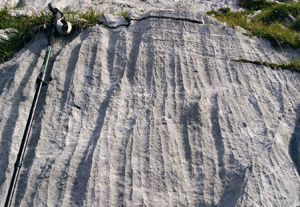
This work deals with dissolutional karren forms. Because karren are characterized by a multitude of shapes (e.g. circular, linear, polygenetic) and spatial scales (from micrometres to tens of metres), karren classification is still debated (Ginés et al. Reference Ginés, Knez, Slabe and Dreybrodt2009). Specifically, we deal with karren of linear forms that are hydrodynamically controlled (instead of fracture controlled, see the classification by Ford & Williams (Reference Ford and Williams2013), table 9.1). These are longitudinal patterns in which the channels originate from the dissolution process driven by the water flow (figure 1). Linear karren patterns are usually grouped in relation to their transverse wavelength (distance between two quasi-parallel channels), which can span different orders of magnitude: from decimetric wandkarren (figure 1a,b) and rinnenkarren, also called runnels, to centimetric rillenkarren (figure 1c,d) and millimetric microrills (figure 1e), also called rillenstein. The pattern classification is not always straightforward. For example, the wandkarren in (b) much recalls the rillenkarren in (d) and probably some authors would call them decantation flutings (Ford & Williams Reference Ford and Williams2013). Furthermore, superimposition of one pattern onto another are very common, such as microrills on rillenkarren, or rillenkarren on rinnenkarren (Ginés et al. Reference Ginés, Knez, Slabe and Dreybrodt2009). There is a reason for these impressive similarities: all these patterns share a common hydrodynamic origin. Although this has always been recognized, to date there is not a comprehensive theory that might explain the regular channelization induced by water (Ginés et al. Reference Ginés, Knez, Slabe and Dreybrodt2009). This theoretical lack is the goal of the present paper.

Figure 1. Linear karren forms of different spatial scales. (a) Wandkarren in limestone, Asturias, Spain. (b) Wandkarren in dolomite, Brenta Dolomites, Italy. (c) Rillenkarren in dolomite, Brenta Dolomites, Italy. (d) Microrills in limestone, Verzino, Calabria, Italy. Credits: I. Benvenuty Cabral for panel (a); Sauro (Reference Sauro2009) for (d).
To this aim, we model a laminar film of undersaturated water that flows down a dissolving inclined rock (see figure 2 for a graphical sketch). The overall chemistry is reduced to the total concentration  $\hat {c}(\hat {\boldsymbol {x}},\hat {t})$ of the solute species within the water film (the hat refers to dimensional quantities). The interactions between the flow field and the concentration field define the temporal evolution of the rock surface. From a mathematical point of view, the dynamic water–rock boundary delineates a Stefan problem for the underlying system of partial differential equations. Notably, in recent years, Stefan problems involving fluid motion have been the subject of several experimental investigations (e.g. Mac Huang, Moore & Ristroph Reference Mac Huang, Moore and Ristroph2015; Wykes et al. Reference Wykes, Mac Huang, Hajjar and Ristroph2018; Cohen et al. Reference Cohen, Berhanu, Derr and du Pont2020; Guérin et al. Reference Guérin, Derr, Du Pont and Berhanu2020) and theoretical analyses (e.g. Moore Reference Moore2017; Morrow et al. Reference Morrow, King, Moroney and McCue2019).

Figure 2. Sketch of the water film flowing on soluble rock. The flat state is characterized by a semi-parabolic profile for the longitudinal velocity  $u_0(\zeta )$ and a two-dimensional concentration field
  $c_0(x,\zeta )$. This is the base state of the transverse (
 $z$-direction) stability analysis.
A modelling novelty of this work regards the dissolution rate, that we here define by directly addressing the local gradient of concentration at the rock–water interface. This is done by spatially solving the advection–diffusion equation for  $\hat {c}(\hat {\boldsymbol {x}},\hat {t})$ and it allows us to avoid the empirical formulations for the dissolution rate that are commonly used in the context of karst pattern formation. These are here briefly summarized for completeness. The simplest formulations link the dissolution–precipitation flux to a hydrodynamic quantity, e.g. the depth-averaged velocity (Goldenfeld et al. Reference Goldenfeld, Chan and Veysey2006; Veysey & Goldenfeld Reference Veysey and Goldenfeld2008) or the water depth (Camporeale Reference Camporeale2015; Bertagni & Camporeale Reference Bertagni and Camporeale2017). Another common approach is to linearly link the dissolution flux to the difference between the saturation concentration and a certain concentration within the water film, e.g. the – uniform – bulk concentration (e.g. Camporeale Reference Camporeale2017) or the concentration at the solid wall (e.g. Claudin et al. Reference Claudin, Durán and Andreotti2017). A more complete formulation for the dissolution flux is the seminal Plummer–Wigley–Parkhurst equation (Plummer, Wigley & Parkhurst Reference Plummer, Wigley and Parkhurst1978), which has been successfully used within the context of karst pattern formation (e.g. Camporeale & Ridolfi Reference Camporeale and Ridolfi2012; Vesipa et al. Reference Vesipa, Camporeale and Ridolfi2015). Although these empirical formulations are sustained by experimental and numerical evidence (Buhmann & Dreybrodt Reference Buhmann and Dreybrodt1985; Hammer et al. Reference Hammer, Dysthe, Lelu, Lund, Meakin and Jamtveit2008; Dreybrodt Reference Dreybrodt2012), they do not address the local gradients of concentration that may develop within the water film.
The paper is structured as follows: in § 2, we formulate the problem of linear karren formation; in § 3, we find the mathematical solutions for the hydrodynamics and the solute concentration in the initial case of a flat rock surface; in § 4, we investigate the linear stability of the flat solution to eventually achieve the dispersion relationship that describes incipient karren formation. The results of the linear stability analysis are reported in § 5 and further discussed, together with some limits of the present model, in § 6. We finally add some concluding remarks in § 7.
2. Formulation of the problem
2.1. Governing equations
A steady water film flowing on a flat surface performs a semi-parabolic velocity profile (figure 2). This is commonly referred to as the Nusselt solution and it can be readily derived from momentum conservation (Nusselt Reference Nusselt1916). Accordingly, the dimensional film thickness and the surface velocity read
 \begin{equation} \hat{h}_0 =\left( \frac{3\nu\hat{q}}{g\sin\theta}\right)^{1/3},\quad \hat{u}_s = \left(\frac{9g\hat{q}^2\sin\theta}{8\nu}\right)^{1/3}, \end{equation}
where  $\nu =10^{-6}$ m
 $^2$ s
 $^{-1}$ is the water kinematic viscosity,
  $g$ is the gravitational acceleration,
  $\theta$ is the angle with the horizontal and
  $\hat {q}=2 \hat {u}_s \hat {h}_0/3$ is the flow rate per unit span. The hat refers to dimensional variables. We use the quantities in (2.1a,b) to scale the governing equations of the problems, which are the Navier–Stokes equations and the advection–diffusion equation for the solute concentration
  $c$ (scaled with its equilibrium value
  $\hat {c}_{{eq}}$, see table 1)
 \begin{gather} \boldsymbol{\nabla} \boldsymbol{\cdot} \boldsymbol{u} = 0, \end{gather}
 \begin{gather}{\textit{Re}} (\boldsymbol{u}\boldsymbol{\cdot}\boldsymbol{\nabla} \boldsymbol{u}+ \boldsymbol{\nabla} p) = \nabla^2 \boldsymbol{u}+\boldsymbol{f}, \end{gather}
 \begin{gather}{\textit{Pe}}\,\boldsymbol{u}\boldsymbol{\cdot}\boldsymbol{\nabla} c = \nabla^2 c, \end{gather}
where  $\boldsymbol {\nabla }=(\partial _x,\partial _y,\partial _z)$,
  $\boldsymbol {u}=(u,v,w)$ is the velocity field (figure 2),
  $p$ is pressure – scaled with
  $\rho \hat {u}_s^2$, with
  $\rho$ the water density – and
  $\boldsymbol {f}=(2,-\delta ,0)$ is the gravity term, with
  $\delta =2\cot {\theta }$. Because of the slow morphological evolution of the rock surface, the quasi-steady approximation (
 $\partial _t=0$) is used in (2.2)–(2.4). The dimensionless numbers appearing in (2.2)–(2.4) are the Reynolds and Péclet numbers, which read
 \begin{equation} {\textit{Re}}=\frac{\hat{u}_s\hat{h}_0}{\nu},\quad {\textit{Pe}}=\frac{\hat{u}_s\hat{h}_0}{D}={\textit{Re}}\,{\textit{Sc}}, \end{equation}
where  $D$ is the molecular diffusivity coefficient. For the solute species considered (table 1), an average value of
  $D\simeq 10^{-9}$ m
 $^2$ s
 $^{-1}$ can be assumed (Ford & Williams Reference Ford and Williams2013). Notice that
  ${\textit {Pe}}$ and
  ${\textit {Re}}$ are linked through the Schmidt number
  ${\textit {Sc}}=\nu /D=10^3$ (
 ${\textit {Pe}}=10^3 {\textit {Re}}$).
Table 1. Dissolution reaction, density and solubility of some representative karst minerals. Solubility is given as the amount of mineral that can be dissolved in water at 25 $^{\circ }$ and
 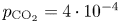 $p_{\text {CO}_2}=4\cdot 10^{-4}$ atm (Dreybrodt Reference Dreybrodt2012; Ford & Williams Reference Ford and Williams2013).

2.2. Hydrodynamic boundary conditions
The boundary conditions are defined on the rock–water interface  $\eta (x,z,t)$ and water–air interface
 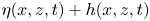 $\eta (x,z,t)+h(x,z,t)$ (figure 2). It is thus convenient to introduce the vertical coordinate
 \begin{equation} \zeta=\frac{y-\eta(x,z,t)}{h(x,z,t)}, \end{equation}
so that the water domain is always defined between  $\zeta =0$ (rock–water interface) and
  $\zeta =1$ (water–air interface). Notice that
  $y$ and
  $\eta$ are measured relative to the position of the initially flat rock surface and they are scaled with
  $\hat {h}_0$.
At the rock–water interface ( $\zeta =0$), the velocity field satisfies the no-slip and impermeability conditions, which are respectively
 \begin{equation} u=w=0,\quad v=0, \end{equation}
where we neglect the influence of the slow dissolution process in the vertical hydrodynamic velocity. At the water–air interface ( $\zeta =1$), the continuity of the stress is ensured by the so-called dynamic conditions
 \begin{equation} \boldsymbol{n}\cdot {\boldsymbol{\mathsf{T}}} \cdot \boldsymbol{n} ={-}{\textit{We}}\,\mathcal{K},\quad \boldsymbol{n}\cdot {\boldsymbol{\mathsf{T}}} \cdot \boldsymbol{t}=0, \end{equation}
where 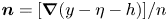 $\boldsymbol {n}=[\boldsymbol {\nabla }(y-\eta -h)]/n$ and
  $\boldsymbol {t}$ are the versors normal and tangent to the free surface (
 $n=\lbrace {1+[\partial _x(h+\eta )]^2+[\partial _z(h+\eta )]^2\rbrace }^{1/2}$ is the versor normalization). Here,
  ${\boldsymbol{\mathsf{T}}}$ is the stress tensor (
 ${\boldsymbol{\mathsf{T}}}_{ij}=p \delta _{ij} - (\partial _{x_i} u_j +\partial _{x_j} u_i)/{\textit {Re}}$). The term
  ${\textit {We}}\,\mathcal {K}$ accounts for the normal stress induced by the surface tension
  $\sigma$, where
  ${\textit {We}}$ is the Weber number and
  $\mathcal {K}$ is the mean curvature of the free surface (e.g. Chang & Demekhin Reference Chang and Demekhin2002)
 \begin{gather} {\textit{We}}=\frac{\sigma}{\rho \hat{h}_0 \hat{u}_s^2}=\frac{{\textit{Ka}}}{{\textit{Re}}^{5/3}\sin{(\theta)}}, \end{gather}
 \begin{gather}\mathcal{K}=\partial_x \left[\frac{\partial_x(h+\eta)}{n}\right]+\partial_z \left[\frac{\partial_z(h+\eta)}{n}\right]. \end{gather}
From (2.9) we notice that  ${\textit {We}}$ is a function of
  ${\textit {Re}}$ and the angle
  $\theta$ through the Kapitza number
 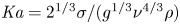 ${\textit {Ka}}=2^{1/3} \sigma /(g^{1/3} \nu ^{4/3} \rho )$;
  ${\textit {Ka}}$ only depends on the water properties and is thus constant for our purposes.
The temporal evolution of the free surface is described by the kinematic condition in  $\zeta =1$
 \begin{equation} \partial_t h = \boldsymbol{u}\cdot\boldsymbol{n}=v-u (h+\eta)_x - w (h+\eta)_z, \end{equation}
where, as in (2.7a,b), we neglected the influence of  $\eta _t$ in the hydrodynamics. Equation (2.11) ensures the water mass conservation and will be later used as the first solvability equation.
2.3. Concentration boundary conditions
Differently from the hydrodynamic quantities, the concentration  $c$ has also a longitudinal dependence due to the downstream solute accumulation within the water film (see figure 2). Basically, this makes the concentration field a three-dimensional problem. In fact,
  $c$ depends on
  $x$ because of the downstream solute accumulation, on
  $y$ due to the normal-to-wall effect of the dissolution occurring at the rock–water interface and on
  $z$ because of the transverse nature of linear karren forms.
Upstream, as the water film is generally produced by rain or snow melt, it might be considered free of solute
 \begin{equation} c\vert_{x=0}=0. \end{equation}
 With the dissolution of the rock surface, solute molecules are dissociated from the solid through chemical reactions and then transported into the film bulk by diffusion. In general, the slowest between these two processes (surface reaction and transport by diffusion) controls the dissolution kinetics of a karst rock. Very soluble minerals, such as salt, have a rapid dissolution reaction and thus the kinetics is always diffusion controlled (Ford & Williams Reference Ford and Williams2013). For relatively less soluble minerals, such as gypsum or calcite, numerous studies have demonstrated that in very undersaturated waters, such as those commonly found in exposed karst environments, a diffusion-controlled dissolution kinetics prevails (see the review on dissolution kinetics by Morse & Arvidson (Reference Morse and Arvidson2002), and references therein). As equilibrium is approached, there is a transition region to a surface-controlled dissolution kinetics. Moreover, for calcite, which dissolves in water enriched with CO $_2$, the slow uptake of CO
 $_2$ from the atmosphere may also become a limiting factor as equilibrium is approached (Buhmann & Dreybrodt Reference Buhmann and Dreybrodt1985; Kaufmann & Dreybrodt Reference Kaufmann and Dreybrodt2007). Notice that CO
 $_2$-conversion does not influence salt and gypsum dissolution as they directly dissociate in pure water (table 1).
Since we wish to model incipient karren formation and linear karren forms have been observed to develop upstream first, i.e. where the water is very undersaturated (Glew & Ford Reference Glew and Ford1980; Ginés et al. Reference Ginés, Knez, Slabe and Dreybrodt2009; Slabe, Hada & Knez Reference Slabe, Hada and Knez2016), we consider a dissolution kinetics that is diffusion controlled. This implies that surface reactions are fast compared to diffusion and that the solute accumulates in a very thin diffusion boundary layer at the solid–liquid interface that is nearly saturated (e.g. Ford & Williams Reference Ford and Williams2013). By also imposing no flux of solute between water and air, the vertical boundary conditions eventually read
 \begin{equation} \partial_\zeta c\vert_{\zeta=1} = 0,\quad c\vert_{\zeta=0}=1. \end{equation}
 The morphological evolution of the rock surface is thus regulated by the flux of solute that moves into the bulk of the water film through diffusion, i.e. 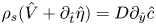 $\rho _s (\hat {V}+\partial _{\hat {t}}\hat {\eta })= D \partial _{\hat {y}} \hat {c}$, where
  $\rho _s$ is the rock density and
  $\hat {V}$ is the dissolution rate induced by the uniform hydrodynamic flow (
 $\hat {V}<0$). In dimensionless form, the same equation reads
 \begin{equation} \gamma\,{\textit{Pe}}\,h(V+\partial_t \eta) = \partial_\zeta c, \end{equation}
where  $\gamma =\rho _s/\hat {c}_{eq}\gg 1$ is related to the mineral considered (table 1). Equation (2.14) will be used as the second solvability equation.
3. Flat-rock solution
We here find the solution to the problem (2.2)–(2.14) for an initially flat rock surface, i.e.  $\eta _0=\partial _z=0$ and
  $h_0=1$, where the subscript
  $0$ denotes the absence of karren patterns.
3.1. Hydrodynamics
The Navier–Stokes equations (2.2) and (2.3) reduce to
 \begin{equation} u_0''={-}2,\quad p_0'={-}\delta/{\textit{Re}}, \end{equation}
with boundary conditions
 \begin{equation} u_0\vert_{\zeta=0}=0,\quad u_0'\vert_{\zeta=1}=0,\quad p_0\vert_{\zeta=1}=0, \end{equation}
where  $'$ denotes differentiation in
  $\zeta$. The solutions are the Nusselt semi-parabolic profile for the longitudinal velocity and the hydrostatic pressure profile
 \begin{equation} u_0=(2-\zeta)\zeta,\quad v_0=w_0=0,\quad p_0=\frac{\delta}{{\textit{Re}}} (1-\zeta). \end{equation}
3.2. Concentration
The advection–diffusion equation (2.4) reduces to
 \begin{equation} {\textit{Pe}}\,u_0(\zeta)\partial_x c_0 = c_0'', \end{equation}
where the longitudinal diffusion has been neglected since its effect is smaller than that of longitudinal advection. The initial and boundary conditions (2.12) and (2.13a,b) read
 \begin{equation} c_0\vert_{x=0}=0,\quad c_0\vert_{\zeta=0}=1,\quad c_0'\vert_{\zeta=1}=0. \end{equation}
Equation (3.4) highlights the coupling between the concentration field  $c_0$ and the velocity profile
  $u_0(\zeta )$, as well as the
  $x$-dependency of the concentration distribution due to the downstream solute accumulation. The solution to this problem is resumed in Polyanin et al. (Reference Polyanin, Kutepov, Kazenin and Vyazmin2001, pp. 130–132) and it is here more extensively reported. For
  $x\ge 0$, we seek the solution in the form of the series (Davis Reference Davis1973)
 \begin{equation} c_0=1-\sum_{m=0}^{\infty} A_m F_m(x)G_m(\zeta), \end{equation}
where 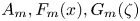 $A_m, F_m(x),G_m(\zeta )$ are unknown functions that must be determined. Substituting the expansion (3.6) into (3.4) and then separating the variables, we obtain
 \begin{gather} \partial_x F_m(x)+\frac{\alpha_m^2}{{\textit{Pe}}}F_m(x)=0, \end{gather}
 \begin{gather}G_m''(\zeta)+\alpha^2_m u_0(\zeta) G_m(\zeta)=0. \end{gather}
The solution to the  $x$-problem (3.7) is readily given by
 \begin{equation} F_m(x)=\exp{\left(-\alpha^2_m\frac{x}{{\textit{Pe}}}\right)}. \end{equation}
Instead, (3.8) defines a Sturm–Liouville problem, whose boundary conditions, that are obtained after replacement of (3.6) into the second and third equations in (3.5a–c), are
 \begin{equation} G_m\vert_{\zeta=0}=0,\quad G_m'\vert_{\zeta=1}=0. \end{equation}
The solution of the Sturm–Liouville problem for the eigenfunctions  $G_m$ (up to a constant factor) is
 \begin{equation} G_m(\zeta)=\exp{\left[-\frac{\alpha_m}{2}(1-\zeta)^2\right]} {\Phi}\left(\frac{1}{4}-\frac{\alpha_m}{4},\frac{1}{2};\alpha_m(1-\zeta)^2\right), \end{equation}
where  ${\Phi }(\cdot ,\cdot;\cdot )$ is the degenerate hypergeometric function (Abramowitz, Stegun & Romer Reference Abramowitz, Stegun and Romer1988). Substituting (3.11) into the first of the boundary conditions (3.10a,b) provides the transcendental equation for the eigenvalues
  $\alpha _m>0$
 \begin{equation} {\Phi}\left(\frac{1}{4}-\frac{\alpha_m}{4},\frac{1}{2};\alpha_m\right)=0. \end{equation}
For the definition of the coefficients  $A_m$, the first step is to substitute the series (3.6) into the first equation in (3.5a–c), which yields
 \begin{equation} \sum_{m=0}^{\infty} A_m G_m(\zeta)=1. \end{equation}
Multiplying (3.13) by  $u_0G_n$, with
  $n\neq m$, then integrating between
  $\zeta =0$ and
  $\zeta =1$, and using the orthogonality condition
 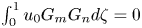 $\int _0^1 u_0 G_m G_n d\zeta =0$, one obtains
 \begin{equation} A_m=\frac{\int_0^1 u_0 G_m(\zeta)\,\textrm{d}\zeta}{\int_0^1 u_0 G_m(\zeta)^2\,\textrm{d}\zeta}. \end{equation}
Notably, instead of solving numerically (3.12) and (3.14), it is possible to evaluate the constants  $A_m$ and
  $\alpha _m$ with the approximated relationships (Polyanin & Nazaikinskii Reference Polyanin and Nazaikinskii2015)
 \begin{gather} \alpha_m=4m+1.68 \quad (m=0,1,2\cdots), \end{gather}
 \begin{gather}A_0=1.2,\quad A_m=({-}1)^m 2.27\alpha_m^{{-}7/6} \quad (m=1,2,3\cdots), \end{gather}
whose maximum error is less than 0.2 %. It is also worth mentioning that, for  $x/{\textit {Pe}} \rightarrow 0$, an easier asymptotic solution for
  $c_0$ can be obtained (Polyanin et al. Reference Polyanin, Kutepov, Kazenin and Vyazmin2001)
 \begin{equation} c_0={\Gamma}\left(\frac{1}{3},\frac{2 \zeta ^3}{9 X}\right)/{\Gamma} \left(\frac{1}{3}\right) \quad \mbox{for}\ x/{\textit{Pe}}=X\rightarrow 0, \end{equation}
where  $\Gamma (\cdot )$ and
  ${\varGamma }(\cdot ,\cdot )$ are the complete and incomplete gamma functions (Abramowitz et al. Reference Abramowitz, Stegun and Romer1988);
  $X=x/{\textit {Pe}}$ is a convenient scaling that maps the dissolution domain of the problem between
  $X=0$, where the water is free of solute, and
  $X=1$, where the water film is basically saturated. In fact, some easy algebra shows that the time scale
  $\hat {\tau }$ needed by water to go from
  $X=0$ to
  $X=1$ is
  $\hat {\tau }\sim \hat {h}_0^2/D$, i.e. equivalent to the time scale required by diffusion to involve the full water depth.
The spatial trends of the exact solution (3.6) and the asymptotic solution (3.17) for  $c_0$ are shown in figure 3.

Figure 3. Vertical profiles of  $c_0$ at different
  $X$ (log scale). The solid red lines refer to the exact solution (3.6). The dotted-black lines refer to the asymptotic solution (3.17), which is shown to be valid up to
  $X\sim 0.1$. The coloured areas evidence the saturation ratio of water in the solute.
3.3. Dissolution
The dissolution rate  $V$ can be evaluated by combining the evolution equation for the rock surface (2.14) and the solution for
  $c_0$
$c_0$
 \begin{equation} V=\frac{1}{\gamma\,{\textit{Pe}}}c_0' \vert_{\zeta=0}. \end{equation}
It is also convenient to define the saturation ratio  $s$ as
 \begin{equation} s=\int_0^1 c_0\,\textrm{d}\zeta, \end{equation}
where  $s=0$ indicates pure water and
  $s=1$ corresponds to saturated water (ion pairing is neglected). Because the concentration has been scaled with its saturation value,
  $s$ is also equivalent to the dimensionless depth-averaged concentration. A graphical evidence of the saturation ratio of the water film is given by the light red areas in the panels of figure 3.
The trend  $V=V(X)$, obtained after replacing (3.6) in (3.18), is reported in figure 4(a). Notice that the quantity
  $\gamma {\textit {Pe}}\,\lvert V \rvert$ is independent of the rock type and the film hydrodynamics. The dissolution rate decreases with
  $X$ as the water loses chemical aggressivity by increasing its saturation ratio
  $s$ (right
  $y$-axis). Because clear water enhances dissolution, half-saturation (
 $s=0.5$) is reached in the upstream part of the flow (
 $X\sim 0.2$) and the rate of solute accumulation progressively decreases downstream. Although at
  $X=1$ the flow is not completely saturated (coloured area in figure 3d) at those levels of saturation – and even before (
 $s>0.9$) – dissolution is known to drop drastically because of the inhibitory action of other chemical species in the rock texture (Kaufmann & Dreybrodt Reference Kaufmann and Dreybrodt2007; Ford & Williams Reference Ford and Williams2013).

Figure 4. Dissolution of an initially flat rock. (a) Longitudinal trends of the scaled dissolution rate  $\gamma {\textit {Pe}} \lvert V\rvert$ (blue) and the saturation ratio
  $s$ (red); (b)
  $\gamma {\textit {Pe}} \lvert V\rvert$ versus
  $s$, from the previous panel, highlighting a nonlinear relationship with a change of dissolution rate around
  $s\sim 0.3$.
Between the saturation ratio  $s$ and the dissolution rate, there is a nonlinear relationship (figure 4b). This nonlinearity, which here arises thanks to the spatially dependent solution for the concentration, highlights the limits of the common assumption of a diffusive flux linearly related to the saturation ratio, i.e.
  $V\propto (s-1)$. Indeed, the dissolution of the rock surface is better specified by the local gradient of concentration at the rock surface (
 $c_0'\vert _{\zeta =0}$), rather than by the average concentration gradient along the film thickness (
 $s-1$ dimensionally scales with
  $(\hat {c}-\hat {c}_{{eq}})/\hat {h}_0$). Furthermore, it is remarkable to notice that the trend in figure 4(b) is qualitatively similar to experimental evidence for calcite dissolution (Buhmann & Dreybrodt Reference Buhmann and Dreybrodt1985; Kaufmann & Dreybrodt Reference Kaufmann and Dreybrodt2007), even though we here consider a simplified dissolution kinetics that is controlled just by diffusion. Kaufmann & Dreybrodt (Reference Kaufmann and Dreybrodt2007) have in fact shown that two quasi-linear regimes (for
  $s<0.3$ and
  $s>0.3$) can be considered in the dissolution rate of calcite. These regimes have linear coefficients separated by an order of magnitude and they have been qualitatively plotted with dashed lines in figure 4(b).
4. Linear stability analysis
We here evaluate the stability of the flat-rock solution reported in the previous section to a small transverse perturbation written in normal modes
 \begin{align} (\boldsymbol{u},p,c,h,\eta) &= (\boldsymbol{u}_0(\zeta),p_0(\zeta),c_0(\zeta,X),1,0) \nonumber\\ &\quad +\varepsilon(\boldsymbol{u}_1(\zeta),p_1(\zeta),c_1(\zeta,X),h_1,\eta_1)\exp({\omega t + \mathrm{i} k z}), \end{align}
where  $\varepsilon$ is an infinitesimal parameter,
  $k$ is the transverse wavenumber and
  $\omega$ is the growth rate. Due to the transverse invariance of the problem,
  $\omega$ is a real number, i.e. there is no angular phase. When
  $\omega >0$, the base state is unstable and the perturbation grows in time to eventually form periodic longitudinal patterns.
The ansatz (4.1) follows the assumption of longitudinal invariance ( $\partial _x=0$) just for the hydrodynamic quantity (
 $\boldsymbol {u},p,h$) and not for the concentration field, which has a longitudinal structure given by the solute accumulation within the water film. The variable
  $X$ defines the transverse section wherein the linear stability analysis is performed.
4.1. Hydrodynamics
Since the hydrodynamic problem is longitudinally invariant, the continuity equation (2.2) at the linear order ( $\varepsilon$) imposes
 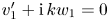 $v_1'+\mathrm {i}\,kw_1=0$. Therefore, we can introduce the scalar streamfunction
  $\varphi$, such that
 \begin{equation} v_1={-}\mathrm{i} k \varphi,\quad w_1=\varphi'. \end{equation}
After some algebraic manipulations, the Navier–Stokes equations (2.2)-(2.3) are reduced to the Orr–Sommerfeld equation for a domain longitudinally invariant (e.g. Chang & Demekhin Reference Chang and Demekhin2002; Kalliadasis et al. Reference Kalliadasis, Ruyer-Quil, Scheid and Velarde2011)
 \begin{equation} \varphi^{iv}-2 k^2 \varphi''+k^4 \varphi =0, \end{equation}
with boundary conditions
 \begin{gather} \varphi'=\varphi=0 \quad \text{in}\ \zeta=0, \end{gather}
 \begin{gather}\varphi ''+k^2 \varphi=\varphi ^{(3)}-3 k^2 \varphi '-\mathrm{i} k (\eta_1+h_1) (k^2 {\textit{Re}}\,{\textit{We}}+\delta)=0\quad \text{in}\ \zeta=1. \end{gather}
We recall that (4.4) are the no-slip and impermeability conditions at the rock–water interface (corresponding to (2.7a,b)), while (4.5) are the linearized dynamic conditions at the water–air interface, (2.8a,b). The advantage of the Orr–Sommerfeld approach is that the transverse hydrodynamic problem is reduced to the biharmonic equation (4.3), the solution thereof is
 \begin{equation} \varphi=\mathrm{i}\,(\delta+k^2 {\textit{Re}} {\textit{We}})(\eta_1+h_1)f(\zeta), \end{equation}
where
 \begin{equation} f(\zeta)=\frac{(k \zeta \coth (k \zeta )-1) (k \sinh{k}+\cosh{k})-k^2 \zeta \cosh{k}}{k (2 k^2+\cosh (2 k)+1)}\sinh{(k \zeta)}. \end{equation}
Combining (4.2a,b) and (4.6) readily provides the solution for  $v_1$ and
  $w_1$ (where the latter can be shown to be much larger than the former). Because of the longitudinal invariance of the linear problem,
  $u_1$ is not explicitly related to
  $\varphi$. Thus, for its evaluation, we directly address the conservation of longitudinal momentum (2.3), which at order
  $\varepsilon$ reads
 \begin{equation} u_1''-k^2 u_1={-}k^2 u_0'(\eta_1+\zeta h_1)+{\textit{Re}}\,u_0'v_1 +2 u_0'' h_1, \end{equation}
with boundary conditions
 \begin{equation} u_1\vert_{\zeta=0}=0,\quad u_1'\vert_{\zeta=1}=0. \end{equation}
The terms in the left side of (4.8) are the vertical and transverse diffusion of momentum, respectively. The terms in the right side arise from advection ( ${\textit {Re}}\,u_0'v_1$) and the change of the vertical coordinate (from
  $y$ to
  $\zeta$, see (2.6)).
By solving the (4.8) through the method of variation of parameters (e.g. Bender & Orszag Reference Bender and Orszag2013), we eventually obtain
 \begin{equation} u_1=2\textrm{sech}{k}\left[(\eta_1+h_1) \sinh (k \zeta )/k - \eta_1 \cosh (k -k \zeta )\right]+2(1-\zeta ) (\eta_1+\zeta h_1), \end{equation}
where the contribution of  $v_1$ in (4.10) has been neglected as it would considerably complicate the solution without any perceptible numerical change.
4.2. Concentration
At  $\mathcal {O}(\varepsilon )$, the linearized advection–diffusion equation (2.4) reads
 \begin{equation} c_1''-k^2 c_1 + \varUpsilon(\zeta,X) =u_0(\zeta)\partial_X c_1 \end{equation}
where  $\varUpsilon$ is the inhomogeneous term
 \begin{equation} \varUpsilon(\zeta,X)=k^2 c_0' (\eta_1+\zeta h_1)-{\textit{Pe}}\,c_0' v_1-2 h_1 c_0'' -u_1 \partial_X c_0, \end{equation}
and the initial and boundary conditions (2.12) and (2.13a,b) are
 \begin{equation} c_1\vert_{X=0} =0,\quad c_1\vert_{\zeta=0}=0,\quad c_1'\vert_{\zeta=1}=0. \end{equation}
The solution to the problem (4.11)–(4.13a–c) is (Polyanin & Nazaikinskii Reference Polyanin and Nazaikinskii2015)
 \begin{equation} c_1=\int_0^X\int_0^1 \varUpsilon(\zeta_m,X_m)\mathcal{G}(\zeta,\zeta_m,X-X_m)\,\textrm{d}\zeta_m \,\textrm{d} X, \end{equation}
where  $\zeta _m$ and
  $X_m$ are dummy variables, and
  $\mathcal {G}$ is the modified Green's function
 \begin{equation} \mathcal{G}(\zeta,\zeta_m,X)= \sum_{m=0}^{\infty} \frac{\mathcal{H}_m(\zeta)\mathcal{H}_m(\zeta_m)}{\|\mathcal{H}_m^2\|}\mathcal{F}_m(X),\quad \|\mathcal{H}_m^2\|=\int_0^1 u_0 \mathcal{H}_m^2 \,\textrm{d}\zeta. \end{equation}
Here,  $\mathcal {H}_m(\zeta )$ and
  $\mathcal {F}_m(X)$ are the solutions associated with the homogeneous part of (4.11). They can be obtained, after separation of variables, following the procedure used to solve the base-state problem (3.4)–(3.5a–c) for
  $c_0$. The
  $X$-problem leads to
 \begin{equation} \mathcal{F}_m(X)=\exp{\left(-\lambda^2_mX\right)}. \end{equation}
The  $\zeta$-problem defines the Sturm–Liouville problem
 \begin{gather} \mathcal{H}_m''(\zeta)+\left(\lambda^2_m u_0(\zeta)-k^2\right) \mathcal{H}_m(\zeta)=0, \end{gather}
 \begin{gather}\mathcal{H}_m\vert_{\zeta=0}=0,\quad \mathcal{H}_m'\vert_{\zeta=1}=0, \end{gather}
whose solution for the eigenfunctions  $\mathcal {H}_m$ (up to a constant factor) is
 \begin{equation} \mathcal{H}_m(\zeta)=\exp{\left[-\frac{\lambda_m}{2}(1-\zeta)^2\right]} {\Phi}\left(\frac{k^2+\lambda_m-\lambda_m^2}{4\lambda_m},\frac{1}{2};\lambda_m(1-\zeta)^2\right). \end{equation}
Substituting (4.19) into the first of the boundary conditions (4.18a,b) provides the transcendental equation for the eigenvalues  $\lambda _m>0$
 \begin{equation} {\Phi}\left(\frac{k^2+\lambda_m-\lambda_m^2}{4\lambda_m},\frac{1}{2};\lambda_m\right)=0, \end{equation}
which highlights how the eigenvalues  $\lambda _m$ are functions of the wavenumber
  $k$.
$k$.
We recall that, to evaluate the rock dissolution, we only need the concentration gradient at the rock–water interface (see (2.14)). Using the solution (4.14) and separating the terms related to  $h_1$ and
  $\eta _1$, the gradient at the rock–water interface reads
 \begin{equation} c_1'\vert_{\zeta=0}=\mathcal{I}_{h_1} h_1+\mathcal{I}_{\eta_1}\eta_1, \end{equation}
where the expressions for the integral terms  $\mathcal {I}_{h_1}$ and
  $\mathcal {I}_{\eta _1}$ are reported in appendix A.
4.3. Dispersion relationship
At this point, (2.11) and (2.14) are adopted as solvability equations. These describe the temporal evolution of the rock–water and water–air interfaces and, at order  $\varepsilon$, they read
 \begin{gather} \omega h_1 = \mathrm{i} k \varphi \vert_{\zeta=1} \end{gather}
 \begin{gather}\omega \eta_1 = \frac{1}{\gamma {\textit{Pe}}} c_1'\vert_{\zeta=0}-h_1V. \end{gather}
Substituting the solutions for the streamfunction (4.6) and the concentration gradient (4.21), we obtain the linear system
 \begin{equation} \omega \left(\begin{array}{c} h_1 \\ \eta_1 \end{array}\right) = \left(\begin{array}{cc} a_1 & a_2\\ a_3 & a_4 \end{array}\right)\cdot\left(\begin{array}{c} h_1 \\ \eta_1 \end{array}\right), \end{equation}
where
 \begin{gather} a_1=a_2=\frac{(k^2 {\textit{Re}}\,{\textit{We}}+\delta) (k-\cosh{k} \sinh{k})}{k (2 k^2+\cosh (2 k)+1)}, \end{gather}
 \begin{gather}a_3=\frac{\mathcal{I}_{h_1}}{\gamma\,{\textit{Pe}}}-V,\quad a_4=\frac{\mathcal{I}_{\eta_1}}{\gamma\,{\textit{Pe}}}. \end{gather}
The system (4.24) admits two non-trivial solutions for the eigenvalues
 \begin{equation} \omega_{\eta,h}=\frac{(a_1+a_4)\pm\sqrt{(a_1+a_4)^2-4a_1(a_4-a_3)}}{2}, \end{equation}
which we discriminate with the subscripts  $h$ and
  $\eta$, as it will be shown in the following that the former is related to the free surface and the latter to the rock surface.
By assuming the rigid lid approximation (RLA) on the free surface i.e. imposing  $h_t=0$ in the kinematic condition (2.11), the first equation in the system (4.24) reduces to
  $h_1=-\eta _1$. In this case, the problem provides just one eigenvalue
 \begin{equation} \omega_{{RLA}}=V+\frac{(\mathcal{I}_{\eta_1}-\mathcal{I}_{h_1})}{\gamma{\textit{Pe}}}. \end{equation}
By substituting  $h_1=-\eta _1$ into the streamfunction (4.6), it is also evident that the RLA induces zero spanwise and vertical velocities, i.e.
  $v_1=w_1=0$. The existence of a secondary flow in the cross-sectional plane is in fact strictly related to the free surface dynamics. Instead, the streamwise velocity perturbation (4.10) is still non-null as it is triggered by the bottom perturbation. In the next section, we will discuss on the validity and the convenience of this approximate solution in the context of karren formation.
5. Results
The dispersion relationship (4.27) links the two growth rates,  $\omega _h$ and
  $\omega _\eta$, to the transverse wavenumber
  $k$ and the control parameters that embody the physics of the problem. In particular,
  $\omega _h$ is associated with development of hydrodynamic waves on the free surface (rivulets) and
  $\omega _\eta$ is related to the growth of patterns on the rock surface (karren). Hence, our focus is on the morphological eigenvalue
  $\omega _\eta$. The control parameters are: the Reynolds number
  ${\textit {Re}}$, which is related to the flow rate; the longitudinal coordinate
  $X$, which is a proxy for the saturation ratio
  $s$ (figure 4a); the angle of the rock inclination
  $\theta$; the parameter
  $\gamma$, which is associated with the mineral type (table 1).
Summarizing, when  $\omega _\eta >0$, the perturbation grows in time (instability) generating the karren pattern. On the contrary,
  $\omega _\eta <0$ indicates that the perturbation decays in time (stability) restoring the base-state solution. The condition
  $\omega _\eta =0$ discriminates between stable and unstable domains, and its trend in the parameter space evidences the neutral stability curve. Figure 5(a) shows that the rock–water interface is unstable to a band of wavenumbers between 0 and a cutoff value
  $k_c$ for any
  ${\textit {Re}}$, i.e. there is no critical Reynolds number for karren formation. The cutoff wavenumber
  $k_c$ is independent of
  ${\textit {Re}}$ (vertical line in figure 5a) meaning that, dimensionally speaking,
  $k_c$ scales with the flow depth.

Figure 5. Karren instability. (a) Contour plot of the least stable growth rate  $\omega _\eta$ in the
  $\{k,{\textit {Re}}\}$ plane (
 $X=0.05$,
  $\theta ={\rm \pi} /4$, calcite). The neutral stability curve is reported with a black solid line. The cutoff
  $k_c$ and fastest growing
  $k_m$ wavenumbers are highlighted. The numbers on the contours are the values of
  $\omega _\eta$. (b) Growth rates versus the wavenumber
  $k$ (
$k$ ( $X=0.01$,
 ${\textit {Re}}=1$).
  $\omega _h$ and
  $\omega _\eta$ (red solid lines) are the hydrodynamic-stable and morphological-unstable eigenvalues, respectively, from (4.27). The value of
  ${\rm \Delta} k$ is the interval of unstable wavenumbers with growth rate very close to the one of
  $k_m$ (see § 6.2);
  $\omega _{{RLA}}$ (dotted light line) is the morphological growth rate obtained in the RLA, from (4.28). (c) Role of mass (
 $\partial _z^2 c$) and momentum (
 $\partial _z^2 u$) diffusion on
  $\omega _\eta$. The light-blue line is
  $\omega _\eta$ evaluated including
  $v_1$ in the solution for
  $u_1$ and
  $c_1$ (it is indistinguishable from the red line for
  $k>10^{-4}$).
For a fixed value of  ${\textit {Re}}$, the behaviour of the morphological eigenvalue
  $\omega _\eta$ versus the wavenumber is reported in figure 5(b). The maximum of the growth rate, i.e. the fastest growing mode, is indicated with
  $k_m$. As commonly done in linear stability analyses (Cross & Hohenberg Reference Cross and Hohenberg1993), we assume
  $k_m$ to be pattern wavenumber. Yet, as karren instability shows a band of wavenumbers (indicated with
  ${\rm \Delta} k$) with growth rates very close to that of
  $k_m$, we will later add some considerations on the validity of this assumption (§ 6.2).
Figure 5(b) also reports the trends of the hydrodynamic eigenvalue  $\omega _h$ and the approximated morphological eigenvalue
  $\omega _{{RLA}}$, obtained in the RLA. The hydrodynamic eigenvalue is always stable (
 $\omega _h<0$) for the angles of karren formation (
 $\theta <{\rm \pi} /2$) due to the stabilizing effects of gravity and surface tension, which prevent any transverse wave (rivulet) forming. It is interesting to notice that gravity becomes instead destabilizing in overhanging conditions (
 $\theta >{\rm \pi} /2$), creating water rivulets that initiate longitudinal precipitation patterns (Camporeale Reference Camporeale2015; Bertagni & Camporeale Reference Bertagni and Camporeale2017).
The morphological eigenvalue  $\omega _{{RLA}}$ well reproduces the overall system dynamics when the free surface responds very quickly to the rock evolution (
 $\lvert \omega _h\rvert \gg \omega _\eta$) and thus it can be considered flat (
 $\partial _t{h}=0$). This is indeed the case for the wavenumbers involved in karren formation. In fact,
  $\omega _{{RLA}}=\omega _\eta$ for the fastest growing mode
  $k_m$. However,
  $\omega _{{RLA}}$ loses reliability for perturbations with wavelengths so long that hydrodynamic and morphological time scales are comparable (
 $\lvert \omega _h\rvert \sim \omega _\eta$). Although these very long wavelengths are outside the range of karren patterns, to neglect them by freezing the free-surface dynamics prevents us from mathematically obtaining the fastest growing mode
  $k_m$. We also notice that the RLA introduces an error in the mass conservation (
 $\omega _{{RLA}}\neq 0$ for
  $k=0$). In fact, in the particular case
  $k=0$, which corresponds to a spatially uniform perturbation of the base state – the so-called Goldstone mode (e.g. Kalliadasis et al. Reference Kalliadasis, Ruyer-Quil, Scheid and Velarde2011) – the base state is vertically and uniformly shifting, and the water depth must preserve its length to assure mass conservation. So the correct solution should be
  $h_1=0$ instead of
  $h_1=-\eta _1$ as imposed by the RLA. Yet, the latter approximation may be adopted, for example, for a quicker evaluation of the time scale of the instability as
 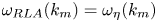 $\omega _{{RLA}}(k_m)=\omega _\eta (k_m)$.
In figure 5(c), we show that the stabilization of the high wavenumbers (short wavelengths) is induced by a coupling of the transverse diffusion of longitudinal momentum –  $\partial _z^2 u$ in (2.3) – and solute –
  $\partial _z^2 c$ in (2.4). In particular, the dashed green and orange lines are the eigenvalues obtained without the transverse diffusion of solute and momentum, respectively. Instead, the dash-dot line is the eigenvalue without both diffusion processes (
 $\partial _z^2 c$ and
  $\partial _z^2 u$) that highlights how diffusion in needed for a cutoff mode
  $k_c$ and a fastest growing mode
  $k_m$ to arise.
Furthermore, we may notice by observing the dotted line in figure 5(c) that including the vertical velocity  $v_1$ in the solutions of
  $u_1$ (4.10) and
  $c_1$ (4.14) complicates their analytical expressions (which are not reported here) and causes numerical issues when solving the integrals in (4.21) for small
  $k$, but overall it does not affect karren instability (the dotted and solid lines in figure 5(c) are indistinguishable for
  $k>10^{-4}$).
The influence of the other control parameters ( $X$,
$X$,  $\theta$,
  $\gamma$) on the morphological growth rate
  $\omega _\eta$ is shown in figure 6. The contour plot 6(a) in the plane
  $\{k,X\}$ shows two maxima: one very close to the water inlet (
 $X<10^{-2}$) and one further downstream (
 $X\sim 0.5$). This suggests that the pattern may first develop at two different longitudinal locations. Yet, a fully nonlinear analysis could probably reveal some influence of the upstream part of the growing pattern on the downstream dissolution process. The wavenumber
  $k_m$ (dashed line) is not strongly affected by
  $X$.
$X$.

Figure 6. Influences of  $X$, the rock angle
  $\theta$ and the rock mineral on karren instability for a fixed water flow (
 ${\textit {Re}}=1$). (a) Contour plot of the morphological growth rate
  $\omega _\eta$ in the
  $\{k,X\}$ plane (calcite,
  $\theta ={\rm \pi} /4$). The dashed line marks the fastest growing modes. (b) Morphological growth rate
  $\omega _\eta$ versus
  $k$ for several angles
  $\theta$ (
 $\theta ={\rm \pi} /8, {\rm \pi}/4, 3{\rm \pi} /8, {\rm \pi}/2$, calcite and
  $X=0.01$). The stars mark the fastest growing modes. (c) Morphological growth rate
  $\omega _\eta$ versus
  $k$ for several mineral types (
 $\theta ={\rm \pi} /4$,
  $X=0.01$ and
  $\gamma$ from table 1 for the three minerals.).
For a fixed  ${\textit {Re}}$, the angle
  $\theta$ seems to have very little influence on karren instability, besides a stabilizing effect at long wavelengths (figure 6b). In contrast, the solubility of the mineral is shown to boost the instability (figure 6c), so that the time scale of karren formation with respect to the rock type is
  $\textrm {salt}<\textrm {gypsum}<\textrm {limestone}$, in agreement with field observations (Mottershead & Lucas Reference Mottershead and Lucas2001).
6. Discussion
The positive feedback responsible for karren instability can be understood by observing the longitudinal velocity and concentration fields in perturbed conditions (figure 7). In correspondence with the rock trough, the deeper and faster flow (a) more efficiently transports away the solute concentration. This leads to a lower concentration of solute in the water (b,c) and to an increased dissolution, which further deepens the rock trough. The opposite happens on the rock crest, where dissolution is dampened. This positive feedback mechanism generates linear karren forms. The spatial scale of the instability is influenced by the transverse diffusive processes of longitudinal velocity and solute (figure 5c). In figure 7, we may also notice that the free surface is basically flat, further indicating the validity of the RLA for the wavenumber of karren formation ( $k\sim k_m$).

Figure 7. Instability mechanism. Transverse sections (vertically exaggerated) showing the response of the longitudinal velocity  $u_1$ (a) and the concentration
  $c_1$ (b,c) to a small perturbation of the rock surface (calcite,
 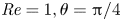 ${\textit {Re}}=1, \theta ={\rm \pi} /4$,
 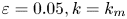 $\varepsilon =0.05, k=k_m$,
  $X=0.01$ for panel (b) and
  $X=0.1$ for (c)). Here,
  $c_1$ varies along
  $X$ inheriting the longitudinal trend of the concentration
  $c_0$ at the base state (see figure 3).
6.1. Dimensional features
The fastest growing mode  $k_m$ of the linear stability analysis provides the dimensional wavelength
  $\hat {L}=2{\rm \pi} /k_m$ and an indication of the time scale of the instability
 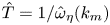 $\hat {T}=1/\hat {\omega }_{\eta }(k_m)$. Figure 8 explores the dependence of these dimensional quantities on the control parameters
  ${\textit {Re}}$ and
  $X$.
$X$.

Figure 8. Contour plots in the  $\{X,{\textit {Re}}\}$ plane for the dimensional wavelength
  $\hat {L}$ (a) and time scale of the instability
  $\hat {T}$ (b) from the linear stability analysis (calcite and
  $\theta ={\rm \pi} /4$). The upper
  $x$-axis reports the saturation ratio
  $s$.
$s$.
The water flow rate ( ${\textit {Re}}$) is shown to play a crucial role in karren formation. In fact,
  $\hat {L}$ increases with the Reynolds number, spanning several orders of magnitude: from millimetric to decimetric values (figure 8a). This result supports the so far speculative idea that it is the flow rate that discriminates the linear karren type: very thin water films (
 ${\textit {Re}}\sim 10^{-3}$) originating from dew or sea spray give rise to millimetric microrills; thicker water films (
 ${\textit {Re}}\sim 10^{-1}-1$) produced by rainwater are responsible for the formation of centimetric rillenkarren; and decimetric wandkarren are formed by high water flows (
 ${\textit {Re}}>10$), which develop downstream of a basin where rain or snow-melt water accumulates (e.g. on a hill slope). Even
  $\hat {T}$ is highly dependent on
  ${\textit {Re}}$, ranging from tens of minutes to weeks (figure 8b). These time scales seem pretty short. Indeed, they are closer to experimental evidence of karren formation under a constant water flow (Guérin et al. Reference Guérin, Derr, Du Pont and Berhanu2020), rather than to field observations (Mottershead & Lucas Reference Mottershead and Lucas2001), where the intermittent nature of rains prolongs the karren development. Furthermore, the reason for the low values of
  $\hat {T}$ may be twofold: the diffusion-controlled dissolution kinetics may overestimate the karren-formation rate as the temporal transients of the slow chemical reactions are neglected; the linear stability analysis provides just an indication of the time scale of the instability, while nonlinear effects are expected to slow down the pattern formation (by approximately an order of magnitude if nonlinearities are included into a classical Landau equation Cross & Hohenberg Reference Cross and Hohenberg1993).
The wavelength and the time scale very weakly depend on the longitudinal coordinate  $X$, and thus on the level of saturation of water (the values of
  $s$ are reported on the upper
  $x$-axis). In particular, the time scale
  $\hat {T}$ shows a maximum at
  $X\sim 0.5$ (for a fixed
  ${\textit {Re}}$), which is due to the second maximum in the growth rate
  $\omega _{\eta }$ shown in figure 6(a).
6.2. Open issues
The water that shapes some linear karren forms, such as rillenkarren, normally comes from rain events (Ginés et al. Reference Ginés, Knez, Slabe and Dreybrodt2009). For this reason, experimental efforts have mainly focused on reproducing rillenkarren by dissolving blocks of minerals under artificial rain (Glew & Ford Reference Glew and Ford1980; Slabe et al. Reference Slabe, Hada and Knez2016). Although rain might affect some features of karren formation (as we discuss in the following), our model shows that a water flow – without falling raindrops being involved – is sufficient to generate linear karren forms. This is in agreement with some notable recent experiments by Guérin et al. (Reference Guérin, Derr, Du Pont and Berhanu2020), who observed initially millimetric rills forming on plaster blocks dissolving under the action of a wall-induced turbulent flow ( $200<{\textit {Re}}<700$).
Notice that the experimental Reynolds number
$200<{\textit {Re}}<700$).
Notice that the experimental Reynolds number  $(Re_{\textit{exp}})$ is defined through the depth-averaged velocity instead of the free-surface velocity, i.e.,
  $Re \sim 3 Re_{\textit{exp}}/2$.
One experimental run was in the laminar regime (
$Re \sim 3 Re_{\textit{exp}}/2$.
One experimental run was in the laminar regime ( ${\textit {Re}}\sim 54$) and the same millimetric rills were first observed to arise. The experiments have also shown that, as the dissolution process endures and the effect of the nonlinearities grow, the rills coalesce in time to eventually form wider karren patterns. The range of Reynolds number that was experimentally investigated and the narrow width of the plaster blocks (10 cm) limit the possibility of a deeper comparison with our theory, which is developed under the assumption of a laminar flow and predicts a linear wavenumber, for
  ${\textit {Re}}\sim 54$, that is of the same order as the block width. Further research, both at the theoretical and experimental levels, might shed more light on the complex dynamics that creates these fascinating patterns.
Here, we further discuss how rain might affect the present model and the results of the linear stability analysis. A first interesting aspect regards rain stochasticity, that implies that the water flow is intermittent and highly variable ( ${\textit {Re}}$ changes in time). This discloses several questions on the influence of stochasticity on rillenkarren formation, e.g. are extreme events more efficient? Does a constant flow exist that would create the same rock morphology produced by the stochastic sequence of rain events? The answers remain undisclosed for further numerical or experimental research. A second aspect regards rain spatial extension, which makes it a diffuse source of water: raindrops falling along the karren length add pure water to the flow, introducing
  $X$-dependencies in several parameters (e.g.
  ${\textit {Re}}$ rises, the saturation ratio
  $s$ decreases and the penetration length
  $\hat {L}$ increases).
Rain might also affect some outputs of the linear stability analysis, such as the selected wavenumber  $k_m$. In fact, the classical assumption of the fastest growing mode as the pattern wavenumber is based on the hypotheses that: (i) the rock–water system is initially flat; (ii) all modes are decoupled as they are initially perturbed with an infinitesimal perturbation; (iii) the fastest growing mode overcomes the others. However, figure 5(b) shows that there is an interval of unstable wavenumbers, indicated with
  ${\rm \Delta} k$, with growth rates very close to the one associated with
  $k_m$. This might indicate that, when more realistic finite perturbations are taken into account, any mode within the interval
  ${\rm \Delta} k$ may overcome the others (
 $k_m$ included) and become the pattern wavenumber. From this perspective, raindrops, which have a characteristic (sub-)millimetric length scale, may act as a random spatial forcing on the water film and boost the growth of a mode with a comparable length scale. In a similar way, defects in the rock texture, moss, decantation wells and preferential channels for the water flow upstream of the rock, may act as spatial forcings and affect the selection of the pattern wavenumber.
7. Summary and conclusion
In this manuscript, we have framed the pivotal role of water hydrodynamics into a theoretical model that explains the genesis of linear karren forms. The model addresses a film of water that flows on a dissolving rock under some simplifying assumptions: (i) the water film is laminar; (ii) the overall chemistry is reduced to the solute concentration; (iii) diffusion is considered as the limiting process in the dissolution kinetics.
The linear stability analysis of the flat solution has revealed that a transverse instability is responsible for the appearance of longitudinal parallel channels on the rock surface. The instability mechanism is a positive feedback between the increased flow rate within the channels and the enhanced dissolution (figure 7). The results show that the transverse diffusive processes of solute and longitudinal velocity stabilize the high wavenumbers and affect the wavenumber selection (figure 5c). Furthermore, the flow rate is shown to be a discriminating factor in the transverse wavelength of the pattern (figure 8), possibly explaining why many similar linear karren of different sizes are observed in karst areas (figure 1). The results also suggest that, even though rain might affect some features of karren formation (as discussed in § 6.2), a water film without falling raindrops is sufficient for the pattern occurrence.
Although the linear stability analysis provides encouraging results, we recall that these are strictly valid just at the pattern genesis, i.e. before nonlinear effects induced by the finite size of the pattern become preponderant in the overall dynamics. Hence, a (fully) nonlinear analysis could greatly benefit to the present formulation, providing further insights into several features of the pattern formation: such as the nonlinear wavelength selection and the amplitude growth.
Acknowledgements
We thank the research group at the Paris Diderot University (M. Berhanu, A. Guérin, J. Derr, S. Courrech du Pont) for interesting discussions on karren formation. We are grateful to J. von Hardenberg for his support in the numerical coding. We also acknowledge the anonymous referees for their valuable review work.
Declaration of interests
The authors report no conflict of interest.
Appendix A. Integral terms
The terms in (4.21) read
 \begin{gather} \mathcal{I}_{h_1}=\sum_{m=0}^{\infty} \mathcal{H}'_m(0)\int_0^X\int_0^1 \varUpsilon_{h_1}(\zeta_m,X_m) \frac{\mathcal{H}_m(\zeta_m)}{\|\mathcal{H}_m^2\|}\mathcal{F}_m(X-X_m) \,\textrm{d}\zeta_m \,\textrm{d} X_m, \end{gather}
 \begin{gather}\mathcal{I}_{\eta_1}=\sum_{m=0}^{\infty} \mathcal{H}'_m(0)\int_0^X\int_0^1 \varUpsilon_{\eta_1}(\zeta_m,X_m) \frac{\mathcal{H}_m(\zeta_m)}{\|\mathcal{H}_m^2\|}\mathcal{F}_m(X-X_m) \,\textrm{d}\zeta_m \,\textrm{d} X_m, \end{gather}
where the inhomogeneous term (4.12) has been divided into  $\varUpsilon =\varUpsilon _{h_1}h_1+\varUpsilon _{\eta _1} \eta _1$ and
 \begin{gather} \varUpsilon_{h_1}(\zeta,X)=\left[k^2 \zeta \partial_{\zeta} c_0-2 \partial_\zeta^2 c_0-2\partial_{X} c_0\left(\frac{ \textrm{sech}{k} \sinh {k \zeta }}{k}+\zeta (1-\zeta)\right)\right], \end{gather}
 \begin{gather}\varUpsilon_{\eta_1}(\zeta,X)=\left\{k^2 \partial_\zeta c_0-2 \partial_{X} c_0 \left[1-\zeta-\textrm{sech}{k} \left(\cosh{(k-k \zeta )}-\frac{\sinh (k \zeta )}{k}\right)\right]\right\}. \end{gather}
Notice that the contribution of  $v_1$ in
  $\varUpsilon$ has been neglected as it would considerably complicate the solution without any perceptible numerical change.


