2.1. Introduction

In this section, we derive a transport equation for a dissolved species in a background fluid flow, as illustrated in figure 1. We consider the flow of a Newtonian, incompressible fluid through a domain that is bound in the $z$-direction by two parallel plates, located at $z=0$ and $z=h$. In the $x$ and $y$ directions, the cell's extension is $L_0$. In the following, we will refer to the $x$ and $y$ directions as in-plane, and to the $z$-direction as transversal or cross-stream, due to the fact that the flow velocities are mainly in the $x$ and $y$-directions. In § 3, the governing equations for the flow will be discussed. For now, we describe the flow by a 3-D flow field, with the velocity components expressed as

(2.1a)$$\begin{gather} u(x,y,z,t) = \bar{u}(x,y,z) + u' (x,y,z,t) \end{gather}$$

(2.1b)$$\begin{gather}v(x,y,z,t) = \bar{v}(x,y,z) + v' (x,y,z,t) \end{gather}$$

(2.1c)$$\begin{gather}w(x,y,z,t) = \bar{w}(x,y,z) + w'(x,y,z,t), \end{gather}$$

where $u$ and $v$ are parallel to the bounding walls, and $w$ normal to these. Each velocity component can be decomposed into steady-state and fluctuating parts, denoted by $\overline {(\cdot )}$, and $(\cdot )'$, respectively. For now, we will continue with the unspecified expressions $u'$, $v'$, $w'$, only requiring that the signal is periodic with period $T_{osc} = 1/f$. The steady-state part of the flow field can be obtained by time averaging the flow field over one period of oscillation, as will be introduced in detail in § 2.3. In general, the oscillation can be composed of multiple frequencies, which depend on the mechanism of fluid actuation.

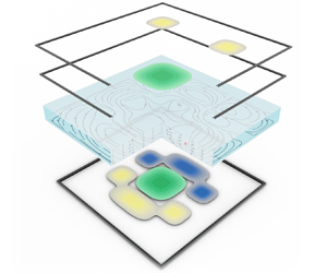
Figure 1. Illustration of a Hele-Shaw cell geometry under electric field actuation. (a) The upper and lower walls are separated by a spacing $h$, and can both exhibit non-uniform electroosmotic mobilities $\mu$ as well as slip lengths $\beta$. The resulting flow field is non-homogeneous. (b) A dissolved species, here represented by a single molecule, is transported by cross-stream diffusion and in-plane advection as well as diffusion. (c) Two-dimensional representation of the system. A concentration field distribution (red) gets dispersed over the Hele-Shaw cell. The effects of velocity inhomogeneities over the cell height are included in the dispersion matrix ${\boldsymbol{\mathsf{D}}}$, resulting in a two-dimensional model.

The transport of a dissolved species inside such a flow field is driven by advection with the background flow velocity, as well as by molecular diffusion due to Brownian motion of the molecules, as shown in figure 1(b). Assuming a sufficiently low species concentration as well as impermeable walls and no sources or sinks of concentration, e.g. due to chemical reactions or adsorption processes, the transport is governed by the 3-D advection–diffusion equation

(2.2)\begin{equation} \frac{\partial c}{\partial t} + u \frac{\partial c}{\partial x} + v \frac{\partial c}{\partial y} + w \frac{\partial c}{\partial z} = D \left( \frac{\partial^{2} c}{\partial x^{2}} +\frac{\partial^{2} c}{\partial y^{2}} +\frac{\partial^{2} c}{\partial z^{2}} \right), \end{equation}

where $D$ denotes the coefficient of molecular diffusion of the species, and $c$ the molecular concentration. While the specific boundary conditions at the outer perimeter of the cell in $x$,$y$-directions depend on the problem under study and are not important for the derivation of the transport model, we can impose the impermeability wall boundary condition at the upper and lower wall as

(2.3)\begin{equation} \frac{\partial c}{\partial z} = 0 \quad \text{at} \ z = 0,h. \end{equation}

While (2.2) represents the transport equation for the full problem, solving it for extended fluid domains can be computationally very demanding, since in all three dimensions the processes occurring on the smallest scales need to be resolved. Especially when solving transient problems, it can become impractical to compute the time evolution of the concentration field in a reasonable time. Therefore, we develop a reduced-order model that captures the processes on the small scales such that only the macro scales have to be resolved. In figure 1(c), the corresponding 2-D model of the system depicted in figure 1(a) is represented schematically.

In order to apply the multiple-scale perturbation approach, the micro- and macroscales, and thus the different time scales, need to be identified (Mei & Vernescu Reference Mei and Vernescu2010). In agreement with previous work on hydrodynamic dispersion in channels (Chu et al. Reference Chu, Garoff, Przybycien, Tilton and Khair2019), we here identify the length and time scales in a fluid domain with a typical length scale in the $x$ and $y$-directions $L$ much larger than the channel height $h$. It is important to note that the in-plane scale $L$ is due to an inhomogeneity of the flow domain on this scale, not necessarily identical to the side length of the cell. This yields a small parameter

(2.4)\begin{equation} \epsilon = \frac{h}{L} \ll 1, \end{equation}

which we will use in the perturbation analysis.

The species transport in the considered Hele-Shaw cells results in three distinct time scales. We assume that the shortest time scale is due to the diffusion in cross-stream direction, which is of the order

(2.5)\begin{equation} T_{dif,h} = O \left( \frac{h^{2}}{D} \right) = O (T_{osc}). \end{equation}

Here, in analogy to Chu et al. (Reference Chu, Garoff, Przybycien, Tilton and Khair2019), the oscillation of the flow field is considered to occur on the order of the smallest time scales, for the case that the flow field has an oscillatory component. This assumption is supported by an order-of-magnitude comparison to recent results on the topic of flow shaping, where channel heights of the order of $10^{-5}$ m were used, which in conjunction with diffusion coefficients of $10^{-9}$ m$^{2}$ s$^{-1}$ leads to $T_{dif,h} = \mathit {O} ( 10^{-1}$ s), coinciding with reported oscillatory frequencies (Paratore et al. Reference Paratore, Bacheva, Kaigala and Bercovici2019a; Dehe et al. Reference Dehe, Rofman, Bercovici and Hardt2020).

The second time scale of the system can be identified as the time scale of advection along the in-plane inhomogeneity scale $L$, resulting in

(2.6)\begin{equation} T_{adv} = O \left( \frac{L}{U_{c}} \right) = O \left( \frac{h}{W_{c}} \right) = \frac{T_{dif,h}}{\epsilon}. \end{equation}

Here, $U_{c}$ and $W_{c}$ are typical in-plane and transverse velocities, respectively. The relation of the time scales of advection in the streamwise and transverse directions can be inferred from an order-of-magnitude analysis of the continuity equation, as shown in Appendix B.

The third time scale is the diffusive time scale across the inhomogeneity scale $L$, yielding

(2.7)\begin{equation} T_{dif,L} = O \left( \frac{L^{2}}{D} \right) = \frac{T_{dif,h}}{\epsilon^{2}}. \end{equation}

Having identified all relevant time scales of the problem, a hierarchy of time variables can be defined, which we will use to perform a perturbation analysis

(2.8a–c)\begin{equation} t_0 = t, \quad t_1 = \epsilon t, \quad t_2 = \epsilon^{2} t. \end{equation}

Before we proceed, we non-dimensionalize the advection–diffusion equation (2.2). The spatial coordinates can be rescaled by the typical length scales $L$ and $h$ for the $x$ and $y$, and $z$ directions, respectively, and the velocities by their characteristic velocities $U_{c}$ and $W_{c}$. The concentration can be rescaled by a typical concentration $c_0$, and the time by the diffusive time scale $T_{dif,h}$, resulting in

(2.9)$$\begin{gather} \frac{\partial \hat{c}}{\partial \hat{t}} + \epsilon Pe \left( \frac{\partial \hat{c}}{\partial \hat{x}} + \frac{\partial \hat{c}}{\partial \hat{y}} + \frac{\partial \hat{c}}{\partial \hat{z}} \right) = \epsilon^{2} \left( \frac{\partial^{2} \hat{c}}{\partial \hat{x}^{2}} +\frac{\partial^{2} \hat{c}}{\partial \hat{y}^{2}} \right) +\frac{\partial^{2} \hat{c}}{\partial \hat{z}^{2}}, \end{gather}$$

(2.10)$$\begin{gather}\frac{\partial \hat{c}}{\partial \hat{z}} = 0 \quad \text{at} \ \hat{z} = 0,1. \end{gather}$$

Here, the hatted variables represent non-dimensionalized quantities, and $Pe$ represents the Péclet number, herein defined as $Pe = U_{c} h / D$. The advection–diffusion equation (2.9) is representative of the full problem, and in the following, we will reduce it to an effective 2-D model, governing the long-time behaviour of the full problem, following the approach by Chu et al. (Reference Chu, Garoff, Przybycien, Tilton and Khair2019).

First, we utilize the time scales defined in (2.8a–c) to expand the time derivative as

(2.11)\begin{equation} \frac{\partial}{\partial t} = \frac{\partial}{\partial t_0} + \epsilon\frac{\partial}{ \partial t_1} +\epsilon^{2} \frac{\partial}{ \partial t_2}. \end{equation}

For brevity, in what follows we have dropped the hats and all variables will be non-dimensional. The concentration field can be expanded in $\epsilon$ as (Fife & Nicholes Reference Fife and Nicholes1975)

(2.12)\begin{align} c(x,y,z,t) &= c^{(0)}(x,y,z,t_0,t_1,t_2) + \epsilon c^{(1)}(x,y,z,t_0,t_1, t_2) \nonumber\\ &\quad + \epsilon^{2} c^{(2)}(x,y,z,t_0,t_1, t_2) + O (\epsilon^{3}). \end{align}

Inserting (2.11) and (2.12) into the governing equation (2.9) and boundary condition (2.10) results in a set of equations of different orders in $\epsilon$. We will consider them in increasing order, to build up a macroscale transport equation. Before we derive the macrotransport equation, it is important to note that the components $c^{(1)}$ and $c^{(2)}$ are assumed to be fluctuating components, with vanishing average over the channel height, when averaged over one oscillation period. The details of this rationale will be outlined and justified during the derivation of the macrotransport equation. Additionally, in § 2.4 we will sketch how the derivation would change if this assumption was not introduced.

2.2. Leading-order perturbation: $\mathit {O} = ( \epsilon ^{0} )$

The leading-order approximation results in

(2.13)$$\begin{gather} \frac{\partial c^{(0)}}{\partial t_0} = \frac{\partial^{2} c^{(0)}}{\partial z^{2}}, \end{gather}$$

(2.14)$$\begin{gather}\frac{\partial c^{(0)}}{\partial z} = 0 \quad \text{at } z = 0,1. \end{gather}$$

The solution to (2.13) under the boundary condition (2.14) can be expressed as a infinite series of the form

(2.15)\begin{equation} c^{(0)} = c^{(0)}_0 (x,y,t_1,t_2) + \sum_{n=1}^{\infty} c^{(0)}_n(x,y,t_1,t_2) \ \textrm{e}^{{-}n^{2}{\rm \pi}^{2} t_0} \cos (n{\rm \pi} z). \end{equation}

If the initial distribution $c^{(0)}$ depends on $z$, the $z$-dependent terms decay over a time scale $t_0$ due to the factor $\textrm {e}^{-n^{2}{\rm \pi} ^{2} t_0}$, and are thus irrelevant for the long-term solution. Therefore, it is legitimate to drop the dependence on $t_0$ and utilize

(2.16)\begin{equation} c^{(0)} = c^{(0)}_0 (x,y,t_1,t_2). \end{equation}

The independence of $c^{(0)}$ from the transverse coordinate $z$ indicates that it represents the cross-stream average of the concentration.

2.3. First-order perturbation: $\mathit {O} = ( \epsilon ^{1} )$

The first-order perturbation of (2.9) under the boundary condition (2.10) yields

(2.17)$$\begin{gather} \frac{\partial c^{(0)}}{\partial t_1} + \frac{\partial c^{(1)}}{\partial t_0} + Pe \,u \frac{\partial c^{(0)}}{\partial x} + Pe\, v \frac{\partial c^{(0)}}{\partial y}= \frac{\partial^{2} c^{(1)}}{\partial z^{2}}, \end{gather}$$

(2.18)$$\begin{gather}\frac{\partial c^{(1)}}{\partial z} = 0 \quad \text{at } z = 0,1. \end{gather}$$

In order to derive the macroscale transport equation, let us introduce the time average over one period of oscillation (on the short time scale) as

(2.19)\begin{equation} \overline{({\cdot})} = \frac{1}{T_{osc}} \int_{t_0}^{t_0 + T_{osc}} ({\cdot}) \,\mathrm{d} t_0, \end{equation}

and the transverse average as

(2.20)\begin{equation} \langle ({\cdot}) \rangle = \int_0^{1} ({\cdot}) \,\mathrm{d} z. \end{equation}

Applying now both the time and transverse average to (2.17) leads to an equation for $c^{(0)}$ on time scale $t_1$ as

(2.21)\begin{equation} \frac{\partial c^{(0)}}{\partial t_1} + Pe \langle \bar{u} \rangle \frac{\partial c^{(0)}}{\partial x} + Pe \langle \bar{v} \rangle \frac{\partial c^{(0)}}{\partial y}= 0, \end{equation}

where the term on the right-hand side vanishes due to the time average of the boundary condition (2.18), and the second term on the left-hand side due to the averaging over a fluctuating component, as discussed in the preceding section. Physically, this equation demonstrates that the development of the height-averaged concentration $c^{(0)}$ is driven by the advection with the average flow velocity, in accordance with our initial assumptions in § 2.1.

In order to obtain $c^{(1)}$, we can subtract (2.21) from (2.17), insert (2.1), resulting in an expression for $c^{(1)}$ as

(2.22)\begin{equation} \frac{\partial c^{(1)}}{\partial t_0} + Pe ( ( \bar{u} - \langle \bar{u} \rangle ) + u' ) \frac{\partial c^{(0)}}{\partial x} + Pe ( (\bar{v} - \langle \bar{v} \rangle ) + v' ) \frac{\partial c^{(0)}}{\partial y}= \frac{\partial^{2} c^{(1)}}{\partial z^{2}}. \end{equation}

This equation can be interpreted as the governing equation for the cross-stream concentration variation $c^{(1)}$, which is driven by velocity variations over the channel height, relative to the time and transverse average. It is visible that two contributions drive the system. One is due to the time-averaged velocity differences over the channel height $(\bar {u} - \langle \bar {u} \rangle ,\bar {v} - \langle \bar {v} \rangle )$, and the other one due to the oscillatory velocities ($u',v'$). Due to the linearity of the equation, $c^{(1)}$ is expected to consist of a stationary part and an oscillatory part, and (2.22) suggests the form

(2.23)\begin{equation} c^{(1)} = Pe ( \boldsymbol{a}(x,y,z) + \boldsymbol{b}(x,y,z,t_0) ) \boldsymbol{\cdot} \boldsymbol{\nabla}_\parallel c^{(0)}. \end{equation}

Here, we have introduced the streamwise gradient $\boldsymbol {\nabla }_\parallel = (\partial /\partial x, \partial / \partial y)$ to simplify notation. Based on the assumption that $c^{(1)}$ is a fluctuation quantity, contributions from the general solution of the homogeneous equation were neglected in the above ansatz.

The stationary solution $\boldsymbol {a}$ and the oscillatory solution $\boldsymbol {b}$ are governed by two separate problems, which we can obtain by inserting (2.23) into (2.22), and separating the stationary problem and the oscillatory problem. The corresponding boundary conditions for $\boldsymbol {a}$ and $\boldsymbol {b}$ are found by inserting (2.23) into the boundary condition (2.18). The problem associated with the steady-state term then reads

(2.24)\begin{equation} \begin{pmatrix} \bar{u} - \langle \bar{u} \rangle\\ \bar{v} - \langle \bar{v} \rangle \end{pmatrix}= \frac{\partial^{2} \boldsymbol{a}}{\partial z^{2}}, \quad \text{with} \ \frac{\partial \boldsymbol{a}}{\partial z} = 0 \ \text{at} \ z = 0,1. \end{equation}

From the structure of (2.24), we can see that the solution is not unique. If $\boldsymbol {a}^{(1)}$ is a solution of (2.24), then $\boldsymbol {a}^{(1)} + \boldsymbol {C}(x,y)$ satisfies the equation as well, where $\boldsymbol {C}(x,y)$ is an arbitrary function depending on $x$, $y$ only. Therefore, in order to render the solution unique, we can impose the additional condition $\langle \boldsymbol {a} \rangle = \boldsymbol {0}$. As we have pointed out in § 2.1, $c^{(1)}$ is expected to be a fluctuating quantity, and by imposing the aforementioned condition, we ensure that the stationary component of (2.23) satisfies this condition.

In a similar manner, the unsteady problem associated with $\boldsymbol {b}$ is obtained as

(2.25)\begin{equation} \frac{\partial \boldsymbol{b}}{\partial t_0} + \begin{pmatrix} u'\\ v' \end{pmatrix} = \frac{\partial^{2} \boldsymbol{b}}{\partial z^{2}}, \quad \text{with} \ \frac{\partial \boldsymbol{b}}{\partial z} = 0 \ \text{at} \ z = 0,1. \end{equation}

As we can see, this equation does not uniquely define $\boldsymbol {b}$. If $\boldsymbol {b^{(1)}}$ is a solution to (2.25), then $\boldsymbol {b^{(1)}} + \boldsymbol {D}(x,y)$ is a solution as well, where $\boldsymbol {D}(x,y)$ is an arbitrary function depending on $x$ and $y$ only. In order to render the solution unique, we impose the additional condition $\langle \bar {\boldsymbol {b}} \rangle = \boldsymbol {0}$. In analogy to the additional condition for $\boldsymbol {a}$, we ensure that $c^{(1)}$ is a fluctuating component, vanishing upon time and height averaging. The solutions to both boundary value problems (2.24) and (2.25) depend on the specific flow field and, for now, we will keep it in the general form. We will discuss some specific solutions in § 5. For now, we just assume that we have solved for $\boldsymbol {a}$ and $\boldsymbol {b}$, and thus determined $c^{(1)}$, allowing us to move on to the second-order perturbation.

2.4. Second-order perturbation: $\mathit {O} = ( \epsilon ^{2} )$

For the order $\mathit {O} = ( \epsilon ^{2} )$, we first identify the governing equation as

(2.26)\begin{align} &\frac{\partial c^{(0)}}{\partial t_2} + \frac{\partial c^{(1)}}{\partial t_1} + \frac{\partial c^{(2)}}{\partial t_0} + Pe \left( u \frac{\partial c^{(1)}}{\partial x} + v \frac{\partial c^{(1)}}{\partial y} + w \frac{\partial c^{(1)}}{\partial z} \right)\nonumber\\ &\quad = \frac{\partial^{2} c^{(0)}}{\partial x^{2}} + \frac{\partial^{2} c^{(0)}}{\partial y^{2}} +\frac{\partial^{2} c^{(2)}}{\partial z^{2}}, \end{align}

and the boundary conditions as

(2.27)\begin{equation} \frac{\partial c^{(2)}}{\partial z} = 0 \quad \text{at } z = 0,1. \end{equation}

As we can see from (2.26), $c^{(2)}$ exhibits an ambiguity as well. In analogy to $\boldsymbol {a}$ and $\boldsymbol {b}$, we impose the additional restriction that $c^{(2)}$ is a fluctuation quantity, i.e. $\langle \overline {c^{(2)}} \rangle = 0$. Thus, the time and transverse average of the third term of (2.26) disappears.

Our choice of the additional conditions to render the solutions unique becomes more clear in retrospect, since now $c^{(0)}$ represents the long-term, cross-stream average of the concentration distribution. The components $c^{(i)}$ for $i\geq 1$ are fluctuating components that vanish upon transverse and time averaging (Mei, Auriault & Ng Reference Mei, Auriault and Ng1996; Chu et al. Reference Chu, Garoff, Przybycien, Tilton and Khair2019). If we had chosen different constraints for $\boldsymbol {a}$, $\boldsymbol {b}$ and $c^{(2)}$, leading to a non-vanishing time and height average of $c^{(1)}$ or $c^{(2)}$, we could carry out the derivation including these additional terms. As a result, $c^{(0)}$ would not represent the long-time height average, but we would have to use the fact that $\langle \bar {c} \rangle = \langle \overline {c^{(0)}} \rangle + \epsilon \langle \overline {c^{(1)}} \rangle +\epsilon ^{2} \langle \overline {c^{(2)}} \rangle$ to rewrite the final macrotransport equation. In the current derivation, we obtain the macrotransport equation in terms of $c^{(0)}$, thus simplifying it significantly.

The details of the simplification of the terms in (2.26) can be looked up in Appendix A. Inserting (A3), (A4) and (A5) into (2.26) leads to

(2.28)\begin{align} &\frac{\partial c^{(0)}}{\partial t_2} + Pe^{2} \left( \left\langle \bar{u} \frac{\partial \boldsymbol{a}}{\partial x} \right\rangle + \left\langle \bar{v} \frac{\partial \boldsymbol{a}}{\partial y} \right\rangle + \left\langle \bar{w} \frac{\partial \boldsymbol{a}}{\partial z} \right\rangle + \left\langle \overline{u' \frac{\partial \boldsymbol{b}}{\partial x}} \right\rangle + \left\langle \overline{v' \frac{\partial \boldsymbol{b}}{\partial y}} \right\rangle + \left\langle \overline{w' \frac{\partial \boldsymbol{b}}{\partial z}} \right\rangle \right) \boldsymbol{\cdot} \boldsymbol{\nabla}_\parallel c^{(0)} \nonumber\\ &\qquad + Pe^{2} \left( \langle \bar{u} \boldsymbol{a}\rangle \boldsymbol{\cdot} \frac{\partial \boldsymbol{\nabla}_\parallel c^{(0)}}{\partial x} + \langle \bar{v} \boldsymbol{a}\rangle \boldsymbol{\cdot} \frac{\partial \boldsymbol{\nabla}_\parallel c^{(0)}}{\partial y} + \langle \overline{u' \boldsymbol{b}}\rangle \boldsymbol{\cdot} \frac{\boldsymbol{\nabla}_\parallel c^{(0)}}{\partial x} +\langle \overline{v' \boldsymbol{b}}\rangle \boldsymbol{\cdot} \frac{\boldsymbol{\nabla}_\parallel c^{(0)}}{\partial y}\right) \nonumber\\ &\quad=\nabla_\parallel^{2} c^{(0)}. \end{align}

2.5. Final macrotransport equation

The final macrotransport equation is obtained by adding (2.28) multiplied by $\epsilon ^{2}$ to (2.21) multiplied by $\epsilon$ and using $t_i = \epsilon ^{i} t$. This results in

(2.29)\begin{align} &\frac{\partial c^{(0)}}{\partial t} + (\epsilon Pe \langle \bar{\boldsymbol{u}}_\parallel \rangle + \epsilon^{2} Pe^{2} ( \boldsymbol{k}_{stat} + \boldsymbol{k}_{osc} ))\boldsymbol{\cdot} \boldsymbol{\nabla}_\parallel c^{(0)}\nonumber\\ &\quad = \epsilon^{2} (\boldsymbol{\nabla}_\parallel \boldsymbol{\cdot} [ ( {\boldsymbol{\mathsf{I}}} - Pe^{2} {\boldsymbol{\mathsf{D}}} ) \boldsymbol{\cdot} \boldsymbol{\nabla}_\parallel c^{(0)}]), \end{align}

where we have subsumed the velocity components in the $x$ and $y$-directions into $\bar {\boldsymbol {u}}_\parallel = (\bar {u},\bar {v})$. Here, $\boldsymbol {k}_{stat}$ and $\boldsymbol {k}_{osc}$ denote advection-correction terms due to the stationary flow field and the oscillatory flow field, respectively, ${\boldsymbol{\mathsf{I}}}$ denotes the identity matrix and ${\boldsymbol{\mathsf{D}}}$ the dispersion tensor. The advection-correction terms are given as

(2.30)\begin{equation} \boldsymbol{k}_{stat} ={-}\left\langle \frac{\partial \bar{u}}{\partial x} \boldsymbol{a} \right\rangle -\left\langle \frac{\partial \bar{v}}{\partial y} \boldsymbol{a} \right\rangle +\left\langle \bar{w} \frac{\partial \boldsymbol{a}}{\partial z} \right\rangle \end{equation}

and

(2.31)\begin{equation} \boldsymbol{k}_{osc} ={-}\left\langle \overline{ \frac{\partial u'}{\partial x} \boldsymbol{b} } \right\rangle -\left\langle \overline{ \frac{\partial v'}{\partial y} \boldsymbol{b} } \right\rangle + \left\langle \overline{w' \frac{\partial \boldsymbol{b}}{\partial z} } \right\rangle, \end{equation}

and the dispersion tensor is given as

(2.32)\begin{equation} {\boldsymbol{\mathsf{D}}} = {\boldsymbol{\mathsf{D}}}_{stat} + {\boldsymbol{\mathsf{D}}}_{osc} =\begin{bmatrix} \langle \bar{u} a_x \rangle & \langle \bar{v} a_x \rangle \\ \langle \bar{u} a_y \rangle & \langle \bar{v} a_y \rangle \end{bmatrix} + \begin{bmatrix} \langle \overline{u' b_x}\rangle & \langle \overline{v' b_x}\rangle \\ \langle \overline{u' b_y}\rangle & \langle \overline{v' b_y}\rangle \end{bmatrix}. \end{equation}

Note that the subscripts $x$, $y$ denote vector components of $\boldsymbol {a}$ and $\boldsymbol {b}$.

Only the spatial coordinates $x$ and $y$ enter the macroscale transport equation (2.29), and the time-averaged effects due to cross-stream transport are contained in the transport coefficients (2.30, 2.31 and 2.32). Once the problems (2.24) and (2.25) have been solved, all coefficients of (2.29) are determined. The different terms can be interpreted as advection with the mean flow (second term on the left-hand side), an advection-correction term due to the variation of the flow with $z$ for stationary ($\boldsymbol {k}_{stat}$) and oscillatory flow ($\boldsymbol {k}_{osc}$), molecular diffusion (first term on right-hand side) and Taylor–Aris dispersion due to stationary (${\boldsymbol{\mathsf{D}}}_{stat}$) and oscillatory (${\boldsymbol{\mathsf{D}}}_{osc}$) flow. Similarly to previously reported dispersion models (e.g. Watson Reference Watson1983), the dispersion effects due to the stationary and the oscillatory component are additive. Also, the dispersion tensor exhibits a pre-factor $-Pe^{2}$, which we have to keep in mind when discussing the dispersion in specific flow fields in §§ 4 and 5. In addition to the derivation presented here, a similar equation can be derived using scaling arguments, following the classical analysis of Taylor–Aris dispersion. This alternative derivation is presented in the supplementary material (see supplementary material available at https://doi.org/10.1017/jfm.2021.648) for the case of stationary flow.

2.6. Thermodynamic consistency of the dispersion tensor

In order to fulfil the second law of thermodynamics, the dispersion tensor ${\boldsymbol{\mathsf{I}}}-Pe^{2}{\boldsymbol{\mathsf{D}}}$ (2.32) has to be positive definite. As we have discussed, a dispersion tensor can instantaneously exhibit negative eigenvalues when the flow contracts a concentration field (Smith Reference Smith1982). The time-averaged dispersion tensor, however, has to be positive definite, in order to be able to apply (2.29) without the occurrence of singularities in the concentration.

A positive definite tensor ${\mathsf{A}}_{ij}$ fulfils the condition $\chi _i {\mathsf{A}}_{ij}\chi _j>0$ (in index notation, using the Einstein summation convention), where $\boldsymbol {\chi }$ represents an arbitrary vector. We have to show that

(2.33)\begin{equation} \chi_i (\delta_{ij}-Pe^{2} ({\mathsf{D}}_{\text{stat},ij} + {\mathsf{D}}_{\text{stat},ij})) \chi_j>0 \end{equation}

is satisfied, where the identity tensor is expressed by the Kronecker delta $\delta_{ij}$. The first term is positive definite, as $\chi _i \delta_{ij} \chi _j=(\chi _k )^{2}>0$.

In order to evaluate the stationary dispersion component, we rewrite ${\boldsymbol{\mathsf{D}}}_{stat}$ as

(2.34)\begin{equation} {\mathsf{D}}_{stat,ij} = \langle \overline{u}_i a_j \rangle = \langle a_j ( \overline{u}_i - \langle\overline{u}_i \rangle ) \rangle = \left\langle a_j \frac{\partial^{2} a_i}{\partial z^{2}} \right\rangle , \end{equation}

where we have used (2.24). Integration by parts and using the boundary condition from (2.24) leads to

(2.35)\begin{equation} \left\langle a_j \frac{\partial^{2} a_i}{\partial z^{2}} \right\rangle = \left[ \frac{\partial a_i}{\partial z} a_j \right]_{z=0}^{1} - \left\langle \frac{\partial a_j}{\partial z} \frac{\partial a_i}{\partial z} \right\rangle ={-} \left\langle \frac{\partial a_j}{\partial z} \frac{\partial a_i}{\partial z} \right\rangle. \end{equation}

Then, we can show that the stationary component is positive semi-definite,

(2.36)\begin{align} \chi_i (- Pe^{2} {\mathsf{D}}_{\text{stat},ij}) \chi_j &= Pe^{2} \chi_i \left\langle \frac{\partial a_i}{\partial z} \frac{\partial a_j}{\partial z} \right\rangle \chi_j = Pe^{2} \left\langle \chi_i \frac{\partial a_i}{\partial z} \chi_j \frac{\partial a_j}{\partial z} \right\rangle \nonumber\\ &= Pe^{2} \left\langle \left( \frac{\partial a_k}{\partial z} \chi_k \right)^{2} \right\rangle \geq 0, \end{align}

becoming zero only if $\boldsymbol {a}$ vanishes everywhere. This case corresponds to the situation of vanishing dispersion.

Next, we rewrite the oscillatory component as

(2.37)\begin{equation} {\mathsf{D}}_{osc,ij}= \langle \overline{b_i u'_j } \rangle = \left\langle\overline{ b_i \left(-\frac{\partial b_j}{\partial t_0} + \frac{\partial^{2} b_j}{\partial z^{2}} \right) } \right\rangle ={-}\left\langle\overline{ b_i \frac{\partial b_j}{\partial t_0}} \right\rangle + \left\langle\overline{ b_i \frac{\partial^{2} b_j}{\partial z^{2}} } \right\rangle, \end{equation}

where we have used (2.25). Analogously to the stationary component, we can show that the second term on the right-hand side is positive semi-definite. The first term of (2.37) inserted into (2.33) leads to

(2.38)\begin{align} \chi_i \left\langle - \overline{b_j \frac{\partial b_j}{\partial t_0}} \right\rangle \chi_j &={-}\left\langle\overline{\frac{1}{2}\chi_x^{2} \frac{\partial b_x^{2}}{\partial t_0}} \right\rangle - \left\langle\overline{\frac{1}{2}\chi_y^{2} \frac{\partial b_y^{2}}{\partial t_0}} \right\rangle - \left\langle\chi_x \chi_y\overline{ \frac{\partial b_x}{\partial t_0} b_y} + \chi_x \chi_y\overline{\frac{\partial b_y}{\partial t_0} b_x } \right\rangle\nonumber\\ &={-}\left\langle\overline{\frac{1}{2}\chi_x^{2} \frac{\partial b_x^{2}}{\partial t_0}} \right\rangle - \left\langle\overline{\frac{1}{2}\chi_y^{2} \frac{\partial b_y^{2}}{\partial t_0}} \right\rangle\nonumber\\ &\quad - \left\langle\chi_x \chi_y \left( \frac{1}{T_{osc}}[b_x b_y ]_{t_0}^{t_0+T_{osc}} -\overline{ \frac{\partial b_y}{\partial t_0} b_x } + \overline{\frac{\partial b_y}{\partial t_0} b_x } \right)\right\rangle =0. \end{align}

Keeping in mind that $\boldsymbol {b}$ is an oscillatory function, as follows from the definition (2.25), we see that the final expression vanishes. Collecting all contributions, it follows that the condition (2.33) is satisfied, leading to a positive definite dispersion tensor.

3.1. Form of the solution for a stationary flow field

From the derivation in Appendix B, it is clear that a stationary flow field takes the form of a quadratic polynomial. In the following, we express the stationary dispersion tensor using a corresponding parametrization of the velocity field,

(3.10a)$$\begin{gather} u(x,y,z) = A_1(x,y) z^{2} + A_2(x,y) z + A_3(x,y), \end{gather}$$

(3.10b)$$\begin{gather}v(x,y,z) = B_1(x,y) z^{2} + B_2(x,y) z + B_3(x,y). \end{gather}$$

Then, by solving equation (2.24), the stationary dispersion tensor follows from (2.32) as

(3.11)\begin{align} {\boldsymbol{\mathsf{D}}}_{stat} = \begin{bmatrix} -\dfrac{8 A_1^{2}}{945} - \dfrac{A_1 A_2}{60} - \dfrac{A_2^{2}}{120} & -\dfrac{8 A_1 B_1}{945} - \dfrac{A_2 B_1}{120} - \dfrac{A_1 B_2}{120} - \dfrac{A_2 B_2}{120} \\[8pt] -\dfrac{8 A_1 B_1}{945} - \dfrac{A_2 B_1}{120} - \dfrac{A_1 B_2}{120} - \dfrac{A_2 B_2}{120} & -\dfrac{8 B_1^{2}}{945} - \dfrac{B_1 B_2}{60} - \dfrac{B_2^{2}}{120} \end{bmatrix}, \end{align}

and the advection-correction term from (2.30) as

(3.12)\begin{align} \boldsymbol{k}_{stat}= \begin{bmatrix} \dfrac{1}{2160} (16 A_1 + 15 A_2) \left(2 \dfrac{\partial A_1 }{\partial x} + 3 \dfrac{\partial A_2}{ \partial x} + 6 \dfrac{\partial A_3}{ \partial x} + 2 \dfrac{\partial B_1}{ \partial y} + 3 \dfrac{\partial B_2}{ \partial y} + 6 \dfrac{\partial B_3}{ \partial y}\right)\\ \dfrac{1}{2160} (16 B_1 + 15 B_2) \left(2 \dfrac{\partial A_1}{ \partial x} + 3 \dfrac{\partial A_2}{ \partial x} + 6 \dfrac{\partial A_3 }{ \partial x} + 2 \dfrac{\partial B_1}{ \partial y} + 3 \dfrac{\partial B_2}{ \partial y} + \dfrac{6 \partial B_3}{ \partial y}\right) \end{bmatrix}. \end{align}

5.1. Numerical methods

Among others, the dispersion model is motivated by the need to reduce the dimensionality of the problem, so that concentration fields in Hele-Shaw flows can be computed efficiently. Numerical simulations including all three dimensions require a sufficient resolution to resolve the processes on the small scale (over the cell height), thus rendering the computational problem much more expensive. In order to evaluate the accuracy of the dispersion model, we compare concentration fields obtained with this model with fields resulting from a particle-tracking method in a 3-D domain using Comsol Multiphysics 5.5. For the 3-D computations, a particle approach is used rather than a continuum method, since it is less prone to discretization errors at high Péclet numbers (numerical diffusion). For the presented test cases, we extract the concentration distributions obtained with both approaches and compare them to assess the validity of the dispersion model.

5.2. Test case A: dispersion due to a stationary flow field

In order to validate the stationary part of the dispersion model, we analyse a steady-state flow field with zero average flow velocity. We achieve that by imposing wall mobilities with opposite signs ($\mu ^{U} = -\mu ^{L}$) at the upper and lower walls of the cell, without any external pressure gradient. By imposing periodic boundary conditions, the resulting flow field is a shear flow, as indicated in figure 5(a). It is worth pointing out that due to the absence of a height-averaged velocity, the only remaining contributions in the macrotransport equation (2.29) are the time derivative of the concentration field and the effective diffusivities on the right-hand side. The dispersion coefficients are calculated according to the governing equations described in § 2.3.

Figure 5. Test case A: comparison of hydrodynamic dispersion inside a Hele-Shaw cell as obtained with the 2-D dispersion model (c–e) and 3-D particle-tracking simulations (f–h). (a) The system consists of a Hele-Shaw cell with wall mobilities of opposite sign at the bounding walls, leading to a shear flow with zero average flow velocity. (b) An initial concentration distribution is dispersed over time, and the resulting concentration distributions are shown after a time span of $70.59 \,T_{dif,h}$ (c–h). The direction of the electric field is indicated at the top-right corner of each panel.

The parameters chosen for the calculations are shown in table 2. We compute the dispersion for three cases with the same magnitude of the electric field but different directions, while maintaining the mobility at the walls and the initial concentration distribution. This allows probing of the off-diagonal components of the dispersion tensor. The initial concentration distribution is of square shape, where the edges were smoothed using an error function, as described in the supplementary material.

Table 2. Parameter values used in the calculations of test cases A and B, as indicated in figures 5 and 6. Additional information on the initial conditions is presented in Appendix D and the supplementary material.

In figure 5, the resulting concentration distributions from the 2-D dispersion model (c–e) and the 3-D particle simulations are shown (f–h). In the upper right corner, the direction of the electric field is indicated. First, we would like to discuss the 3-D simulation data, which are less smooth than the 2-D results. The concentration field is extracted on a mesh of $60\times 60$ cells, and the initial concentration inside the rectangle corresponds to 142 particles per cell. We have chosen not to smooth the data, in order to prevent an artificial broadening of the mixing zones. Apart from local inhomogeneities, the agreement between the 2-D and the 3-D calculations is evident. In the direction of the flow, dispersion enhances mass transport. To quantify the extent of the mixing regions and compare how well the dispersion model reproduces the 3-D simulations, we take the case of an electric field in the $x$-direction as an example (figure 5c,f). We define the boundary of the concentration distribution as the value $x_0$ where $c(x_0)=0.1$. The size of the region for the dispersion model is denoted by $x_{0,2D}$, and for the particle simulations by $x_{0,3D}$. The size of the concentration field broadened by dispersion exhibits a relative error of $(x_{0,2D}-x_{0,3D})/x_{0,3D} = 7.4\,\%$ on average inside the central region ($\vert y \vert < 0.1$). In the $y$-direction (perpendicular to the electric field), the relative error yields 2.5 % on average. The extent of the zones broadened by dispersion agrees well between the calculations, and in the direction normal to the flow velocity, molecular diffusion is much weaker, leading to a much smaller diffusive broadening. These results show that the dispersion due to a stationary flow field is captured by the 2-D model.

5.3. Test case B: dispersion due to a oscillatory flow field

In order to validate the oscillatory part of the dispersion model, we analyse a similar case as in the preceding section, resulting in a shear flow field with zero average flow velocity. However, we modify the velocity by multiplying it with a factor $\sin (2 {\rm \pi}f t)$, as indicated in figure 6. As a result, the flow field becomes oscillatory, where both $\langle \bar {\boldsymbol {u}} \rangle$ and $\bar {\boldsymbol {u}}$ vanish.

Figure 6. Test case B: comparison of dispersion inside a Hele-Shaw cell due to oscillatory flow obtained from the 2-D dispersion model (c–e) and 3-D particle-tracking simulations (f–h). (a) The wall mobilities are of opposite signs and the flow is actuated by an oscillatory electric field oriented along the $x$-axis, leading to a shear flow with zero time average. (b) Initial concentration field as used for the computations. (c–h) The resulting concentration distributions are shown after a time span of $70.59 \,T_{dif,h}$. The oscillation frequency is indicated inside each panel.

Before discussing the resulting concentration distribution, we would like to outline some analogies between the dispersion due to oscillatory flow and due to stationary flow. As evident from the macroscale transport equation, for each stationary term (denoted by some function of the time averaged flow field $\boldsymbol {u}$ and $\boldsymbol {a}$), a corresponding oscillatory term exists (denoted by some function of the oscillatory flow field $\boldsymbol {u}'$ and $\boldsymbol {b}$). That is, dispersion can either be driven by a flow field that is non-uniform over $z$ but stationary, or by a flow field non-uniform over both $z$ and $t$.

Solving the boundary value problem for $\boldsymbol {b}$ is more complex than the analogous stationary problem for $\boldsymbol {a}$ outlined in the preceding section, since $\boldsymbol {b}$ exhibits a time dependence, but it is straightforward and can be done numerically. In figure 7, we show the resulting dispersion coefficient $\langle \overline {u' \boldsymbol {b}}\rangle$ for varying oscillation frequencies (which are non-dimensionalized by the inverse diffusive time scale). The dispersion coefficient exhibits a behaviour previously reported (Chatwin Reference Chatwin1975; Vedel & Bruus Reference Vedel and Bruus2012; Chu et al. Reference Chu, Garoff, Przybycien, Tilton and Khair2019). For the case of slow oscillations ($f \xrightarrow {} 0$), it approaches half of the value obtained for the case of a stationary flow with the same amplitude, as we obtained for test case A. For the case of fast oscillations ($f \gg 1$), the dispersion coefficient approaches zero. The limit for slow oscillations is mathematically determined by an integral over one period of oscillation of a product of two sine functions. If the oscillatory signals exhibited a different time dependence than a harmonic one, the ratio of the oscillatory dispersion tensor components to the steady-state dispersion tensor components would differ from $1/2$, as we discussed in § 3. In the limit of fast oscillations, however, the limiting value remains $0$, since the flow oscillation occurs on time scales much faster than the diffusion time scale over the channel height.

Figure 7. Test case B: dependence of the dispersion coefficient on the oscillation frequency. In the limit of fast oscillations, the dispersion coefficient tends to zero, in the limit of slow oscillations, it converges to one half of the value obtained for a stationary flow of the same magnitude.

Since we have already demonstrated in test case A that the directional dependence of the dispersion tensor on the electric field can be captured by the model, we focus solely on the variation of the oscillatory frequencies while keeping the direction of the electric field constant. The resulting concentration fields for three different oscillatory frequencies ($\,f = 0.1, 1, 10$) are depicted in figure 6, where the electric field is aligned with the $x$-axis. The dispersion decreases with increasing frequency. At $f=0.1$, the dispersion is most pronounced, and for $f=10$, it is of the same order of magnitude as the molecular diffusion. Using the same relative error as in test case A, we characterize the extent of the concentration distributions. The resulting relative error between the 3-D and 2-D simulations is 7.6 % for $f=0.1$, 3.9 % for $f=1$ and 7.9 % for $f=10$. Again, there is a good agreement between the 2-D and the 3-D calculations, considering the local inhomogeneities of the particle simulations.

Apart from that, additional conclusions can be drawn from these results. Dispersion due to oscillations will only dominate over steady-state dispersion if the amplitude of $\boldsymbol {u}'$ is larger than that of the steady-state component $\bar {\boldsymbol {u}}$ and if additionally, the oscillation period is of the order of the diffusive time scale or larger. In other cases, the steady-state dispersion will dominate. For realistic systems devoted to flow shaping, such as reported by Paratore et al. (Reference Paratore, Bacheva, Kaigala and Bercovici2019a), the channel has a height of the order of 10 $\mathrm {\mu }$m, resulting, in combination with the assumed diffusion constant, on a diffusive time scale of seconds. Typically, such a system is operated at oscillatory frequencies of the order of several Hz, rendering it rather insensitive to dispersion due to oscillations. Motivated by such examples, we will focus on steady-state dispersion in test case C.

5.4. Test case C: inhomogeneous flow field

In this section, we would like to demonstrate the ability of the model to capture dispersion in a complex flow pattern. As outlined in the introduction, our research is motivated by the idea of shaping flows inside a microfluidic device without relying on fixed wall geometries, therefore making it reconfigurable during operation. More specifically, if the flow can be controlled both in space and time, different standard microfluidic operations can be performed consecutively, for example mixing of species and partitioning the flow to various outlet ports. In this test case, we analyse the effect of a complex flow pattern on a Hele-Shaw cell, half of which ($y>0$) is filled with a dissolved species. The parameters used in this test case are summarized in table 3.

Table 3. Values of parameter utilized in test case C, as indicated in figure 8. Additional information on the initial conditions is presented in Appendix D and the supplementary material.

In figure 8(a,b), the wall-mobility distribution is shown: at the lower wall we have two regions with the wall mobility $\mu ^{L}$ differing from zero. The mobility distribution is antisymmetric with respect to the $y$-axis. At the upper wall, the wall mobility is of opposite sign relative to the lower wall, with a magnitude reduced by a factor of 0.75 ($\mu ^{U} = -0.75\mu ^{L}$). The flow is driven by an electric field in the $x$-direction, leading to a rotational average flow field as indicated by the streamlines in figure 8(b). Different from the previous test cases, here the Hele-Shaw cell has an aspect ratio of 4:1 in the $x$–$y$ plane. We define all mobilities as well as the driving electric field to be time independent, thus the problem is governed by (3.5) and (3.8). Corresponding wall-mobility distributions can be created using different principles, such as chemical patterning (Paratore et al. Reference Paratore, Boyko, Kaigala and Bercovici2019b) or actuation by electrodes (Paratore et al. Reference Paratore, Bacheva, Kaigala and Bercovici2019a; Dehe et al. Reference Dehe, Rofman, Bercovici and Hardt2020). The boundaries at the perimeter of the cell are assumed to be periodic in the $y$-direction, with no-penetration boundaries in the $x$-direction. The rationale behind choosing such a flow field stems from the well known blinking vortex principle (Aref Reference Aref1984), where the flow field consists of two co-rotating in-plane vortices with an offset between their centres. The term blinking refers to the fact that the two vortices are switched on and off in succession. Based on such flows chaotic mixing can be achieved if the blinking period is chosen appropriately. In our case, it is expected that chaotic mixing efficiently distributes the species over the cell. However, due to computational constraints, we only analyse the initial phase of the advection–diffusion process.

Figure 8. Configuration of test case C. (a) The fluid flow is driven by a wall-mobility distribution both on the top ($\mu ^{U}$) and bottom walls of the fluidic cell ($\mu ^{L}$), where the mobilities are of opposing signs at opposing walls, and an electric field in the positive $x$-direction. The mobility at the upper plate has a magnitude of 75 % of that on the lower plate. (b) Resulting circulating flow field, depicted by streamlines of the averaged flow velocity $\langle \boldsymbol {u}_\parallel \rangle$. (c–e) The flow field leads to a dispersion tensor, where the dispersion in $x$-direction is strongly enhanced in the region of the mobility patch, while in the $y$-direction it is comparable to the molecular diffusion.

In figure 8(c–e), we depict the components of the dispersion tensor. For the dispersion coefficient in the $x$-direction, it is visible that it is strongly enhanced above the non-zero wall-mobility regions. Here, the flow has a strong shear component. Outside, molecular diffusion is the driving mechanism. The off-axis components of the dispersion matrix are much smaller than the molecular diffusion, thus having little influence. In the $y$-direction, the flow is driven by pressure gradients created by the wall mobility, but since the average flow velocity is smaller than the wall velocity in the shear region, the dispersion coefficient is close to that of molecular diffusion.

We computed the time evolution of the concentration field with the particle-tracking method in three dimensions, the dispersion model in two dimensions and additionally without dispersion, only considering molecular diffusion. In figure 9 we show the concentration field for three different points in time. At first glance, the concentration fields are comparable to each other, due to the fact that the dominant transport mechanism in this system is advection with the mean velocity. However, when comparing in detail, certain differences become apparent. Before entering the region with strong shear flow (and thus enhanced dispersion), the mixing regions between the regions with high and low concentration are nearly identical. After passing this region, the extension of the mixing zones between the yellow and blue regions is increased for the case that dispersion is included, both visible in the 2-D and 3-D data. This difference increases with time. In order to quantify the ability of the dispersion model to capture the growth of the mixing zones over time, we compute the area of the mixing zones for each time step. The area is defined as the regions depicted in figure 9, where the concentration takes the values $0.1< c<0.5$. Using only those regions that exhibit a relatively small concentration, we exclude errors due to numerical fluctuations in regions with high concentration, visible in figure 9(d,g,j), from affecting this integral measure. For the instances shown in figure 9, the dispersion model slightly overpredicts dispersion, leading to an increase of the mixing regions compared with the 3-D simulations of 6.1 %, 4.4 % and 2.1 %, respectively. If only molecular diffusion is taken into account, the mixing regions are 2.1 %, 23.6 % and 26.9 % smaller than in the 3-D simulations. In the supplementary material, we provide an image where the spatial distribution of the mixing zones is depicted. It is also worth noting that concentration gradients outside of the regions of enhanced dispersion and in the $y$-direction are largely preserved. This is prominently visible at later times for the gradients close to the perimeter of the cell. The main effect of advection, which dominates the overall structure of the concentration field, is similar in all three cases. However, the effects due to dispersion become important and are represented better by the dispersion model compared with the model accounting only for molecular diffusivity. Similar to the previous test cases, there is a good agreement between the results of the 2-D dispersion model and the 3-D particle-tracking simulations

Figure 9. Comparison of dispersion inside a Hele-Shaw cell as computed with 3-D particle simulations (a,d,g,j), the 2-D dispersion model (b,e,h,k) and purely 2-D molecular diffusion (c,f,i,l). The resulting concentration fields of the 3-D particle simulations and the dispersion model show good agreement. At early times, the dispersion model and the molecular diffusion generate similar concentration profiles. Once the lamella passes the regions of enhanced dispersion, the size of the mixing zones varies.

Lastly, we would like to present the concentration distribution for a flow field where dispersion dominates the species transport. By following the concentration development in the same flow cell as before, but applying a wall mobility at the upper wall of $\mu ^{U} = -0.95\mu ^{L}$, we reduce the average flow velocity and increase the relative importance of dispersion compared with advection. However, we can only present the computational results for the 2-D models, since the 3-D particle simulations were too demanding on the existing hardware. As depicted in figure 10, the concentration distribution is strongly influenced by dispersion, and mixing is strongly enhanced for the case of dispersion. These results nicely illustrate why correctly accounting for hydrodynamic dispersion can be crucial. Also, the fact that 3-D computations were too demanding to generate meaningful results outlines the need for a reduced, yet accurate dispersion model.

Figure 10. Comparison of the same model as in figure 8, but with an upper wall mobility of $\mu ^{U} = -0.95\mu ^{L}$. The concentration distribution at $t = 4693 \, T_{dif,h}$ is shown for the dispersion model (b) and purely 2-D molecular diffusion (c).