


1. Introduction
Oscillatory flow around a stationary cylinder or its identical twin of flow around an oscillating cylinder in still water is dependent on  $K=U_m T/D$ and
  $\beta =Re/K=D^2/{\nu T}$, where
  $U_m$ and
  $T$ are the amplitude and period of the oscillatory velocity (
 $U=U_m\sin \theta$ with
  $\theta = 2{\rm \pi} t/T$, where
  $t$ is time), respectively;
  $Re(=U_mD/\nu )$ is the Reynolds number,
  $D$ is the diameter of the cylinder,
  $\nu$ is the kinematic viscosity of the fluid.
The in-line force acting on the cylinder consists of the drag and inertia components and can be expressed through the Morison equation (Morison, Johnson & Schaaf Reference Morison, Johnson and Schaaf1950) as
 \begin{equation} F_x=F_d+F_i,\quad F_d=\tfrac{1}{2}\rho DC_dU|U|, \quad F_i=\frac{\rm \pi}{4}\rho D^2C_m\frac{\mathrm{d}U}{\mathrm{d}t}, \end{equation}
where  $F_x$ represents the in-line force acting on the cylinder per unit length, and
  $\rho$ is the fluid density.
  $F_d$ and
  $F_i$ are the time-dependent drag and inertia components of
  $F_x$ respectively. Equation (1.1a–c) also introduces time-independent drag and inertia coefficients, i.e.
  $C_d$ and
  $C_m$, respectively.
The drag induced by the oscillation of a cylindrical structure is normally denoted as the hydrodynamic damping or viscous damping because it acts as a damping to the structure motion, e.g. limiting the oscillation amplitudes of vortex induced vibration of risers. The estimation of hydrodynamic damping induced by an oscillating cylinder in still water at low  $K$ values has attracted significant attentions because of its applications to fatigue design and the flow-induced motion of cylindrical structures in marine engineering. The typical
  $K$ values for wave-induced motions of a typical tension leg platform and water intake risers of floating liquefied natural gas platforms are of the order of 0.01 and 1 respectively (e.g. Chaplin Reference Chaplin2000; Sarpkaya Reference Sarpkaya2006b; Gao et al. Reference Gao, Efthymiou, Cheng, Zhou, Minguez and Zhao2020).
The analytical solution for viscous oscillatory flow around a cylinder was developed first by Stokes (Reference Stokes1851) and then extended by Wang (Reference Wang1968) under the assumption of laminar flow and no flow separation. The Stokes–Wang (S–W) solution of  $C_d$ and
  $C_m$ based on (1.1a–c) can be written as
 \begin{equation} \left.\begin{array}{l@{}} \{C_d\}_{\text{S--W}}=\dfrac{3{\rm \pi}^3}{2K}\left[({\rm \pi}\beta)^{{-}1/2} +({\rm \pi}\beta)^{{-}1}-\dfrac{1}{4}({\rm \pi}\beta)^{{-}3/2}+\cdots\right],\\ \{C_m\}_{\text{S--W}}=2+4({\rm \pi}\beta)^{{-}1/2}+({\rm \pi}\beta)^{{-}3/2}+\cdots . \end{array}\right\}\end{equation}
 Wang (Reference Wang1968) stated that (1.2) is only applicable for  $\beta K^2\ll 1$ and
  $\beta \gg 1$, which implies
  $1\ll \beta \ll 1/K^2$. The asymptotic form of (1.2) for
  $\beta \gg 1$ reads
  $\{KC_d\sqrt {\beta }\}_{\text {S--W}}\approx 26.24$. Considerable experimental studies have been conducted in recent years to examine the validity and applicable parameter ranges of the S–W solution with contradicting outcomes (e.g. Bearman et al. Reference Bearman, Downie, Graham and Obasaju1985; Chaplin Reference Chaplin2000; Sarpkaya Reference Sarpkaya2001, Reference Sarpkaya2006a, Reference Sarpkaya2010). On the one hand, measured
  $C_d$ values through physical experiments agree very well with that predicted by the S–W solution. For example, the physical tests conducted by Sarpkaya (Reference Sarpkaya1986) showed that the measured
  $C_d$ agrees well with the S–W solution for
  $K < {\sim }0.75$ at
  $\beta = 1035$, which clearly violates the condition of
  $\beta \ll 1/K^2$. On the other hand, large deviations of
  $C_d$ with the S–W solution are observed at small
  $K$ and large
  $\beta$ values, such as the measured
  $C_d$ by Chaplin (Reference Chaplin2000), which is approximately twice the value predicted by (1.2) over
  $0.001<K<0.1$ at
  $\beta = 670\ 000$. To systematically investigate the validity and applicable parameter ranges of the S–W solution, Sarpkaya (Reference Sarpkaya2006a) and Sarpkaya (Reference Sarpkaya2010) proposed a quantitative measure for the difference between measured
  $C_d$ values and the S–W solution,
 \begin{equation} \varLambda_K=\frac{\{KC_d\sqrt{\beta}\}_{Exp}}{\{KC_d\sqrt{\beta}\}_{\text{S--W}}}, \end{equation}
where  $\{\cdot \}_{Exp}$ and
  $\{\cdot \}_{\text {S--W}}$ represent the experimental and S–W solution values, respectively. Figure 1 shows
  $\varLambda _K$ values compiled by Sarpkaya (Reference Sarpkaya2001), Sarpkaya (Reference Sarpkaya2006a) and Sarpkaya (Reference Sarpkaya2010), i.e.
  $\{\varLambda _K\}_S$, over the
  $K$–
$K$– $\beta$ parameter space, together with a limiting line of
  $\beta =1/K^2$ for
  $K<0.1$ and the famous Hall (
 $K_h$) and Sarpkaya (
 $K_r$) lines that represent the demarcations between two-dimensional (2-D) and three-dimensional (3-D) flows (Hall Reference Hall1984; Sarpkaya Reference Sarpkaya2002). According to Wang (Reference Wang1968), the S–W solution is applicable below the limiting line of
  $\beta =1/K^2$. The flow is meant to be two-dimensional in the region of
  $K < K_r$ and transitional with quasi-coherent structures (QCS) in the spanwise direction for
  $K_r < K < K_h$ and eventually forms the Honji-type coherent structures (HTCS) based on experimental results (Sarpkaya Reference Sarpkaya2002). On the right of the
  $K_h$ line, the HTCS eventually undergoes complex interactions, leading to flow separation and turbulence.

Figure 1. Experimental results for smooth cylinders reproduced in the  $K\text {--}\beta$ parameter space by Sarpkaya (Reference Sarpkaya2010). The straight blue and green solid lines indicate the Hall line (
 $K_h$) and Sarpkaya line (
 $K_r$) provided by Hall (Reference Hall1984) and Sarpkaya (Reference Sarpkaya2002), respectively. The red line indicates the limiting line of
  $\beta =1/K^2$. The grey shaded areas below
  $K_h$ line represent the
  $\varLambda _K$ value reproduced based on the results given in Sarpkaya (Reference Sarpkaya2001), Sarpkaya (Reference Sarpkaya2006a) and Sarpkaya (Reference Sarpkaya2010), denoted as
  $\{\varLambda _K\}_\textrm {S}$. It should be noted that the
  $\{\varLambda _K\}_\textrm {S}$ are only approximate boundaries which vary in different tests and are sensitive to experimental conditions, as mentioned in Sarpkaya (Reference Sarpkaya2001). QCS, quasi-coherent structures; HTCS, Honji-type coherent structures.
The results shown in figure 1 are rather interesting. The good agreement between experimental results and the S–W solution with  $\{\varLambda _K\}_\textrm {S} \approx 1$ in a region below the limiting line of
  $\beta =1/K^2$ is somewhat expected because the flow in the region is definitely stable and two-dimensional and the influence of flow separation is negligible. The two surprises observed in figure 1 are: (i) the
  $\{\varLambda _K\}_\textrm {S} \approx 1$ region above the limiting line of
  $\beta =1/K^2$ and (ii) the
  $\{\varLambda _K\}_\textrm {S} \approx 2$ region below the
  $\beta =1/K^2$ line. The two surprises arise because the ‘no flow separation’ assumption is likely violated in the region above the
  $\beta =1/K^2$ line and satisfied in the region below the
  $\beta =1/K^2$ line, according to Wang (Reference Wang1968). The surprise (i) appears to suggest the condition imposed by the S–W solution is overly strict and
  $\{\varLambda _K\}_\textrm {S} \approx 1$ is observed well beyond the line of
  $\beta = 1/K^2$, whereas the surprise (ii) indicates the applicable parameter range of the S–W solution suggested by Wang (Reference Wang1968) may not be appropriate when
  $\beta$ exceeds a critical value. The flow separation appears to be the only physical mechanism behind
  $\{\varLambda _K\}_\textrm {S} \approx 2$ in the region between the
  $\beta =1/K^2$ and
  $K_r$ lines, because the flow is primarily two-dimensional in the region. The above observations lead to two puzzling questions:
(i) What are the exact applicable upper- and lower-bound
 $\beta$ values of the S–W solution?
(ii) How does the S–W solution compare with direct numerical simulation (DNS) results and what are the key flow mechanisms responsible for the large discrepancies between the S–W solution and measured
$C_d$ values in physical experiments, especially in the area below the $K_r$ line shown in figure 1 where the flow is meant to be two-dimensional?


The above question (i) is of practical significance and question (ii) is of a fundamental nature. The present study aims to provide answers to both questions where possible. The remainder of the paper is organised in the following manner. In § 2, the governing equations, numerical model and determinations of  $C_d$ and
  $C_m$ are introduced. In § 3, distributions of
  $\varLambda _K$ over the
  $K\text {--}\beta$ parameter space are presented. The influences of three-dimensionality and flow separation on
  $C_d$ are addressed. A general form of the Morison equation is then proposed in this section. Discussion on the contradictory results obtained from experimental and present numerical results is offered in § 4, along with a brief discussion on the appropriateness of the present numerical model. Finally, major conclusions are drawn in § 5.
2. Numerical approach
2.1. Numerical method and computational domain
The governing equations for the present problem are the non-dimensional incompressible Navier–Stokes (N–S) equations:
 \begin{equation} \left.\begin{array}{c@{}} \boldsymbol{\nabla}\boldsymbol{\cdot}\boldsymbol{u}=0; \\ \partial\boldsymbol{u}/{\partial t}={-}(\boldsymbol{u}\boldsymbol{\cdot}\boldsymbol{\nabla})\boldsymbol{u}-{\boldsymbol{\nabla}}p+Re^{{-}1}\nabla^2\boldsymbol{u}, \end{array}\right\}\end{equation}
where  $\boldsymbol {{u}} = (u, v)$ is the velocity vector,
  $p$ is the pressure,
  $\rho$ is the fluid density and
  $t$ is time. The diameter of the cylinder
  $D$ and the amplitude of oscillatory flow
  $U_{m}$ are used to normalise the above equations. A reference Cartesian coordinate system (
 $x$,
$x$,  $y$) is defined with its origin being placed at the centre of the cylinder. Oscillatory flow is imposed in the
  $x$-direction.
The system (2.1) is solved using the spectral/hp element method embedded in Nektar++ (Cantwell et al. Reference Cantwell, Moxey, Comerford, Bolis, Rocco, Mengaldo, De Grazia, Yakovlev, Lombard and Ekelschot2015). For 2-D meshes, the total mesh resolution is determined by the distribution of h-type elements and the interpolation order  $N_p$ for the p-type refinement. A quasi-3-D approach is employed for the 3-D cases reported in § 3.2, where the spectral/hp element method is employed in the (
 $x$,
$x$,  $y$)-plane and a Fourier expansion is used in the spanwise direction (
 $z$-direction) to reveal 3-D structures. The velocity vector is written in the form of the Fourier expansion with a total node number of
  $N_z$ in the spanwise direction. Hence, only a 2-D mesh is required for this quasi-3-D approach. A more detailed illustration can be found in Cantwell et al. (Reference Cantwell, Moxey, Comerford, Bolis, Rocco, Mengaldo, De Grazia, Yakovlev, Lombard and Ekelschot2015) and Bolis (Reference Bolis2013). In the present study, fifth-order Lagrange polynomials are used on Gauss–Lobatto–Legendre quadrature points. A second-order time integration method is employed, together with a velocity correction scheme in the Galerkin formula. Further details about these numerical schemes can be found in Karniadakis, Israeli & Orszag (Reference Karniadakis, Israeli and Orszag1991), Guermond & Shen (Reference Guermond and Shen2003), Blackburn & Sherwin (Reference Blackburn and Sherwin2004) and Vos et al. (Reference Vos, Eskilsson, Bolis, Chun, Kirby and Sherwin2011).
The distances from the origin of the coordinate system to four boundaries of the rectangular domain are defined as  $L_o$. The boundaries are
  $L_o= 25D$ away from the cylinder surface for cases at
  $K \leq 3$ but
  $L_o = 50D$ is used for cases at
  $K>3$ with a due consideration of the increased propagation length of shed vortices in the wake of the cylinder as
  $K$ is increased. The present blockage ratios are 2 % and 1 % respectively for
  $K \leq 3$ and
  $K > 3$, which are judged to be adequate based on the experiences reported in the literature. For instance, previous investigations on Honji instabilities by An, Cheng & Zhao (Reference An, Cheng and Zhao2011), Suthon & Dalton (Reference Suthon and Dalton2011) and Xiong et al. (Reference Xiong, Cheng, Tong and An2018a) employed domain sizes with blockage ratios of 6.67 %, 2.5 % and 1.67 % respectively. For studies associated with quantifying flow regimes on multiple cylinders, 1.67 % and 3.33 % were used for two circular cylinders (Zhao & Cheng Reference Zhao and Cheng2014) and the range
  $2\,\%\text {--}2.91\,\%$ was selected for a cluster of four cylinders (Tong et al. Reference Tong, Cheng, Zhao and An2015; Ren et al. Reference Ren, Cheng, Tong, Xiong and Chen2019).
The boundary conditions employed in the present study are identical to those reported by Xiong et al. (Reference Xiong, Cheng, Tong and An2018c) and Ren et al. (Reference Ren, Cheng, Tong, Xiong and Chen2019) and are described briefly. The free-stream velocity is specified as  $u_\infty =U= U_m \sin (2{\rm \pi} t/T)$ and
  $v_\infty = 0$ at all domain boundaries. No-slip boundary condition is enforced on the cylinder surface. A high-order Neumann pressure condition, as suggested by Karniadakis et al. (Reference Karniadakis, Israeli and Orszag1991) and Blackburn & Sherwin (Reference Blackburn and Sherwin2004), is specified on all domain boundaries. Zero initial conditions for velocities and pressure are employed in the simulations. Xiong et al. (Reference Xiong, Cheng, Tong and An2018c) showed that the present inlet and outlet boundary conditions have negligible influence on the numerical results as long as the boundaries are far away from the cylinder. Given that the present blockage ratios (2 % and 1 %) are comparable to that (1.67 %) used by Xiong et al. (Reference Xiong, Cheng, Tong and An2018c), the present choice of boundary conditions and domain size is unlikely to have significant influence on the numerical results. The validation and domain-size dependence check presented in appendix A demonstrated the appropriateness of the present choices of domain size and boundary conditions.
2.2. Determinations of $C_d$ and $C_m$


The time-independent drag and inertia coefficients in (1.1a–c), i.e.  $C_d$ and
  $C_m$, are determined based on the Fourier-averaged method, which was originally proposed by Keulegan & Carpenter (Reference Keulegan and Carpenter1958). The method utilises the orthogonality of the drag and inertia terms in (1.1a–c) and calculates the force coefficients by the following:
 \begin{equation} \left.\begin{array}{c@{}} \displaystyle C_d=\dfrac{3}{4}\int_{0}^{2{\rm \pi}}\dfrac{F_x\sin{\theta}}{\rho D U_m^2}\,\mathrm{d}\theta, \\ \displaystyle C_m=\dfrac{2K}{{\rm \pi}^3}\int_{0}^{2{\rm \pi}}\dfrac{F_x\cos{\theta}}{\rho D U_m^2}\,\mathrm{d}\theta. \end{array}\right\} \end{equation}
 The phase-average in-line force over 50 fully developed oscillation cycles is used to determine  $C_d$ and
  $C_m$ in the present study, which is consistent with the number of cycles employed in Sarpkaya (Reference Sarpkaya1986).
3. Results
3.1. Force coefficients
Extensive 2-D DNS is conducted to quantify the applicable bound  $K$ and
  $\beta$ values of the S–W solution over
  $\beta$ from 1 to
  $10^6$ and
  $K$ from 0.01 to 20. The
  $K\text {--}\beta \text {--}\varLambda _K$ map based on the present numerical results and (1.2) is presented in figure 2. The DNS results of
  $C_d$ agree extremely well with the S–W solution at low
  $K$ values, forming a significant contrast to the results shown in figure 1. The parameter space covered by
  $\{\varLambda _K\} \approx 1$ is much larger than its experimental counterpart of
  $\{\varLambda _K\}_\textrm {S} \approx 1$ shown in figure 1. The iso-lines of
  $\varLambda _K = 1.05$, 1.10 and 1.50, determined based on the DNS results, are plotted in figure 2 to provide a quantitative measure of applicable
  $K$ and
  $\beta$ bound values of the S–W solution. Taking
  $\varLambda _K = 1.05$ as an example, the applicable upper-bound
  $K$ values is approximately 0.8 for
  $\beta > 10^2$ and increases with decreasing
  $\beta$ for
  $\beta \leq 10^2$. The surprise observation (ii) from figure 1 is not observed in figure 2. The applicable
  $K$ and
  $\beta$ bound values of the S–W solution, e.g. those on the iso-line of
  $\varLambda _K = 1.05$, are much wider than those suggested by Wang (Reference Wang1968). The variation trend of
  $\varLambda _K$ with
  $K$ and
  $\beta$ for
  $\varLambda _K > 1.05$ is similar to that of
  $\varLambda _K = 1.05$ and is more sensitive to
  $K$ than
  $\beta$. The iso-lines of
  $\varLambda _K$ shown in figure 2 can be approximately fitted by
 \begin{equation} \{\beta\}_{\varLambda_K}=\frac{A_0}{(K-K_\infty)^{2}}, \quad \textrm{where }\ 1.05 \leq \varLambda_K \leq 1.5,\ 1 \leq \beta \leq 10^6. \end{equation}
The fitting parameters,  $K_\infty$ and
  $A_0$ in (3.1), are selected based on the asymptotic
  $K$ values at
  $\beta \sim 1$ and
  $\beta \sim \infty$ as
  $A_0= 0.6 exp{(4\varLambda _K)}-35.326$ and
  $K_{\infty }=-571.5 exp{(-6.16\varLambda _K)}+1.7$.

Figure 2. Distributions of  $\varLambda _K$ over the
  $K\text {--}\beta$ parameter space. Discrete symbols are the present 2-D DNS cases, while the filled colour, with labels shown on the top right corner, in each symbol indicates the ratio of
  $C_d$ between DNS and the S–W solution,
  $\varLambda _K$. The dashed lines are the iso-
 $\varLambda _K$ lines for
  $\varLambda _K = 1.05, 1.1$ and 1.50 using correlations of
  $\{\beta \}_{\varLambda _K}= A_0/({K-K_{\infty }})^{2}$, where
  $A_0= 0.6 exp{(4\varLambda _K)}-35.326$ and
  $K_{\infty }=-571.5 exp{(-6.16\varLambda _K)}+1.7$. The straight blue and green solid lines indicate the Hall line (
 $K_h$) and Sarpkaya line (
 $K_r$) provided by Hall (Reference Hall1984) and Sarpkaya (Reference Sarpkaya2002), respectively. The red line indicates the limiting line of
  $\beta =1/K^2$. The grey shaded areas below
  $K_h$ line are
  $\{\varLambda _K\} \approx 1$ region reproduced based on the results given in Sarpkaya (Reference Sarpkaya2006a) and Sarpkaya (Reference Sarpkaya2010).
A detailed comparison of the present DNS results with the S–W solution is provided in figure 3 at  $\beta = 1035$ and 11 240 over a range of
  $K$ values, where experimental results by Sarpkaya (Reference Sarpkaya1986) are available. Since the present focus is on low
  $K$ values, our discussions on the results shown in figure 3 are limited to
  $K < 1.8$ only with the following general observations:
(i) The present 2-D DNS results of
$C_d$ values agree fairly well with the S–W solution at both $\beta = 1035$ and $11\ 240$ with $\varLambda _K \leq 1.05$ for $K \leq {\sim }0.8$ and the deviation from the S–W solution increases with increasing $K$ for $K > 0.8$.(ii) The experimental
$C_d$ at $\beta = 1035$ agrees well with the S–W solution and DNS results for $K \leq 0.7$, deviates considerably from the S–W solution and DNS results for $K > 0.7$, reaches a minimum value at $K \approx 1.6$ and increases with increasing $K$ for $K > {\sim }1.6$.(iii) The experimental
$C_d$ at $\beta = 11\ 240$ shows significant departures from the S–W solution and DNS results within the range of for $K > 0.8$. The ratio between $\{C_d\}_{Exp}$ and $\{C_d\}_{\text {S--W}}$ increases from ${\sim }1.2$ at $\beta = 1035$ to ${\sim }5$ at $\beta = 11\ 240$, as shown by the grey circles in figure 3(b).(iv) The present 2-D DNS results of
$C_m$ values agree fairly well with the S–W solution and experimental results at both $\beta = 1035$ and $11\ 240$.


Figure 3. Distributions of  $C_d$ and
  $C_m$ with respect to
  $K$ at (a)
  $\beta = 1035$ and (b)
  $\beta = 11\ 240$. The grey lines, black solid symbols and grey hollow symbols represent the force coefficients obtained from the S–W solution, present 2-D DNS and experimental results (Sarpkaya Reference Sarpkaya1986) respectively. The grey and blue dashed lines are the critical
  $K$ values at corresponding
  $\beta$ values obtained in terms of the
  $K_r$ and
  $K_h$ lines (Hall Reference Hall1984; Sarpkaya Reference Sarpkaya2002).
Corresponding instantaneous vorticity contours to the time instant marked as a filled circle in the inset are depicted in figure 4 for cases at  $K = 0.1, 1.2, 1.8$ and 2.0 and
  $\beta = 1035$, to illustrate the variation of general flow features at different
  $K$ values. The symmetric features of 2-D flows described here use the nomenclature proposed by Elston, Blackburn & Sheridan (Reference Elston, Blackburn and Sheridan2006). The flow holds an
  $x$-reflection symmetry condition, i.e.
  $\omega _z(x, y,t) = -\omega _z(x, -y, t)$ (
 $\omega _z$ is the vorticity of 2-D flows), about
  $y/D = 0$ at small
  $K$ values in figure 4(a,b). As
  $K$ is increased, e.g.
  $K = 1.8$ in figure 4(c), the far tips of the shear layers on the cylinder become asymmetric and finally lead to vortex shedding and transition to turbulent flow at
  $K = 2.0$ in figure 4(d).

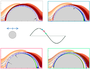
Figure 4. Flow characteristics represented by vorticity contours for cases at (a)  $(K, \beta ) = (0.1, 1035)$, (b) (1.2, 1035), (c) (1.8, 1035) and (d) (2.0, 1035) at a selected instant, where the sampling phase is marked as a red circle filled with black in the sinusoidal velocity signal in the inset of (a).
The increasing deviation of the present DNS results from the S–W solution for  $K > 1.0$ is primarily due to the influence of flow separation, which will be discussed in detail later on. Sarpkaya (Reference Sarpkaya1986) attributed the large deviations of the experimental
  $C_d$ from the S–W solution observed in the case of
  $\beta = 1035$ to the development of 3-D instabilities and the hysteresis effect. We subsequently checked the hysteresis effect through separate DNS tests at
  $\beta = 1035$ and 1380 by gradually increasing and decreasing
  $K$ values and failed to identify a noticeable difference in
  $C_d$ from those DNS with zero initial conditions. The influence of 3-D instabilities on
  $C_d$ will be discussed in the subsection to follow. Since the minimum
  $K (= 0.8)$ value tested was relatively large for the case of
  $\beta = 11\ 240$, the large deviation observed did not attract much attention in Sarpkaya (Reference Sarpkaya1986). We suspect, based on our 2-D and 3-D DNS results, that the large deviation was induced by experimental uncertainties.
3.2. Three-dimensionality
To check the influence of 3-D effect on  $C_d$, a limited number of 3-D DNS are conducted at
  $K$ values that are smaller than the corresponding
  $K$ values on the iso-line of
  $\varLambda _K = 1.5$ with
  $\beta = 200\text {--}20\, 950$. The results from 3-D DNS at
  $\beta$ from 200 to 20 950 are compared with the S–W solution and 2-D DNS results in table 1. The difference between
  $C_d$ values predicted by 3-D and 2-D DNS does increase with increasing
  $K$ and
  $\beta$ values. For instance, the difference increases from 0.50 % to 7.68 % as
  $K$ is increased from 0.8 to 1.4 in the case of
  $\beta = 20\, 950$. For a constant
  $K$ value, e.g.
  $K=1.2$, the difference increases from 0.30 % at
  $\beta = 1035$ to 2.69 % at
  $\beta = 20\, 950$. The present results appear to contradict with previous findings reported in the literature (Nehari, Armenio & Ballio Reference Nehari, Armenio and Ballio2004; Rashid, Vartdal & Grue Reference Rashid, Vartdal and Grue2011) that the 3-D effect does not affect the drag coefficient significantly. This contradiction arises because previous studies were mainly concerned with flows at small
  $\beta$ values, while the large differences between 2-D and 3-D DNS results are observed at either high
  $\beta$ or
  $K$ values in the present study. For the cases with small
  $\varLambda _K$ values investigated in the present study, e.g.
  $\varLambda _K \leq 1.1$, the difference between
  $C_d$ values predicted by 2-D and 3-D DNS is less than 2 %, suggesting 2-D DNS is sufficient for the parameter space bounded by
  $\varLambda _K \leq 1.1$. For this reason, the following discussions are based on 2-D results. Further research efforts are recommended to investigate the potential cause of the significant difference between 2-D and 3-D DNS at large
  $K$ and
  $\beta$ values.
Table 1. Comparisons of  $C_d$ values in the S–W solution, 2-D and quasi-3-D simulations, i.e.
  $\{C_d\}_{\text {S--W}}$,
  $\{C_d\}_{\text {2-D}}$ and
  $\{C_d\}_{\text {3-D}}$ respectively. The values in the brackets behind the
  $\{C_d\}_{\text {3-D}}$ are the relative differences compared with the corresponding 2-D results.

3.3. Flow separation
We speculate that the large  $\varLambda _K$ values are mainly induced by flow separations around the cylinder surface because the S–W solution does not take into account the influence of boundary layer separation on the solution. To examine the influence of flow separation on the
  $\varLambda _K$ values, the spatio-temporal variations of flow separation on the upper surface of the cylinder are first quantified. The separation point is defined as the location where the vorticity on the cylinder surface changes sign and is measured by the separation angle (
 $\alpha _s$) relative to the front stagnation point of the cylinder,
  $(x/D, y/D) = (-0.5, 0)$ (see the inset in figure 5a).

Figure 5. Variations of the instantaneous separation angle ( $\alpha _s$) as a function of phase angle
  $\theta$ at (a)
  $\beta = 1035$ and (b)
  $K = 1$. Corresponding evolutions of free-stream velocity (red solid line) and acceleration (green dashed line) are plotted at the bottom of (b). (c) Evolution of boundary layer separation along the cylinder, represented by streamlines (line with arrows) and vorticity contours, at
  $(K, \beta ) = (1.2, 1035)$. The yellow and red contours represent positive and negative vorticities around the cylinder surface. The streamlines with blue and green colours represent the positive and negative signs of the shear stress.
The influence of  $K$ on the variation of
  $\alpha _s$ with
  $\theta$ is examined for a number of
  $K$ values at
  $\beta = 1035$ in figure 5(a). Corresponding evolutions of free-stream velocity (red solid line) and acceleration (green dashed line) are plotted at the bottom of figure 5(b). For
  $K < 1.0$, the separation initially develops at
  $(x/D, y/D) = (0.5, 0)$ during the deceleration phase of the free-stream velocity (
 $\theta = 90^\circ$–
 $180^\circ$, where
  $\theta = 2{\rm \pi} t/T$ is the phase angle of incoming flow). It then propagates towards the upstream, featured by a decrease of
  $\alpha _s$ with increasing
  $\theta$, and terminates by merging with the upstream separation bubble for
  $\theta > 135^\circ$. The increase of
  $K$ induces an early onset of flow separation and a reduction of propagation rate,
  $\partial \alpha _s/\partial \theta$, in the phase space. For instance, the critical phase angle (
 $\theta _{cr}$) at which separation is initiated equals
  $122^\circ$ at
  $K = 0.4$ and decreases to
  $92^\circ$ at
  $K = 1.0$. A general trend observed in figure 5(a) is that
  $\alpha _s$ decreases almost linearly with
  $\theta$ for
  $\alpha _s > 90^\circ$ and drops sharply for
  $\alpha _s< 90^\circ$. Another flow separation bubble develops from the upstream stagnation point at
  $\theta \approx 135^\circ$, quickly climbs upwards and merges with the separation bubble originated from the downstream. The major flow separation features observed at different
  $\beta$ values with
  $K = 1$ in figure 5(b) are similar to those observed in figure 5(a). The average propagation rate of the separation point along the cylinder surface appears to be less affected by
  $\beta$ than
  $K$. Although
  $\theta _{cr}$ may be sensitive to
  $\beta$, the overall spatio-temporal development patterns of
  $\alpha _s$ at different
  $\beta$ values are similar. For example,
  $\alpha _s$ at
  $\beta =20\,950$ remains near
  $180^\circ$ for
  $70^\circ < \theta < 90^\circ$ before it propagates upstream at a similar rate to those at other
  $\beta$ values. The early occurrence of
  $\theta _{cr}$ in this case has little influence on
  $\varLambda _K$, as shown in figure 2.
The  $\theta _{cr}$ value approaches
  $135^\circ$ at small
  $K$ values, e.g.
  $(K, \beta ) = (0.01, 1035)$ in figure 5(a), with a propagation rate close to infinity. This case can be considered equivalent to no flow separation because the separation point moves from the back stagnation point to the front stagnation point instantly at
  $\theta \sim 135^\circ$, which is identical to the critical phase angle in the Stokes solution of oscillatory flow over a flat plate when the wall shear stress changes sign(Stokes Reference Stokes1851). Furthermore, the leading term of the friction in-line force (
 $F_s$) in the S–W solution by Wang (Reference Wang1968) (see (3.6) in § 3.4) also shows a reversal of skin friction at
  $135^\circ$. This behaviour is expected as the flow with small
  $K$ and large
  $\beta$ is unlikely to feel the curvature effect induced by the cylinder. Since the flow velocity near the cylinder surface is in phase with the shear stress on the cylinder surface and leads the free-stream velocity by
  $45^\circ$, the reversal of the boundary layer flow direction at
  $\theta = 135^\circ$ is responsible for the above flow behaviour. It is worth noting that the point
  $(K, \beta ) = (0.01, 1035)$ is bounded by the
  $\beta = 1/K^2$ line in figure 2, where no flow separation is implied by Wang (Reference Wang1968).
The temporal evolution of flow separations at  $(K, \beta ) = (1.2, 1035)$ is visualised through streamlines near the cylinder surface, as shown in figure 5(c). The blue and green colours of the streamlines represent the positive and negative signs of the shear stress. The red and orange contours represent positive and negative vorticities (
 $\omega _z$) around the cylinder at each phase angle. Although the separation point undergoes substantial development along the circumferential direction on the cylinder surface, the size of the separation bubble in the radial direction is rather limited in this case.
The above observations clearly show that flow separation occurs on the cylinder surface even at very low  $K$ values, as shown in figure 5(a), which is different from the assumption made by Wang (Reference Wang1968). It is the spatio-temporal extent of the flow separation that is dependent on
  $K$ values. For example, the flow separation develops near the end of the deceleration phase of local flow near the cylinder (around
  $\theta = 135^\circ$) and vanishes shortly after the reversal of local flow near the cylinder at
  $K = 0.2$ and 0.4. The onset of flow separation advances forward in the phase space and vanishes at approximately the same phase after the reversal of local flow as
  $K$ is increased. To quantify the influence of
  $K$ on flow separation, a measure for the extent of flow separation over a half-oscillation period is proposed as follows:
 \begin{equation} \varGamma=\frac{1}{{\rm \pi}^2}\Big \{\int_{0}^{\rm \pi}({\rm \pi}-\alpha_s(\theta))\mathrm{d}\theta+\int_{0}^{\rm \pi}\alpha_s^*(\theta)\mathrm{d}\theta\Big \}, \end{equation}
where  $a_s^*$ and
  $a_s$ represent the front and back separation bubbles, respectively;
  $\varGamma$ effectively measures a normalised spatio-temporal extent of flow separation (the shaded area shown in figure 5a) during a half-oscillation period. The results shown in figure 6(a,b) suggest that
  $\varGamma$ increases almost linearly with
  $K$ over a range of
  $\beta$ values and is less sensitive to
  $\beta$. This variation trend of
  $\beta$ with
  $K$ appears to correlate surprisingly well with the variation trend of
  $\varLambda _K$ with
  $K$ shown in figure 2. Correlation between
  $\varGamma$ and
  $\varLambda _K$ over a series of
  $K$ and
  $\beta$ values is plotted in figure 6(c) and can be represented by
 \begin{equation} \varLambda_K \sim 1+101.03\varGamma^{3}. \end{equation}
Figure 6. Variations of the extent of flow separation  $\varGamma$ with respect to (a)
  $K$ and (b)
  $\beta$ values. (c) Correlations between
  $\varGamma$ and
  $\varLambda _K$ for cases shown in (a,b).
The results shown in figure 6(c) suggest that  $\varLambda _K$ correlates extremely well with
  $\varGamma$. The larger the
  $\varGamma$, the more influence it has on
  $\varLambda _K$. The influences of flow separation on pressure and shear stresses on the cylinder surface and hence the drag force are further explored below.
3.4. Time-dependent in-line forces on the cylinder surface
The instantaneous in-line force acting on the cylinder under the oscillatory flow condition ( $U=U_m \sin \theta$) is comprised of three components (Stokes Reference Stokes1851; Wang Reference Wang1968; Bearman et al. Reference Bearman, Downie, Graham and Obasaju1985). The first component is the inviscid inertia force,
  $F_0$, induced by the acceleration of the outer flow, which can be estimated through the potential flow theory as,
 \begin{equation} F_{0}=\frac{{\rm \pi}^2}{K}\rho U_m^2 D \cos \theta.\end{equation}
 The second component considers the contribution of viscous interactions of boundary layers with the cylinder. The viscous boundary layer on the cylinder surface affects the in-line force in two ways (Stokes Reference Stokes1851; Wang Reference Wang1968). The boundary layer profiles determine the distribution of skin friction  $\tau _w$ along the cylinder surface. The shear force,
  $F_s$, can be determined by integrating
  $\tau _w$ along the cylinder surface as
 \begin{equation} F_s = \int_{0}^{2{\rm \pi}} \tau_w \sin \alpha\, \textrm{d}\alpha,\end{equation}
where  $\alpha$ measures the angle from the cylinder surface relative to
  $(x/D, y/D) = (-0.5, 0)$. As the growth of the boundary layer is not uniform over the surface of the cylinder due to the curvature of the body, it induces a perturbation to the pressure distribution around the cylinder surface which subsequently alters the in-line force as well (Stokes Reference Stokes1851; Wang Reference Wang1968). This force is denoted as the viscous force,
  $F_v$, in the present study. In the analytical solution given by Wang (Reference Wang1968),
  $F_s$ and
  $F_v$ are identical and can be calculated as
 \begin{align} F_{v}=F_{s}&=\frac{{\rm \pi}^2}{K}\rho U_m^2 D \left[({\rm \pi}\beta)^{{-}1/2}(\sin \theta+\cos \theta) +({\rm \pi}\beta)^{{-}1}\sin \theta \vphantom{\frac{{\rm \pi}^2}{K}}\right.\nonumber\\ &\quad \left.+\frac{1}{4}({\rm \pi}\beta)^{{-}3/2}(\cos \theta-\sin \theta)\right]. \end{align}
 The third component of the in-line force is induced by extensive separations of viscous boundary layer flow and the generation of vortices (Bearman et al. Reference Bearman, Downie, Graham and Obasaju1985), which modify the distributions of pressure and shear stress around the cylinder. This force is similar to the form drag in steady flow past a stationary cylinder and is denoted as  $F_p$ in the present study. The value of
  $F_p$ becomes significant as
  $K$ exceeds a critical value, depending on
  $\beta$.
Since  $F_v$,
  $F_p$ and
  $F_i$ are determined by the pressure distribution around the cylinder surface, they cannot be separated easily in analysing DNS results. In order to quantify the influence of
  $F_p$ and to compare DNS results of
  $F_v$ with the S–W solution, the following approximations are made to quantify
  $F_v$ and
  $F_p$ in DNS. We assume
  $F_i$ in DNS at low
  $K$ value is identical to the inviscid solution,
  $F_0$ ((3.4)), and the remaining part,
  $F'= \int _{0}^{2{\rm \pi} } p_w \cos \alpha \, \textrm {d}\alpha - F_0$, constitutes an approximation to
  $F_v + F_p$. Here,
  $F'$ is expected to reduce to
  $F_v$ and be identical to
  $F_s$ when the spatio-temporal extent of flow separation is insignificant at small
  $K$ values. The contribution of
  $F_p$ to
  $F'$ will be large when the spatio-temporal extent of flow separation is significant at large
  $K$ values. To validate the above understanding, corresponding variations of
  $\{F_s\}_{DNS}$ and
  $\{ F'\}_{DNS}$, based on DNS results at (
 $K, \beta ) = (0.1, 1035$), (1.4, 1035) and (2.0, 1035), are depicted in figure 7(a–c), together with
  $\{F_s\}_{\text {S--W}}$ based on the S–W solution ((3.6)). The red solid line represents the scaled free-stream velocity. As expected, evolutions of
  $\{F_s\}_{DNS}$ and
  $\{F'\}_{DNS}$ are identical and agree very well with
  $\{F_s\}_{\text {S--W}}$ for the case at (
 $K, \beta ) = (0.1, 1035$) in figure 7(a). The good agreement observed in this case is because the contribution of flow separation is negligible (
 $F_p \sim 0$) at
  $K = 0.1$. The value of
  $F'$ reduces to
  $F_v$ and is identical to the S–W solution ((3.6)). As
  $K$ is increased to 1.4 and 2.0,
  $\{F_s\}_{DNS}$ is slightly larger than
  $\{F_s\}_{\text {S--W}}$. The value of
  $\{F'\}_{DNS}$, on the other hand, deviates significantly from
  $\{F_s\}_{\text {S--W}}$ both in amplitude and phase. The large deviations observed in those two cases are suspected to be primarily due to the
  $F_p$ induced by flow separation. Since
  $F_v = F_s$ based on the S–W solution, the approximation of
  $F'\approx F_v + F_p \approx F_s + F_p$ would allow us to infer the influence of flow separation on
  $F_p$ by quantifying the influence of flow separation on
  $\{F_s\}_{DNS}$ over a half of flow oscillation period, through a measure proposed in the present study:
 \begin{equation} \varPsi=\frac{\displaystyle \int_{0}^{T/2}\{F_s\}_{DNS}\, \textrm{d}t}{\displaystyle \int_{0}^{T/2}\{F_s\}_{\text{S--W}}\, \textrm{d}t}. \end{equation}
The variations of  $\varPsi$ values as a function of
  $K$ at
  $\beta = 1035$ and 20 950 shown in figure 7(d) suggest the spatio-temporal extent of flow separation has little effect on
  $F_{s}$ along the cylinder surface. For instance, flow separation induces only a
  $\varPsi \sim 1.06$ difference on
  $F_s$ at
  $(K, \beta ) = (2.0, 1035)$, whereas the measured
  $C_d$ is around
  $\varLambda _K = 1.43$ times of that by the S–W solution. The large
  $\varLambda _K$ value in this case is clearly caused by the form drag component
  $F_p$.

Figure 7. Time evolutions of  $F_{s}=\int _{0}^{2{\rm \pi} } \tau _w \sin \alpha \, \textrm {d}\alpha$ (orange short-dashed line) and
  $F'= \int _{0}^{2{\rm \pi} } p_w \cos \alpha \, \textrm {d}\alpha - F_0$ (blue dashed line) obtained in terms of DNS results at (a)
  $(K, \beta ) = (0.1, 1035)$, (b) (1.4, 1035) and (c) (2.0, 1035) over one flow oscillation period. The grey solid lines represent the corresponding shear force calculated based on (3.6) in the S–W solution, i.e.
  $\{F_s\}_{\text {S--W}}$. The red solid line represents the scaled free-stream velocity
  $U$. (d) Variations of
  $\varPsi$ values for cases at
  $\beta = 1035$ and 20 950.
3.5. General form of the Morison equation
The validity of the conventional Morison equation (1.1a–c) is questionable under the condition of low  $K$ values where the drag component of
  $F_v+F_s$ dominates the total drag. The first term in (1.1a–c), proportional to
  $U^2$, represents the form drag component
  $F_p$ (Sumer Reference Sumer and Fredsøe1997). The S–W solution shows that
  $F_s+F_v$ is inversely proportional to
  $U$, rather than to
  $U^2$. Based on the results shown in § 3.4,
  $F_s+F_v$ generally dominates the total drag prior to the onset of extensive flow separations on the cylinder surface and
  $F_p$ becomes important after the extent of flow separation increases beyond a certain level. It is plausible to infer that there will be a parameter space where
  $F_s+F_v$ is comparable to
  $F_p$. Since
  $F_s$ is in phase with
  $\partial u_\alpha /\partial r |_{r=0.5}$, where
  $\alpha$ and
  $r$ are the polar coordinates, it contributes to the drag only. The solution of the laminar oscillatory flow above a flat plate shows that
  $\tau _w$,
  $u_\alpha$ and
  $\partial u_\alpha /\partial r |_{r=0.5}$ on the plate lead the free-stream velocity
  $U$ by
  ${\rm \pi} /4$. It is not difficult to deduce from (3.6) and figure 7(a) that this relationship also applies to oscillatory flow around a circular cylinder, where both
  $F_s$ and
  $F_v$ are linearly proportional to
  $U$ with a phase lead of
  ${\rm \pi} /4$.
Based on above reasoning, the use of (1.1a–c) under small  $K$ conditions is fundamentally incorrect because it cannot account for the linearity and phase lead of
  $F_s+F_v$ to
  $U$. Applications of (1.1a–c) will not only lead to an incorrect
  $C_d$ but also poor predictions of time-dependent drag. To rectify the problem, a general form of the Morison equation is proposed in the present study as
 \begin{equation} F_x=\frac{1}{2}\rho D C_{d1}U_m^2\sin(\theta+{\rm \pi}/4)+\frac{1}{2}\rho D C_{d2}U_m^2\sin(\theta)|\sin(\theta)|+\frac{\rm \pi}{4}\rho D^2C_m\frac{\textrm{d}U}{\textrm{d}t}, \end{equation}
where  $U=U_m\sin {\theta }$,
  $C_{d1}$ and
  $C_{d2}$ are the viscous and form drag coefficients, respectively. The first, second and third terms of (3.8) represent
  $F_s + F_v$,
  $F_p$ and
  $F_i$ respectively. The above equation recovers to the conventional Morison equation (1.1a–c) when
  $F_p$ significantly outweighs
  $F_s + F_v$ at large
  $K$ values. Assuming the form drag component is negligible under the applicable condition of the S–W solution, we get the analytical form of
  $C_{d1}$ based on the S–W solution as
  $\{C_{d1}/C_d\}_{\text {S--W}} = 16/(3\sqrt {2}{\rm \pi} ) \approx 1.2$ and the asymptotic form of
  $C_{d1}$ for
  $\beta \gg 1$ reads
  $\{KC_{d1}\sqrt {\beta }\}_{\text {S--W}} \approx 31.49$. This outcome suggests that (1.2) underestimates the peak value of the hydrodynamic damping force by 1.2 times. Since three terms in (3.8) have
  ${\rm \pi} /4$, 0 and
  ${\rm \pi} /2$ phase differences relative to
  $U$, respectively, a specific procedure is needed to determine the hydrodynamic coefficients in (3.8), based on the total in-line force,
  $F_x$, measured in DNS or physical experiments.
The following three options are available to determine the force coefficients in (3.8) based on the numerical results from DNS:
Method I, calculate  $F_s+F_v$ and hence
  $C_{d1}$ based on the S–W solution and determine
  $C_{d2}$ and
  $C_m$ based on (
 $\{F_x\}_{DNS}-\{F_s+F_v\}_{\text {S--W}}$).
Method II, let  $F_s + F_v=2F_s$, estimate
  $F_s$ based on DNS results and determine
  $C_{d2}$ and
  $C_m$ using (
 $\{F_x-2F_s\}_{DNS}$).
Method III, calculate  $C_{d1}$ and
  $C_m$ based on the S–W solution and determine
  $C_{d2}$ based on (
 $\{F_x\}_{DNS}-\{F_s+F_v+F_i\}_{\text {S--W}}$).
The above three methods are expected to be identical at small  $K$ values and yield different results at intermediate
  $K$ values. To evaluate the goodness of fit by using those methods, cases at
  $\beta = 1035$ over a range of
  $K$ values from 0.1 to 8.0 are used to determine a sensible choice of methods I, II and III. Corresponding distributions of
  $C_{d2}$ and
  $C_m$ based on methods I–III, together with those using the conventional Morison equation in (1.1a–c), denoted as method 0 hereafter, are shown in figure 8(a). Figure 8(b) shows the variation of a goodness-of-fit parameter
  $\zeta$ (proposed by Justesen Reference Justesen1989) with
  $K$. The goodness-of-fit parameter
  $\zeta$ is determined based on the measured and predicted phase-averaged drag force over one period
  $T$ as
 \begin{equation} \zeta = \frac{\displaystyle \int_{T}(\{F_d\}_m-\{F_d\}_p)^2\,\textrm{d}t}{\displaystyle\int_{T}\{F_d\}_m^2\,\textrm{d}t}, \end{equation}
where  $\{F_d\}_m$ and
  $\{F_d\}_p$ are the time-dependent measured and predicted drag components. The lower the
  $\zeta$, the better the prediction is. The results suggest that method II yields the best fit and the method 0 leads to the worst fit for
  $K < {\sim }2.0$ at
  $\beta = 1035$. The results by method I are only slightly worse than those by method II at
  $K < {\sim }2.0$. The above results are not totally surprising because method II allows the influence of flow separation to be reflected in all three coefficients, while method I ignores the influence of flow separation on
  $C_{d1}$. Although method I leads to a slightly worse prediction than method II, method I is recommended to quantify
  $C_{d1}$,
  $C_{d2}$ and
  $C_{ m}$ in (3.8) due to the convenience of using the analytical solution of
  $\{C_{d1}\}_{\text {S--W}}$ in the equation.

Figure 8. Distributions of (a)  $C_{d2}$ (solid circles) and
  $C_m$ (solid squares), and (b) goodness-of-fit parameter
  $\zeta$, as a function of
  $K$ at
  $\beta = 1035$ based on DNS results. The red dashed line, blue dotted line, grey solid line and green dash dotted line in (a,b) represent the variations using methods 0–III, respectively.
Reconstructions of temporal variations of the drag force based on (1.1a–c) (method 0) and (3.8) (method I) over one  $T$ at
  $\beta = 1035$ are illustrated in figure 9. Four cases at
  $K = 0.1\text {--}4.0$ are selected to depict the performance of the proposed general form of the Morison equation. By comparing the absolute difference of the measured and predicted drag components, i.e.
  $\{F_d\}_m - \{F_d\}_p$, (3.8) significantly outperforms (1.1a–c) for
  $K < {\sim }2.0$. At small
  $K$, e.g.
  $K = 0.1$ in figure 9(a), the reconstructed drag agrees fairly well with both measured drag values in DNS and the S–W solution (
 $\{F_s+F_v\}_{\text {S--W}}$). Due to the development of the form drag component, the reconstructed drag through method I deviates from the S–W solution as
  $K$ is increased (figure 9 b,c). The general form Morison equation slightly outperforms the conventional one for
  $K > {\sim }2.0$ (figure 9 d), suggesting (3.8) gradually reduces to (1.1a–c) as
  $K$ is increased.

Figure 9. Time evolution of measured drag,  $\{F_d\}_m$, and reconstructed drag,
  $\{F_d\}_p$, at (a)
  $(K, \beta ) = (0.1, 1035)$, (b) (1.4, 1035), (c) (2.0, 1035) and (d) (4.0, 1035) over one period. Corresponding
  $\{F_d\}_m$,
  $\{F_d\}_p$ and
  $\{F_d\}_m - \{F_d\}_p$ obtained through method 0 (red) in (1.1a–c) and method I (blue) in (3.8) are shown as thick solid, dashed and dotted lines.
Variations of  $C_{d1}$ and
  $C_{d2}$ with
  $K$ and
  $\beta$, obtained by using (3.8) through method I, are shown in figure 10(a). As expected, opposite trends of
  $C_{d1}$ and
  $C_{d2}$ are clearly observed as
  $K$ is increased. It is seen in figure 10(a) that
  $C_{d1}$ is approximately 10 times larger than
  $C_{d2}$ for the cases of
  $K < {\sim }1.0$ over a wide range of
  $\beta$, which means the second term on the right-hand side of (3.8) can be ignored. Both
  $C_{d1}$ and
  $C_{d2}$ are equally important at intermediate
  $K$, e.g.
  $0.1< C_{d1}/C_{d2} < 10$ at
  $K= 1.0\text {--}8.0$, where the newly proposed general form of the Morison equation should be utilised. Distributions of
  $\zeta$ with respect to
  $K$ over a range of
  $\beta$ values for method 0 and method I are shown in figure 10(b). The general form of the Morison equation in (3.8) shows an excellent improvement over (1.1a–c) for
  $K < 2.0$. It is also slightly better than (1.1a–c) for
  $2.0 \leq K \leq 8.0$. For large
  $K$ values, e.g.
  $K > 8.0$, above which asymmetry and vortex shedding occur and the in-line force is largely drag dominated (Bearman et al. Reference Bearman, Downie, Graham and Obasaju1985; Sarpkaya Reference Sarpkaya2010), (3.8) recovers to (1.1a–c) where
  $C_{d2}$ is significantly larger than
  $C_{d1}$.

Figure 10. Variations of (a)  $C_{d1}$,
  $C_{d2}$ and (b)
  $\zeta$ as a function of
  $K$ for
  $\beta = 200 - 10^5$. The solid lines with square symbols in (a) are the viscous drag coefficient,
  $C_{d1}$, obtained through the S–W solution, while the triangles indicate the form drag coefficient,
  $C_{d2}$, determined by using method I.
4. Discussion
Previous experimental studies showed controversial results of the measured  $C_d$ values at different
  $\beta$ values. For instance, the physical tests conducted by Sarpkaya (Reference Sarpkaya1986), through U-tube measurements at small
  $\beta \leq 11\ 240$, have shown that the measured
  $C_d$ deviates from the S–W solution after 3-D instabilities develop, leading to a hysteresis effect in the vicinity of the deviation (see grey circles in figure 3a). The potential reasons for the hysteresis are unclear, even now, as this phenomenon has not been observed other than by Sarpkaya (Reference Sarpkaya1986). For cases at
  $\beta > 10^5$, most of the physical tests at low
  $K$ observed that
  $C_d$ was approximately twice
  $\{C_d\}_{\text {S--W}}$ for cases below the
  $K_r$ line (e.g. Chaplin Reference Chaplin2000; Sarpkaya Reference Sarpkaya2001, Reference Sarpkaya2010). We originally hoped that some physical mechanisms would have manifested to allow meaningful explanations for the hysteresis effect at small
  $\beta$ and nearly doubled
  $C_d$ at large
  $\beta$. Unfortunately, both 2-D and 3-D DNS failed to identify any culprit for the large discrepancy. The excellent agreement between the S–W solution and DNS results in the region below the
  $K_r$ line, where the flow is deemed to be two-dimensional and yet large discrepancies between experimental results and the S–W solution exist, appears to suggest that the DNS results are correct and the experimental results are questionable. Since the identification of experimental uncertainties is beyond the scope of the present work, some potential effects are briefly discussed and readers are referred to Sarpkaya (Reference Sarpkaya2001) and Sarpkaya (Reference Sarpkaya2010) for details.
First of all, accurate measurements of  $C_d$ at low
  $K$ values are challenging, because the drag accounts for a very small proportion of the total in-line force. Experimental uncertainties may easily contaminate the drag separated from the total in-line force measured in the experiment. This conjecture is supported by a recent experimental study conducted by Gao et al. (Reference Gao, Efthymiou, Cheng, Zhou, Minguez and Zhao2020) at
  $\beta = 20\,950$, where the measured
  $C_d$ (not shown in this paper) agrees fairly well with both the S–W solution and the present studies at
  $K \sim 1$. Significant deviations from the S–W solution are observed as
  $K$ is decreased in Gao et al. (Reference Gao, Efthymiou, Cheng, Zhou, Minguez and Zhao2020), which contradicts the observations reported in the literature at similar
  $\beta$ (Bearman & Mackwood Reference Bearman and Mackwood1992; Sarpkaya Reference Sarpkaya2006a). Secondly, Sarpkaya (Reference Sarpkaya2001) pointed out that the
  $K_r$ line was only an approximate boundary, depending on uncontrolled conditions in experiments, such as residual background turbulence, undesirable vibrations, nonlinear interaction of various types of perturbations, etc. No attempt is made to quantify the influence of different noises in DNS, since it is not straightforward to examine those effects fully in DNS, based on the current DNS models and computing resources.
We now focus on the appropriateness of the present DNS. An immediate question concerns the possibility that large scale spanwise 3-D structures such as the regime C structure reported by Elston et al. (Reference Elston, Blackburn and Sheridan2006) and Xiong et al. (Reference Xiong, Cheng, Tong and An2018b) exist and were not resolved by the present 3-D DNS. We cannot rule this possibility out because the selection of the computational domain size and mesh resolution in the spanwise direction are based on the empirical characteristic length of the Honji-type 3-D structure ( $\lambda$) reported by Sarpkaya (Reference Sarpkaya2002). The magnitude of
  $\lambda /D$ is O(
 $10^{-3}$) when
  $\beta \sim O(10^6)$. The present use of
  $L_z > 4\lambda$ might not be able to resolve large scale spanwise 3-D structures. The existing knowledge on the flow suggests different 3-D instabilities such as regimes C, D and F often occur at large
  $K$ values that are beyond the parameter range of present DNS. No further attempt was made to address this issue due to the constraint of available computational resources.
No turbulence model is employed in the present study. This choice is primarily made based on an understanding that turbulence is unlikely in the parameter space of present interest. For example, under an assumption of negligible curvature effect, the boundary layer on the cylinder surface in the tests reported by Chaplin (Reference Chaplin2000) at  $\beta = 670\ 000$ with
  $0.001 < K < 0.1$ is deemed to be in the laminar regime based on the existing knowledge of oscillatory flow above a smooth plate. In addition, the independent experience of using turbulence models to simulate the flow has not been very positive. For instance, 3-D large-eddy simulations with a dynamic Smagorinsky model in Rashid et al. (Reference Rashid, Vartdal and Grue2011) showed a large relative difference from experimental results by Sarpkaya (Reference Sarpkaya1986) at large
  $K$, e.g. 28.97 % at
  $(K, \beta ) = (4.86, 1035)$ and 29.3 % at (4, 11 240). The 2-D nonlinear eddy-viscosity model based on the unsteady Reynolds-averaged Navier–Stokes equations conducted by Saghafian et al. (Reference Saghafian, Stansby, Saidi and Apsley2003) showed that
  $C_d$ was overestimated with respect to the S–W solution at small
  $K$, e.g. 17.1 % at
  $(K, \beta ) = (0.5, 1035)$, a point at which both experimental results by Sarpkaya (Reference Sarpkaya1986) and the present results show good agreements with the S–W solution.
5. Conclusions
The applicable bound values of the Keulegan–Carpenter ( $K$) number and Stokes (
 $\beta$) number for the S–W solution (Wang Reference Wang1968), which were given asymptomatically as
  $\beta K^2 \ll 1$ and
  $\beta \gg 1$, are investigated by conducting a series of 2-D and 3-D DNS over
  $K$ from 0.01 to 20 and
  $\beta$ from 1 to
  $10^6$. The S–W solution is found to be applicable over a parameter range that is much larger than the constraints of
  $\beta K^2 \ll 1$ and
  $\beta \gg 1$, based on DNS results. We consider this finding significant as the S–W solution can potentially be used in practical applications over much wider parameter ranges than those suggested by Wang (Reference Wang1968) and the experimental findings reported in the literature. The spanwise structure, such as the Honji instability, which has been speculated as the major cause for the deviation of force coefficients with the S–W solution, is affirmed to have a less effect on the drag and inertia coefficients, i.e.
  $C_d$ and
  $C_m$, at small
  $K$ values. We found that the discrepancy between DNS and the S–W solution, i.e.
  $\varLambda _K$, is mainly associated with the spatio-temporal extent of flow separation on the cylinder surface. Flow separation on the cylinder surface starts from the downstream half of the cylinder surface, propagates towards the upstream half and merges with the front separation bubble over a half of a flow period, relative to the direction of incoming flow. A measure for the spatio-temporal extent of flow separation, i.e.
  $\varGamma$, is introduced to quantify the influence of flow separation, which is more sensitive to
  $K$ than to
  $\beta$. The
  $\varLambda _K$ value is found to correlate extremely well with
  $\varGamma$. The larger the
  $\varGamma$, the larger the
  $\varLambda _K$.
Our results showed that the viscous and form drag components are equally important at intermediate  $K$. On this basis, a general form of the Morison equation is proposed by considering both viscous and form drag coefficients. The viscous drag has a
  ${\rm \pi} /4$ phase difference relative to the incoming flow. In this Morison equation, the linear viscous drag is analytically derived based on the S–W solution. The quadratic form drag and inertia force can be decomposed using the conventional approach based on the remaining parts of the in-line force. The general form of the Morison equation proposed in the present study is demonstrated to be superior to the conventional Morison equation for
  $K < {\sim }2.0$ over a wide range of
  $\beta$ values.
Unfortunately, the present DNS results do not support the experimental findings of a nearly doubled drag force as predicted by the S–W solution at large  $\beta$ and small
  $K$ values. More research efforts on analysing potential experimental errors or exploring potential flow structures that cause the large differences are recommended.
Funding
This work was supported by the National Key R&D Program of China (Project ID: 2016YFE0200100), Natural Science Foundation of China (Grant No. 51779040) and Australia Research Council Discovery Grant (Project ID: DP200102804). The first author would like to acknowledge the financial support from the China Scholarship Council (CSC). This research was supported by computational resources provided by the National Computational Merit Allocation Scheme (NCMAS) and the Pawsey Supercomputing Centre with funding from the Australian Government and the Government of Western Australia.
Declaration of interest
The authors report no conflict of interest.
Appendix A
A.1 Cross-sectional mesh selections
The 2-D mesh convergence check is conducted in the plane perpendicular to the axis of the cylinder. The major tasks in the mesh check include selecting appropriate mesh size and domain size to resolve the flow and minimise the blockage effect. For the mesh type and the computational domain shown in figure 11, we specifically need to select the size of the first layer macro-elements next to the cylinder surface, represented by  ${\rm \Delta} r$ and
  ${\rm \pi} D/N_c$ in the radial and circumferential directions, the total number of macro-elements in the domain
  $N_{el}$, the polynomial order of the macro-element
  $N_p$ and the distances from the centre of cylinder to the boundaries of the rectangular domain
  $L_0$, where
  $N_c$ is the number of macro-elements used to discretise the cylinder surface. The value of
  ${\rm \Delta} r$ is primarily determined by the number of macro-elements needed to resolve the boundary layer around the cylinder. The normalised thickness of the Stokes boundary layer,
  $\delta _{St}/D$, can be estimated by
  $\delta _{St}/D = 2.82\beta ^{-1/2}$ (Sarpkaya Reference Sarpkaya2001). The order of
  $\delta _{St}/D$ is estimated to be from
  $O(0.001)$ to
  $O(1)$ for the
  $\beta$ values investigated in the present study, which is employed to govern the selection of
  ${\rm \Delta} r$. The larger
  $\beta$ is, the smaller the
  ${\rm \Delta} r$ required. In order to save computational costs, the macro-element sizes are gradually changed with increasing distance from the cylinder surface. The expansion ratio of the
  $h$-type mesh near the cylinder surface is set as
  $q_1=1.15$, whereas expansion ratios for the outer domain are set below
  $q_2=1.3$. A parameter
  $N_r=\lfloor \log \{1+(q_1-1)\delta _{St}/{\rm \Delta} r\}/\log q_1\rfloor$, is defined to represent the number of macro-elements required to resolve the Stokes boundary layer.

Figure 11. Computational domain,  $h$-type mesh distribution oscillatory flow past an isolated cylinder at
  $200 < \beta \leq 1035$ (Mesh 1 in table 2). Each element contains
  $N_p^2$ quadrature points, as in the close-up views of
  $hp$-refined meshes (
 $N_p = 5$) around the cylinder in (b,c), where the
  $p$-type mesh is in grey. Velocity boundary conditions are shown in blue boxes. The total element number (
 $N_{el}$) in (a) is 7156;
  $q_1$ and
  $q_2$ in (a) are the expansion ratios near the cylinder and in outer domain, respectively.
Table 2. Influence of the mesh sizes on in-line force coefficients,  $C_d$ and
  $C_m$, at
  $(K, \beta ) = (1.2, 1035)$. Here,
  $N_{el}$ is the total number of macro-elements of the domain;
  $N_p$ is the polynomial order;
  ${\rm \Delta} r$ is the height of the first macro-element next to the cylinder surface;
  $L_o$ is the distance from
  $(x/D, y/D) = (0, 0)$ to the domain boundaries;
  $N_r=\lfloor \log \{1+(q_1-1)\delta _{St}/{\rm \Delta} r\}/\log q_1\rfloor$ represents the number of macro-elements required to resolve the boundary layer. The time-step size
  ${\rm \Delta} t = 0.0005$ is used in this case. The thickness of Stokes boundary layer at
  $\beta = 1035$ equals to
  $\delta _{St}/D = 2.82 \beta ^{-1/2}\sim 0.09$.

In light of the above, different h-type mesh resolutions around the radical and circumferential directions near the cylinder surface for different (K,  $\beta$) parameter ranges are considered in the mesh dependence check. The employment of different 2-D meshes over different
  $K\text {--}\beta$ parameter zones is aimed at minimising the computational costs. To ensure adequate mesh resolutions in the focused parameter space of the present study, i.e. the region from small
  $K$ values to the vicinity of the
  $K_h$ line shown in figure 2, a careful mesh dependence check is conducted at four discrete points at
  $(K, \beta ) = (0.4, 10^6)$, (1, 20 950), (1.2, 1035) and (2, 200), as shown by the diamond symbols in figure 12. The mesh determined at each of those four points is used uniformly in each of the parameter regions governed by the point (the shaded areas with inclined lines in figure 12), e.g. the mesh chosen at
  $(K, \beta ) = (0.4, 10^6)$ is used for all simulations conducted with
  $K \leq 0.4$ and
  $20\,950 < \beta \leq 10^6$ (Case 4 shown in figure 12).

Figure 12. Computational meshes used in different  $K\text {--}\beta$ parameter regions. Diamond symbols indicate four discrete points at (
 $K, \beta ) = (0.4, 10^6$), (1, 20 950), (1.2, 1035) and (2, 200) used for mesh convergence check, as detailed in table 3. Triangular symbols are two cases at
  $(K, \beta ) = (8, 200)$ and (8, 1035) utilised for selecting
  $L_o$ at
  $K > 3$. The grey hollow circles are the 2-D DNS cases conducted in the present study.
The convergence check is first conducted at  $(K, \beta ) = (1.2, 1035)$ to find the correlations between mesh parameters (
 ${\rm \Delta} r$ (
 $N_r$),
  $N_c$,
  $N_p$,
  $N_{el}$ and
  $L_o$) and
  $\beta$, before the convergence checks are conducted at the other three points. The mesh with
  $L_o = 25D$,
  $N_p = 5$,
  ${\rm \Delta} r = 0.001D$ (
 $N_r = 19$) and
  $N_c = 120$ is selected as the reference mesh (see Mesh 1 in table 2). Detailed mesh distributions near the cylinder surface for the reference mesh are shown in figure 11. The following four sets of simulations are conducted with different mesh parameters from those in Mesh 1 to check the influences of the above mesh parameters on
  $C_d$ and
  $C_m$ values:
(i)
$N_p$ is changed to 3 and 7 in Mesh 2 and Mesh 3 respectively;(ii)
${\rm \Delta} r$ is varied from $0.09D$ ($N_r =1$) to $0.0004D$ ($N_r=25$) in Mesh 4 to Mesh 7;(iii)
$N_c$ is changed to 360 and 64 in Mesh 8 and Mesh 9 respectively;(iv)
$L_o$ is increased to $50D$ in Mesh 10.


A mesh with the minimum  $N_{el}$ among the meshes shown in table 2 (Mesh 11), where
  $N_r = 6$ and
  $N_c = 64$, is checked in order to minimise the computational costs for the cases with high
  $\beta$ values. Detailed parameters for each mesh are listed in table 2, together with the
  $C_d$ and
  $C_m$ values based on corresponding meshes. Except for Mesh 7 with
  ${\rm \Delta} r \sim \delta _{St}$ (
 $N_r = 1$), the
  $C_d$ and
  $C_m$ values obtained with different meshes are within
  $1\,\%$ of the corresponding values obtained using the reference mesh. The above results suggest that
  $N_r \ge 6$ and
  $N_c \ge 64$ are adequate to resolve the boundary layer and flow separations. The reference mesh listed in table 2 is more than adequate for the case with
  $K \leq 1.2$ and
  $200 < \beta \leq 1035$.
Similar mesh checks are conducted at  $(K, \beta ) = (0.4, 10^6)$, (1, 20 950) and (2, 200) and the mesh parameters determined through the mesh checks are listed in table 3. The ranges of
  $N_r$ and
  $N_c$ used are identical to those listed in table 2. The corresponding
  $C_d$ and
  $C_m$ are within
  $1\,\%$ difference of the meshes listed in table 3, suggesting the meshes used in the present cases are adequate to obtain accurate results. The time-step size
  ${\rm \Delta} t$ for cases in different parameter ranges varies from
  ${\rm \Delta} t = 10^{-3}$ to
  $10^{-5}$ (table 3), based on the Courant–Friedrichs–Lewy (CFL) stability criterion, which is defined as
 \begin{equation} \textrm{CFL} =\frac{|\boldsymbol{u}|{\rm \Delta} t}{{\rm \Delta} l}, \end{equation}
where  $|\boldsymbol {u}|$ is the magnitude of the velocity in each cell and
  ${\rm \Delta} l$ is the cell size in the direction of the velocity. The maximum value of CFL is kept below 1 for all the simulations conducted in the present study.
Table 3. Computational meshes used in 2-D simulations over  $K\text {--}\beta$ parameter space.

Simulations are extended for  $K$ values beyond the parameter regions governed by those four points in table 3 during the study to (i) provide more data on the variation of
  $\varLambda _K$ as
  $K$ is increased, as introduced in figure 2, and (ii) validate the proposed general form Morison equation in § 3.5. Since numerical results in those regions would not significantly affect the main conclusions drawn in the present study, simulations conducted at points outside those four parameter regions and
  $K \leq 3$ employ one of the meshes determined in table 3 (shaded areas in figure 12). Another group of mesh dependence checks is conducted by increasing
  $L_o$ from
  $25D$ to
  $50D$ for cases at
  $K = 8$ and
  $\beta = 200$ and 1035 (the triangle symbols in figure 12). As a result, the
  $C_d$ values calculated with
  $L_o=25D$ have 5 %–10 % differences compared to the corresponding values obtained using
  $L_o=50D$. Considering the relative difference increases as
  $K$ is increased,
  $L_o = 50D$ is selected for all cases at
  $K>3$ to keep the numerical difference smaller than 5 %. The mesh resolutions around the cylinder surface are consistent with those introduced in table 3.
A.2 Spanwise mesh selections
The spanwise length of the computational domain  $L_z$ and the order of the Fourier expansion
  $N_z$ are the two parameters that need to be determined in the mesh dependence check in the spanwise direction. Previous studies (e.g. An et al. Reference An, Cheng and Zhao2011; Xiong et al. Reference Xiong, Cheng, Tong and An2018a) showed that good correlations exist between
  $L_z$ and the characteristic length of 3-D structures (
 $\lambda$), which can be estimated according to the empirical formula proposed by Sarpkaya (Reference Sarpkaya2002) as,
  $\lambda /D = 22 \beta ^{-3/5}$ (
  $\lambda \sim 0.34D$ at
  $\beta = 1035$). Xiong et al. (Reference Xiong, Cheng, Tong and An2018a) suggested that a ratio of
  $L_z/\lambda \approx 3$ and
  $N_z = 18$ are generally adequate in resolving spanwise structures of oscillatory flows. Since the present computational costs are much higher than those of Xiong et al. (Reference Xiong, Cheng, Tong and An2018a) and An et al. (Reference An, Cheng and Zhao2011) due to the large
  $\beta$ values involved, a mesh dependence check is conducted again to explore the possibilities of reducing the
  $L_z$ and
  $N_z$ values recommended by Xiong et al. (Reference Xiong, Cheng, Tong and An2018a). For this purpose, the convergence test was initially conducted at (
 $K, \beta ) = (1.2, 1035$).
The reference mesh uses an identical cross-sectional mesh to that employed in the 2-D mesh dependence check with  $L_z = 2D$ and
  $N_z = 64$. The values
  $L_z/\lambda \approx 3 - 12$ and
  $N_z = 32 - 128$, as detailed in table 4, are employed to examine the influence of different combinations of
  $L_z$ and
  $N_z$ on the numerical results. Specifically,
  $L_z$ is varied from
  $1D({\sim } 3 \lambda )$ to
  $4D(\sim 12 \lambda )$ with
  $\lfloor \lambda /{\rm \Delta} z\rfloor = 10$ in Cases 2-2 and 2-3 and
  $L_z = 2D$ and
  $N_z = 32 - 128$ in Cases 2-4 and 2-5, where
  ${\rm \Delta} z = L_z/N_z$ represents the thickness of the spanwise mesh. The
  $C_d$ and
  $C_m$ results shown in table 4 demonstrate that use of
  $\lfloor \lambda /{\rm \Delta} z \rfloor = 5$ leads to a large relative error of
  $C_d$ approximately 2.0 % in Case 2-4 and all other options, including the
  $L_z= 1D$ and
  $N_z = 32$ in Case 2-2, lead to a relative error of
  $C_d$ less than
  $0.03\,\%$ of the corresponding values obtained using the reference mesh. Therefore the parameters chosen for the reference mesh are considered adequate for the case of (
 $K, \beta ) = (1.2, 1035$).
Table 4. Comparisons of 3-D simulation results for  $C_d$ and
  $C_m$ with previous experimental and numerical studies at
  $(K, \beta ) = (2, 200)$ and (1.2, 1035). Here,
  $L_z$ is the spanwise length used in quasi-3-D simulations;
  $N_z$ represents spanwise resolution and
  ${\rm \Delta} z=L_z/N_z$. The characteristic length of the Honji-type instability
  $\lambda /D = 22\beta ^{-3/5}$ at
  $\beta = 200$ and 1035 is equal to
  ${\sim }0.92$ and 0.34, respectively.

Based on the above results, a conservative choice of  $L_z \ge 4\lambda$ and
  $N_z = 64$ is made for different (
 $K$,
$K$,  $\beta$) ranges to allow a wider spectrum to be included. The mesh parameters used in the present quasi-3-D simulations are listed in table 5. Comparisons of
  $C_d$ and
  $C_m$ at (
 $K, \beta ) = (2, 200$) with numerical results in Xiong et al. (Reference Xiong, Cheng, Tong and An2018a) are offered in table 4, suggesting the selections of
  $L_z$ and
  $N_z$ are sufficient.
Table 5. Computational meshes used in quasi-3-D simulations.


