2.1. The long-wave limit

In the limit $\epsilon = 1/W \to 0$, we write

(2.11)\begin{equation} \psi(X,y,T) = \psi^{0} + \epsilon^{2} \psi^{1} + O(\epsilon^{3}) \ldots, \end{equation}

where we have introduced the long-wave co-ordinate $X = x/W$ and slow time $T = t/W$. At leading order in $\epsilon$, the field equation (2.10) becomes

(2.12)\begin{equation} \frac{\partial^{2} {\psi^{0}}}{\partial {y}^{2}} - \psi^{0} + a^{2} \left(\mathcal{H}(Y_h - y) - \mathcal{H}(Y - y)\right) = 0. \end{equation}

The solution to (2.12) depends on whether the PV front is on the shelf ($Y < Y_h$) or off the shelf ($Y > Y_h$). For the case where the front is on the shelf,

(2.13) \begin{equation} \psi^{0}(X,y,T) = \begin{cases} Q\, \mathrm{e}^{{-}y} + a^{2} \sinh{(y)} ( \mathrm{e}^{{-}Y} - \mathrm{e}^{{-}Y_h}), & 0 < y < Y, \\ Q\, \mathrm{e}^{{-}y} +a^{2} [1 - \sinh{(y)} \,\mathrm{e}^{{-}Y_h} - \cosh{(Y)}\, \mathrm{e}^{{-}y}], & Y < y < Y_h, \\ Q\, \mathrm{e}^{{-}y} + a^{2} \left( \cosh{(Y_h)} - \cosh{(Y)} \right)\mathrm{e}^{{-}y} , & y > Y_h, \end{cases} \end{equation}

while when the front is off the shelf,

(2.14) \begin{equation} \psi^{0}(X,y,T) = \begin{cases} Q \,\mathrm{e}^{{-}y} + a^{2} \sinh{(y)} (\mathrm{e}^{{-}Y} - \mathrm{e}^{{-}Y_h}), & 0 < y < Y_h, \\ Q \,\mathrm{e}^{{-}y} + a^{2}[{-}1 + \sinh{(y)} \mathrm{e}^{{-}Y} + \cosh{(Y_h)} \,\mathrm{e}^{{-}y}], & Y_h < y < Y, \\ Q \,\mathrm{e}^{{-}y} + a^{2} ( \cosh{(Y_h)} - \cosh{(Y)})\mathrm{e}^{{-}y}, & y > Y, \end{cases} \end{equation}

upon enforcing continuity of $\psi$ and $u$ at $y = Y$ and $Y = Y_h$ as well as the boundary conditions (2.8). We introduce the index $j = \operatorname {sign}{(Y_h - Y)}$ to differentiate between the two cases, and write

(2.15) \begin{align} \psi^{0}(X,Y,T) &= Q \,\mathrm{e}^{{-}Y} + \frac{a^{2}}{2} [\mathrm{e}^{-(Y + Y_h)} - \mathrm{e}^{{-}2Y} + j (1 - \mathrm{e}^{j(Y - Y_h)} ) ] \nonumber\\ &= Q_e(Y, Y_h). \end{align}

The function $Q_e(Y,Y_h)$ depends on $X$ only through location of the PV interface $Y$ and the shelf width $Y_h$, and, thus, is the hydraulic functional for this problem (Gill Reference Gill1977; Pratt & Whitehead Reference Pratt and Whitehead2008). The net along-shore flux of shelf water is given by $Q - Q_e$. Substituting (2.15) into the kinematic boundary condition (2.7), we have

(2.16)\begin{equation} \frac{\partial {Y}}{\partial {T}} + C(Y, Y_h) \frac{\partial {Y}}{\partial {X}} = \frac{a^{2}}{2} (\mathrm{e}^{j(Y - Y_h)} - \mathrm{e}^{-(Y + Y_h)}) \frac{\partial {Y_h}}{\partial {X}}, \end{equation}

which is a forced nonlinear wave equation with long-wave speed

(2.17)\begin{equation} C(Y, Y_h) ={-} \frac{\partial {\psi^{0}}}{\partial {y}}\rvert_{y = Y} = Q\,\mathrm{e}^{{-}Y} + \frac{a^{2}}{2} [\mathrm{e}^{-(Y + Y_h)} - 2 \,\mathrm{e}^{{-}2Y} + \mathrm{e}^{j(Y - Y_h)}]. \end{equation}

Equation (2.16) will be referred to as the hydraulic equation. From left to right, the terms in (2.17) can be identified as the contributions from: background flow, image vorticity due the shelfbreak, image vorticity due to the PV front, and stretching/squashing generated by off- or on-shelf movement of the front. Much of the qualitative behaviour of the hydraulic equation can be understood through $C$. In particular, if $Y > Y_h$ then $C$ is not a monotonic function of $Y$, but rather has a unique maximum at

(2.18)\begin{equation} Y = Y_2 ={-} \log{\left( \frac{Q + a^{2} \cosh{(Y_h)}}{2 a^{2}} \right)}. \end{equation}

Thus, in the language of conservation laws, the flux function $Q_e$ may be non-convex when the front is off-shelf. Non-convex flux functions admit a rich variety of compound-wave solutions, and are studied in detail for the canonical example of the Riemann problem (i.e. the initial-value problem where the initial condition is a step change in $Y$) by El, Hoefer & Shearer (Reference El, Hoefer and Shearer2017) for the modified Korteweg–de Vries equation, and by JJ20 for the present model without a shelf. Note that (2.18) is valid (i.e. $Y_2 > Y_h$) only when $Q < a^{2}$ and

(2.19)\begin{equation} Y_h < {Y}_{{{2,M}}} = \log{\left(\frac{\sqrt{(1 + 3a^{4})} - Q}{a^{2}}\right)}. \end{equation}

Thus, when $Q = 1$ and the background current is in the same direction as CTW phase propagation, compound-wave structures exist when the flow is dominated by vorticity ($a > 1$), as in JJ20. However, when $Q = -1$ and the background current opposes CTW propagation, compound-wave structures exist for all $a$, provided the shelfbreak $Y_h$ is sufficiently close to the coast (i.e. $Y_h < {Y}_{{{2,M}}}$). Note also that $\partial C/ \partial Y$ is discontinuous at the shelfbreak and, for the case where $Q = -1$, changes sign if $Y_h > {Y}_{{{2,M}}}$. Thus, compound-wave solutions can also occur in the Riemann problem when the front crosses the shelfbreak; although this situation does not arise in the initial-value problem (2.4).

2.2. Dispersive effects

At next order in $\epsilon = 1/W$, the streamfunction correction $\psi ^{1}(X,y,T)$ satisfies

(2.20)\begin{equation} \frac{\partial^{2} {\psi^{1}}}{\partial {y}^{2}} - \psi^{1} ={-}\frac{\partial^{2} {\psi^{0}}}{\partial {X}^{2}}. \end{equation}

Although formally the power series expansion in $\epsilon$ requires that $W \gg {L}_{{{R}}}$, we show in § 5 that the first-order dispersive correction $\psi ^{1}$ captures the qualitative (and much of the quantitative) behaviour of the full QG system even when $\epsilon = 1$ and, thus, $W = {L}_{{{R}}}$. This is also true in JJ20 and in long-wave models of coastal outflows (Johnson et al. Reference Johnson, Southwick and McDonald2017). Equation (2.20) is to be solved subject to continuity of $\psi ^{1}$ and $u^{1}$ at $Y$ and $Y_h$, and the coastal boundary condition $\psi ^{1}(X,0,T) = 0$. After some algebra, we find that

(2.21)\begin{align} \psi^{1}(X,Y,T) &={-}\frac{a^{2}}{4} \frac{\partial^{2} {Y}}{\partial {X}^{2}} + \frac{a^{2}}{4} \mathrm{e}^{{-}2Y} \left(\frac{\partial^{2} {Y}}{\partial {X}^{2}} - 2 Y \left(\frac{\partial {Y}}{\partial {X}}^{2} - \frac{\partial^{2} {Y}}{\partial {X}^{2}} \right) \right) \nonumber\\ &\quad + \frac{a^{2}}{4} \mathrm{e}^{-(Y + Y_h)} \left( Y \left(\frac{\mathrm{d} {Y_h}}{\mathrm{d} {X}}^{2} - \frac{\mathrm{d}^{2} {Y_h}}{\mathrm{d} {X}^{2}} \right) + Y_h \frac{\mathrm{d} {Y_h}}{\mathrm{d} {X}}^{2} - \frac{\mathrm{d}^{2} {Y_h}}{\mathrm{d} {X}^{2}}(1 + Y_h) \right) \nonumber\\ &\quad + \frac{a^{2}}{4} \mathrm{e}^{j(Y-Y_h)} \left( Y \left(\frac{\mathrm{d} {Y_h}}{\mathrm{d} {X}}^{2} -j \frac{\mathrm{d}^{2} {Y_h}}{\mathrm{d} {X}^{2}} \right) - Y_h \frac{\mathrm{d} {Y_h}}{\mathrm{d} {X}}^{2} + \frac{\mathrm{d}^{2} {Y_h}}{\mathrm{d} {X}^{2}}(1 + j Y_h) \right). \end{align}

Substituting (2.21) into the kinematic boundary condition (2.7) gives the dispersive long-wave equation

(2.22)\begin{equation} \frac{\partial {Y}}{\partial {T}} + (C + \epsilon^{2} C^{1}) \frac{\partial {Y}}{\partial {X}} = \frac{\partial {~}}{\partial {X}} (\psi^{0}(X,Y,T) + \epsilon^{2} \psi^{1}(X,Y,T)), \end{equation}

where $C^{1} = - \partial \psi ^{1} / \partial Y$ can be computed from (2.21) using

(2.23a,b)\begin{equation} \frac{\mathrm{d} {~}}{\mathrm{d} {Y}} \left(\frac{\partial^{2} {Y}}{\partial {X}^{2}} \right) = \left.\frac{\partial^{3} {Y}}{\partial {X}^{3}} \right/ \frac{\partial {Y}}{\partial {X}}, \quad \frac{\mathrm{d} {~}}{\mathrm{d} {Y}} \left(\frac{\partial {Y}}{\partial {X}}\right)^{2} = 2 \frac{\partial^{2} {Y}}{\partial {X}^{2}}. \end{equation}

Note that outside the region of topographic forcing, $Y_h$ is constant and (2.21) and (2.22) revert to equations (2.17) and (2.18) in JJ20. An additional conservation law, which is needed for the dispersive shock-fitting applied below, may be formed by multiplying (2.22) through by $Y$,

(2.24) \begin{align} &\frac{\partial {~}}{\partial {T}} Y^{2} + \frac{\partial {~}}{\partial {x}}[2 Q(Y+1)\,\mathrm{e}^{{-}Y}] \nonumber\\ &\qquad \,\, + a^{2} \frac{\partial {~}}{\partial {X}} \left[ (Y+1)\,\mathrm{e}^{-(Y + Y_h)} - \left(Y + \frac{1}{2}\right) \mathrm{e}^{{-}2Y} +(1 - j Y)\,\mathrm{e}^{j(Y - Y_h)} \right] \nonumber\\ &\qquad \,\, + a^{2} \epsilon^{2} \frac{\partial {~}}{\partial {X}} \left[Y^{2} \frac{\partial {Y}}{\partial {X}}^{2} \,\mathrm{e}^{{-}2Y} + \frac{1}{4}\left(\frac{\partial {Y}}{\partial {X}}^{2} - 2 Y \frac{\partial^{2} {Y}}{\partial {X}^{2}} \right)({-}1 + (1 + 2Y)\,\mathrm{e}^{{-}2Y}) \right]\nonumber\\ &\qquad \,\, = 0. \end{align}

3.1. Steady solutions

By the kinematic boundary condition (2.7), $\psi$ is constant in steady flow. In the hydraulic equation this requires that

(3.1)\begin{equation} Q_e(Y, Y_h) = \varPhi \end{equation}

for some constant $\varPhi$, with $Q_e$ the hydraulic functional defined in (2.15). Contours of $Q_e$ for the particular choice of parameters $Q = -1$ (i.e. background flow opposing CTW propagation) and $a = 0.8795$ are shown in figure 3(a). Given a shelfbreak profile $Y_h$ (in fact, given just the far-field width ${Y}_{{{0}}}$ and the perturbation magnitude $\varDelta$), each contour in figure 3(a) that crosses $Y_h = {Y}_{{{0}}}$ and $Y_h = {Y}_{{{0}}} - \varDelta$ represents a possible steady solution $Y$ to the hydraulic equation (2.16). The steady solution chosen by the initial-value problem can be determined as follows.

Figure 3. (a) Contours of the hydraulic function $Q_e(Y,Y_h)$. Steady solutions must lie on a single contour. The black dashed lines are $Y = Y_h$ and $Y_h = 1$, and dotted lines show critical values of the perturbation size $\varDelta$ at which the solution changes type when ${Y}_{{{0}}} = 1$. The red dashed curves show examples of supercritical and critically controlled solutions which are plotted as the solid lines in (b,c), respectively, and the shelfbreak $Y_h(x)$ is shown dashed. The non-dimensional Rossby radius is $a = 0.8795$ and $Q = -1$ so that the background flow opposes Rossby wave propagation, with $\varDelta = 0.01$ in (b) and $\varDelta = 0.05$ in (c).

For small $\varDelta < {\varDelta }_{{{cr}}}$, the flow evolves to become steady in the forcing region, and the steady state is entirely subcritical or supercritical. Transient disturbances thus propagate away from the forcing region in one direction only and the initial condition $Y = {Y}_{{{0}}}$ persists on the other side. Thus, the constant $\varPhi$ may be determined by evaluating (3.1) on the undisturbed side,

(3.2)\begin{equation} \varPhi = Q_e({Y}_{{{0}}}, {Y}_{{{0}}}) ={-} \mathrm{e}^{-{Y}_{{{0}}}}. \end{equation}

Figure 3(b) shows an example of steady supercritical flow when ${Y}_{{{0}}} = 1$ and $\varDelta = 0.01$. The solid curve is the PV front $Y$ and the dashed curve is the shelfbreak $Y_h$, and in order to see the scale of the topographic forcing region this and all other solutions have been plotted in the original co-ordinate $x$. The long-wave co-ordinate $X = x/W$ is found by rescaling the horizontal axis so that the topographic perturbation lies in $|X| < 1$. The contour corresponding to figure 3(b) is highlighted in (a) (upper red dashed curve). The solution starts at $(Y, Y_h) = (1,1)$ and follows the contour (3.2) to the maximum perturbation $Y_h = 0.99$ as the shelf narrows, before retracing the path to $(1,1)$ as the shelf widens again. The solution is therefore symmetric about the origin and the front is off-shelf ($Y > Y_h$) throughout.

If $\varDelta > {\varDelta }_{{{cr}}}$ is sufficiently large then the contour through $({Y}_{{{0}}}, {Y}_{{{0}}})$ does not extend to the maximum displacement $Y_h = {Y}_{{{0}}} - \varDelta$, and instead the steady solution selects the unique contour that satisfies

(3.3)\begin{equation} C(Y,{Y}_{{{0}}} - \varDelta) = 0. \end{equation}

The long-wave speed vanishes at the maximum topographic displacement, which is thus a control point for the flow (Pratt & Whitehead Reference Pratt and Whitehead2008). The vanishing long-wave speed corresponds to a turning point in the $(Y, Y_h)$-plane, so that the contour selected by the initial-value problem in a critically controlled flow is the one that is horizontal at $Y_h = {Y}_{{{0}}} - \varDelta$. Given a far-field shelf width ${Y}_{{{0}}}$, the critical value ${\varDelta }_{{{cr}}}$ beyond which the flow becomes controlled is thus that at which the contour through $({Y}_{{{0}}}, {Y}_{{{0}}})$ is horizontal (${\varDelta }_{{{cr}}}$ is shown for ${Y}_{{{0}}} = 1$ as a dotted line in figure 3a). Figure 3(c) shows an example of a critically controlled flow with $\varDelta = 0.05$, and the corresponding contour is highlighted in (a) (lower red contour). The solution traces the highlighted section of the contour once, so that $Y$ is monotonic and asymmetric as a function of $Y_h$. Note that $Y \neq {Y}_{{{0}}}$ when $Y_h = {Y}_{{{0}}}$ so that a critically controlled flow alters the far-field state on both sides of the shelfbreak perturbation. Note also that the PV front upstream of the perturbation (relative to the background current, $x > 0$) has been displaced far into the open ocean, so that the critically controlled flow is associated with enhanced shelf–open-ocean exchange.

To determine the conditions that lead to critical flow, first consider an asymptotic expansion of the long-wave speed $C(Y, Y_h)$ about the far-field state $Y = Y_h = {Y}_{{{0}}}$. To leading order,

(3.4)\begin{equation} C \sim Q \,\mathrm{e}^{-{Y}_{{{0}}}} - \frac{a^{2}}{2} \mathrm{e}^{{-}2 {Y}_{{{0}}}} + \frac{a^{2}}{2}. \end{equation}

The right-hand side of (3.4) vanishes when $F = 1$, where

(3.5)\begin{equation} F = \frac{- Q}{a^{2} \sinh{({Y}_{{{0}}})}} \end{equation}

is the Froude number for this problem. The condition $F = 1$ can only be satisfied if $Q = -1$ and, thus, as in ZL17, hydraulic control is only possible when the background current opposes CTW propagation. One can also show that control only occurs when the perturbation is a localised narrowing in shelf width ($\varDelta > 0$) as follows. In order for disturbances to propagate away from the forcing region, the critically controlled solution must have $C > 0$ for large positive $X$ and $C < 0$ for large negative $X$. Since $C$ is dominated by the term due to the front moving on or off the shelf, we can conclude that $Y > Y_h$ for large positive $X$ (vortex stretching generates $C > 0$) and $Y < Y_h$ for large negative $X$, so that $\partial Y / \partial X > 0$ in controlled flow. Writing the steady version of (2.16) as

(3.6)\begin{equation} C(Y,Y_h) \frac{\partial {Y}}{\partial {X}} = \frac{\mathrm{d} {Y_h}}{\mathrm{d} {X}} \frac{\partial {Q_e}}{\partial {Y_h}}, \end{equation}

where $\partial Q_e / \partial Y_h > 0$, we see that in a critically controlled flow $C$ and $\mathrm {d} Y_h / \mathrm {d} X$ have the same sign. That is, $\mathrm {d} Y_h/\mathrm {d} X > 0$ for $X$ positive and the perturbation must be a local decrease in shelf width. From now on we will restrict our attention to $\varDelta > 0$ and $Q = -1$ and, thus, describe $x > 0$ as ‘upstream’ relative to the background flow. Critically controlled flows are subcritical ($C > 0$, $F < 1$) upstream of the shelfbreak perturbation and supercritical ($C < 0$, $F > 1$) downstream. In completely supercritical flow $C < 0$ everywhere, $\mathrm {d} Y_h / \mathrm {d} X$ and $\partial Y / \partial X$ have opposite signs and the front is displaced off the shelf (figure 3b), while in subcritical flow the front is on the shelf. Haynes et al. (Reference Haynes, Johnson and Hurst1993) and Johnson & Clarke (Reference Johnson and Clarke1999) study the related problem of a hydraulically controlled flow in a stepped channel, and show that several other types of controlled solutions can occur. The fact that these do not appear in the present geometry suggests that they rely on an opposing wall to support their existence, as can be deduced by figure 2 of Johnson & Clarke (Reference Johnson and Clarke1999).

3.2. Offshore plumes

Assuming that the front is off-shelf at the control point, solving the criticality condition (3.3) gives

(3.7)\begin{equation} Y ={-}\log{\left(\frac{-1}{a^{2}} + \cosh{({Y}_{{{0}}} - \varDelta)}\right)}. \end{equation}

This is the locus of turning points in the hydraulic contours of figure 3(a). As $\varDelta \to \varDelta _0 = {Y}_{{{0}}} - \textrm {acosh}{(1/a^{2})}$, the control point $Y \to \infty$ and the critical solution is no longer valid. The lower dotted line in figure 3(a) gives $\varDelta _0$ when ${Y}_{{{0}}} = 1$. For $\varDelta > \varDelta _0$, neither the supercritical nor critically controlled solution exists and the flow never becomes steady. Instead, the flow develops into an ever-expanding ‘offshore plume’ similar to the growing solutions for coastal outflow plumes discussed in Johnson et al. (Reference Johnson, Southwick and McDonald2017) and Jamshidi & Johnson (Reference Jamshidi and Johnson2019). As in Johnson et al. (Reference Johnson, Southwick and McDonald2017), offshore plumes only exist when $a < 1$ and the flow induced by vortex stretching as shelf water crosses the shelfbreak is not sufficient to overcome the background current. Instead, the incoming flow is directed principally off shore, and $Y$ grows indefinitely in the forcing region. Offshore plumes have no equivalent in free-surface hydraulic flow, which always becomes steady, but are somewhat related to the ‘supercritical leap’ of Haynes et al. (Reference Haynes, Johnson and Hurst1993) in that the flow attains two different supercritical states on either side of the topographic forcing region.

Numerical simulations of (2.16) show that at large times the shape of the front in the source region is approximately constant so that $\partial Y/ \partial T$ is independent of $X$. Thus, we can obtain an approximate description of the offshore plume through the ansatz

(3.8)\begin{equation} Y(X,T) = Y_p(X) + g(T). \end{equation}

Ignoring terms proportional to $\exp {(-2Y)}$ in (2.16) and only considering regions where $Y > Y_h$, we have

(3.9)\begin{equation} \frac{\partial {Y}}{\partial {T}} = \left[(1- a^{2} \cosh{(Y_h)})\frac{\partial {Y}}{\partial {X}} + a^{2} \sinh{(Y_h)} \frac{\mathrm{d} {Y_h}}{\mathrm{d} {X}} \right] \mathrm{e}^{{-}Y}. \end{equation}

Substituting (3.8) into (3.9) gives the separable equation

(3.10)\begin{equation} \mathrm{e}^{g(T)}\frac{\mathrm{d} {g}}{\mathrm{d} {T}} = \left[(1 - a^{2}\cosh{(Y_h)})\frac{\mathrm{d} {Y_p}}{\mathrm{d} {X}} + a^{2} \sinh{(Y_h)}\frac{\mathrm{d} {Y_h}}{\mathrm{d} {X}}\right]\mathrm{e}^{{-}Y_p(X)}, \end{equation}

where the left-hand side is a function of $T$ alone and the right-hand side is a function of $X$ and so both are equal to $\beta$, a constant. Solving each side separately we find that

(3.11a)\begin{equation} g(T) = \log{(T - T_0)} + \log{\beta}, \end{equation}

and, via the substitution $\exp {(Y_p)} = \theta (X)(-1 + a^{2} \cosh {(Y_h)})$ for $\theta (X)$ unknown,

(3.11b)\begin{equation} Y_p(X) = \log{[({-}1 + a^{2} \cosh{(Y_h)})/(X - X_0)]} - \log{\beta}, \end{equation}

so that, at late times in the offshore plume,

(3.12)\begin{equation} Y(X,T) \approx \log{[({-}1 + a^{2} \cosh{(Y_h)})(T - T_0)/(X - X_0)]} \end{equation}

for some constants $T_0$ and $X_0$. Note that the numerator is an even function of $X$ so that in general (3.12) has two singularities. If $X_0 > 0$ is chosen so that $\cosh {[Y_h(X_0)]} = 1/a^{2}$, the singularity at $X = X_0$ may be eliminated. Equation (3.12) is then valid in $X > -X_0$, while for $X < -X_0$, the asymptotic solution approaches the unique contour that has its control point at $Y_h = \varDelta _0$, $Y \to \infty$. The combined asymptotic solution is singular at $X = -X_0$.

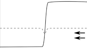
Figure 4 shows instantaneous streamfunction contours in a numerical simulation of the initial-value problem (2.16) in the offshore plume regime. The contours are shown dash–dotted, and the thick black curve is the plume boundary $Y$. There is a slow, broad recirculation of shelf water in the region of topographic forcing and upstream, and the plume boundary at $t = 15\, 000$ agrees well with the asymptotic solution (red dashed curve) away from the singularity at $x = -x_0$ (the black dotted line). The flow upstream is undisturbed and the along-shore flux of shelf water is $1 - \exp {(-{Y}_{{{0}}})}$ while the downstream flux is $1 - a^{2}/2$, which is the asymptotic value of $Q_e$ as $Y \to \infty$.

Figure 4. Offshore plume solution to the hydraulic initial-value problem (2.16). Dash–dot curves show contours of the streamfunction $\psi ^{0}$ at $t = 15\,000$ (contour interval is 0.15), the thick black curve is the frontal position $Y$, the red dashed curve is the asymptotic solution (3.12) and the black dashed curve is the topography $Y_h(x)$. The black dotted line is $x = -x_0$, the location of the singularity in the asymptotic solution. Parameters are ${Y}_{{{0}}} = 0.8$, $\varDelta = 0.7$, $a = 0.9895$ and $W = 5$.

3.3. Boundaries for critical control

An alternative approach to the hydraulic diagram of figure 3 is to consider the problem in the $(\varDelta , F)$-plane. Given the far-field shelf width ${Y}_{{{0}}}$, we seek the range of Froude numbers,

(3.13)\begin{equation} F_-(\varDelta) < F < {F}_{{{+}}} (\varDelta), \end{equation}

for which critical flow occurs. The curves $F_{\pm }$ mark the transition from critical to non-critical flow, and are derived analytically in Appendix A by simultaneously solving the criticality condition (3.3) and the condition for steady, non-critical flow (3.2). These boundaries can also be expressed in terms of the parameter $a$. Figure 5(a) shows how the $(\varDelta , F)$-plane is divided for a narrow shelf (${Y}_{{{0}}} = 0.5$). The flow is supercritical for $F > {F}_{{{+}}}$ and subcritical for $F < {F}_{{{-}}}$. For wider shelves (figure 5(b), ${Y}_{{{0}}} = 1$), the curve ${F}_{{{+}}}(\varDelta )$ is non-monotonic and offshore plumes occur in the region marked ‘growing’, where $F$ lies between ${F}_{{{G}}}(\varDelta )$ (shown dashed) and ${F}_{{{max}}}$, the maximum value of ${F}_{{{+}}}$ and also the point of intersection between the two curves.

Figure 5. Regions of the $(\varDelta , F)$-plane where the flow is critically controlled. (a) A narrow shelf, here with ${Y}_{{{0}}} = 0.5$. The flow is critically controlled when $F$ lies between the solid curves $F_{\pm }(\varDelta )$. (b) A wide shelf, here with ${Y}_{{{0}}} = 1$. The dashed curve is ${F}_{{{G}}}(\varDelta )$, and offshore plumes occur when ${F}_{{{G}}} < F < {F}_{{{max}}}$.

3.4. Transition to the far-field solution

Outside the region of topographic forcing, the hydraulically controlled flow displaces the PV front $Y$ from its initial position ${Y}_{{{0}}}$ to a new, constant, location that we denote ${Y}_{{{u/d}}}$ for $x > 0$ and $x < 0$, respectively. By the heuristic arguments of § 3.1 we expect that controlled solutions are off-shelf upstream and on-shelf downstream, so that ${Y}_{{{u}}} > {Y}_{{{0}}}$ and ${Y}_{{{d}}} < {Y}_{{{0}}}$. If the flow is off-shelf controlled then

(3.14)\begin{align} \mathrm{e}^{-{Y}_{{{u}}}} &={-}\frac{1}{a^{2}} + \cosh{({Y}_{{{0}}})} \nonumber\\ &\quad - \left[(\cosh{({Y}_{{{0}}})} - \cosh{({Y}_{{{0}}} - \varDelta)}) \left(\cosh{({Y}_{{{0}}})} + \cosh{({Y}_{{{0}}} - \varDelta)} - \frac{2}{a^{2}} \right) \right]^{1/2}. \end{align}

To obtain ${Y}_{{{u}}}$ in on-shelf controlled flow, or ${Y}_{{{d}}}$ in either case, requires the solution of at least one cubic equation and yields an expression that is too complex to include here. The dependence of ${Y}_{{{u/d}}}$ on $F$ and $\varDelta$, for the case where ${Y}_{{{0}}} = 0.8$, is shown in figure 6. Increasing $F$ moves the front offshore both downstream and upstream of the topographic perturbation, while increasing $\varDelta$ leads to a more extreme displacement of the front relative to the shelfbreak (further offshore upstream, further onshore downstream).

Figure 6. Adjusted frontal position in controlled flow (a) downstream and (b) upstream of the topographic perturbation, for ${Y}_{{{0}}} = 0.8$ and various values of Froude number $F$ and topographic perturbation magnitude $\varDelta$. Shown are the analytic solutions (curves) and numerical solutions to the dispersive long-wave equation (symbols). The solid curves and circles are for shelves with $\varDelta = 0.05$, dashed curves and squares with $\varDelta = 0.1$ and dash–dot curves and triangles with $\varDelta = 0.25$.

The transition between the topographically influenced state ${Y}_{{{u/d}}}$ and the undisturbed far-field value ${Y}_{{{0}}}$ may be accomplished in one of three ways, depending on the relative value of the long-wave speed $C(Y, {Y}_{{{0}}})$ on either side of the transition. Outside of the forcing region, characteristic curves in the $(x,t)$-plane are straight lines with slope $\mathrm {d} x/\mathrm {d}t = C(Y,{Y}_{{{0}}})$ and so the value of $C$ determines whether curves collide (resulting in a shock) or separate (a rarefaction). The third possibility, a shock-rarefaction, is a compound-wave solution that can occur when $C$ is non-monotonic (see JJ20, § 3). If the transition from ${Y}_{{{0}}}$ to some value $Y$ is resolved by a shock, this propagates at speed

(3.15)\begin{equation} V(Y) = \frac{Q_e(Y, {Y}_{{{0}}}) - Q_e({Y}_{{{0}}}, {Y}_{{{0}}})}{{Y}_{{{0}}} - Y}. \end{equation}

First, consider the downstream transition. As noted above, ${Y}_{{{d}}} < {Y}_{{{0}}}$ and so $C$ is a monotonic increasing function of $Y$. Thus, characteristic curves collide and the downstream transition is always resolved by a shock with speed $V({Y}_{{{d}}}) < 0$. Next, consider the upstream transition. For $Y > {Y}_{{{0}}}$, $C$ has a maximum at $Y = Y_2$ (given by (2.18) with $Y_h = {Y}_{{{0}}}$). If ${Y}_{{{u}}} < Y_2$, $C$ is monotonic increasing and the transition is again resolved by a shock with speed $V({Y}_{{{u}}})$. Since ${Y}_{{{u}}} > {Y}_{{{0}}}$ and $V > 0$, rearranging (3.15) shows that $Q_e({Y}_{{{u}}}) < Q_e({Y}_{{{0}}})$ and the transport of shelf water in the controlled solution is reduced compared with the far-field background flow. Thus, critical flow ‘blocks’ the background current by reducing the flow of shelf water towards the topographic perturbation (figure 4 shows that the same occurs in offshore plumes). If ${Y}_{{{0}}} > Y_2$ then $C$ is monotonic decreasing, characteristics separate and the transition is resolved by a rarefaction. This occurs when

(3.16)\begin{equation} F < {F}_{{{R}}} = \frac{1 - 3 {Z}_{{{0}}}^{2}}{1 - {Z}_{{{0}}}^{2}}, \end{equation}

so that, for sufficiently small $F$ and ${Z}_{{{0}}} < 1/\surd {3}$, critically controlled flow is resolved upstream by a rarefaction.

In the remaining case, where ${Y}_{{{0}}} < Y_2 < {Y}_{{{u}}}$, $C$ has an interior maximum within the transition and there are three possibilities.

1. (i) The first is $C({Y}_{{{0}}}, {Y}_{{{0}}}) > C({Y}_{{{u}}}, {Y}_{{{0}}})$. A simple-wave rarefaction cannot connect ${Y}_{{{u}}}$ and ${Y}_{{{0}}}$ because $C$ has an interior extremum, so the transition is resolved by a shock-rarefaction.

2. (ii) The second is $C({Y}_{{{0}}}, {Y}_{{{0}}}) < C({Y}_{{{u}}}, {Y}_{{{0}}})$ and $V({Y}_{{{u}}})$ satisfies the Lax entropy condition

   (3.17)\begin{equation} C({Y}_{{{0}}}, {Y}_{{{0}}}) < V({Y}_{{{u}}}) < C({Y}_{{{u}}}, {Y}_{{{0}}}). \end{equation}
   This ensures that information can propagate into a shock of speed $V({Y}_{{{u}}})$, and is a necessary condition for such a shock to be physically admissible.

3. (iii) The third is $C({Y}_{{{0}}}, {Y}_{{{0}}}) < C({Y}_{{{u}}}, {Y}_{{{0}}})$ and $V({Y}_{{{u}}}) > C({Y}_{{{u}}}, {Y}_{{{0}}})$. In this case, characteristic curves collide but a simple shock does not satisfy the Lax entropy condition and so the transition is resolved by a shock-rarefaction. Following JJ20, the intermediate value $Y_M$ at which the shock joins the rarefaction satisfies the equation $C(Y_M, {Y}_{{{0}}}) = V(Y_M)$.

The boundary that determines whether the transition is resolved by a shock or a shock-rarefaction can be determined numerically by checking the conditions above. Figure 7 shows representative examples of each type of solution, all with ${Y}_{{{0}}} = 0.8$. The solutions are presented in $(\varDelta , F)$-space in (a), following figure 5. The horizontal dotted line is ${F}_{{{R}}}$, and the dotted curve is the boundary between critical flows that are resolved upstream by a shock, and those resolved by a shock-rarefaction. An example of each type of solution is shown in (b–g), again presented in terms of the original variable $x$ so that the scale of the topography is clear. Subplots (d), (e) and (g) are critically controlled, and are all resolved downstream by a shock (not visible in (d) or (e)). Subplot (c) shows an offshore plume, and subplots (b,f) are supercritical and subcritical flows, respectively. The parameters for each run are summarised in table 1.

Figure 7. Representative examples of the initial-value problem with ${Y}_{{{0}}} = 0.8$. (a) Classification of the solution in $(\varDelta , F)$-space as in figure 5. The dotted curves show the boundaries where the upstream transition changes type. (b–g) Examples of each type of solution. The black dashed curve is the shelfbreak $Y_h(x)$ and the solid curve is the location of the front, $Y(x,t)$. Symbols correspond to the location of the solution in $(\varDelta , F)$-space, and full details are given in table 1. Here and elsewhere solutions are presented in the original variables $x$ and $t$ so that the scale of the topographic forcing is clear.

Table 1. Details of the different initial-value problems displayed in figure 7. In all cases ${Y}_{{{0}}} = 0.8$.

4.1. Steady solutions

As in the outflow problem of Johnson et al. (Reference Johnson, Southwick and McDonald2017), the dispersive initial-value problem selects a different steady solution to that predicted by hydraulic theory. Figure 6 compares analytic solutions from the hydraulic theory (curves) with numerical solutions to the dispersive equation (2.22) (symbols, all computed with $\epsilon = 0.2$). At this value of $\epsilon$, the difference between the hydraulic predictions for the adjusted far-field state ${Y}_{{{u/d}}}$ and the numerically computed values is small (always less than 10 %, and in most cases much less) so that the hydraulic predictions may be used in the analysis of the dispersive long-wave equation below. However, the differences between the hydraulic and dispersive steady solutions can be resolved by modifying the criticality condition (3.3) to account for the effects of dispersion. Following (2.7) and (2.11), the steady dispersive equation is

(4.1)\begin{equation} \psi^{0}(X,Y) + \epsilon^{2} \psi^{1}(X, Y) = \varPhi \end{equation}

for some constant $\varPhi$. Differentiating (4.1) with respect to $X$ gives

(4.2)\begin{equation} \frac{\partial {\psi^{0}}}{\partial {X}} + \epsilon^{2} \frac{\partial {\psi^{1}}}{\partial {X}} + \frac{\mathrm{d} {Y}}{\mathrm{d} {X}} \left( \frac{\partial {\psi^{0}}}{\partial {Y}} + \epsilon^{2} \frac{\partial {\psi^{1}}}{\partial {Y}} \right) = 0, \end{equation}

where $\partial \psi / \partial X$ vanishes at $X = 0$ for symmetric topography (as can be seen by direct computation using (2.15) and (2.21)). Anticipating that $\partial Y / \partial X$ is non-zero at the topographic perturbation in critical flow, the criticality condition for the dispersive equation is

(4.3)\begin{equation} C + \epsilon^{2} C^{1}\rvert_{X=0} = 0, \end{equation}

where $C^{1} = -\partial \psi ^{1}/ \partial Y$ is a function of $Y_h''(X)$, so that the dispersive critical solution depends on the curvature of the topographic perturbation at $X = 0$ as well as the magnitude of the constriction. By definition, the group velocity is non-zero at the critical section defined by (4.3). Thus, in the (time-dependent) dispersive equation, information may propagate away from $X = 0$ even in a critically controlled flow. Nevertheless the critical section marks the transition from subcritical to supercritical flow (in terms of the phase speed) and the condition (4.3) determines the unique solution selected by the time-dependent problem (2.22), and indeed by the full QG equations, as can be verified by numerical simulation. (Note that following Grimshaw (Reference Grimshaw1987), one may show that the flows termed ‘critical’ here are the result of a resonant interaction between free waves and the topographic perturbation. This description may have more physical relevance in the dispersive case where phase and group velocity do not coincide.) Following Johnson & Clarke (Reference Johnson and Clarke1999), it is simpler to solve the steady equation (4.1) without consideration of (4.3), and verify criticality afterwards. Numerical solutions of (4.1) are computed by truncating the domain at $X = \pm L$ for large $L$, and initially estimating $Y(L)$ as the hydraulic value ${Y}_{{{u}}}$. This gives an initial guess for $\varPhi = \psi ^{0}({Y}_{{{u}}}, {Y}_{{{0}}})$. Equation (4.1) is then integrated from $X = L$ to $X = 0$ with the boundary conditions $Y(L) = {Y}_{{{u}}}$ and $Y'(L) = 0$, in order to give the subcritical flow and determine $Y(0)$. Since $\varPhi$ is known, the supercritical flow in $X < 0$ may be found by solving (4.1) as a boundary-value problem using the known value of $Y(0)$ and the boundary condition $Y'(-L) = 0$. The combined solution is necessarily continuous at the origin, but in general $Y'$ is discontinuous. The value of $Y(L)$ (and, hence, $\varPhi$) is iterated on using Newton's method until $Y'(0)$ is continuous. By (2.21), this also enforces continuity of $Y''(0)$. Figure 8 shows an example where the upstream hydraulic and dispersive states differ by 2 %. The red dashed curve is the critical dispersive solution, while the black curves show numerical integrations of the full QG problem (solid curve) and the long-wave dispersive equation (dash–dotted curve) at $t = 1000$. The hydraulic steady solution is shown dotted for comparison. Apart from the presence of small-amplitude waves upstream in the time-dependent solutions all three curves with finite $\epsilon$ are identical, confirming that first-order dispersive effects are sufficient to capture the quantitative behaviour of the QG equation.

Figure 8. Dispersive critically controlled solution with ${Y}_{{{0}}} = 0.8$, $\varDelta = 0.1$, $F = 0.8$ and $\epsilon = 0.2$. The solid and dash–dotted black curves show the solution at $t = 1 000$ for the full QG and dispersive long-wave equations, respectively, and the dashed red curve is the numerically computed steady dispersive solution. The critical hydraulic solution is shown dotted for comparison.

4.2. Transition to the far field

In the full QG system dispersion prevents shocks from forming. Instead, wave steepening leads to slowly modulated wave trains, which are a typical feature of dispersive wave equations (El et al. Reference El, Hoefer and Shearer2017). For the present work, it is sufficient to note that one common type of modulated wave train, the dispersive shock wave (DSW), can be analysed using the method of dispersive shock-fitting (El Reference El2005). Dispersive shock waves are expanding waveforms with a linear wave train at one end and a solitary wave at the other, and are also referred to as undular bores in the context of gravity waves. Dispersive shock-fitting allows one to extract the key parameters of DSWs, namely the wavenumber at the linear end, the conjugate wavenumber (equivalently amplitude) of the solitary wave and the propagation speed of either end. The same technique also identifies the range of parameters for which transitions are resolved by ‘attached DSWs’, expanding modulated wave trains which remain attached to the topographic perturbation much like the standing lee waves of Martell & Allen (Reference Martell and Allen1979) and ZL17. A full discussion of DSWs in the flat-bottomed version of the present model is given in JJ20.

4.2.1. Travelling-wave solutions

We will first set out some basic properties of travelling-wave solutions to the dispersive equation, applicable outside the forcing region where $Y_h \equiv {Y}_{{{0}}}$ is constant. The dispersion relation for linear waves of wavenumber $k$ propagating on a background ${Y_{\infty }}$ is

(4.4)\begin{equation} \omega = C({Y_{\infty}}, {Y}_{{{0}}}) k - \mathcal{G}({Y_{\infty}}) k^{3}, \end{equation}

where

(4.5)\begin{equation} \mathcal{G}(Y) = \frac{a^{2}}{4} [1 - \mathrm{e}^{{-}2Y}(1 + 2Y) ] \end{equation}

is always positive (cf. (4.2) of JJ20). The soliton dispersion relation is

(4.6)\begin{equation} \tilde{\omega} ={-}\mathrm{i} \omega({Y_{\infty}}, \textrm{i} \tilde{k}) = C({Y_{\infty}}, {Y}_{{{0}}}) \tilde{k} + \mathcal{G}({Y_{\infty}}) \tilde{k}^{3}, \end{equation}

for $\tilde {k}$ the half-width of the solitary wave. The fact that the solitary wave phase velocity can be described by linear wave dynamics can be seen by considering the exponential tail and making a substitution proportional to $\exp {(\tilde {k} X - \tilde {\omega } T)}$, so that the solitary wave propagates with speed $\tilde {s} = \tilde {\omega }/\tilde {k}$ (Kamchatnov Reference Kamchatnov2019). Comparing soliton and linear phase speeds shows that $\tilde {s} > s$ and so DSWs always have linear waves on the left-hand side.

Writing the dispersive long-wave equation (2.22) in potential form, we have

(4.7) \begin{align} \mathcal{G}(Y) \left(\frac{\partial {Y}}{\partial {\xi}}\right)^{2} &= a^{2} \,\mathrm{e}^{{-}2Y} + 2(2 - a^{2} \, \mathrm{e}^{-{Y}_{{{0}}}}) \,\mathrm{e}^{{-}Y} - 2 a^{2} \,\mathrm{e}^{j(Y - {Y}_{{{0}}})} \nonumber\\ &\quad + 4 a^{2} \min{(Y, {Y}_{{{0}}})} + 2 s Y^{2} + \alpha Y + E \nonumber\\ &={}\mathcal{V}(Y, {Y}_{{{0}}}; s, \alpha, E). \end{align}

Here $\xi = X - s T$ is a co-ordinate fixed in a reference frame moving with the wave, $s$ is the speed of the travelling wave, and $\alpha$ and $E$ are constants of integration. Note that since $\mathcal {G} \geqslant 0$, travelling-wave solutions to (4.7) exist whenever $\mathcal {V} \geqslant 0$ and we may ignore $\mathcal {G}$ in our analysis. The behaviour of travelling-wave solutions is determined by the number and type of roots of the function $\mathcal {V}$, with solitary waves requiring that ${Y_{\infty }}$ is a local minimum of $\mathcal {V}$. Jamshidi & Johnson (Reference Jamshidi and Johnson2020) present a full discussion of the range of values of $s$ for which solitary waves exist, but for the present work it is sufficient to note that $C({Y_{\infty }}, {Y}_{{{0}}}) < \tilde {s} < {s}_{{{K}}}$, where ${s}_{{{K}}}$ is the speed of the kink soliton discussed below.

4.2.2. Compound-wave solutions

When ${Y}_{{{u}}} > Y_2$, the upstream transition crosses the inflexion point and, as in the hydraulic equation, is resolved by a compound-wave structure which combines a kink soliton with a simple-wave transition (either a modulated wave train or a rarefaction). The kink soliton is a monotonic travelling-wave solution that connects two far-field states ${Y_{\infty }} < Y_2$ and $Y_K > Y_2$. In terms of the potential function (4.7), kinks correspond to the case where $\mathcal {V}$ has a double root at both ${Y_{\infty }}$ and $Y_K$ and can thus be thought of as a limiting case of the solitary wave with infinite width (for a finite-width solitary wave, $\mathcal {V}$ crosses the axis at the peak of the wave). Thus, kinks can be found by seeking the pair $({s}_{{{K}}}, Y_K)$ such that $\mathcal {V}(Y_K) = \mathcal {V}'(Y_K) = 0$, with $\alpha$ and $E$ determined by the requirement that ${Y_{\infty }}$ is also a double root of $\mathcal {V}$. Since kink solitons are faster than any solitary or linear wave, we expect that they will appear on the right-hand side of any transition that crosses $Y_2$ and, thus, ${Y_{\infty }} = {Y}_{{{0}}}$. The compound-wave structure is completed by a secondary transition from $Y_K$ to ${Y}_{{{u}}}$. Since $Y_K, {Y}_{{{u}}} > Y_2$, $C$ is monotonic decreasing over this range and transitions with $Y_K < {Y}_{{{u}}}$ are resolved by a rarefaction-kink (denoted R$|$K). Similarly, transitions with $Y_K > {Y}_{{{u}}}$ are resolved by a depression DSW-kink (DSW$^{-}|$K – the solitary wave is a trough on the background ${Y_{\infty }}$). In general, the kink and the simple-wave transition propagate at different speeds, so that at large times the two are separated by a plateau at $Y = Y_K$.

A representative example of each type of compound-wave transition is shown in figure 9. In (a) the transition is resolved by a rarefaction-kink. The kink is at $x \approx 300$, and is connected to the rarefaction by a plateau at $Y = Y_K$ (horizontal dotted line). In (b) the kink connects to ${Y}_{{{u}}}$ via a DSW$^{-}$. For this set of parameters, the difference between $Y_K$ and ${Y}_{{{u}}}$ is small so a zoom of the transition is shown in (c), where the upper and lower horizontal dotted lines show $Y_K$ and ${Y}_{{{u}}}$, respectively.

Figure 9. Compound-wave transitions in the dispersive equation. In both cases, ${Y}_{{{0}}} = 1$ and $\epsilon = 0.1$. (a) The upstream transition is resolved by a R$|$K. The horizontal dotted line shows $Y_K$. (b) The upstream transition is resolved by a $\textrm {DSW}^{-}|\textrm {K}$. Horizontal dotted lines in the inset (c) show the hydraulic upstream state ${Y}_{{{u}}}$ and kink level $Y_K$. Symbols in (a,b) correspond to figure 10(a), which shows the location of the solutions in the $(\varDelta , F)$ plane. Full details are given in table 2.

Table 2. Details of the initial-value problems displayed in figures 9 and 10. In all cases ${Y}_{{{0}}} = 1$.

4.2.3. Dispersive shock-fitting

Dispersive shock-fitting is a technique for determining key observables of a DSW (wave number and speed at either end), given the far-field states on either side. For a certain class of equations (integrable equations), the full structure of the DSW arising from the Riemann problem can be written down analytically. El (Reference El2005) shows that the key observables may be determined for a much broader class of equations, provided they meet a number of technical conditions. These technical conditions are reviewed for the present problem in Appendix B, which also outlines the method for computing the key observables. Assuming that the time taken for the controlled solution to be established over the topography is much less than that required for the full development of a DSW, dispersive shock-fitting may in principle be used to predict the key parameters of DSWs that arise from transitions between critical and far-field flow in the present initial-value problem (El, Grimshaw & Smyth Reference El, Grimshaw and Smyth2009). However, we will show below that the downstream solitary wave speed has a local minimum at $F = {F}_{{{cr}}}$, so that for $F < {F}_{{{cr}}}$, the downstream wave train cannot be described using dispersive shock-fitting.

Dispersive shock waves develop upstream when the hydraulic equation predicts that the transition will be resolved by a simple shock. Thus, for a given set of parameters $\{{Y}_{{{0}}}, \varDelta , F\}$, we expect a DSW with $Y_- = {Y}_{{{u}}}$ and $Y_+ = {Y}_{{{0}}}$, where ${Y}_{{{u}}} > {Y}_{{{0}}}$ so that the leading solitary wave is one of elevation (i.e. a peak rather than a trough). As discussed in Appendix B, the trailing linear and leading solitary wavenumbers are

(4.8a)\begin{gather} {k}_{{{u}}}^{2} = \frac{2}{3 \mathcal{G}({Y}_{{{u}}})^{2/3}} \int_{{Y}_{{{0}}}}^{{Y}_{{{u}}}} \mathcal{G}(Y)^{{-}1/3}\frac{\partial {C}}{\partial {Y}}\,\mathrm{d}Y, \end{gather}

(4.8b)\begin{gather}{\tilde{k}}_{{{u}}}^{2} = \frac{2}{3 \mathcal{G}({Y}_{{{0}}})^{2/3}} \int_{{Y}_{{{0}}}}^{{Y}_{{{u}}}} \mathcal{G}(Y)^{{-}1/3} \frac{\partial {C}}{\partial {Y}}\,\mathrm{d}Y, \end{gather}

and the propagation speeds of the upstream DSW edges are

(4.9a,b)\begin{equation} {s}_{{{u}}} = \frac{\partial {\omega}}{\partial {k}} \rvert_{{Y}_{{{u}}},{k}_{{{u}}}}, \quad {\tilde{s}}_{{{u}}} = \frac{\tilde{\omega}({Y}_{{{0}}}, {\tilde{k}}_{{{u}}})}{{\tilde{k}}_{{{u}}}}, \end{equation}

respectively. In some cases, ${s}_{{{u}}} < 0$ so that the linear end of the DSW is predicted to enter the region of topographic forcing. Numerical simulations show that in this case the upstream transition is resolved by a partial DSW, which remains attached to the topography and continuously generates waves at the upstream edge of the forcing region. Partial DSWs also occur in free-surface flow over an obstacle, as was shown for the Su–Gardner (dispersive shallow-water) equations by El et al. (Reference El, Grimshaw and Smyth2009). When the upstream transition is resolved by a $\textrm {DSW}^{-}|\textrm {K}$, we may apply dispersive shock-fitting to a secondary Riemann problem with $Y_- = {Y}_{{{u}}}$ and $Y_+ = Y_K$ (see § 5.2 of JJ20).

Assuming that the downstream transition is resolved by a DSW, we have

(4.10a)\begin{gather} {k}_{{{d}}}^{2} = \frac{2}{3 \mathcal{G}({Y}_{{{0}}})^{2/3}} \int_{{Y}_{{{d}}}}^{{Y}_{{{0}}}} \mathcal{G}(Y)^{{-}1/3}\frac{\partial {C}}{\partial {Y}}\,\mathrm{d}Y, \end{gather}

(4.10b)\begin{gather}{\tilde{k}}_{{{d}}}^{2} = \frac{2}{3 \mathcal{G}({Y}_{{{d}}})^{2/3}} \int_{{Y}_{{{d}}}}^{{Y}_{{{0}}}} \mathcal{G}(Y)^{{-}1/3}\frac{\partial {C}}{\partial {Y}}\,\mathrm{d}Y, \end{gather}

and the corresponding speeds

(4.11a,b)\begin{equation} {s}_{{{d}}} = \frac{\partial {\omega}}{\partial {k}} \rvert_{{Y}_{{{0}}},{k}_{{{d}}}}, \quad {\tilde{s}}_{{{d}}} = \frac{\tilde{\omega}({Y}_{{{d}}}, {\tilde{k}}_{{{d}}})}{{\tilde{k}}_{{{d}}}}. \end{equation}

The downstream DSW is again one of elevation, with the linear waves on the left. If ${\tilde {s}}_{{{d}}}>0$, the downstream DSW remains attached to the topographic perturbation and waves are continuously generated at the downstream edge of the forcing region.

Figure 10 shows a representative example of each type of simple-wave transition (attached downstream DSW, attached upstream DSW, both DSWs detached). The boundaries that divide $(\varDelta , F)$-space are plotted as dash–dotted curves in (a), which shows that over most of the parameter space both DSWs are detached from the topographic feature as in (c). If $F$ is sufficiently large, the upstream DSW can remain attached to the topography as the background current is too strong to allow it to propagate away. An example of this is shown in (b). There is only a small region of parameter space where the downstream DSW remains attached to the topographic feature and in all cases the downstream wave train spreads much faster than the upstream one, reflecting the fact that the background current and vortex squashing effects reinforce each other in the downstream controlled state. Figure 10(d) shows an example where the downstream DSW is attached, similarly to the standing lee waves of Martell & Allen (Reference Martell and Allen1979) and ZL17. Note that this behaviour only occurs in a small region of parameter space, close to the subcritical boundary $F_-(\varDelta )$. Figure 11 shows a Hovmöller plot of the streamfunction $\psi$ (equivalently the free-surface displacement), taken at the middle of the perturbation with $y = {Y}_{{{0}}} - \frac {1}{2}\varDelta$. For clarity, we show the free-surface anomaly relative to $Q \exp {(-y)}$ and have coloured the forcing region, where $\psi$ is an order of magnitude larger, white. The standing lee waves develop quickly, while the upstream signal is slower and relatively weaker.

Figure 10. As in figure 7, but for the dispersive equation and with ${Y}_{{{0}}} = 1$. The upper and lower dash–dotted curves in (a) mark the boundaries where the upstream and downstream DSWs, respectively, detach from the topography. Dotted curves mark where the upstream transition changes type, from $\textrm {DSW}^{+}$ to $\textrm {DSW}^{-}|\textrm {K}$ (left-most dotted curve) and then to R$|$K (right-most dotted curve – see figure 9). Examples of attached and detached DSWs are shown in (b–d). Symbols correspond to the location of the solution in $(\varDelta , F)$-space, and full details are given in table 2.

Figure 11. Hovmöller diagram for $\psi$, using the same parameters as figure 10(d) and with $y = {Y}_{{{0}}} - \frac {1}{2}\varDelta$. The displacement over the forcing region is an order of magnitude larger, and coloured white for clarity.

5.1. The dispersive long-wave equation

Figures 12 and 13 compare theoretical predictions for kink and solitary wave speed and amplitude with values extracted from numerical integrations of the dispersive long-wave equation (2.22). Due to the difficulties in resolving the linear end of the DSW in numerical simulations, and, thus, of systematically identifying that end of the wave train, no attempt was made to validate predictions for the linear wavenumber and group velocity. In all of the data presented here ${Y}_{{{0}}} = 0.8$ and $\epsilon = 0.2$, while $F$ was varied across the full critical range for each $\varDelta$ to validate the theory for all types of transition.

Figure 12. Solitary wave parameters in the upstream DSW, with ${Y}_{{{0}}} = 0.8$ and $\epsilon = 0.2$. Black curves show the analytical predictions for (a) the speed of the leading solitary wave and (b) the value of $Y$ at the peak of the wave. Curves and symbols are as in figure 6, with red curves and inverted triangles ($\triangledown$) showing the speed and amplitude of the kink soliton.

Figure 13. As in figure 12, but for the downstream solitary wave.

Figure 12 shows the key parameters of the leading solitary wave in the upstream transition. The speed and amplitude are shown in (a) and (b), respectively, and agreement between theory and numerics is in general very good. The upstream solitary wave speed depends only weakly on $\varDelta$, and for all $\varDelta$, larger values of $F$ correspond to slower, larger-amplitude solitons. The red curve in (a) shows the kink speed ${s}_{{{K}}}$, which is an upper bound on the solitary wave speed. For $\varDelta = 0.1$ (dashed curve) and $F < 0.7$, dispersive shock-fitting gives an invalid solution with ${\tilde {s}}_{{{u}}} > {s}_{{{K}}}$ and, thus, amplitude predictions are only shown for $F > 0.7$. For $\varDelta = 0.25$ (dash–dotted curve), all of the upstream transitions considered here are resolved by compound-wave solutions. The inverted triangles ($\triangledown$) in (a) show the kink speed, while those in (b) show the kink amplitude for transitions which are resolved by a $\textrm {DSW}^{-}|\textrm {K}$. No attempt was made to systematically identify $Y_K$ in transitions resolved by a R$|$K (those with $F < 0.9$).

Figure 13 shows (a) the speed and (b) the amplitude of the leading soliton in the downstream transition. For $\varDelta = 0.05$ and $0.1$ (solid curve and circles, dashed curve and squares, respectively), agreement between theory and numerics is reasonable. Dispersive shock-fitting describes the DSW in the limit $t \to \infty$, and at the time when integration was stopped the amplitude of the downstream solitary wave was increasing slowly. It is expected that longer integrations would reduce the error in (b) in cases where the amplitude is less than the predicted value. However, in some cases the amplitude is greater than the predicted value, and indeed the numerical results for $\varDelta = 0.25$ (dash–dot curve and triangles) are qualitatively different from the theory. This may be due to the apparent minima in ${\tilde {s}}_{{{d}}}$ at $F = {F}_{{{cr}}}(\varDelta )$ seen in both the theory and numerics in (a). El, Grimshaw & Smyth (Reference El, Grimshaw and Smyth2006) analyse the modulation equations for the Su–Gardner system and show that a minimum in $s$ as a function of the initial jump amplitude in the Riemann problem corresponds to linear degeneracy in the Whitham system. Numerical simulations show that the DSW terminates at the point of degeneracy, and the linear end is replaced by a finite-amplitude wavefront (their figure 6). As the initial jump amplitude increases beyond the critical value (which corresponds to $F < {F}_{{{cr}}}$ in figure 13a) the terminal point of the DSW moves closer to the solitary wave end. The parameters (4.8)–(4.11a,b) are derived assuming that the DSW is fully formed, and, thus, dispersive shock-fitting cannot formally be used when $F < {F}_{{{cr}}}$.

5.2. Quasi-geostrophic equations

The fully nonlinear free-boundary QG system (2.1) can be solved numerically to a high level of accuracy using the method of contour dynamics (CD) with surgery (Dritschel Reference Dritschel1988). We performed several simulations based on an adaptation of Dritschel's algorithm. The appropriate Green's function for (2.1) is the modified Bessel function ${K}_{{{0}}}(\surd x^{2} + y^{2})$, and topography is accounted for by including a contour in $0 < y < Y_h(x)$ with negative vorticity. To account for the wall, we must also include image contours at $y = -Y$ and $y = -Y_h$.

Figure 14 compares CD simulations of the full QG problem with predictions from the dispersive long-wave model for a critically controlled flow. Red dashed curves show the dispersive controlled solution computed as in § 4.1, which agrees excellently with the solution to the full problem over the forcing region. The horizontal dotted line in (a) is the amplitude prediction for the upstream leading solitary wave, and is greater than the maximum amplitude obtained in the CD simulation. In fact in the CD simulation the amplitude of the leading wave reaches a maximum value around $t = 200$ and then decreases slowly from there, suggesting that higher-order dispersion smoothes the upstream transition and reduces the amplitude of the solitary wave. The maximum peak observed in the CD simulation is 1.089, while dispersive shock-fitting predicts an amplitude of 1.099. Thus, the discrepancies are small enough that dispersive shock-fitting may be used to estimate the speed of the leading solitary wave – the analytical prediction is ${\tilde {s}}_{{{u}}} = 0.128$ while the average speed of the leading peak over $200 < t < 900$ in the CD simulation is 0.120. For the parameters used in (a), ${\tilde {s}}_{{{d}}}>0$ so that the downstream DSW is attached to the topography, and indeed the CD simulation shows that a modulated wave train develops on the downstream side of the forcing region but does not propagate away. Long-wave theory may be used to predict the size of the largest wave: the stationary solitary wave on the background ${Y_{\infty }} = {Y}_{{{d}}}$ has its crest at ${Y}_{{{d}}}^{s} = 1.25$, while at $t = 900$ in the CD integrations the crest of the largest wave is at $Y = 1.26$.

Figure 14. Contour dynamic simulations showing a critically controlled flow in the full QG problem. In (a) the downstream DSW is attached to the topography, in (c) the upstream DSW is attached and in (b,d) both DSWs are detached. Red dashed curves show the dispersive controlled solution, black dashed curves show the topography and black dotted lines show the solitary wave amplitude predictions from dispersive shock-fitting. Full details are given in table 3.

Table 3. Details of the initial-value problems displayed in figures 14 and 15.

In (b) both DSWs are detached from the topography. However, for this set of parameters, $F < {F}_{{{cr}}}$ so that the downstream DSW is partially degenerate and its properties cannot be predicted using dispersive shock-fitting. Indeed, the amplitude of the leading wave in the downstream DSW is greater than the prediction obtained using dispersive shock-fitting (bottom horizontal dotted line). The theory again appears to underpredict the amplitude of the leading wave upstream (upper dotted line), although in this case the amplitude was still increasing when the integration was halted at $t = 1000$. The analytical prediction for the speed is ${\tilde {s}}_{{{u}}} = 0.129$ while in the CD simulation $s = 0.127$ when averaged over $750 < t < 1000$. In (c) the upstream DSW is attached to the topography. Here, $F > {F}_{{{cr}}}$ and the dispersive long-wave theory accurately predicts the amplitude of the solitary wave that leads the downstream DSW.

Figure 14(d) shows a simulation with $\epsilon = 1$ and, thus, is a check on the validity of the long-wave theory. At this extreme value of $\epsilon$ the dispersive long-wave theory does not accurately predict the adjusted values ${Y}_{{{u/d}}}$, but the difference is still less than 5 %. In fact, the contour dynamic simulation lies between the hydraulic and dispersive long-wave predictions in the source region, which suggests that the departure from hydraulic theory is not a monotonic function of $\epsilon$. However, the qualitative behaviour is much the same, with a monotonic steady solution across the source region and dispersive wave trains upstream and downstream. The difference between the dispersive controlled solution and that selected by the CD simulation is greater upstream, and, correspondingly, the prediction for ${Y}_{{{u}}}^{s}$ is better than that for ${Y}_{{{d}}}^{s}$. Further CD simulations (not shown) suggest that the dispersive long-wave theory provides an accurate quantitative description of the QG system up to $\epsilon \approx 0.5$.

Figure 15 shows a contour dynamic simulation in the offshore plume regime, where neither the controlled nor the supercritical solution exist and the shelf water is directed offshore. The growing behaviour is highlighted in (a), which shows snapshots of the solution in the source region, taken every 200 time units starting from $t = 100$. Since the flow is unsteady, the downstream state ${Y}_{{{d}}}$ is not well defined and the downstream waves are irregular and not ordered by amplitude (as seen in (b), where the full solution is shown at $t = 900$). The early time development of the plume ejects a filament of coastal water into the open ocean (near $x = -40$ in (a)). Filamentation is a common feature of the contour dynamic simulations, but is not shown in the other (late time) solutions presented here as the CD algorithm removes vortex patches below a certain size threshold for reasons of computational efficiency. (Small patches of vorticity do not contribute much to the dynamics but complex filament shapes require a lot of nodes and, therefore, take up a lot of computational time (Dritschel Reference Dritschel1988).) The filamentation instability is due to a convergence in the velocity field (Stern Reference Stern1986) and is one possible mechanism for the characteristic ‘squirts’ seen in the California Current system (Strub, Kosro & Huyer Reference Strub, Kosro and Huyer1991).

Figure 15. Contour dynamic simulation in the offshore plume regime. (a) Snapshots of the solution in the source region, every 200 time units starting from $t = 100$. (b) The solution at $t = 900$. Full details are given in table 3.