


1. Introduction
As one of classical shear flows, the turbulent jet has been extensively studied in the past due to its vast range of applications in, e.g. aero and automobile engines, combustion, heat transfer and chemical reactors. Therefore, it is of both fundamental and practical significance to investigate how to manipulate a turbulent jet to achieve the desired entrainment and mixing. Recent review articles by Reynolds et al. (Reference Reynolds, Parekh, Juvet and Lee2003), Knowles & Saddington (Reference Knowles and Saddington2006) and Henderson (Reference Henderson2010) provide excellent compendiums for published papers on jet control.
Jet control can be passive and active. The former requires no power input, such as changing the geometric shape of nozzles (Mi & Nathan Reference Mi and Nathan2010), which is efficient and reliable. The latter, such as speaker- or plasma-based and fluidic control (e.g. Arbey & Williams Reference Arbey and Williams1984; Samimy et al. Reference Samimy, Kim, Kastner, Adamovich and Utkin2007; Yang & Zhou Reference Yang and Zhou2016), needs additional power input but may achieve more flexible and drastic flow modifications than the former (Perumal & Rathakrishnan Reference Perumal and Rathakrishnan2022). Active methods are further divided into open- and closed-loop control, depending on whether sensor signals are used to drive actuation. Closed-loop control provides an opportunity to achieve a better performance than open-loop techniques. As such, various closed-loop control schemes have been developed for diversified applications, such as suppressing vortex shedding in wakes (Zhang, Cheng & Zhou Reference Zhang, Cheng and Zhou2004; Beaudoin et al. Reference Beaudoin, Cadot, Aider and Wesfreid2006; Pastoor et al. Reference Pastoor, Henning, Noack, King and Tadmor2008), flow separation control (Gautier & Aider Reference Gautier and Aider2013) and jet mixing enhancement (Wu et al. Reference Wu, Zhou, Cao and Li2016). Based on the time scale of the control loop and whether a model is required in a closed-loop system, Brunton & Noack (Reference Brunton and Noack2015) classified the most used closed-loop systems into three categories: (i) stabilizing laminar flow, (ii) adaptive control of turbulence and (iii) model-free tuning of control laws. Category (i) is an in-time closed-loop control, usually based on white-box, grey-box or black-box model (Kim & Bewley Reference Kim and Bewley2007), where the ‘in-time’ means the time scale of the actuation response is much smaller than that of a natural flow. The white-box model, such as the direct solutions to Navier–Stokes equations, may resolve all flow features, while the grey-box model, e.g. the proper orthogonal decomposition model, captures merely limited flow features. Some successful applications of using a reduced-order model for the in-time control of fluid systems can be found in Noack, Morzynski & Tadmor (Reference Noack, Morzynski and Tadmor2011). The black-box model (e.g. transfer functions) only represents the input–output relationship. Category (ii) is based on the steady-state system response, and can be used only to optimize the given design of control laws in a slow manner as compared with the time scale of physical processes (Brunton & Noack Reference Brunton and Noack2015), e.g. extremum-seeking and slope-seeking control (Beaudoin et al. Reference Beaudoin, Cadot, Aider and Wesfreid2006). Category (iii) may realize rapid in-time control but needs a thorough understanding of the flow physics; examples include the proportional–integral–derivative (Zhang et al. Reference Zhang, Cheng and Zhou2004) and opposition control (Choi, Moin & Kim Reference Choi, Moin and Kim1994) methods. However, a fluid system such as turbulent jet mixing enhancement involves a large range of temporal and spatial scales with complex nonlinear interactions. This makes model-based control difficult to implement. These challenges motivate the search for model-free control laws using machine learning methods, such as artificial neural networks and genetic programming (GP).
GP was developed in the 1990s and was rediscovered in fluid mechanics as machine learning control (MLC) by Gautier et al. (Reference Gautier, Aider, Durize, Noack, Segond and Abel2015). Recently, the MLC method has been applied in numerous experiments and numerical simulations for control law optimization (Noack Reference Noack2018). For example, MLC shows an extraordinary ability to find the optimal control law when deployed to enhance turbulent jet mixing using six independent unsteady minijets (Zhou et al. Reference Zhou, Fan, Zhang, Li and Noack2020). In the experimental systems of MLC developed so far, however, the discovered control law either regulates slowly, often less than 2 Hz, the actuation strength (Gautier et al. Reference Gautier, Aider, Durize, Noack, Segond and Abel2015) or determines rapidly only the ON/OFF states of actuators, with the actuation strength or amplitude and the Reynolds number Re fixed (e.g. Li et al. Reference Li, Noack, Cordier, Boree and Harambat2017; Wu et al. Reference Wu, Fan, Zhou, Li and Noack2018a). Given varying flow conditions such as changing Re, the actuation strength may need to be optimized as well in order to obtain the best control performance. Then one issue naturally arises. Can we develop an MLC or artificial intelligence (AI) control system that may optimize both actuation states and strength simultaneously? Furthermore, an AI control system may produce hundreds or thousands of control laws (e.g. Zhou et al. Reference Zhou, Fan, Zhang, Li and Noack2020) and accordingly a huge amount of data where all the control variables, along with the cost function or control goal, are physically connected. Can we extract an in-depth physical insight into the underlying control mechanism and inter-connection between the control variables based on a careful analysis of the data?
The effect of Re on an unforced jet has been investigated by e.g. Ricou & Spalding (Reference Ricou and Spalding1961), Panchapakesan & Lumley (Reference Panchapakesan and Lumley1993), Hussein, Capp & George (Reference Hussein, Capp and George1994) and Mi, Xu & Zhou (Reference Mi, Xu and Zhou2013). These investigations unveiled that the centreline velocity, jet decay, ratio of mass entrainment to the mass flow rate at the jet exit and mean velocity profiles are independent of Re for 10 000 ≤ Re ≤ 20 000. There have also been several studies on the Re effect of jet control. For example, Parekh, Leonard & Reynolds (Reference Parekh, Leonard and Reynolds1988) studied a jet controlled by an axial acoustic actuator at one end of the upstream plenum chamber and 4 equidistantly placed radial acoustic actuators around the nozzle exit with phases of 0°, 90°, 180° and 270° at Re from 104 to 105. The bifurcating jet could be produced at a frequency ratio between the axial and radial excitations of 2, and the excitation amplitude required to produce bifurcating jets was found to increase with Re. Wu, Wong & Zhou (Reference Wu, Wong and Zhou2018b) manipulated a turbulent round jet based on single-frequency radial fluidic injection using a dual-input–single-output extremum-seeking technique. With the actuation frequency and mass flow rate ratio optimized simultaneously, the maximum jet entrainment/mixing rate was found to be unchanged from Re = 5700 to 13 300. The same conclusion was reached when this technique was further extended to three control parameters, with the duty cycle α of an unsteady minijet simultaneously optimized, by Fan et al. (Reference Fan, Zhou and Noack2020). However, there is a lack of information on the dependence on Re of the inter-relationship between the jet entrainment or mixing rate and the control parameters. The possible important impact of Re on the control performance has yet to be thoroughly documented in the literature.
Unsteady fluidic injection may have a number of control parameters, including the mass flow rate, excitation frequency and diameter ratios, Cm, fe/f 0 and d/D, of minijet to main jet as well as the duty cycle α of minijet injection, where f 0 is the preferred-mode frequency of an unforced main jet. Perumal & Zhou (Reference Perumal and Zhou2018) conducted an empirical scaling analysis on a jet manipulated by single unsteady minijet at Re = 8000. Their study reveals that the jet centreline mean velocity decay rate Ke = f 1 (Cm, d/D, α) may be reduced to Ke = f 2 (ξ) and the scaling factor  $\xi = (\sqrt {MR} /\alpha ){(d/D)^n}$, where f 1 and f 2 are different functions,
 $\sqrt {MR} = {C_m}(D/d)$ is physically the effective momentum ratio per pulse and n is a function of α. Here MR is the momentum ratio of the minijet to the main jet. However, Re and fe/f 0 have not been considered in this scaling law. A variation in Re may influence jet mixing (e.g. New, Lim & Luo Reference New, Lim and Luo2006; Mi et al. Reference Mi, Xu and Zhou2013) and hence the centreline mean velocity decay rate K 0 for an unforced jet. As such, under manipulation, Ke may also depend on K 0 given a varying Re. One important question naturally arises: Can we find a physically meaningful scaling factor ζ so that Ke = g 1 (Cm, fe/f 0, α, d/D, Re, K 0) may be reduced to Ke = g 2 (ζ)? Such a scaling factor ζ is of great significance, and may be used to design unsteady fluidic injectors for full-scale practical applications (Wickersham Reference Wickersham2007).
This work aims to address the issues raised above. An extended AI control system, termed a hybrid AI control system hereinafter, is developed to manipulate a turbulent jet based on a pulsed minijet, with a view to maximizing its mixing. The system is capable of searching simultaneously a near-optimal control law and a time-independent parameter in spite of a variation in Re. The Re effect on control performance and the optimal control parameters are investigated over Re = 5800–40 000, covering the regimes of Re < Recr and Re ≥ Recr to document the effect of Re on jet mixing, where Recr is the critical Reynolds number, ~10 000, at which turbulent ‘mixing transition’ starts (Mi et al. Reference Mi, Xu and Zhou2013). A scaling analysis is then performed based on the massive data produced from the AI system. The manuscript is organized as follows. Section 2 describes the experimental set-up. Section 3 introduces the hybrid AI system. The Re effect on control performance is presented in § 4. A scaling law is extracted from experimental data in § 5, along with a detailed discussion of involved dimensionless parameters. This work is concluded in § 6.
2. Experimental details and unforced jet
2.1. Jet facility and actuator system
The jet rig to produce an axisymmetric main jet, along with the assembly to generate a pulsed minijet, is the same as used in Wu et al. (Reference Wu, Fan, Zhou, Li and Noack2018a) and is briefly introduced here. As shown in figure 1(a), the nozzle is extended with a 47 mm long smooth tube with the same inner diameter D = 20 mm as the nozzle exit. A radial pinhole of diameter d is made 17 mm upstream of the main jet exit. Two pinhole diameters, i.e. 0.5 mm and 1.0 mm, are chosen, resulting in d/D = 1/20 and 1/40, respectively. Seven different Reynolds numbers  $Re \equiv {\bar{U}_j}D/\nu$, varying from 5800 to 40 000, are examined, where Uj is the velocity measured at the centre of the jet exit (x* = 0.05), the overbar denotes time averaging and ν is the kinematic viscosity of air. In this paper, an asterisk superscript denotes normalization by D or/and
  ${\bar{U}_j}$. The coordinate system (x, y, z) is defined in figure 1(a), with its origin at the centre of the jet exit.

Figure 1. (a) Schematic of experimental set-up; (b) sketch of principle of the hybrid AI system.
The mass flow rate of the minijet through the pinhole is measured using a mass flow controller (FLOWMETHOD FL-802) with a measurement range of 0–7 l min−1, whose experimental uncertainty is no more than 1 %. The duty cycle and frequency of the minijet injection are controlled using an electromagnetic valve that is operated on an ON/OFF mode with a maximum operating frequency of 500 Hz.
2.2. Flow measurement and control instruments
The instantaneous velocity in the jet is measured using a single hot-wire. The sensor is a 1 mm long tungsten wire of 5 μm diameter operated, at an overheat ratio of 1.8, on a constant temperature mode (Dantec Streamline). The hot-wire is mounted on a three-dimensional traverse system to measure the jet centreline velocities, Uj and U 5D,0, at the jet exit and 5D downstream, respectively, without control and also U 5D,e under control. The output signal is offset, amplified and filtered by a low-pass filter at a cutoff frequency of 500 Hz before being digitized at a sampling frequency FRT of 10 kHz. The hot-wire is calibrated at the jet exit using a Pitot tube and a micromanometer (Furness Controls FCO510). The experimental uncertainty in measured  ${\bar{U}_j},{\bar{U}_{5D,e}}$ or
  ${\bar{U}_{5D,0}}$ is estimated to be within 2 %.
The real-time control is implemented via a National Instrument PXI system, which consists of a chassis, a multi-function I/O Device (PXIe-6356) and a controller (PXIe-8821). A LabVIEW Real-Time module is used for digitizing the analogue signal and providing control commands for the mass flow controller and electromagnetic valve at a loop time of 100 μs (FRT = 10 kHz). The same sampling rate is used for the velocity data acquisition and control command generation. As discussed in Wu et al (Reference Wu, Fan, Zhou, Li and Noack2018a), the available duty cycles α are determined by FRT and periodic excitation frequencies fe. For instance, there are 48 possible α values available for use given FRT = 10 kHz and fe = 200 Hz.
2.3. Unforced jet characteristics
In the absence of control,  ${\bar{U}^\ast }$ exhibits a ‘top-hat’ profile (figure 2a) and the corresponding root-mean-squared (r.m.s.) velocity
  $u_{rms}^\ast $ is less than 0.06 (figure 2b) at Re = 20 000. Both
  ${\bar{U}^\ast }$ and
  $u_{rms}^\ast $ collapse reasonably well with Mi et al.'s (Reference Mi, Xu and Zhou2013) data at Re = 20 100. The displacement thickness
  $\delta $ and momentum thickness
  $\theta $ estimated from the velocity profile are 0.57 mm and 0.21 mm, respectively, at the nozzle exit for Re = 8000 (Perumal & Zhou Reference Perumal and Zhou2021), which are very close to their counterparts (0.56 mm and 0.24 mm) measured at approximately the same Re (=8050) by Mi et al (Reference Mi, Xu and Zhou2013). The shape factor
  $H = \delta /\theta $ is 2.71, slightly higher than the Blasius flat plate value (H = 2.59), suggesting that the boundary layer at the nozzle exit is close to laminar. With increasing Re, both
  $\delta $ and
  $\theta $ decrease, as noted by Mi et al. (Reference Mi, Xu and Zhou2013), and H drops to 2.49 and 2.41 for Re = 13 300 and 20 000, respectively, suggesting a turbulent boundary layer at the nozzle exit. The streamwise variations of
  ${\bar{U}^\ast }$ and
  $u_{rms}^\ast $ also agree with each other between the two studies (figure 2c,d).

Figure 2. (a,b) Radial distributions of  ${\bar{U}^\ast }$ and
  $u_{rms}^\ast $ measured at x* = 0.05 in the (x–y) plane and (c,d) streamwise variations of centreline mean and r.m.s. velocities for Re = 20 000. Mi et al. (Reference Mi, Xu and Zhou2013) is included for comparison.
The flow visualization images for an unforced jet at various Re are presented in figure 3. At Re = 5800 and 8000 (figure 3a,b), the quasi-periodical ring vortices exhibit laminar features during the initial rollup process and then gradually transition to turbulence. Once Re exceeds 10 000 (figure 3c,d), the vortices appear to be turbulent from the beginning and the jet spreads out more rapidly than Re < 10 000. This is also supported by the streamwise fluctuating velocity signals U* measured along the jet axis for the natural jet at Re = 8000–20 000 (figure 4). The flow is clearly laminar near the nozzle exit (x* ≤ 3.0) at Re = 8000 but displays random fluctuations, a feature of turbulence, starting from Re = 10 600 and becoming more evident at Re = 20 000. Mi et al.'s (Reference Mi, Xu and Zhou2013) extensive hot-wire measurements over Re = 4000–20 000 indicated that the mean flow decay rate and spread vary with Re given Re < 10 000 and tend to become Re-independent for Re > 10 000. Furthermore, the small-scale turbulence properties, such as the mean dissipation rate of kinetic energy and the Kolmogorov and Taylor microscales, vary differently between the two Re ranges. It seems plausible from both the present and Mi et al.'s measurements that Re = 10 000 is a critical Reynolds number across which the jet turbulence behaves distinctly.

Figure 3. Flow visualization of unforced jet in the (x–y) plane for (a) Re = 5800, (b) 8000, (c) 10 600 and (d) 13 300.

Figure 4. Typical signals of instantaneous streamwise U* measured along jet centreline (y* and z* = 0) for the natural jet at Re = 8000–20 000. The same scale is applied for all signals.
The power spectral density functions of streamwise velocity U measured along the centreline for x* = 2–6 show a pronounced peak at f 0 = 100–680 Hz for Re = 5800–40 000, as shown by Fan et al. (Reference Fan, Wu, Yang, Li and Zhou2017) for Re = 8000–16 000, suggesting the occurrence of the preferred-mode structures. The corresponding Strouhal number  $St({\equiv} {f_0}D/{\bar{U}_j})$ varies between 0.45 and 0.50, falling in the range of 0.24–0.64 for a natural jet (Crow & Champagne Reference Crow and Champagne1971). The unforced jet develops slowly at x* ≤ 5, and the Re-related variation of jet centreline mean velocity is small, within 2.5 %, for 4050 ≤ Re ≤ 20 100 (Mi et al. Reference Mi, Xu and Zhou2013).
2.4. Evaluation of jet decay rate and mixing
Following Zhou et al. (Reference Zhou, Du, Mi and Wang2012) and Perumal & Zhou (Reference Perumal and Zhou2018), the decay rate Ke of the jet centreline mean velocity is used to evaluate jet entrainment rate, defined by
 \begin{equation}{K_e} = \frac{{{{\bar{U}}_j} - {{\bar{U}}_{5D,e}}}}{{{{\bar{U}}_j}}},\end{equation}
where  ${\bar{U}_{5D}}$ and
  ${\bar{U}_j}$ denote the jet centreline mean velocities at x* = 5 and x* ≈ 0, respectively. This quantity may also provide a measure for the mixing efficacy of the jet based on the following considerations. Firstly, as documented by Fan et al. (Reference Fan, Wu, Yang, Li and Zhou2017), the difference ΔK between the Ke values with and without control reaches a maximum at x* ≈ 5 (their figure 7), that is, Ke estimated based on the streamwise velocity measured at x* = 5 is most sensitive to control. Secondly, Ke is correlated with both the jet half-width and potential core length. Zhou et al. (2012) demonstrated that Ke is related approximately linearly to an equivalent jet half-width
  ${R_{eq}} = {[{R_H}{R_V}]^{1/2}}$, where RH and RV are the jet half-widths in two orthogonal planes, that is, Ke is directly connected to the entrainment rate of the manipulated jet. Furthermore, an increase in Ke corresponds to a decrease in the potential core length of the jet (Perumal & Zhou Reference Perumal and Zhou2018), implying that Ke may provide a measure for jet mixing. Finally, this one-point criterion for jet mixing has also been used by other researchers (e.g. Breidenthal et al. Reference Breidenthal, Tong, Wong, Hamerquist and Landry1985; Wickersham Reference Wickersham2007). Breidenthal et al. (Reference Breidenthal, Tong, Wong, Hamerquist and Landry1985) used an aspirating probe to measure the concentration fluctuation c of two mixing streams, i.e. a rectangular duct flow and a transverse jet, and noted that the decay rate of the r.m.s. value crms of c was almost linearly related to the momentum ratio of the transverse jet to the rectangular duct flow. This relationship persisted over x* = 1 ~ 10 (see their figure 5). As such, they used the single decay rate of crms, measured at x* = 8.9, to characterize the mixing of the two streams and argued that this decay rate provided a measure for the mixing efficacy of turbulence.

Figure 5. Normalized streamwise mean velocities measured along the y axis at different axial locations for Cm = 5.0 %, fe/f 0 = 0.5, α = 0.1 and d/D = 1/20 at Re = 13 300.
The main jet may deflect when manipulated asymmetrically using a single minijet. One question naturally arises as to whether the jet decay rate may be estimated correctly from the centreline mean velocities. Perumal & Zhou (Reference Perumal and Zhou2018) manipulated a round jet at Re = 8000 using a single minijet injection and presented the normalized mean velocity profiles in two orthogonal planes (see their figure 6) for the manipulated jet at Cm = 1.0 %, fe/f 0 = 0.5, α = 0.1 and d/D = 1/20. The manipulated jet exhibited a reasonable symmetry about the geometric centre (y* = 0 or z* = 0), showing a slight deviation in the location of the maximum velocity from this centre and causing an error of no more than 1 % in Ke. This deviation apparently depends on Cm which is presently up to 5.0 %. As such, figure 5 presents the normalized streamwise mean velocities measured along the injection direction (y axis) at different axial locations for Cm = 5.0 %, fe/f 0 = 0.5, α = 0.1 and d/D = 1/20 (Re = 13 300). Evidently, the difference between the maximum velocity and the velocity at the geometric centre is very small, resulting in an error of no more than 1 % in Ke at x* = 3. This difference diminishes with increasing x*. It may be concluded that the effect of the jet defection, due to a single minijet injection, is negligibly small in the present experimental conditions. Note that this difference may grow appreciably for a quasi-steady control, i.e. at large α and fe/f 0, when the jet column deflects away from the geometric centreline, producing an increased artificial mixing (Perumal & Zhou Reference Perumal and Zhou2018).

Figure 6. (a) Learning curves of AI control (left: Re = 8000; right: Re = 20 000). Here, Ju is the cost value corresponding to the benchmark of an unforced jet. The open square symbol denotes the best individual for each generation. (b,c) Evolution of the control parameters, associated with the best individual in each generation, and the corresponding Ke: (b) Re = 8000, (c) 20 000.

Figure 7. The optimum control parameters obtained at different Re from AI control. The open symbols correspond to the data obtained at a fixed Cm = 1.2 %.
3. Controller design: hybrid AI system
Following our previous work (Wu et al. Reference Wu, Fan, Zhou, Li and Noack2018a; Zhou et al. Reference Zhou, Fan, Zhang, Li and Noack2020), the cost function J is defined as  ${\bar{U}_{5D,e}}$ normalized with
  ${\bar{U}_j}$
 \begin{equation}J = \frac{{{{\bar{U}}_{5D,e}}}}{{{{\bar{U}}_j}}} = 1 - {K_e}.\end{equation}
Apparently, minimizing J is equivalent to maximizing Ke.
The major difference between the presently developed hybrid AI and previously reported AI/MLC systems (e.g. Parezanović et al. Reference Parezanović2015; Li et al. Reference Li, Noack, Cordier, Boree and Harambat2017; Wu et al. Reference Wu, Fan, Zhou, Li and Noack2018a; Zhou et al. Reference Zhou, Fan, Zhang, Li and Noack2020) is that the latter searches only for the control laws, while the former optimizes an independent control parameter (Cm), along with the control laws. The GP-based systems, developed by Wu et al. (Reference Wu, Fan, Zhou, Li and Noack2018a) and Zhou et al. (Reference Zhou, Fan, Zhang, Li and Noack2020), may work on a multi-frequency forcing mode and/or a sensor-based feedback mode. The former, characterized by α, fe and a number of distinct frequencies in the control law, is found to overwhelm the latter in performance. As such, only is the former presently examined, and the control law assumes following form:
 \begin{equation}\boldsymbol{b}(t) = \boldsymbol{B}(\boldsymbol{h}(t),\boldsymbol{k}),\end{equation}
where B is a vector consisting of functions generating actuation commands, argument k is a set of random constants and h(t) is a set of input harmonic functions of time t, viz.
 \begin{equation}\boldsymbol{h}(t) = {[{h_1}{h_2} \ldots {h_{11}}]^T},\quad {h_i} = \cos (2{\rm \pi}{f_i}t),\quad i = 1,2, \ldots ,11.\end{equation}
The choice of eleven harmonic functions follows Wu et al. (Reference Wu, Fan, Zhou, Li and Noack2018a). Here, B can be linear, quadratic or any other nonlinear function, and a large range of frequencies can be generated in the control signals. The control law in previously reported AI systems yields in general a time-variant binary signal for multi-frequency forcing (e.g. Li et al. Reference Li, Noack, Cordier, Boree and Harambat2017; Wu et al. Reference Wu, Fan, Zhou, Li and Noack2018a; Zhou et al. Reference Zhou, Fan, Zhang, Li and Noack2020), with a fixed actuation strength (Cm). Yet, it may be desirable to optimize, other than the control law, a time-independent parameter, say Cm, to maintain the best control performance with varying flow conditions, such as Re. Note that a genetic algorithm (GA) works only on a population of constants and is thus suited for optimizing the parameters, such as Cm, of a preset open-loop control law (e.g. Qiao et al. Reference Qiao, Minelli, Noack, Krajnović and Chernoray2021; Yu et al. Reference Yu, Fan, Noack and Zhou2022), while GP works on a population of hierarchical computer programs of varying sizes and shapes (Koza Reference Koza1990), which may cover the open-loop control laws of different forms (such as single- or multi-frequency forcing laws) or the function of real-time feedback/feedforward sensor signals in a closed-loop system. As such, the latter is characterized by a larger search space than GA and often outperforms the former, as illustrated by Li et al. (Reference Li, Noack, Cordier, Boree and Harambat2017) for reducing the drag of a car model. We may modify GP by replacing the time-dependent functions with time-independent functions in order to optimize the time-independent parameters, as a GA does. Combining this modified GP with a ‘conventional’ GP forms a so-called hybrid AI system, which may optimize not only the parameters of a preset open-loop control law but also the control laws, be they open or closed loop.
Figure 1(b) presents a schematic for the hybrid AI control, where the control law b(t) contains two independent actuation commands, i.e. time-dependent binary signal b1(t) and time-independent parameter b 2, viz.
 \begin{equation}\boldsymbol{b}(t) = {[{\boldsymbol{b}_1}(\boldsymbol{t}),{{b}_2}]^T} = {[\boldsymbol{{\rm B}}(\boldsymbol{h}(t),\boldsymbol{k}),\boldsymbol{B}(\boldsymbol{k})]^T}.\end{equation}
Control law b1(t) is in the form of a Heaviside function H to drive the electro-magnetic valve, producing and varying multiple excitation frequencies ( fe) and duty cycle (α), while b 2 is a function of 17 random constants ranging from −1 to 1, and dictates Cm. The ensuing actuation produces a pulsed minijet whose maximum velocity is proportional to Cm and 1/α before the minijet is choked (Perumal & Zhou Reference Perumal and Zhou2018).
The optimization process is the same as in Wu et al. (Reference Wu, Fan, Zhou, Li and Noack2018a) and Zhou et al. (Reference Zhou, Fan, Zhang, Li and Noack2020). Briefly, linear genetic programming (LGP) acts as a regression solver to search for a law in the form of (3.4) that minimizes the cost function J involving four major components: (i) creating a population of Ni = 100 control laws, (ii) evaluating the performance of each control law, (iii) checking whether the minimum J is converged and (iv) evolving to the next generation where 100 new control laws are generated based on the performance of the previous generation. Please refer to Li et al. (Reference Li, Noack, Cordier, Boree and Harambat2017) for a detailed description of LGP.
4. Reynolds number effect on control performance
The robustness of the hybrid AI control is examined by performing experiments with Re varying from 5800 to 40 000. Figure 6(a) shows the learning curves of the AI control at Re = 8000 and 20 000, where a colour bar consists of the costs J corresponding to the 100 control laws of each generation. The square symbol marks the first and best cost of this generation and the remaining costs grow monotonically with their indices. The curve formed by the square symbols unveils the best performance from generation 1 to 7. The parameters associated with the best control law in each generation vary with increasing generation number G; so does the corresponding Ke (figure 6b). The fe/f 0 of the best performing individual converges to 0.52 at G = 2. The effective excitation at the subharmonic of f 0 has been previously reported by e.g. Freund & Moin (Reference Freund and Moin2000) and Wu et al. (Reference Wu, Fan, Zhou, Li and Noack2018a). With G increasing from 1 to 6, Cm and α gradually decline from 2.0 % and 50 % to 1.2 % and 7 %, respectively, the resulting Ke grows from 0.40 to 0.51. Interestingly, the ratio Cm/α correlates well with Ke; in general, a larger Cm/α leads to a higher Ke. The converged fe/f 0, α and Cm are almost identical to those found from the conventional GP-based AI control (Wu et al. Reference Wu, Fan, Zhou, Li and Noack2018a) where the optimal Cm is predetermined from conventional open-loop control with fe/f 0 and α fixed at 0.5 and 0.15, respectively. This comparison demonstrates that the present hybrid AI system is capable of optimizing simultaneously Cm and the multi-frequency forcing law in the context of a more complex control landscape.
At other Re values, the learning curve is qualitatively the same as shown in figure 6(a). Nevertheless, the parameters associated with the best control law in each generation may exhibit different variations. The best control law of each generation is always associated with a single fe/f 0, approximately 0.52, at Re < 10 000 but may be characterized by multiple frequencies, as seen from the power spectra (not shown) of the control signals, at Re > 10 000, e.g. at G = 3 in figure 6(c), which presents the evolution of the control parameters associated with the best individual in each generation, and the corresponding Ke. Nevertheless, the multiple frequencies always reduce to a single frequency fe/f 0 ≈ 0.5 once the learning process is converged.
Figure 7 presents the dependence on Re of the maximum Ke, i.e. Ke,max, along with the corresponding control parameters under the optimal control law. Interestingly, Ke,max is found to be approximately constant, at between 0.51 and 0.53, for the Re range examined, that is, the best control performance is essentially unchanged and so is the optimal fe/f 0 or ( fe/f 0)opt (≈ 0.5). This result reconfirms Wu et al.'s (Reference Wu, Wong and Zhou2018b) finding from an adaptive control technique over Re = 5800–13 300. However, the other control parameters exhibit a significant variation with Re. The optimum Cm or Cm,opt, the optimum duty cycle αopt and the optimum pulse width τopt (= αopt/fe,opt) of minijet injection decrease from 1.5 %, 25 % and 5.0 ms to 1.2 %, 7 % and 1.0 ms, respectively, from Re = 5800 to 8000 (Re < Recr). The value of Cm,opt rises gradually from 1.2 % to 2.2 % from Re = 8000 to 40 000, suggesting a larger minijet momentum to maintain the penetration depth or the best control performance at a higher Re, which complies with our instinct. The observed distinct behaviours of the control parameters between the Re ranges of 5800–8000 and 10 000–40 000 may have a link to the occurrence of the jet transition from laminar to turbulence in the range of Re = 8000–10 000 (Mi et al. Reference Mi, Xu and Zhou2013). As expected, the variations in αopt and τopt are similar to each other. Given a fixed Cm, a smaller α or pulse width τ of minijet injection should lead to a higher injection velocity or momentum per pulse, thus catering the need for a higher momentum at larger Re. For the presently used electromagnetic valve, the nominal smallest τ achievable is 0.8 ms. This may explain why  ${\tau _{opt}} \approx 0.8\;\textrm{ms}$ at Re ≥ 16 000. When τopt reaches its minimum for Re = 24 000, a further increase in Re will lead to a larger αopt as f 0 and hence fe,opt rises with Re. Nevertheless, the inability to reduce τ further is compensated by the increased Cm so that Ke,max does not fall appreciably. There is a considerable increase in τopt , reaching approximately 3.1 ms, from Re = 8000 to 10 700, but there is accordingly an appreciable rise in Cm that acts to maintain the penetration depth and hence Ke,max. The observation points to that the hybrid AI control may find an optimum combination of fe/f 0, α and Cm to achieve Ke,max for given Re.
For the purpose of comparison, figure 7 also includes the optimal parameters ( fe/f 0)opt (≈ 0.5), αopt (= 12.5 %) and τopt (≈ 1.0 ms) obtained at Re = 13 300 from the same experimental rig using a conventional AI control, with Cm fixed at 1.2 %, as developed by Wu et al. (Reference Wu, Fan, Zhou, Li and Noack2018a). Their ( fe/f 0)opt is the same but αopt and τopt are smaller than the present results; however, their Ke,max (= 0.48) is 10 % lower than the present result, apparently resulting from the fixed Cm (= 1.2 %), which is inadequate to achieve the maximum penetration depth at Re = 13 300.
The inter-relation between the control laws and associated evolution may be presented via a proximity map (Duriez, Brunton & Noack Reference Duriez, Brunton and Noack2016). The idea is to represent control laws b(t) as points in a two-dimensional feature plane γj = (γj ,1, γj ,2), where j = 1, 2,…, Ni × G, so that the distance between feature vectors best manifests the difference between the control laws. How to define a distance matrix Djk (j, k = 1, 2,…, Ni × G) between the jth and kth b(t) is crucial in forming this feature plane. For the present actuation, this matrix is the averaged squared Euclidean difference between the actuation command vectors, given by
 \begin{equation}D_{jk}^2 = ||PSD({\boldsymbol{b}_{1,j}}(t)) - PSD({\boldsymbol{b}_{1,k}}(t))|{|^2} + \beta |{b_{2,j}} - {b_{2,k}}|+ \delta |{J_j} - {J_k}|.\end{equation}
The first term on the right side of (4.1) is the square of the averaged Euclidean distance between b1,j(t) and b1,k(t) in the frequency domain, and thus the power spectral density functions (PSD) of b1,j(t) and b1,k(t) are used. The second term is the difference between b 2,j and b 2,k weighted by a factor β. The control performance J weighted by a factor δ is also incorporated in (4.1). The parameters β and δ may act to smooth the control landscape and are chosen so that the maximum differences in the three terms are the same, viz.
 \begin{align}
&\mathop {\max }\limits_{j,k = 1,2 \ldots {N_i} \times G}
||PSD({\boldsymbol{b}_{1,j}}(t)) -
PSD({\boldsymbol{b}_{1,k}}(t))|{|^2}= \beta \mathop {\max
}\limits_{j,k = 1,2 \ldots {N_i} \times G} |{b_{2,j}} -
{b_{2,k}}|\nonumber\\ &\quad = \delta \mathop {\max }\limits_{j,k = 1,2 \ldots
{N_i} \times G} |{J_j} -
{J_k}|.\end{align}
\begin{align}
&\mathop {\max }\limits_{j,k = 1,2 \ldots {N_i} \times G}
||PSD({\boldsymbol{b}_{1,j}}(t)) -
PSD({\boldsymbol{b}_{1,k}}(t))|{|^2}= \beta \mathop {\max
}\limits_{j,k = 1,2 \ldots {N_i} \times G} |{b_{2,j}} -
{b_{2,k}}|\nonumber\\ &\quad = \delta \mathop {\max }\limits_{j,k = 1,2 \ldots
{N_i} \times G} |{J_j} -
{J_k}|.\end{align}
Given Djk, feature vectors γj (j = 1, 2, …, Ni × G) can be obtained by a classical multi-dimensional scaling (Cox & Cox Reference Cox and Cox2000) so that the distances are optimally preserved
 \begin{equation}\sum\limits_{j = 1}^{{N_i} \times G} {\sum\limits_{k = 1}^{{N_i} \times G} {{{(||{\boldsymbol{\gamma }_j} - {\boldsymbol{\gamma }_k}||- {D_{jk}})}^2}} } = \min .\end{equation}
The feature vectors are sorted and rotated so that the first coordinate is characterized by the largest variance, the second by the second largest, etc. Finally, control laws can be visualized on a scatter plot or proximity map, as done by Kaiser et al. (Reference Kaiser, Noack, Spohn, Cattafesta and Morzyński2017) and Wu et al. (Reference Wu, Fan, Zhou, Li and Noack2018a). The map provides an overall picture of the control landscape, and the feature coordinates may correlate with some features of control, as shown by Zhou et al. (Reference Zhou, Fan, Zhang, Li and Noack2020).
Figure 8(a) shows the proximity map of all control laws obtained in the learning process at Re = 8000 in a three-dimensional plane (γ 1, γ 2, Cm/α). The addition of the third coordinate is due to the fact that Cm/α is well correlated with Ke (figure 6b). Each circular symbol represents one control law and its colour corresponds to the value of J. Given γ 1 (or γ 2), we randomly select the control laws at different γ 2 (or γ 1) in figure 8(a) and examine carefully the control parameters, which unveils that γ 1 tends to be positively correlated with Cm and γ 2 is adversely correlated with α for given γ 1. Furthermore, Cm/α is adversely correlated with J or positively with Ke (figure 8a), which is fully consistent with the fact that Cm/α corresponds physically to the penetration depth of the minijet into the main jet (Perumal & Zhou Reference Perumal and Zhou2018). Similar observations are made at Re = 20 000 (figure 8b).

Figure 8. Control landscape based on a proximity map of all tested control laws at (a) Re = 8000 and (b) 20 000. Each circle represents an individual control law and the distance between two control laws indicates their dissimilarity.
5. Scaling Analysis
5.1. Dependence of K 0 and f 0 on Re
It is well known that the boundary-layer thickness at the jet exit diminishes with increasing Re, producing a significant influence on the flow structure development and accelerating the mixing rate (e.g. New et al. Reference New, Lim and Luo2006; Mi et al. Reference Mi, Xu and Zhou2013) or centreline mean velocity decay rate of an unforced jet. Naturally, a manipulated jet is also sensitive to this change in the boundary-layer thickness. As such, Ke = g 1 (Cm, fe/f 0, α, d/D, Re, K 0), where K 0 is calculated by  ${K_0} = ({\bar{U}_j} - \; {\bar{U}_{5D,0}})/{\bar{U}_j}$. That is, the effect of boundary-layer thickness of the unforced jet on jet mixing is considered via K 0. Both
  ${K_0}$ and f 0 are dependent on Re. As shown in figure 9,
 \begin{equation}{K_0} ={-} 103R{e^{ - 0.83}} + 0.1,\end{equation}
which rises rapidly with Re for Re ≤ 10 000 but less so for Re > 10 000. On the other hand, f 0 varies from 100 to 680 Hz (figure 9) and is linearly correlated with Re, viz.
 \begin{equation}{f_0} = 0.0167Re + 16.\end{equation}
Both (5.1) and (5.2) are valid for Re = 5800–40 000.

Figure 9. Dependence of K 0 and f 0 on Re for unforced jet.
5.2. Dependence of Ke/K 0 on control parameters
A careful analysis of experimental data from conventional open-loop control (Perumal & Zhou Reference Perumal and Zhou2018) shows reasonably well collapsed Ke/K 0 for different d/D provided that Cm is re-scaled as  ${C_m}{(D/d)^{1 - n}}$. This collapse is illustrated for Re = 13 000, where 1 − n = 0.55 for
  $\alpha = 0.1$ (figure 10a1), 0.67 for α = 0.5 (figure 10b1) and 1.00 for α = 0.9 (figure 10c1). As a matter of fact, n = −0.56α + 0.50, distinctly different from n = −0.31α + 0.28 at Re = 8000 (Perumal & Zhou Reference Perumal and Zhou2018) for the same f e/f 0 (= 0.5). Interestingly, the same collapse is observed at f e/f 0 = 0.3 and 1.0 (figure 10a2–c2) for Re = 13 000 and n is unchanged, although the magnitude of Ke/K 0 is different. The result suggests that n is independent of f e/f 0, that is, n depends only on α for a given Re. Similar analysis has also been performed for other Re values to determine the dependence of n on α (figure 11a,b). In general,
 \begin{equation}n = {C_1}\alpha + {C_2},\end{equation}
Figure 10. Dependence of Ke/K 0 on  $({C_m}/\alpha ){(D/d)^{1 - n}}$ for Re = 13 000 at (a1–c1) fe/f 0 = 0.5 and (a2–c2) 1.0.

Figure 11. Dependence of (a) n on  $\alpha $; (b) C 1 and C 2 for n = C 1 α + C 2 on Re.
where the coefficients C 1 and C 2 depend on Re, as shown in figure 11, given by
 \begin{gather}{C_1} = \left\{ {\begin{array}{@{}l} { - 9.64 \times {{10}^{ - 5}}Re + \; 0.46,5800 \le Re < 10\;600}\\ { - 0.56,10\,600 \le Re \le \; 40\;000\; } \end{array},} \right.\end{gather}
 \begin{gather}{C_2} = \left\{ {\begin{array}{@{}l} {8.67 \times {{10}^{ - 5}}Re - 0.42,5800 \le Re < 10\;600}\\ {0.51,10\;600 \le Re \le \; 40\;000\; } \end{array}} \right..\end{gather}
Apparently, n depends only on α for Re ≥ 10 600 and is physically meaningful (to be discussed later).
The dependence of Ke/K 0 on fe/f 0 is presented in figure 12(a) for α = 0.1–0.7 (Re = 8000, Cm = 1.0 %, d/D = 1/20). We may extract the dependence on α of fe,opt/f 0 at which the local maximum Ke/K 0 occurs, as shown in figure 12(b), viz.
 \begin{equation}\frac{{{f_{e,opt}}\; }}{{{f_0}}} = \left\{ {\begin{array}{@{}l} {0.5,\alpha \le 0.37}\\ { - 0.93\alpha + 0.84,\alpha > 0.37\; } \end{array}.} \right.\end{equation}
It is worth mentioning that the Ke/K 0 data are not shown for α = 0.2, 0.4 0.6 and 0.8 to avoid overcrowding in figure 12(a), although they are used to obtain figure 12(b). Similar analysis has been performed for other Re. Interestingly, fe,opt/f 0 is independent of Re, as found by Wu et al. (Reference Wu, Wong and Zhou2018b) for Re = 5700–13 300 (their figure 10a).

Figure 12. (a) Dependence of Ke/K 0 on fe/f 0; (b) dependence of fe,opt/f 0 on α (Re = 8000, Cm = 1.0 %, d/D = 1/20).
It would be difficult to develop a scaling law with fe/f 0 incorporated since the dependence of Ke/K 0 on fe/f 0 displays a distinct behaviour as α varies (figure 12a). Thus, we introduce fe/fe,opt ≡ ( fe/f 0)/( fe,opt/f 0), and fe/fe,opt = 1 corresponds to the local maximum Ke/K 0, irrespective of α. Replotting the data in figure 10(a2–b2) in terms of the dependence of Ke/K 0 on  $({C_m}/\alpha ){(D/d)^{1 - n}}$ for fe/fe,opt = 1.00, 0.57 and 1.71, we see a large departure from one fe/fe,opt to another (figure 13a) but a reasonably good collapse if
  $({C_m}/\alpha ){(D/d)^{1 - n}}$ is replaced by
  $({C_m}/\alpha ){(D/d)^{1 - n}}{({f_e}/{f_{e,opt}})^m}$ (figure 13b). The choice of power index m is not so straightforward. As shown in figure 12(a), with increasing fe/f 0, Ke/K 0 climbs for fe/f 0 ≤ fe,opt/f 0 or fe/fe,opt = ( fe/f 0)/( fe,opt/f 0) ≤ 1 but declines for fe/f 0 > fe,opt/f 0 or fe/fe,opt > 1. One may surmise that the corresponding m should be positive and negative, respectively. After numerous trial-and-error analyses, m is found to be 0.7 and −0.9 for fe/f 0 ≤ fe,opt/f 0 and fe/f 0 > fe,opt/f 0, respectively, which reflects the sensitivity of Ke/K 0 to the variation in fe/f 0. It is further found that the m values are unchanged as Re varies from 5800 to 40 000, that is, m is independent of Re. Nevertheless, the dependence of Ke/K 0 on
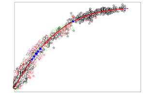
  $({C_m}/\alpha ){(D/d)^{1 - n}}{({f_e}/{f_{e,opt}})^m}$ exhibits a large scatter as Re varies from 5800 to 40 000 (figure 14). However, as shown in figure 15, it is, surprisingly, found that all the data of Ke/K 0, from more than 7000 AI-generated control laws or from conventional control (Perumal & Zhou Reference Perumal and Zhou2018), collapse well together, with a small scatter, once a weighting factor 1/Re is introduced in the abscissa, i.e.
 \begin{equation}\zeta = \frac{{{C_m}}}{\alpha }\; {\left( {\frac{D}{d}} \right)^{1 - n}}\frac{1}{{Re}}{\left( {\frac{{{f_e}}}{{{f_{e,opt}}}}} \right)^m}.\end{equation}
Here, Ke = g 1 (Cm, fe/f 0, α, d/D, Re, K 0) is now reduced to Ke/K 0 = g 2  $(\zeta )$. The data may be least-square fitted to a cubic function, viz.
 \begin{equation}{K_e}/{K_0} = 2.2 \times {10^{12}}{\zeta ^3}-1.3 \times {10^9}{\zeta ^2} + 2.6 \times {10^5}\zeta + 1.0.\end{equation}
The measured Ke/K 0 may deviate from (5.6) by no more than 10 %, with a 95 % confidence. Apparently, Ke/K 0 is the jet entrainment ratio, indicating the enhancement of entrainment with respect to the unforced jet.

Figure 13. Dependence of Ke/K 0 on (a)  $({C_m}/\alpha ){(D/d)^{1 - n}}$ for different fe/fe,opt and (b)
  $({C_m}/\alpha ){(D/d)^{1 - n}}{({f_e}/{f_{e,opt}})^m}$ (α = 0.1–0.9; Re = 13 000).

Figure 14. Dependence of Ke/K 0 on  $({C_m}/\alpha ){(D/d)^{1 - n}}{({f_e}/{f_{e,opt}})^m}$ for Re = 5800–40 000 (α = 0.07–0.90, fe/f 0 = 0.1–1.5).

Figure 15. Dependence of Ke/K 0 on  $({C_m}/\alpha ){(D/d)^{1 - n}}(1/Re){({f_e}/{f_{e,opt}})^m}$ for Re = 5800–40 000, α = 0.07–0.9, fe/f 0 = 0.1–1.5. The red curve is the least-squares fit to experimental data. Blue filled symbols correspond to Ke,max/K 0, predicted from (5.6), at a given Re.
One may wonder whether the same scaling law (5.6) could be obtained from a small amount of data, say generated by 200 control laws instead of 7000. One test is then performed. To ensure various control performances are covered, all the control laws for a given Re are re-numbered based on their J values, and 25 control laws are selected with the same difference in J. The dependence of Ke/K 0 on  $({C_m}/\alpha ){(D/d)^{1 - n}}(1/Re){({f_e}/{f_{e,opt}})^m}$ (figure not shown) can be least-squares fitted to a curve almost identical to that shown in figure 15, albeit with very few data falling between ζ = (1.0–1.9) × 10−4, where Re is 5800. One may conclude that the confidence level of the scaling law would not drop appreciably in spite of a drop in the control laws from the order of 1000 to 25 for each Re, given Re ≥ 8000.
The way m is determined may imply a limited range of fe/fe,opt over which (5.6) is valid. As illustrated in figure 16, Ke/K 0 calculated from (5.6) agrees with measurement for Re = 8000 at (Cm, α, d/D) = (1.0 %, 0.5, 1/20) and (2.0 %, 0.3, 1/20), thus providing a validity for the choice of m. Note an appreciable deviation for fe/fe,opt ≥ 1.8 in Ke/K 0 between calculation and measurement at α = 0.5. The measured Ke/K 0 appears to change little for fe/fe,opt ≥ 1.8. Perumal & Zhou (Reference Perumal and Zhou2018) demonstrated that an unsteady minijet at large α (≥0.5) and fe/f 0 (≥1.0) behaves like a quasi-steady blowing, and jet mixing is independent of both α and fe/f 0, which accounts for the deviation. The observation suggests a critical fe/fe,opt beyond which the scaling law (5.6) is invalid, and this critical fe/fe,opt is the fe,steady/fe,opt value at which Ke/K 0 becomes independent of fe/fe,opt for a given α. Figure 17 presents the dependence on α of fe,steady/f 0, which is extracted from the data illustrated in figure 12(a) and least-square fitted to
 \begin{equation}{f_{e,steady}}/{f_0} ={-} 1.55{\alpha ^{1.1}} + 1.4.\end{equation}
Then, the critical fe/fe,opt or fe,steady/fe,opt at which (5.6) may deviate appreciably from the measured data can be obtained from (5.4) and (5.7), viz.
 \begin{equation}\frac{{{f_{e,steady}}}}{{{f_{e,opt}}}} = \; \frac{{{f_{e,steady}}/{f_0}}}{{{f_{e,opt}}/{f_0}}}.\end{equation}
Substitution of α = 0.5 into (5.4) and (5.7) yields fe,steady/fe,opt = 1.8, which is internally consistent with the observation from figure 16.

Figure 16. Comparison of the dependence of Ke/K 0 on fe/fe,opt for Re = 8000 between prediction from (5.6) (open symbol) and measurement (filled symbol) for (Cm, α, d/D) = (2.0 %, 0.3, 1/20) and (1.0 %, 0.5, 1/20). The rectangle highlights the deviation between prediction and measurement.
There is a need to understand the physical meaning of n, which may offer valuable insight into the flow physics behind control. The physical interpretation of n is given by Perumal & Zhou (Reference Perumal and Zhou2018) for a fixed Re. As d/D is decreased, say by half, one might have expected, given α = 0.1 and fe/f 0 = 0.5, that the required Cm would also reduce by 50 % to achieve the same Ke/K 0 (Re = 8000); yet, Cm was measured to drop by  $60\,\textrm{\%}$ (their figure 23). The additional 10 % drop results from the retardation effect of minijet injection with contracting d/D. That is, a non-zero n reflects the need for additional Cm to achieve the same Ke/K 0 for given α. Apparently, the retardation effect depends on α and Re (5.3). Perumal & Zhou (Reference Perumal and Zhou2018) have documented in detail the dependence of the retardation effect on α. Thus, we present only its dependence on Re. In order to determine the dependence of required Cm on Re to achieve the same Ke/K 0 at given fe/fe,opt, α and d/D, we rewrite (5.6) as
 \begin{equation}{K_e}/{K_0}\; \approx \; \; \frac{{{C_m}}}{\alpha }\; {\left( {\frac{D}{d}} \right)^{1 - n}}\frac{1}{{Re}}{\left( {\frac{{{f_e}}}{{{f_{e,opt}}}}} \right)^m}.\end{equation}
Rearranging (5.9) yields
 \begin{equation}{C_m} \approx Re{K_e}/{K_0}\alpha {\left( {\frac{d}{D}} \right)^{1 - n}}{\left( {\frac{{{f_{e,opt}}}}{{{f_e}}}} \right)^m}.\end{equation}
Equation (5.10) can be used to predict the required Cm with varying Re for a pre-specified Ke/K 0 at given fe/fe,opt,  $\alpha $ and d/D. It is of interest to compare the variation in Cm with Re for a given Ke/K 0 at the same fe/fe,opt,
  $\alpha $ and d/D with and without the retardation effect. On substitution of n = 0 in (5.10), we may obtain Cm in the absence of the retardation effect
 \begin{equation}{C_m} \approx Re{K_e}/{K_0}\alpha \left( {\frac{d}{D}} \right){\left( {\frac{{{f_{e,opt}}}}{{{f_e}}}} \right)^m}.\end{equation}
Figure 18 compares the dependence of Cm on Re (= 5800–40 000) for a pre-specified Ke/K 0 = 6 ( fe/fe,opt = 1.0, α = 0.1, d/D = 1/20) calculated from (5.11) with that from (5.10) where n is determined from (5.3a–c). Clearly, given the same Re, Cm calculated from (5.10) is substantially larger, as a result of the retardation effect, than that from (5.11). For example, at Re = 20 000, the Cm values from (5.10) and (5.11) are approximately 0.85 % and 0.22 %, respectively. The retardation effect may depend on Re, which is defined by the percentage increase in required Cm calculated from (5.10) as compared with (5.11), viz.
 \begin{equation}\Delta {C_m} = \; ({[{C_m}]_{(5.10)}} - \; {[{C_m}]_{(5.11)}})/{[{C_m}]_{(5.11)}}.\end{equation}
The value of  $\Delta {C_m}$ increases with Re for Re < 10 600 and becomes independent of Re for Re ≥ 10 600 (figure 18), as n does (figure 11b). At Re = 20 000, the required Cm to achieve a pre-specified Ke/K 0 = 6 ( fe/fe,opt = 1.0, α = 0.1, d/D = 1/20) from (5.10) is 2.8 times higher than from (5.11). Evidently, n plays a significant role in characterizing the retardation effect of the minijet, which contracts with increasing α and reaches zero at α = 0.9, where n ≈ 0 (Perumal & Zhou Reference Perumal and Zhou2018).

Figure 17. Dependence of fe,steady/f 0 on α extracted from the dependence of Ke/K 0 on fe/f 0, as illustrated in figure 12(a).


5.3. Physical interpretation of similarity parameters
Some interesting inferences can be made from the scaling law (figure 15 or (5.6)). Firstly, it is important to understand physically ξ/Re, where  $\xi = ({C_m}/\alpha ){(D/d)^{1 - n}}$ is interpreted as the effective penetration depth at a given Re = 8000 (Perumal & Zhou Reference Perumal and Zhou2018). Yang et al. (Reference Yang, Zhou, So and Liu2016) and Perumal & Zhou (Reference Perumal and Zhou2018) demonstrated that the distribution of
  $u_{rms}^\ast $ at the nozzle exit and the minijet penetration depth into the main jet are correlated. Figure 19 shows the radial distributions of
  $u_{rms}^\ast{=} \; {u_{rms}}/{\bar{U}_j}$ measured at x* = 0.05 ( fe/fe,opt = 1) along the injection (x–y) plane for ξ/Re = 0.3 × 10⁻⁴ at Re = 8000, 13 000 and 20 000. Interestingly, given the same ξ/Re, the
  $u_{rms}^\ast $ distributions are qualitatively the same despite different combinations of Cm, α, d/D and Re, suggesting that the penetration depth, as marked in figure 19, is the same given the same ξ/Re, that is, there is a correspondence between ξ/Re and the penetration depth. Perumal & Zhou (Reference Perumal and Zhou2018) pointed out that ξ is physically the effective momentum ratio of the minijet to the main jet per pulse of injection or the effective penetration depth for a fixed Re. The present finding points to the fact that
  $\xi /Re$ is a more general definition for the effective momentum ratio of the minijet to the main jet per pulse of injection, which is valid even in the context of varying Re.

Figure 19. Radial distributions of the streamwise fluctuating velocity  $u_{rms}^\ast{=} \; {u_{rms}}/{\bar{U}_j}$ measured at x* = 0.05 ( fe/fe,opt = 1) for
  $\xi $/Re = 0.3*10−4.
Secondly, to gain insight into the physics behind fe/fe,opt, we present in figure 20(a1–c2) typical images from flow visualization (Re = 8000) in the injection plane (x–z) for fe/fe,opt < 1, fe/fe,opt = 1 and fe/fe,opt > 1 at ξ/Re = 0.3 × 10⁻⁴, along with the signals of instantaneous streamwise U* measured at (x ∗, y*, z*) = (1.5, 0, 0.45). The sharp peaks in the signals represent the perturbation induced by the injection. Once manipulated, the shear layer rolls up early on the injection side (cf. unforced flow shown in figure 3b) and the vortex dynamics is very different, depending on fe/fe,opt. There exist three different states of the manipulated jet depending on fe/fe,opt. State 1 corresponds to fe/fe,opt = 1, at which the optimal separation takes place between incomplete ring vortices. As shown in figure 20(b1), an incomplete ring vortex V 2 induced by minijet injection is advected downstream without direct interaction with a following vortex V 1 induced by the next cycle of injection. This assertion is complemented by the velocity signal in figure 20(a1), where the peaks are distinctly separated. It seems plausible that the ring vortices with the minimum but clear separation produce the maximized jet decay rate (figure 16). State 2 corresponds to a smaller fe/fe,opt (= 0.57) or an increased gap between the successive ring vortices, as shown in figure 20(a2,b2). Evidently, the incomplete ring vortex V 4 needs more time to grow before interacting with the next one V 3. This increased gap seems to facilitate the establishment of less anti-symmetrically arranged vortices about the centreline in the (x–y) plane (figure 20a2, cf. figure 20a1), resembling more a natural jet and resulting in a reduced jet decay rate (figure 16). Under state 3, where fe/fe,opt > 1, the spatial separation between the vortices V 5 and V 6 contracts, as illustrated in figure 20c2 ( fe/fe,opt = 1.71), and the interaction between the vortices is intensified. This is corroborated by the hot-wire signal (figure 20c1), which shows the peaks closely separated from each other. This interaction may incur the occurrence of turbulent puff-like structures, causing a retreat of penetration (Hermanson, Wahba & Johari Reference Hermanson, Wahba and Johari1998; Johari Reference Johari2006) and weakened mixing. Johari, Pacheco-Tougas & Hermanson (Reference Johari, Pacheco-Tougas and Hermanson1999) made a similar observation for jet in cross-flow and pointed out that a decrease in spacing between the vortical structures resulted in increased interaction and reduced penetration. Thus, the jet decay rate under state 3 also drops compared with state 1 (figure 16). The three states observed at Re = 8000 are also evident at other Re (not shown) given an identical ξ/Re. The similarity parameter fe/fe,opt on which states 1–3 strongly depend physically corresponds to the spatial separation between successive vortices formed during minijet injection (figure 20a2–c2). Thus, the jet mixing depends on the penetration depth of the minijet into the main jet (ξ/Re) and the interaction between vortices ( fe/fe,opt) in the manipulated jet, and ζ is physically the momentum ratio (the momentum per pulse of injection to the inertia momentum of main jet) times the frequency ratio.

Figure 20. (a1–c1) Typical U* signals measured at (x ∗, y*, z*) = (1.5, 0, 0.45) for fe/fe,opt = 0.57, 1 and 1.71 at  $\xi $/Re = 0.3 × 10⁻⁴ for Re = 8000. (a2–c2) Typical flow structures from flow visualization in the injection plane (x–z) at representative fe/fe,opt, where the vortices V 1–V 6 result from minijet injection at
  $\xi $/Re = 0.3 × 10⁻⁴ for Re = 8000.
Thirdly, the ratio Ke,max/K 0 drops rapidly with increasing Re for Re < 10 600 but very slowly for Re ≥ 10 600 (figure 21), which may be described by
 \begin{equation}{K_{e,max}}/{K_0} \approx 2.24\ast {10^{15}}R{e^{ - 3.7}} + 6.8.\end{equation}
This feature is primarily due to the variation in K 0 with increasing Re (figure 9) as Ke,max is unchanged (figure 7). As such,  $\zeta = (\xi /Re){({f_e}/{f_{e,opt}})^m}$ and
  ${\xi _{opt}} = {((\sqrt {MR} /\alpha ){(d/D)^n})_{opt}}$ at which Ke,max/K 0 occurs. Then, at fe/fe,opt = 1, (5.9) may be rewritten as
 \begin{equation}{K_{e,max}}/{K_0}\; \approx \; {\left( {\frac{{\sqrt {MR} }}{\alpha }\; {{\left( {\frac{d}{D}} \right)}^n}} \right)_{opt}}\frac{1}{{Re}}{\left( {\frac{{{f_{e,opt}}}}{{{f_{e,opt}}}}} \right)^{0.7}} = \frac{{{\xi _{opt}}}}{{Re}} = {\zeta _{opt}}.\end{equation}
Thus, given Re, Ke,max/K 0 may be estimated from (5.13). As  ${\zeta _{opt}} = {\xi _{opt}}/Re$ is connected to the effective penetration depth of the minijet into main jet and hence Ke/K 0, the drop in Ke,max/K 0 with Re can be directly correlated to the reduced effective minijet penetration into main jet measured in terms of
  ${\xi _{opt}}/Re$. One may wonder why the effective penetration depth or
  ${\xi _{opt}}/Re$ contracts with increasing Re. Figure 21 presents a variation with Re in the normalized stroke length L/d determined at Ke,max/K 0. Physically, L represents the slug of jet fluid ejected during each pulse of injection or the amount of fluid injected during one injection (Steinfurth & Weiss Reference Steinfurth and Weiss2020) and, following Johari (Reference Johari2006), is estimated by
  $L = (1/{A_m})\int_0^{{\tau _{opt}}} {\int_A {{U_{m\; }}\,\textrm{d}{A_m}\,\textrm{d}t} } = {\bar{U}_m}{\tau _{opt}}$, where
  ${\tau _{opt}} = \alpha /{f_{e,opt}}$, the minijet velocity
  ${\bar{U}_m} = \; {C_m}\; {(D/d)^2}{\bar{U}_j}$ (Perumal & Zhou Reference Perumal and Zhou2018) and Am is the minijet exit area. Johari (Reference Johari2006) found that the minijet-generated flow structure depended on L/d, characterized by turbulent puffs for 25 < L/d < 75 and an elongated steady jet structure for L/d > 75, and the penetration depth of the latter was significantly smaller than that of the former. Figure 21 shows that L/d grows with Re and indeed exceeds 75 for Re ≥ 10 600. This provides an explanation for the observation that Ke,max/K 0 or
  ${\xi _{opt}}/Re$ drops greatly from Re = 8000 to 10 600 (figure 21).


Fourthly, given a pre-specified Ke/K 0 = 6 and ( $\alpha $, d/D) = (0.1, 1/20), we may determine the relation between Cm and Re from (5.10) for fe/fe,opt = 0.57, 1.0 and 1.71. Figure 22 shows that Cm is always least at fe/fe,opt = 1.0, regardless of Re.

Figure 22. Dependence of Cm on Re for fe/fe,opt = 1.0, <1.0 and >1.0 (α = 0.1, d/D = 1/20), predicted from (5.10) for a pre-defined Ke/K 0 = 6.
Finally, Wickersham (Reference Wickersham2007) investigated the effect of excitation frequency of pulsed injection on a jet of Re = 71 000–355 000 manipulated by two pulsed injections. They argued that, under the optimal pulsing condition, the minijet penetrated farther into the jet and the induced vortices were able to persist longer downstream, thus enhancing mixing. In the study of a pulsed jet in cross-flow, Johari (Reference Johari2006) also reported that the maximum mixing can be achieved with pulsed jets if the pulsing parameters are chosen specifically to create compact vortex rings and subsequent interaction among vortical structures. Nevertheless, to the best of our knowledge, there has been no report in the literature on the parameters that determine the optimal pulsing condition. This condition is evident from (5.14), determined by ξopt /Re and fe/fe,opt = 1, and hence  ${\zeta _{opt}}$, that is, Ke,max/K 0 is achieved at the maximum penetration ξopt /Re and meanwhile the vortices thus formed under minijet injection are optimally separated from each other, as dictated by fe/fe,opt = 1.
6. Conclusions
A novel hybrid AI system has been developed to manipulate a turbulent jet using a single pulsed radial minijet over a range of Re (= 5800–40 000). Four control parameters are investigated, i.e. Cm (= 0.1 %–8.0 %), fe/f 0 (= 0–1.2), α (= 0.1–0.9) and d/D (= 1/20, 1/40). The following conclusions can be drawn out of this work:
(i) The developed hybrid AI algorithm may optimize simultaneously a control law and a time-independent variable Cm, overcoming the drawback of the previous AI system based on the LGP algorithm that can be used to optimize only the control laws (e.g. Zhou et al. Reference Zhou, Fan, Zhang, Li and Noack2020). At Re = 8000, for example, the system successfully finds the optimal control law, which consists of two sub-control laws that govern a time-dependent pulse signal b1(t) (α = 7 %, fe/f 0 = 0.52) and a time-independent mass flow rate signal b 2 (Cm = 1.2 %), respectively. Proximity map analysis performed based on all the control laws reveals that the ratio Cm/α, corresponding physically to the penetration depth of the pulsed minijet, dictates the control performance (figure 8). The system exhibits good robustness as Re varies from 5800 to 40 000, finding essentially the same maximum Ke and the same optimal fe/f 0.
(ii) The AI system produces more than 7000 control laws for eight Re values examined and subsequently a tremendous amount of data involving six intrinsically related variables Ke, K 0, Cm, fe/f 0, α and Re. Careful analysis of the data, along with those produced from a conventional open-loop control technique, which include one more variable, d/D, unveils, surprisingly, a scaling law, that is, the relationship Ke = g 1 (Cm, fe/f 0, α, d/D, Re, K 0) may be reduced to Ke/K 0 = g 2
 $(\zeta )$, where the scaling factor $\zeta = ({C_m}/\alpha ){(D/d)^{1 - n}}(1/Re){({f_e}/{f_{e,opt}})^m}$. This law governs the effect of Re on jet manipulation using an unsteady minijet. Here, Ke/K 0 accounts for the effect of Re on the control performance, while ζ is physically the momentum ratio $({C_m}/\alpha ){(D/d)^{1 - n}}(1/Re)$ (the momentum per pulse of minijet injection to the inertia momentum of the main jet) times the frequency ratio ${({f_e}/{f_{e,opt}})^m}$, the latter providing a measure for the spatial separation between successive vortices (figure 20a2–c2). The manipulated jet may exhibit three states, i.e. state 1 – fe/fe,opt = 1, state 2 – fe/fe,opt > 1 and state 3 – fe/fe,opt < 1, dictated by ${({f_e}/{f_{e,opt}})^m}$. State 1 is associated with the optimally separated vortices, resulting in Ke,max/K 0, while states 2 and 3 yield closely and over-separated vortices, respectively, both causing a decline in Ke/K 0 (figure 16).
(iii) Several inferences can be made from the scaling law. Firstly, Ke/K 0 increases with ζ. Secondly, given that
$\xi = ({C_m}/\alpha ){(D/d)^{1 - n}}$ may be interpreted as the effective momentum ratio of the minijet per pulse of injection to the main jet at a given Re (Perumal & Zhou Reference Perumal and Zhou2018), ξ /Re carries the same physical meaning, although with a more general sense, valid even in the context of varying Re. Thirdly, with $\zeta = (\xi /Re){({f_e}/{f_{e,opt}})^m},{\zeta _{opt}}$ at which Ke,max/K 0 occurs for any given Re depends on ξopt and $({f_e}/{f_0})_{opt}^m$. The value of ξopt drops from Re = 8000 to 10 600 and then rises for a further increase in Re (figure 21). Evidently, jet mixing depends on both the penetration depth and the interaction between vortices or ξ /Re and ${({f_e}/{f_{e,opt}})^m}$, whose optimum values lead to the maximized mixing. The optimal pulsing condition at which the maximum effective penetration of the minijet into the main jet occurs corresponds to ξopt (Wickersham Reference Wickersham2007). At fe/fe,opt = 1, the minijet creates compact vortex rings (Johari Reference Johari2006), which may persist farther downstream (Wickersham Reference Wickersham2007), thus maximizing jet mixing. The similarity parameter $\zeta $ unveils that, for given $\alpha $, the required Cm to achieve a pre-defined jet mixing or a constant Ke/K 0 is the smallest at fe/fe,opt = 1 or the most efficient, irrespective of Re (figure 22). Finally, with increasing Re, Ke ,max/K 0 diminishes rapidly for Re < 10 600 but very slowly for Re ≥ 10 600 (figure 21). The stroke length ratio L/d rises with Re (figure 21). Once L/d exceeds 75, the minijet flow structure is characterized by turbulent puffs, associated with the distributed vorticity and greater entrainment rate (Johari Reference Johari2006), instead of vortex rings, resulting in a reduced effective penetration depth and hence a smaller Ke ,max/K 0.


Funding
Y.Z. wishes to acknowledge support given to him from NSFC through grant 91752109 and from the Research Grants Council of the Shenzhen Government through grants JCYJ20190806143611025 and JCYJ20210324132816040. A.K.P. is grateful for Science and Engineering Research Board, Department of Science and Technology, through Grant No. EEQ/2018/000179.
Declaration of interests
The authors report no conflict of interest.


