


1. Introduction
Bubble–particle collisions are central to the flotation process, which is widely used (e.g. in the mining industry) to separate minerals through their attachment to rising bubbles. This intricate process involves a wide range of colloid science disciplines (Derjaguin & Dukhin Reference Derjaguin and Dukhin1993; Nguyen & Schulze Reference Nguyen and Schulze2003; Kostoglou, Karapantsios & Oikonomidou Reference Kostoglou, Karapantsios and Oikonomidou2020b ), with significant complexity stemming from the interplay of hydrodynamics and physicochemical interactions. The hydrodynamic bubble–particle interaction remains of paramount importance for optimisation, as it is the rate-determining step that also sets the conditions for other interactions.
Most of the work on bubble–particle collisions draws on the large body of work on particle–particle collisions (Pumir & Wilkinson Reference Pumir and Wilkinson2016), in particular the seminal work of Saffman & Turner (Reference Saffman and Turner1956) for the tracer limit and the model proposed by Abrahamson (Reference Abrahamson1975) for the kinetic gas limit at large particle inertia. Such models predict the collision rate without considering the hydrodynamic interaction between the collision partners, but must take into account effects such as the segregation of bubbles and particles in a turbulent flow (Chan, Ng & Krug Reference Chan, Ng and Krug2023). However, the significant size difference between the larger bubble and the mineral particles in a typical flotation process makes it important to account for the flow distortion around the bubble. This can cause an encountering particle to be deflected, reducing the actual number of collisions. For a bubble rising in quiescent flow, this process is deterministic and has been studied widely (Schulze Reference Schulze1989; Nguyen & Schulze Reference Nguyen and Schulze2003; Sarrot, Guiraud & Legendre Reference Sarrot, Guiraud and Legendre2005; Huang, Legendre & Guiraud Reference Huang, Legendre and Guiraud2012). In this case, the effect of the hydrodynamic interaction can be captured in terms of a collision efficiency, which relates the rate of actual collisions to the encounter rate. The lack of a suitable concept to account for turbulence in this context is widely acknowledged in the literature (Pyke, Fornasiero & Ralston Reference Pyke, Fornasiero and Ralston2003; Nguyen et al. Reference Nguyen, An-Vo, Tran-Cong and Evans2016; Hajisharifi, Marchioli & Soldati Reference Hajisharifi, Marchioli and Soldati2021). Existing approaches are flawed because they combine turbulent encounter rates with collision efficiencies applicable to pure gravitational settling (Bloom & Heindel Reference Bloom and Heindel2002; Koh & Schwarz Reference Koh and Schwarz2007; Liu & Schwarz Reference Liu and Schwarz2009; Yoon et al. Reference Yoon, Soni, Huang, Park and Pan2016). Others use a Reynolds-type decomposition, which is problematic given the strongly nonlinear dependence of the problem on the flow velocity. Another conceptual inconsistency is that the encounter rate is based on the bubble–particle relative velocity, whereas the collision efficiency is determined by the bubble slip relative to the fluid. Some of these deficiencies are overcome by the collision model presented in Kostoglou, Karapantsios & Evgenidis (Reference Kostoglou, Karapantsios and Evgenidis2020a ), but this, however, remains limited to tracer particles.
The core problem is to determine the collision rate of small inertial particles with a finite-size object in a turbulent flow. This is of general relevance to many other applications beyond flotation, such as the collision of cloud droplets (Falkovich, Fouxon & Stepanov Reference Falkovich, Fouxon and Stepanov2002; Poydenot & Andreotti Reference Poydenot and Andreotti2024), the accretion of planetesimals by the collection of dust particles (Guillot, Ida & Ormel Reference Guillot, Ida and Ormel2014; Homann et al. Reference Homann, Guillot, Bec, Ormel, Ida and Tanga2016), depth filtration (May & Clifford Reference May and Clifford1967; Cushing & Lawler Reference Cushing and Lawler1998), or bacterial degradation of marine snow (Arguedas-Leiva et al. Reference Arguedas-Leiva, Słomka, Lalescu, Stocker and Wilczek2022). However, the scarcity of data, due to the difficulties in performing the necessary experiments and interface-resolved simulations, has hindered the progress of theoretical research in this area. In this paper, we present a combined numerical and theoretical study of the effects of turbulence on bubble–particle collisions using direct numerical simulations. We adopt homogeneous and isotropic turbulence (HIT), in which we measure how turbulent fluctuation modifies the bubble–particle collision rate along the bubble-rising path.
2. Statistical model
The collision frequency
 $K$
of particles with a bubble is determined by
$K$
of particles with a bubble is determined by
 $K = \Gamma n_p$
, where
$K = \Gamma n_p$
, where
 $n_p$
is the particle number density, and the proportionality coefficient
$n_p$
is the particle number density, and the proportionality coefficient
 $\Gamma$
(
$\Gamma$
(
 $\rm m^3\,s^{-1}$
) is commonly referred to as the collision kernel and is determined by the flow (Pumir & Wilkinson Reference Pumir and Wilkinson2016). In quiescent flow, the collisions between a spherical bubble of radius
$\rm m^3\,s^{-1}$
) is commonly referred to as the collision kernel and is determined by the flow (Pumir & Wilkinson Reference Pumir and Wilkinson2016). In quiescent flow, the collisions between a spherical bubble of radius
 $r_b$
rising at constant velocity
$r_b$
rising at constant velocity
 $U_b$
with small inertial solid particles are deterministic. The particle grazing trajectory
$U_b$
with small inertial solid particles are deterministic. The particle grazing trajectory
 $\Psi _c$
determines a ‘collision tube’, where all the particles contained inside collide with the bubble, as illustrated in figure 1(a). In this case, the collision frequency is determined by the collision number flux, i.e.
$\Psi _c$
determines a ‘collision tube’, where all the particles contained inside collide with the bubble, as illustrated in figure 1(a). In this case, the collision frequency is determined by the collision number flux, i.e.
 $K=Q_cn_p$
. The collision number flux
$K=Q_cn_p$
. The collision number flux
 $Q_c$
can be determined by the cross-sectional area of radius
$Q_c$
can be determined by the cross-sectional area of radius
 $r_c$
limited by the grazing trajectories upstream far from the bubble:
$r_c$
limited by the grazing trajectories upstream far from the bubble:
 $Q_c=\pi r_c^2U_b$
. Therefore, the collision kernel in quiescent flow can be expressed as
$Q_c=\pi r_c^2U_b$
. Therefore, the collision kernel in quiescent flow can be expressed as
 $\Gamma _q=Q_c=\pi r_b^2U_bE_c$
, where the collision efficiency
$\Gamma _q=Q_c=\pi r_b^2U_bE_c$
, where the collision efficiency
 $E_c=r_c^2/r_b^2$
measures the ratio of collided particle number to the total encountering particle number. Notice here that
$E_c=r_c^2/r_b^2$
measures the ratio of collided particle number to the total encountering particle number. Notice here that
 $E_c$
depends on the bubble Reynolds number
$E_c$
depends on the bubble Reynolds number
 $Re_b=2r_bU_b/\nu$
, the ratio of the particle radius
$Re_b=2r_bU_b/\nu$
, the ratio of the particle radius
 $r_p$
and
$r_p$
and
 $r_b$
, and the Stokes number
$r_b$
, and the Stokes number
 $St_p = \tau _p/\tau _f$
, with
$St_p = \tau _p/\tau _f$
, with
 $\tau _p$
the particle response time, and
$\tau _p$
the particle response time, and
 $\tau _f = 2r_b/U_b$
the time scale of the bubble–particle interaction (Dai, Fornasiero & Ralston Reference Dai, Fornasiero and Ralston2000; Sarrot et al. Reference Sarrot, Guiraud and Legendre2005; Huang et al. Reference Huang, Legendre and Guiraud2012).
$\tau _f = 2r_b/U_b$
the time scale of the bubble–particle interaction (Dai, Fornasiero & Ralston Reference Dai, Fornasiero and Ralston2000; Sarrot et al. Reference Sarrot, Guiraud and Legendre2005; Huang et al. Reference Huang, Legendre and Guiraud2012).
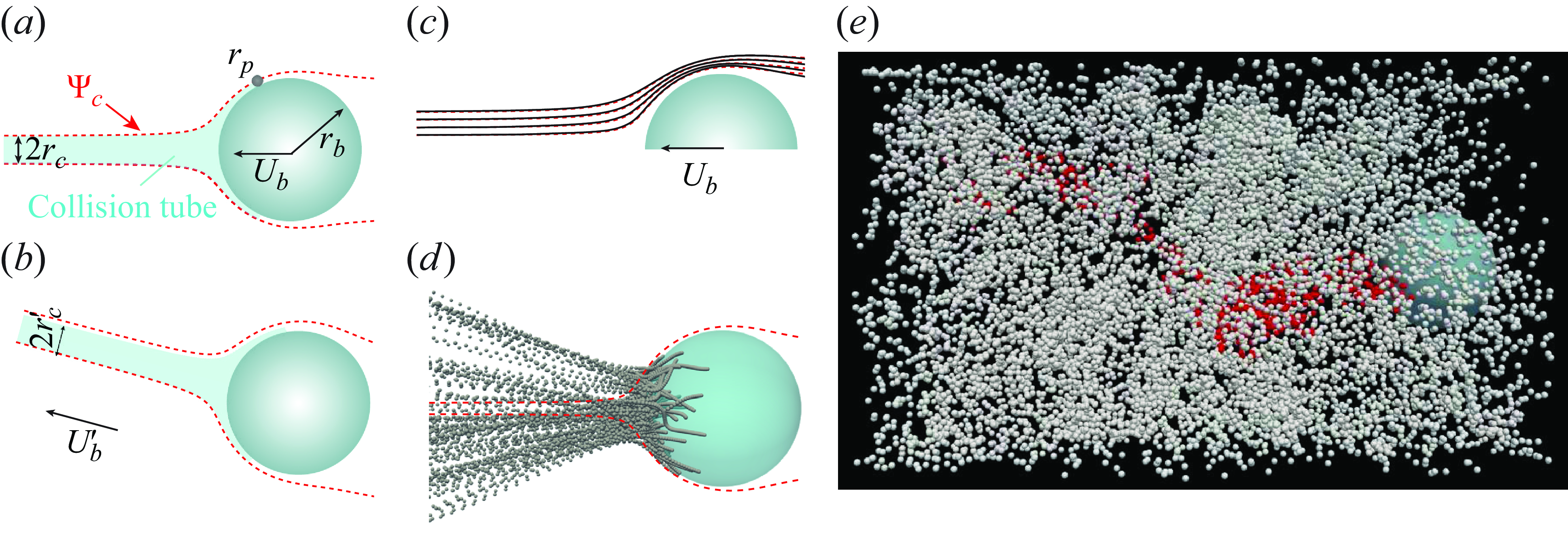
Figure 1. (a) Sketch of the grazing trajectory (red dashed line) in quiescent flow. The shaded region indicates the collision tube where all particles collide on the bubble. (b) Sketch of the bubble–particle collision model under temporary bubble slip velocity
 $U'_{b}$
. (c) Mean flow streamlines around the bubble for the case of imposed velocity bubble (solid) and quiescent flow (dashed lines) at
$U'_{b}$
. (c) Mean flow streamlines around the bubble for the case of imposed velocity bubble (solid) and quiescent flow (dashed lines) at
 $\overline {Re_b}=120$
. (d) Trajectories of colliding particles (
$\overline {Re_b}=120$
. (d) Trajectories of colliding particles (
 $r_p/r_b=0.05,\ St_p=0.04$
) for the case of imposed velocity bubble compared to the corresponding grazing trajectories (red lines) in quiescent flow at the same
$r_p/r_b=0.05,\ St_p=0.04$
) for the case of imposed velocity bubble compared to the corresponding grazing trajectories (red lines) in quiescent flow at the same
 $Re_b =120$
. (e) Snapshot of the bubble–particle collision process in turbulence for the imposed-velocity bubble with flow from left to right in the bubble frame of reference. Incoming particles that end up colliding with the bubble are marked in red.
$Re_b =120$
. (e) Snapshot of the bubble–particle collision process in turbulence for the imposed-velocity bubble with flow from left to right in the bubble frame of reference. Incoming particles that end up colliding with the bubble are marked in red.
To provide an understanding of the relevant physical mechanisms of bubble–particle collision in turbulence, we propose a statistical model. We start from the assumption that the flow field in the vicinity of the bubble is approximately stationary and uniform during the bubble–particle interaction. Conceptually, this implies that the temporal scale
 $\tau _f$
is (much) shorter than the correlation time scale of flow fluctuations (
$\tau _f$
is (much) shorter than the correlation time scale of flow fluctuations (
 $O(\tau _\eta )$
), but it remains to be tested from the data under what conditions exactly this assumption is valid in practice. Additionally, we consider the flow correlation length scale to be comparable to or larger than the bubble size. Within this ‘frozen turbulence’ assumption, the instantaneous bubble–particle collision process in turbulence can be related back to that observed in quiescent flow. Therefore, the equivalent steady flow problem is characterised by the magnitude of the instantaneous bubble slip velocity
$O(\tau _\eta )$
), but it remains to be tested from the data under what conditions exactly this assumption is valid in practice. Additionally, we consider the flow correlation length scale to be comparable to or larger than the bubble size. Within this ‘frozen turbulence’ assumption, the instantaneous bubble–particle collision process in turbulence can be related back to that observed in quiescent flow. Therefore, the equivalent steady flow problem is characterised by the magnitude of the instantaneous bubble slip velocity
 $U'_{b}$
with corresponding values
$U'_{b}$
with corresponding values
 $Re'_{b} = 2r_bU'_{b}/\nu$
and
$Re'_{b} = 2r_bU'_{b}/\nu$
and
 $St'_{p}=\tau _p/(2r_b/U'_{b})$
, as shown in figure 1(b). The entire bubble–particle collision process in a turbulent flow can then be viewed as a superposition of collision events in quiescent flow with varying parameters
$St'_{p}=\tau _p/(2r_b/U'_{b})$
, as shown in figure 1(b). The entire bubble–particle collision process in a turbulent flow can then be viewed as a superposition of collision events in quiescent flow with varying parameters
 $Re'_{b}$
and
$Re'_{b}$
and
 $St'_{p}$
. In the framework, the collision number
$St'_{p}$
. In the framework, the collision number
 $N_c|_{\Delta \tau }$
during a short period
$N_c|_{\Delta \tau }$
during a short period
 $\Delta \tau$
(
$\Delta \tau$
(
 $O(\tau _\eta )$
) in turbulent flow, with mean particle number density
$O(\tau _\eta )$
) in turbulent flow, with mean particle number density
 $n_p$
, is given by
$n_p$
, is given by
 $N_c|_{\Delta \tau }=\pi r_b^2E_c(Re'_{b},St'_{p})U'_{b}n'_p\,\Delta \tau$
, where
$N_c|_{\Delta \tau }=\pi r_b^2E_c(Re'_{b},St'_{p})U'_{b}n'_p\,\Delta \tau$
, where
 $n'_{p}$
is the instantaneous encountering particle number density, which depends on
$n'_{p}$
is the instantaneous encountering particle number density, which depends on
 $Re'_{b}$
and
$Re'_{b}$
and
 $St'_{p}$
. Importantly,
$St'_{p}$
. Importantly,
 $E_c(Re'_{b},\ St'_{p})$
denotes the collision efficiency in quiescent flow for varying flow parameters, which is deterministic and can be parametrised. Then the total expected collision number
$E_c(Re'_{b},\ St'_{p})$
denotes the collision efficiency in quiescent flow for varying flow parameters, which is deterministic and can be parametrised. Then the total expected collision number
 $N_c$
during a sufficiently long time period
$N_c$
during a sufficiently long time period
 $T=\sum \Delta \tau$
is given by
$T=\sum \Delta \tau$
is given by
 \begin{equation} N_c = \pi r_b^2T\int E_c(Re'_{b},\ St'_{p})\,U'_{b}f(U'_{b})n'_{p}\,{\rm d}U'_{b}. \end{equation}
Based on this, the collision kernel can be derived as
 \begin{equation} \Gamma = \frac {K}{n_p}={\frac {\pi r_b^2}{n_p}\int E_c(Re'_{b},\ St'_{p})\,U'_{b}\,f(U'_{b})\,n'_{p}\,\textrm {d} U'_{b}}. \end{equation}
Note that collision efficiency has been studied extensively, and the general dependence of
 $E_c$
on the bubble Reynolds number and particle Stokes number has been established in the literature (Schulze Reference Schulze1989; Sarrot, Guiraud & Legendre Reference Sarrot, Guiraud and Legendre2005; Huang et al. Reference Huang, Legendre and Guiraud2012). The collision kernel is thus determined by the probability density function (PDF)
$E_c$
on the bubble Reynolds number and particle Stokes number has been established in the literature (Schulze Reference Schulze1989; Sarrot, Guiraud & Legendre Reference Sarrot, Guiraud and Legendre2005; Huang et al. Reference Huang, Legendre and Guiraud2012). The collision kernel is thus determined by the probability density function (PDF)
 $f(U'_{b})$
of the bubble slip velocity
$f(U'_{b})$
of the bubble slip velocity
 $U'_{b}$
, the modelling of which remains an open question. Furthermore, we note that the collision kernel will also be affected by the preferential sampling for particles with large
$U'_{b}$
, the modelling of which remains an open question. Furthermore, we note that the collision kernel will also be affected by the preferential sampling for particles with large
 $St_p$
, as this alters the incoming particle number density.
$St_p$
, as this alters the incoming particle number density.
3. Numerical methods and simulations
We perform interface-resolved direct numerical simulations (DNS) to test this model. The turbulent flow is governed by the incompressible Navier–Stokes equations, which read
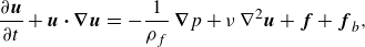 \begin{eqnarray} \frac {\partial \boldsymbol{u}}{\partial t} + \boldsymbol{u}\boldsymbol{\cdot} \boldsymbol{\nabla } \boldsymbol{u} &=& - \frac {1}{\rho _f}\,\boldsymbol{\nabla } p + \nu \, \nabla ^2 \boldsymbol{u} + \boldsymbol{f} + \boldsymbol{f}_b, \end{eqnarray}
 \begin{eqnarray} \boldsymbol{\nabla } \boldsymbol{\cdot} \boldsymbol{u} &=& 0, \end{eqnarray}
where
 $\boldsymbol{u}$
is the fluid velocity,
$\boldsymbol{u}$
is the fluid velocity,
 $p$
denotes the pressure, and the parameters are the kinematic viscosity
$p$
denotes the pressure, and the parameters are the kinematic viscosity
 $\nu$
and the reference liquid density
$\nu$
and the reference liquid density
 $\rho _f$
. The vector
$\rho _f$
. The vector
 $\boldsymbol{f}$
denotes an external random large-scale volume force, which is statistically homogeneous and isotropic, with constant-in-time global energy input (Perlekar et al. Reference Perlekar, Biferale, Sbragaglia, Srivastava and Toschi2012). This force is used to generate and maintain the turbulent flow. The bubble-free turbulent flow intensity is characterised by the Reynolds number based on the Taylor microscale,
$\boldsymbol{f}$
denotes an external random large-scale volume force, which is statistically homogeneous and isotropic, with constant-in-time global energy input (Perlekar et al. Reference Perlekar, Biferale, Sbragaglia, Srivastava and Toschi2012). This force is used to generate and maintain the turbulent flow. The bubble-free turbulent flow intensity is characterised by the Reynolds number based on the Taylor microscale,
 $Re_\lambda =\sqrt {15u'/(\nu \epsilon )}$
, where
$Re_\lambda =\sqrt {15u'/(\nu \epsilon )}$
, where
 $u'$
denotes the root mean square velocity of the turbulence, and
$u'$
denotes the root mean square velocity of the turbulence, and
 $\epsilon$
is the mean energy dissipation rate. The vector
$\epsilon$
is the mean energy dissipation rate. The vector
 $\boldsymbol{f}_b$
accounts for the bubble–fluid two-way coupling.
$\boldsymbol{f}_b$
accounts for the bubble–fluid two-way coupling.
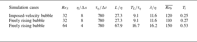
Table 1. Parameter of the numerical simulations and relevant turbulence scales:
 $Re_\lambda$
is the Taylor–Reynolds number;
$Re_\lambda$
is the Taylor–Reynolds number;
 $\eta =(\nu ^3/\epsilon )^{1/4}$
is the Kolmogorov dissipation length scale in grid space units
$\eta =(\nu ^3/\epsilon )^{1/4}$
is the Kolmogorov dissipation length scale in grid space units
 $\Delta x$
;
$\Delta x$
;
 $\tau _\eta$
is the Kolmogorov time scale in time-step units
$\tau _\eta$
is the Kolmogorov time scale in time-step units
 $\Delta t$
;
$\Delta t$
;
 $L=u'^3/\epsilon$
is the integral scale;
$L=u'^3/\epsilon$
is the integral scale;
 $T_L=L/u'$
is the large-eddy turnover time;
$T_L=L/u'$
is the large-eddy turnover time;
 $\lambda = u'\sqrt {15 \nu / \epsilon }$
is the Taylor micro-scale;
$\lambda = u'\sqrt {15 \nu / \epsilon }$
is the Taylor micro-scale;
 $\overline {Re_b}=2r_b\overline {U_b}/\nu$
is the bubble Reynolds number based on the mean rising velocity
$\overline {Re_b}=2r_b\overline {U_b}/\nu$
is the bubble Reynolds number based on the mean rising velocity
 $\overline {U_b}$
;
$\overline {U_b}$
;
 $T_i=u'/\overline {U_b}$
is the turbulent intensity.
$T_i=u'/\overline {U_b}$
is the turbulent intensity.
In the practice of flotation, commonly a large amount of surfactants is present in the liquid. Therefore, it is reasonable to assume that the bubbles with a typical Reynolds number below 200 are fully contaminated and approximately spherical, resulting in a boundary condition that is nearly no-slip (Nguyen & Schulze Reference Nguyen and Schulze2003; Huang et al. Reference Huang, Legendre and Guiraud2012). The Weber number
 $We=2r_b\rho _f U_b^2/\chi$
based on the surface tension
$We=2r_b\rho _f U_b^2/\chi$
based on the surface tension
 $\chi$
of water and the bubble rise velocity is
$\chi$
of water and the bubble rise velocity is
 $O(0.1)$
for our simulations, and even lower based on turbulent fluctuations. Therefore, bubble deformations remain negligible even if surface tension is lowered by the presence of surfactants. Under these conditions, the bubble behaves similarly to buoyant spheres. In this case, the translation and rotation of the bubble are governed by the Newton–Euler equations
$O(0.1)$
for our simulations, and even lower based on turbulent fluctuations. Therefore, bubble deformations remain negligible even if surface tension is lowered by the presence of surfactants. Under these conditions, the bubble behaves similarly to buoyant spheres. In this case, the translation and rotation of the bubble are governed by the Newton–Euler equations
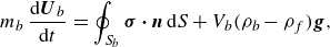 \begin{eqnarray} m_b\, \frac {{\rm d} \boldsymbol{U}_b}{\textrm {d}t} &=& \oint _{S_b} \boldsymbol {\sigma } \boldsymbol{\cdot} \boldsymbol{n}\, \textrm {d}S + V_b(\rho _b-\rho _f)\boldsymbol{g}, \end{eqnarray}
 \begin{eqnarray} \frac {\textrm {d} \boldsymbol {{I}} \boldsymbol{\Omega }}{\textrm {d}t} &=& \oint _{S_b} (\boldsymbol{x}-\boldsymbol{x}_b) \times (\boldsymbol {\sigma } \boldsymbol{\cdot} \boldsymbol{n})\, \textrm {d}S, \end{eqnarray}
where
 $\boldsymbol{U}_b(t)=\textrm {d}\boldsymbol{x}_b/\textrm {d}t$
and
$\boldsymbol{U}_b(t)=\textrm {d}\boldsymbol{x}_b/\textrm {d}t$
and
 $\mathbf {\Omega }(t)$
, respectively, are the bubble velocity and angular velocity vectors at position
$\mathbf {\Omega }(t)$
, respectively, are the bubble velocity and angular velocity vectors at position
 $\boldsymbol{x}_b(t)$
. The bubble mass is given by
$\boldsymbol{x}_b(t)$
. The bubble mass is given by
 $m_b=\rho _b V_b$
(where
$m_b=\rho _b V_b$
(where
 $\rho _b$
is the bubble density, and
$\rho _b$
is the bubble density, and
 $V_b$
is the volume), and
$V_b$
is the volume), and
 $\boldsymbol {{I}}$
is the moment of inertia tensor. Here,
$\boldsymbol {{I}}$
is the moment of inertia tensor. Here,
 $\boldsymbol {\sigma } = -p \boldsymbol {I}+\rho \nu (\boldsymbol{\nabla} \boldsymbol{u} + \boldsymbol{\nabla} \boldsymbol{u}^{\rm T})$
is the fluid stress tensor,
$\boldsymbol {\sigma } = -p \boldsymbol {I}+\rho \nu (\boldsymbol{\nabla} \boldsymbol{u} + \boldsymbol{\nabla} \boldsymbol{u}^{\rm T})$
is the fluid stress tensor,
 $\boldsymbol{x}-\boldsymbol{x}_b$
is the position vector relative to the bubble centre, and
$\boldsymbol{x}-\boldsymbol{x}_b$
is the position vector relative to the bubble centre, and
 $\boldsymbol{n}$
is the outward-pointing normal to the bubble surface
$\boldsymbol{n}$
is the outward-pointing normal to the bubble surface
 $S_b$
. This term
$S_b$
. This term
 $\boldsymbol {\sigma }$
is solved by the immersed boundary method (IBM) to account for the two-way coupling between the flow and the bubble. In the last decades, the IBM has been used widely for studying the multi-phase flow (Peskin Reference Peskin2002; Mittal & Iaccarino Reference Mittal and Iaccarino2005; Uhlmann Reference Uhlmann2005). In the IBM, the Euler grids of the fluid are fixed, and the surface of the bubble is represented by Lagrangian nodes that move with the bubble motion. To avoid the formation of a mean flow due to the buoyancy driving exerted by the bubble, we compensate the average force applied from the bubble to the liquid to attain a statistically stationary state (Höfler & Schwarzer Reference Höfler and Schwarzer2000; Chouippe & Uhlmann Reference Chouippe and Uhlmann2015). To achieve this, the spatial average of the IBM volume force term needs to be subtracted. More explicitly, we compute the average at each simulation time step:
$\boldsymbol {\sigma }$
is solved by the immersed boundary method (IBM) to account for the two-way coupling between the flow and the bubble. In the last decades, the IBM has been used widely for studying the multi-phase flow (Peskin Reference Peskin2002; Mittal & Iaccarino Reference Mittal and Iaccarino2005; Uhlmann Reference Uhlmann2005). In the IBM, the Euler grids of the fluid are fixed, and the surface of the bubble is represented by Lagrangian nodes that move with the bubble motion. To avoid the formation of a mean flow due to the buoyancy driving exerted by the bubble, we compensate the average force applied from the bubble to the liquid to attain a statistically stationary state (Höfler & Schwarzer Reference Höfler and Schwarzer2000; Chouippe & Uhlmann Reference Chouippe and Uhlmann2015). To achieve this, the spatial average of the IBM volume force term needs to be subtracted. More explicitly, we compute the average at each simulation time step:
 \begin{eqnarray} \langle \boldsymbol{f}^{ibm}\rangle _\Omega (t) = \frac {1}{\|\Omega \|}\int _\Omega \boldsymbol{f}^{ibm}(\boldsymbol{x},t)\, \rm {d}\boldsymbol{x}, \end{eqnarray}
where
 $\Omega$
denotes the entire computational domain,
$\Omega$
denotes the entire computational domain,
 $\langle \cdots \rangle _\Omega$
indicates the spatial average over the entire
$\langle \cdots \rangle _\Omega$
indicates the spatial average over the entire
 $\Omega$
region, and
$\Omega$
region, and
 $\|\Omega \|$
is the volume of the
$\|\Omega \|$
is the volume of the
 $\Omega$
region. Then the bubble-related contribution to the volume force,
$\Omega$
region. Then the bubble-related contribution to the volume force,
 $\boldsymbol{f}_b$
, is obtained from
$\boldsymbol{f}_b$
, is obtained from
 \begin{eqnarray} \boldsymbol{f}_b(\boldsymbol{x},t)=\boldsymbol{f}^{ibm}(\boldsymbol{x},t)-\langle \boldsymbol{f}^{ibm}\rangle _\Omega (t). \end{eqnarray}
We adopt an implicit method (Tschisgale, Kempe & Fröhlich Reference Tschisgale, Kempe and Fröhlich2017) to solve the bubble dynamics as the conventional explicit method is numerically unstable when the bubble is light (Uhlmann Reference Uhlmann2005). To avoid the build-up of momentum in the triply periodic domain over time, the force applied by the bubble on the liquid is compensated to attain a statistically stationary state (Chouippe & Uhlmann Reference Chouippe and Uhlmann2015).
We use a code based on the lattice Boltzmann method to solve the Navier–Stokes equations (Calzavarini Reference Calzavarini2019; Jiang et al. Reference Jiang, Wang, Liu, Sun and Calzavarini2022). Two sets of simulations are carried out: (1) a simplified ideal configuration where a constant bubble velocity is imposed, and (2) simulations with a freely rising bubble, where the bubble–fluid density ratio is
 $\rho _b/\rho _f=10^{-3}$
. Matching practically relevant conditions (Wang et al. Reference Wang, Hoque, Evans and Mitra2022), we consider a moderately turbulent flow (
$\rho _b/\rho _f=10^{-3}$
. Matching practically relevant conditions (Wang et al. Reference Wang, Hoque, Evans and Mitra2022), we consider a moderately turbulent flow (
 $Re_\lambda =32$
and 64) and a bubble Reynolds number
$Re_\lambda =32$
and 64) and a bubble Reynolds number
 $Re_b\sim O(100)$
. Detailed parameters of the simulations are summarised in table 1. There are two computational conditions that should be satisfied in the simulations. First, the wake of the fully contaminated bubble presents a steady axisymmetric vortex at such a high
$Re_b\sim O(100)$
. Detailed parameters of the simulations are summarised in table 1. There are two computational conditions that should be satisfied in the simulations. First, the wake of the fully contaminated bubble presents a steady axisymmetric vortex at such a high
 $Re_b$
in a quiescent flow (Johnson & Patel Reference Johnson and Patel1999; Sarrot et al. Reference Sarrot, Guiraud and Legendre2005). As the flow domain is periodic, the incoming flow ahead of the bubble might be disturbed by the remnants of this bubble wake. To avoid this issue, the flow domain in the bubble rising direction should be sufficiently large. The whole flow domain adopted in this work is rectangular, with uniform grid sizes
$Re_b$
in a quiescent flow (Johnson & Patel Reference Johnson and Patel1999; Sarrot et al. Reference Sarrot, Guiraud and Legendre2005). As the flow domain is periodic, the incoming flow ahead of the bubble might be disturbed by the remnants of this bubble wake. To avoid this issue, the flow domain in the bubble rising direction should be sufficiently large. The whole flow domain adopted in this work is rectangular, with uniform grid sizes
 $N_x \times N_y\times N_z=3072\times 512\times 512$
, where the bubble rises in the
$N_x \times N_y\times N_z=3072\times 512\times 512$
, where the bubble rises in the
 $x$
-direction. We found that using this domain length was sufficient to avoid wake effect. Second, the number of lattices within the boundary layer of the bubble should be sufficient. The approximate boundary layer thickness is estimated as
$x$
-direction. We found that using this domain length was sufficient to avoid wake effect. Second, the number of lattices within the boundary layer of the bubble should be sufficient. The approximate boundary layer thickness is estimated as
 $\delta =1.13/Re_b^{1/2}$
(Johnson & Patel Reference Johnson and Patel1999), where
$\delta =1.13/Re_b^{1/2}$
(Johnson & Patel Reference Johnson and Patel1999), where
 $\delta$
denotes the boundary layer thickness normalised by
$\delta$
denotes the boundary layer thickness normalised by
 $2r_b$
. Additionally, the minimum particle size (
$2r_b$
. Additionally, the minimum particle size (
 $r_p/r_b=0.025$
) should be larger than the lattice unit to ensure the accuracy of interpolation when the particle is close to the bubble. To this end, the bubble diameter is resolved by 80 grids to make sure that the boundary layer is well resolved, as well as the minimum distance of the point-like particle to the bubble being larger than one grid unit. The ratio of turbulent dissipation time scale
$r_p/r_b=0.025$
) should be larger than the lattice unit to ensure the accuracy of interpolation when the particle is close to the bubble. To this end, the bubble diameter is resolved by 80 grids to make sure that the boundary layer is well resolved, as well as the minimum distance of the point-like particle to the bubble being larger than one grid unit. The ratio of turbulent dissipation time scale
 $\tau _\eta$
to
$\tau _\eta$
to
 $\tau _f$
in our simulations is close to 1.2. We note that the typical auto-correlation time scale of the turbulent flow is longer than
$\tau _f$
in our simulations is close to 1.2. We note that the typical auto-correlation time scale of the turbulent flow is longer than
 $\tau _\eta$
, which implies the validity of the assumption of frozen turbulence in our model. In the flotation process, the mineral particles are significantly smaller than the turbulent dissipation scale
$\tau _\eta$
, which implies the validity of the assumption of frozen turbulence in our model. In the flotation process, the mineral particles are significantly smaller than the turbulent dissipation scale
 $\eta$
. We represent these as one-way coupled point particles, considering the non-Stokesian drag force and the added mass force. We do not account for potential alterations to the drag force when a particle is close to the bubble surface. The particle response time
$\eta$
. We represent these as one-way coupled point particles, considering the non-Stokesian drag force and the added mass force. We do not account for potential alterations to the drag force when a particle is close to the bubble surface. The particle response time
 $\tau _p=r_p^2/(3\beta \nu )$
includes the density coefficient
$\tau _p=r_p^2/(3\beta \nu )$
includes the density coefficient
 $\beta =3\rho _f/(\rho _f+2\rho _p)$
, where
$\beta =3\rho _f/(\rho _f+2\rho _p)$
, where
 $\rho _p$
denote the density of the particle. The particle dynamics is driven by the instantaneous turbulent flow. The collision frequency
$\rho _p$
denote the density of the particle. The particle dynamics is driven by the instantaneous turbulent flow. The collision frequency
 $K=N_c/T$
, and thus the collision kernel
$K=N_c/T$
, and thus the collision kernel
 $\Gamma = K/n_p$
, is measured by counting the number of particles (
$\Gamma = K/n_p$
, is measured by counting the number of particles (
 $N_c$
) that collide with the bubble over a long time period
$N_c$
) that collide with the bubble over a long time period
 $T$
. A collision is detected when the distance between the particle and bubble is smaller than
$T$
. A collision is detected when the distance between the particle and bubble is smaller than
 $r_p+r_b$
. Additionally, we conduct simulations of bubble–particle collisions in a quiescent flow at
$r_p+r_b$
. Additionally, we conduct simulations of bubble–particle collisions in a quiescent flow at
 $Re_b$
ranging from 80 to 210 to obtain the dependence of
$Re_b$
ranging from 80 to 210 to obtain the dependence of
 $E_c$
on
$E_c$
on
 $Re_b$
and
$Re_b$
and
 $St_p$
. In these simulations, a constant-velocity inflow is applied at the inlet, while a homogeneous Neumann boundary condition is imposed at the outlet. The bubble is fixed at the centre of the domain, and the spatial resolution is kept the same as for the turbulent flow case and the turbulence forcing term
$St_p$
. In these simulations, a constant-velocity inflow is applied at the inlet, while a homogeneous Neumann boundary condition is imposed at the outlet. The bubble is fixed at the centre of the domain, and the spatial resolution is kept the same as for the turbulent flow case and the turbulence forcing term
 $\boldsymbol{f}$
is switched off.
$\boldsymbol{f}$
is switched off.
4. Results
We start from the discussion of the bubble with an imposed velocity. In figure 1(c), we demonstrate that the impact of turbulent fluctuations on the mean streamlines is insignificant for the present parameters. In particular, in the incoming flow, which determines the collision rate, the differences are very small, lending support to our modelling approach. More noticeable differences in the wake region are a consequence of turbulence disrupting the symmetric recirculation pattern behind the bubble. However, the influence of turbulence on the collision process is distinct, as becomes evident from the supplementary movie and figure 1(d), where trajectories of colliding particles are shown. These trajectories originate from a cone-shaped region that is notably larger than the corresponding collision radius
 $r_c$
, based on the grazing trajectory in quiescent flow. Correspondingly, the collision angle relative to the direction of the imposed bubble velocity is found to be wider in the turbulent flow (see Appendix A). Nevertheless, the collision trajectories appear to follow straight paths towards the bubble, and the colliding particle stream exhibits a band-like pattern, as shown in figure 1(e), both of which are consistent with our modelling assumptions.
$r_c$
, based on the grazing trajectory in quiescent flow. Correspondingly, the collision angle relative to the direction of the imposed bubble velocity is found to be wider in the turbulent flow (see Appendix A). Nevertheless, the collision trajectories appear to follow straight paths towards the bubble, and the colliding particle stream exhibits a band-like pattern, as shown in figure 1(e), both of which are consistent with our modelling assumptions.
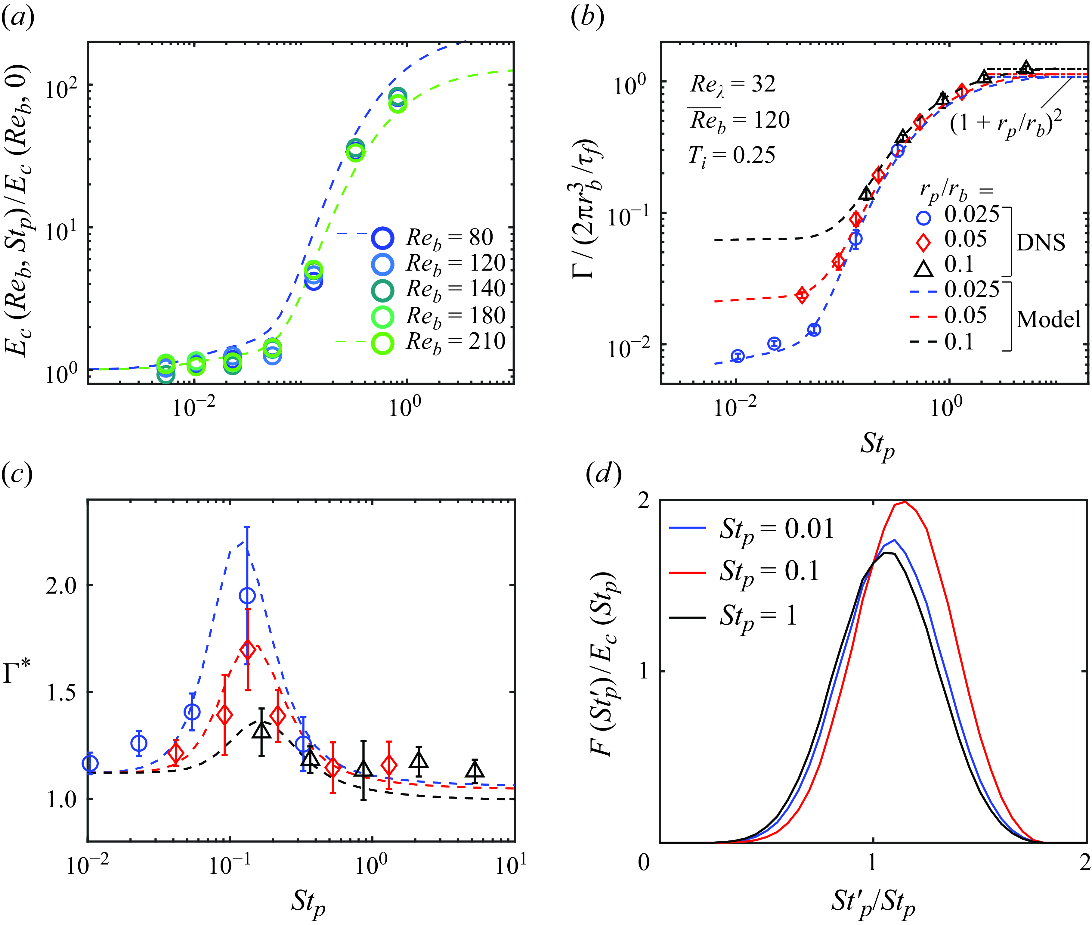
Figure 2. (a) Normalised
 $E_c$
as a function of
$E_c$
as a function of
 $St_p$
in quiescent flow for various
$St_p$
in quiescent flow for various
 $Re_b$
compared to the fits according to (4.1) (dashed lines). (b) Dimensionless collision kernel versus
$Re_b$
compared to the fits according to (4.1) (dashed lines). (b) Dimensionless collision kernel versus
 $St_p$
at
$St_p$
at
 $\overline {Re_b}=120$
for bubble with imposed velocity in HIT (symbols) and model (dashed lines). (c) Turbulent collision kernel relative to that in quiescent flow for the imposed velocity bubble. Error bars represent fluctuations between subsets of the data. (d) Scaled PDF of
$\overline {Re_b}=120$
for bubble with imposed velocity in HIT (symbols) and model (dashed lines). (c) Turbulent collision kernel relative to that in quiescent flow for the imposed velocity bubble. Error bars represent fluctuations between subsets of the data. (d) Scaled PDF of
 $St'_{p}$
as a function of
$St'_{p}$
as a function of
 $St'_{p}$
for different
$St'_{p}$
for different
 $St_p$
.
$St_p$
.
For quiescent flow, the dependence of
 $E_c$
, normalised by the result for tracer particles
$E_c$
, normalised by the result for tracer particles
 $E_c(Re_b,0)$
, on
$E_c(Re_b,0)$
, on
 $Re_b$
and
$Re_b$
and
 $St_p$
is presented in figure 2(a). For very small
$St_p$
is presented in figure 2(a). For very small
 $St_p$
, the inertial effect is negligible and the particles follow the flow streamlines, so that interception is the dominant factor determining the number of collisions in this range (Dai et al. Reference Dai, Fornasiero and Ralston2000). Analytical predictions based on flow streamlines in quiescent flow indicate that
$St_p$
, the inertial effect is negligible and the particles follow the flow streamlines, so that interception is the dominant factor determining the number of collisions in this range (Dai et al. Reference Dai, Fornasiero and Ralston2000). Analytical predictions based on flow streamlines in quiescent flow indicate that
 $\Gamma$
scales with
$\Gamma$
scales with
 $(r_p/r_b)^2$
(Weber & Paddock Reference Weber and Paddock1983) in this case. However, as particle inertia becomes more pronounced, particles deviate from the flow streamlines and collide on the bubble even if their initial position is outside the grazing trajectory of the inertialess particle. This leads to a higher collision rate and explains the rapid increase in
$(r_p/r_b)^2$
(Weber & Paddock Reference Weber and Paddock1983) in this case. However, as particle inertia becomes more pronounced, particles deviate from the flow streamlines and collide on the bubble even if their initial position is outside the grazing trajectory of the inertialess particle. This leads to a higher collision rate and explains the rapid increase in
 $E_c$
as
$E_c$
as
 $St_p$
approaches 0.1, beyond which the inertial effect dominates. At very large
$St_p$
approaches 0.1, beyond which the inertial effect dominates. At very large
 $St_p$
, the particles are barely influenced by the flow such that
$St_p$
, the particles are barely influenced by the flow such that
 $E_c$
approaches
$E_c$
approaches
 $(1+r_p/r_b)^2$
. To be able to evaluate
$(1+r_p/r_b)^2$
. To be able to evaluate
 $E_c(Re_b, St_p)$
analytically, we employ an empirical expression, which is the sum of its two contributions: interceptional collision
$E_c(Re_b, St_p)$
analytically, we employ an empirical expression, which is the sum of its two contributions: interceptional collision
 $E_i$
and the collision associated with particle inertia (Schulze Reference Schulze1989):
$E_i$
and the collision associated with particle inertia (Schulze Reference Schulze1989):
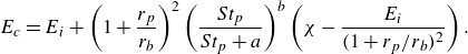 \begin{equation} E_c = E_i+\left(1+\frac {r_p}{r_b}\right)^2\left(\frac {St_p}{St_p+a}\right)^b\left(\chi -\frac {E_i}{(1+r_p/r_b)^2}\right) .\end{equation}
Here, we adopt
 $E_i=\frac {3}{2}(r_p/r_b)^2(1+Re_b^{2/3}/5)$
(Sarrot et al. Reference Sarrot, Guiraud and Legendre2005) for the collision efficiency in the tracer limit, and the fitting parameters are set to
$E_i=\frac {3}{2}(r_p/r_b)^2(1+Re_b^{2/3}/5)$
(Sarrot et al. Reference Sarrot, Guiraud and Legendre2005) for the collision efficiency in the tracer limit, and the fitting parameters are set to
 $a=0.2$
and
$a=0.2$
and
 $b=2$
. Also,
$b=2$
. Also,
 $\chi =1-0.9\times 10^{-(({\log(St)+1.3})/{1.6})^2}$
is a fitting correction term to better capture the transition around
$\chi =1-0.9\times 10^{-(({\log(St)+1.3})/{1.6})^2}$
is a fitting correction term to better capture the transition around
 $St_p\approx 0.1$
. The resulting fit is in good agreement with the data for the evaluated parameter range, as shown in figure 2(a).
$St_p\approx 0.1$
. The resulting fit is in good agreement with the data for the evaluated parameter range, as shown in figure 2(a).
As shown for the case with constant bubble velocity in figure 2(b), the general trends of
 $\Gamma$
in turbulence, in particular the increase with increasing
$\Gamma$
in turbulence, in particular the increase with increasing
 $St_p$
for all particle sizes, are consistent with those observed in quiescent flow. In this simplified configuration, the PDF of the
$St_p$
for all particle sizes, are consistent with those observed in quiescent flow. In this simplified configuration, the PDF of the
 $U'_{b}$
required to evaluate our model (2.2) can be obtained by combining the constant bubble rise velocity with the Gaussian distribution of turbulent velocity fluctuations. The collision kernel predicted in this way is in excellent agreement with the simulations. This is further confirmed in figure 2(c), where we scrutinise the result by plotting it relative to the collision kernel at the same bubble velocity in quiescent flow as
$U'_{b}$
required to evaluate our model (2.2) can be obtained by combining the constant bubble rise velocity with the Gaussian distribution of turbulent velocity fluctuations. The collision kernel predicted in this way is in excellent agreement with the simulations. This is further confirmed in figure 2(c), where we scrutinise the result by plotting it relative to the collision kernel at the same bubble velocity in quiescent flow as
 $\Gamma ^*=\Gamma /\Gamma ^q$
. In this way, it also becomes clear that turbulent flow significantly enhances the collision kernel. Here, two interesting aspects should be underscored. First,
$\Gamma ^*=\Gamma /\Gamma ^q$
. In this way, it also becomes clear that turbulent flow significantly enhances the collision kernel. Here, two interesting aspects should be underscored. First,
 $\Gamma ^*$
surpasses 1 when inertia is negligible (
$\Gamma ^*$
surpasses 1 when inertia is negligible (
 $St_p \ll 1$
), indicating that turbulent fluctuations enhance interceptional bubble-particle collision. Second, the collision enhancement is not uniform across the considered range of
$St_p \ll 1$
), indicating that turbulent fluctuations enhance interceptional bubble-particle collision. Second, the collision enhancement is not uniform across the considered range of
 $St_p$
, suggesting that the combined influence of turbulence and particle inertia leads to further amplification of the collision rate. The collision enhancement can reach approximately 100 % for particles with size ratio
$St_p$
, suggesting that the combined influence of turbulence and particle inertia leads to further amplification of the collision rate. The collision enhancement can reach approximately 100 % for particles with size ratio
 $r_p/r_b=0.025$
. For larger particles, the maximum collision enhancement is lower, though the peak still occurs at a similar value
$r_p/r_b=0.025$
. For larger particles, the maximum collision enhancement is lower, though the peak still occurs at a similar value
 $St_p\approx 0.1$
.
$St_p\approx 0.1$
.
The good agreement with the simulations indicates that the model adequately captures the relevant turbulence effects on the collisions, enabling us to explore their origin. We notice that due to the increase of
 $E_c$
with increasing
$E_c$
with increasing
 $Re'_{b}$
, the integrand in (2.2) depends nonlinearly on
$Re'_{b}$
, the integrand in (2.2) depends nonlinearly on
 $U'_{b}$
. This results in an increase in the predicted collision rate even if
$U'_{b}$
. This results in an increase in the predicted collision rate even if
 $f(U'_{b})$
is symmetric around
$f(U'_{b})$
is symmetric around
 $\overline {U_b}$
. In the present case, this effect amounts to almost a 15 % increase in
$\overline {U_b}$
. In the present case, this effect amounts to almost a 15 % increase in
 $\Gamma$
, consistent with what is observed at low
$\Gamma$
, consistent with what is observed at low
 $St_p$
.
$St_p$
.
In addition, there is an inertial effect as a change in
 $U'_{b}$
also changes
$U'_{b}$
also changes
 $St'_{p}$
. The strongly nonlinear dependence of
$St'_{p}$
. The strongly nonlinear dependence of
 $E_c$
on
$E_c$
on
 $St'_{p}$
, especially in the intermediate range
$St'_{p}$
, especially in the intermediate range
 $St_p \approx 0.1$
, leads to an asymmetric response to positive and negative velocity fluctuations. This is demonstrated by the scaled PDF of
$St_p \approx 0.1$
, leads to an asymmetric response to positive and negative velocity fluctuations. This is demonstrated by the scaled PDF of
 $St'_{p}$
,
$St'_{p}$
,
 $F(St'_{p})=E_c(St'_{p})\,PDF(St'_{p})$
, shown in figure 2(d). For low and high
$F(St'_{p})=E_c(St'_{p})\,PDF(St'_{p})$
, shown in figure 2(d). For low and high
 $St_p$
, the dependence of
$St_p$
, the dependence of
 $F(St'_{p})$
on
$F(St'_{p})$
on
 $St'_{p}$
is almost symmetric. However, for an intermediate value
$St'_{p}$
is almost symmetric. However, for an intermediate value
 $St_p\approx 0.1$
, the contribution to collisions from fluctuating
$St_p\approx 0.1$
, the contribution to collisions from fluctuating
 $St'_{p}$
exhibits a positive bias, which explains the strongly enhanced turbulent collision rate in this range, and the non-monotonic dependence on
$St'_{p}$
exhibits a positive bias, which explains the strongly enhanced turbulent collision rate in this range, and the non-monotonic dependence on
 $St_p$
. Due to the higher interceptional collision efficiency, the increase in the inertial range – and hence the turbulent enhancement – is less pronounced for larger size ratios
$St_p$
. Due to the higher interceptional collision efficiency, the increase in the inertial range – and hence the turbulent enhancement – is less pronounced for larger size ratios
 $r_p/r_b$
.
$r_p/r_b$
.
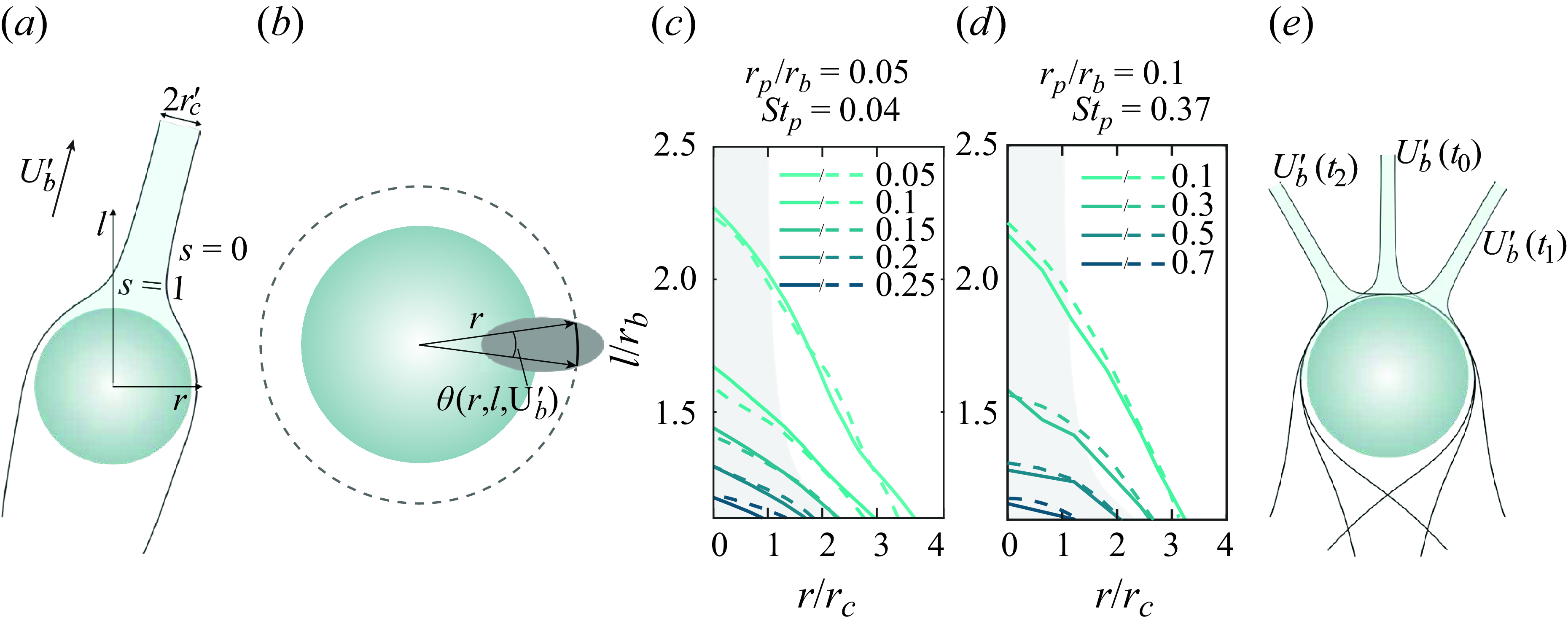
Figure 3. (a) Sketch of the bubble–particle collision with temporary slip velocity
 $\boldsymbol{U}_b'$
. The blue shaded region indicates the binary function
$\boldsymbol{U}_b'$
. The blue shaded region indicates the binary function
 $S(r,l,\boldsymbol{U}_b')$
, which is the projection of the collision tube on the
$S(r,l,\boldsymbol{U}_b')$
, which is the projection of the collision tube on the
 $r$
–
$r$
–
 $l$
plane. (b) Sketch of the cross-section (grey region) between the collision tube and the plane
$l$
plane. (b) Sketch of the cross-section (grey region) between the collision tube and the plane
 $l$
in the view along the
$l$
in the view along the
 $l$
-axis. Here,
$l$
-axis. Here,
 $\theta (r,l,\boldsymbol{U}_b')$
indicates the radian of the arc that occupied by the grey region in the circle of radius
$\theta (r,l,\boldsymbol{U}_b')$
indicates the radian of the arc that occupied by the grey region in the circle of radius
 $r$
, which is used to measure the term
$r$
, which is used to measure the term
 $G(r,l,\boldsymbol{U}_b')$
. (c,d) Contour lines of
$G(r,l,\boldsymbol{U}_b')$
. (c,d) Contour lines of
 $P(r, l)$
from simulations (solid) and model (dashed lines) for
$P(r, l)$
from simulations (solid) and model (dashed lines) for
 $(r_p/r_b=0.05,\ St_p=0.04)$
and
$(r_p/r_b=0.05,\ St_p=0.04)$
and
 $(r_p/r_b=0.1,\ St_p=0.37)$
, respectively. (e) Sketch of the collision probability under different bubble slip velocities. The region with more overlaps corresponds to the one with higher collision probability.
$(r_p/r_b=0.1,\ St_p=0.37)$
, respectively. (e) Sketch of the collision probability under different bubble slip velocities. The region with more overlaps corresponds to the one with higher collision probability.
Another way to validate the model is to consider the spatial distribution of the collision probability
 $P(r,\ l)$
, where
$P(r,\ l)$
, where
 $r$
and
$r$
and
 $l$
are distances perpendicular to and along the bubble velocity direction, respectively (see figure 3
a). In quiescent flow, the collision process is deterministic and the collisions probability is a binary function, which has a tube shape based on the grazing trajectory (see the shaded region in figure 3
a). We represent this using the binary function
$l$
are distances perpendicular to and along the bubble velocity direction, respectively (see figure 3
a). In quiescent flow, the collision process is deterministic and the collisions probability is a binary function, which has a tube shape based on the grazing trajectory (see the shaded region in figure 3
a). We represent this using the binary function
 $S(r,l;\boldsymbol{U}_b)$
, which is equal to 1 inside the collision tube, and 0 otherwise, as shown in figure 3(a). Practically,
$S(r,l;\boldsymbol{U}_b)$
, which is equal to 1 inside the collision tube, and 0 otherwise, as shown in figure 3(a). Practically,
 $S$
can be determined from the grazing trajectory. Based on the ‘frozen turbulence’ assumption, the collision probability in turbulence can be predicted as the superposition of the binary probability distributions corresponding to the instantaneous slip velocity
$S$
can be determined from the grazing trajectory. Based on the ‘frozen turbulence’ assumption, the collision probability in turbulence can be predicted as the superposition of the binary probability distributions corresponding to the instantaneous slip velocity
 $\boldsymbol{U}_b'$
. This leads to
$\boldsymbol{U}_b'$
. This leads to
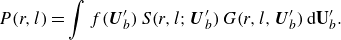 \begin{equation} P(r,l) = \int f(\boldsymbol{U}_b')\,S(r,l;\boldsymbol{U}_b')\,G(r,l,\boldsymbol{U}_b')\,\textrm {d}\mathbf {U}_b'. \end{equation}
Note that the additional factor
 $G(r,l,\boldsymbol{U}_b')=\theta (r,l,\boldsymbol{U}_b')/2\pi$
in (4.2) is a geometrical coefficient related to the azimuthal integration required for the projection onto the two-dimensional
$G(r,l,\boldsymbol{U}_b')=\theta (r,l,\boldsymbol{U}_b')/2\pi$
in (4.2) is a geometrical coefficient related to the azimuthal integration required for the projection onto the two-dimensional
 $(r,l)$
space. It measures the fraction of the circle with radius
$(r,l)$
space. It measures the fraction of the circle with radius
 $r$
that falls inside the collision tube at distance
$r$
that falls inside the collision tube at distance
 $l$
, as illustrated in figure 3(b). The result of the model prediction according to (4.2) is again in excellent agreement with the data as shown in figures 3(c) and 3(d), confirming that the basic physical processes are well represented in the model. Consistent with figure 1(d), the impact of turbulence is clearly evident, leading to a much wider distribution of
$l$
, as illustrated in figure 3(b). The result of the model prediction according to (4.2) is again in excellent agreement with the data as shown in figures 3(c) and 3(d), confirming that the basic physical processes are well represented in the model. Consistent with figure 1(d), the impact of turbulence is clearly evident, leading to a much wider distribution of
 $P(r,\ l)$
compared to the binary distribution in quiescent flow. This effect is especially pronounced if
$P(r,\ l)$
compared to the binary distribution in quiescent flow. This effect is especially pronounced if
 $St_p$
is low, as is the case for figure 3(c). The collision efficiency is low, and the associated collision stream tube is slender for this case, such that fluctuations in the instantaneous bubble slip direction lead to low values of
$St_p$
is low, as is the case for figure 3(c). The collision efficiency is low, and the associated collision stream tube is slender for this case, such that fluctuations in the instantaneous bubble slip direction lead to low values of
 $P(r,\ l)$
even close to the bubble surface, as is illustrated in figure 3(e). Since the collision efficiency increases for larger
$P(r,\ l)$
even close to the bubble surface, as is illustrated in figure 3(e). Since the collision efficiency increases for larger
 $St_p$
and the collision tube widens, this effect becomes less strong, and the values of the collision probability close to the bubble are much higher in the plot for
$St_p$
and the collision tube widens, this effect becomes less strong, and the values of the collision probability close to the bubble are much higher in the plot for
 $St_p = 0.37$
in figure 3(d).
$St_p = 0.37$
in figure 3(d).

Figure 4. Normalised collision kernel for the freely rising bubble at (a)
 $Re_\lambda =32$
,
$Re_\lambda =32$
,
 $\overline {Re_b}=110$
and (b)
$\overline {Re_b}=110$
and (b)
 $Re_\lambda =64$
,
$Re_\lambda =64$
,
 $\overline {Re_b}=150$
. (c) Comparison of auto-correlation function of
$\overline {Re_b}=150$
. (c) Comparison of auto-correlation function of
 $U'_{b}$
for the imposed velocity (
$U'_{b}$
for the imposed velocity (
 $Re_\lambda =32,\ \overline {Re_b}=120$
) and freely rising bubbles (
$Re_\lambda =32,\ \overline {Re_b}=120$
) and freely rising bubbles (
 $Re_\lambda =32,\ \overline {Re_b}=110$
), respectively. (d) The normalised mean incoming particle number density as a function of
$Re_\lambda =32,\ \overline {Re_b}=110$
), respectively. (d) The normalised mean incoming particle number density as a function of
 $St_p$
at
$St_p$
at
 $Re_\lambda =64$
. (e) Sketch in the bubble reference frame, showing how fluctuations
$Re_\lambda =64$
. (e) Sketch in the bubble reference frame, showing how fluctuations
 $U'_{b}$
during the interaction effectively enlarge the particle collision radius.
$U'_{b}$
during the interaction effectively enlarge the particle collision radius.
Having established the general suitability of the model to capture the relevant turbulence effects on the collision rate, we now turn to the more realistic case of a freely rising bubble. The corresponding results in terms of
 $\Gamma$
are shown in figures 4(a,b) for different
$\Gamma$
are shown in figures 4(a,b) for different
 $Re_\lambda$
. In these cases, the bubble slip velocity PDF
$Re_\lambda$
. In these cases, the bubble slip velocity PDF
 $f(U'_{b})$
required as input for the model is measured by averaging the fluid velocity located on a spherical surface of radius
$f(U'_{b})$
required as input for the model is measured by averaging the fluid velocity located on a spherical surface of radius
 $3r_b$
that is centred at the bubble’s centre position (Kidanemariam et al. Reference Kidanemariam, Clemens, Doychev and Uhlmann2013). The size of the spherical surface is chosen in a way such that the fluid velocity is not significantly influenced by the presence of the bubble boundary. The radius
$3r_b$
that is centred at the bubble’s centre position (Kidanemariam et al. Reference Kidanemariam, Clemens, Doychev and Uhlmann2013). The size of the spherical surface is chosen in a way such that the fluid velocity is not significantly influenced by the presence of the bubble boundary. The radius
 $3r_b$
of the spherical surface is tested in the case of uniform flow past a fixed sphere (Kidanemariam et al. Reference Kidanemariam, Clemens, Doychev and Uhlmann2013), which results in a measured fluid velocity corresponding to approximately
$3r_b$
of the spherical surface is tested in the case of uniform flow past a fixed sphere (Kidanemariam et al. Reference Kidanemariam, Clemens, Doychev and Uhlmann2013), which results in a measured fluid velocity corresponding to approximately
 $90\,\%$
of the incoming flow velocity.
$90\,\%$
of the incoming flow velocity.
The general agreement between
 $\Gamma$
predicted by the model (dashed lines in figures 4
a,b) and the data remains good also for the free rising cases. Difference arises at low
$\Gamma$
predicted by the model (dashed lines in figures 4
a,b) and the data remains good also for the free rising cases. Difference arises at low
 $St_p$
, where the model is found to underpredict the simulation result. This can be explained by the correlation time of
$St_p$
, where the model is found to underpredict the simulation result. This can be explained by the correlation time of
 $U'_{b}$
, which is shorter for free rising bubbles compared to the imposed velocity case (see figure 4
c). The resulting changes in
$U'_{b}$
, which is shorter for free rising bubbles compared to the imposed velocity case (see figure 4
c). The resulting changes in
 $U'_{b}$
during the bubble–particle interaction cause the particle trajectory to fluctuate in the bubble frame of reference (see the sketch in figure 4
e). This increases the effective collision radius of the particle to
$U'_{b}$
during the bubble–particle interaction cause the particle trajectory to fluctuate in the bubble frame of reference (see the sketch in figure 4
e). This increases the effective collision radius of the particle to
 $r_p+d$
, where
$r_p+d$
, where
 $d$
is a measure of the drift from the original particle trajectory. The relevant time and velocity scales for this drift are
$d$
is a measure of the drift from the original particle trajectory. The relevant time and velocity scales for this drift are
 $\tau _f$
and
$\tau _f$
and
 $u_\eta$
, respectively, such that
$u_\eta$
, respectively, such that
 $d \sim \tau _f u_\eta$
in analogy to Taylor dispersion in the ballistic regime (Taylor Reference Taylor1922). Indeed, we find that using
$d \sim \tau _f u_\eta$
in analogy to Taylor dispersion in the ballistic regime (Taylor Reference Taylor1922). Indeed, we find that using
 $d = 0.06\tau _f u_\eta$
results in good agreement with our data across different
$d = 0.06\tau _f u_\eta$
results in good agreement with our data across different
 $Re_\lambda$
and for different
$Re_\lambda$
and for different
 $r_p$
, as shown by the dash-dotted lines in figures 4(a,b). This effect is relevant only at
$r_p$
, as shown by the dash-dotted lines in figures 4(a,b). This effect is relevant only at
 $St_p \lessapprox 0.1$
, and becomes negligible once
$St_p \lessapprox 0.1$
, and becomes negligible once
 $r_c\gg d$
due to the inertial effect at larger
$r_c\gg d$
due to the inertial effect at larger
 $St_p$
.
$St_p$
.
Another finding is that the incoming particle number density can differ from the global value. This is caused by clustering of bubbles and particles in different regions of the flow, leading to segregation (Chan et al. Reference Chan, Ng and Krug2023). As a result,
 $\langle n'_{p}\rangle /n_p$
shown in figure 4(d) decreases as
$\langle n'_{p}\rangle /n_p$
shown in figure 4(d) decreases as
 $St_p$
increases, reaching minimum value of approximately 0.8 for
$St_p$
increases, reaching minimum value of approximately 0.8 for
 $St_p \approx 1$
, where clustering effects are known to be strongest. The segregation effect explains why the inertial limit
$St_p \approx 1$
, where clustering effects are known to be strongest. The segregation effect explains why the inertial limit
 $(1+r_p/r_b)^2$
at high
$(1+r_p/r_b)^2$
at high
 $St_p$
is not reached in the simulations and in the model, where this effect is accounted for by multiplying with the factor
$St_p$
is not reached in the simulations and in the model, where this effect is accounted for by multiplying with the factor
 $\langle n'_{p}\rangle /n_p$
obtained from the simulations.
$\langle n'_{p}\rangle /n_p$
obtained from the simulations.
5. Conclusions
We have elucidated the relevant mechanisms governing the collision rate of inertial particles with a finite-size bubble in turbulence. We demonstrated that for the investigated practical conditions, inertial effects induced by the flow around the bubble are the dominant effect. The nonlinear dependence of these effects on the bubble slip velocity leads to an increase of the collision rate in turbulence of up to 100 % at
 $St_p \approx 0.1$
compared to quiescent flow. An additional increase in the turbulent collision rate is due to the short temporal correlation of the bubble slip velocity in the free-rising case. The effect of the resulting fluctuations during the bubble–particle interaction can be captured by an increase in the effective collision radius of the particle, and is mostly relevant in the tracer limit for
$St_p \approx 0.1$
compared to quiescent flow. An additional increase in the turbulent collision rate is due to the short temporal correlation of the bubble slip velocity in the free-rising case. The effect of the resulting fluctuations during the bubble–particle interaction can be captured by an increase in the effective collision radius of the particle, and is mostly relevant in the tracer limit for
 $St_p\lessapprox 0.1$
. Segregation of bubbles and particles in turbulence reduces the particle density encountered by the bubble and hence the collision rate by up to 20 % at
$St_p\lessapprox 0.1$
. Segregation of bubbles and particles in turbulence reduces the particle density encountered by the bubble and hence the collision rate by up to 20 % at
 $St_p\approx 1$
. Remarkably, the effect of turbulence-induced motion of the particles was found to have negligible impact during the transient bubble–particle interaction, whereas the incoming particle number density is reduced for particles with large Stokes number. The developed frozen turbulence model provides a physically consistent framework that can be easily extended to a full collision model (by combining it with a prediction for
$St_p\approx 1$
. Remarkably, the effect of turbulence-induced motion of the particles was found to have negligible impact during the transient bubble–particle interaction, whereas the incoming particle number density is reduced for particles with large Stokes number. The developed frozen turbulence model provides a physically consistent framework that can be easily extended to a full collision model (by combining it with a prediction for
 $f(U'_{b})$
). The approach is also transferable to other conditions, such as more complex shapes (by adopting a different parametrisation of
$f(U'_{b})$
). The approach is also transferable to other conditions, such as more complex shapes (by adopting a different parametrisation of
 $E_c$
), and thus offers a more general relevance for collisions with finite-size objects in turbulence.
$E_c$
), and thus offers a more general relevance for collisions with finite-size objects in turbulence.
Supplementary movie
Supplementary movie is available at https://doi.org/10.1017/jfm.2025.44.
Acknowledgements
We thank Timothy Chan and Duco van Buuren for fruitful discussions. This project has received funding from the European Research Council (ERC) under the European Union’s Horizon 2020 research and innovation programme (grant agreement no. 950111, BU-PACT). This work was carried out on the Dutch national e-infrastructure with the support of SURF Cooperative.
Declaration of interests
The authors report no conflict of interest.
Appendix A
As we observe that the trajectories of collided particles in HIT are significantly different from those in quiescent flow, it is interesting to study how turbulence affects the collision angle. In figure 5, we investigate the collision angle
 $\theta$
for the case where the bubble velocity is imposed. Here,
$\theta$
for the case where the bubble velocity is imposed. Here,
 $\theta$
denotes the angle between the direction of the imposed bubble velocity and the vector of collision position in the bubble frame. We observe that the mean collision angle
$\theta$
denotes the angle between the direction of the imposed bubble velocity and the vector of collision position in the bubble frame. We observe that the mean collision angle
 $\langle \theta \rangle$
for the turbulence flow is higher than that for the case of quiescent flow. However,
$\langle \theta \rangle$
for the turbulence flow is higher than that for the case of quiescent flow. However,
 $\langle \theta \rangle$
shows a similar dependence on
$\langle \theta \rangle$
shows a similar dependence on
 $St_p$
for both cases, where
$St_p$
for both cases, where
 $\langle \theta \rangle$
first decreases as
$\langle \theta \rangle$
first decreases as
 $St_p$
, and rises after. This can be explained by inertial effects on the particles as illustrated in figures 5(b) and 5(c) for the deterministic case. At low
$St_p$
, and rises after. This can be explained by inertial effects on the particles as illustrated in figures 5(b) and 5(c) for the deterministic case. At low
 $St_p$
,
$St_p$
,
 $r_c$
is small. Consequently, particles collide on the bubble front region, where the streamlines are strongly curved. Therefore, particle trajectories deviate significantly from the streamlines as
$r_c$
is small. Consequently, particles collide on the bubble front region, where the streamlines are strongly curved. Therefore, particle trajectories deviate significantly from the streamlines as
 $St_p$
increases. As a consequence, higher-inertia particles collide at a smaller collision angle, as illustrated in figure 5(b). When
$St_p$
increases. As a consequence, higher-inertia particles collide at a smaller collision angle, as illustrated in figure 5(b). When
 $St_p$
surpasses the critical value,
$St_p$
surpasses the critical value,
 $r_c$
becomes larger. In this case, increasing particle inertia leads to a higher collision rate as well as to a higher collision angle, which is illustrated in figure 5(c). These general trends for
$r_c$
becomes larger. In this case, increasing particle inertia leads to a higher collision rate as well as to a higher collision angle, which is illustrated in figure 5(c). These general trends for
 $\langle \theta \rangle$
are retained in the turbulent case, which is in line with our approach of representing the instantaneous collision process by the deterministic case. Figures 5(d–f) show the scaled PDF of collision angle
$\langle \theta \rangle$
are retained in the turbulent case, which is in line with our approach of representing the instantaneous collision process by the deterministic case. Figures 5(d–f) show the scaled PDF of collision angle
 $\theta$
for different particle sizes. The scaled PDF illustrates the distribution of the collision angle, as well as where the collision differences occur between HIT and quiescent flow. The distributions of collision angle indicate that the collisions are more likely to take place at intermediate angles. Moreover, we observe that the distribution extends to a wider range in HIT, and more collisions occur, which is consistent with the observations for
$\theta$
for different particle sizes. The scaled PDF illustrates the distribution of the collision angle, as well as where the collision differences occur between HIT and quiescent flow. The distributions of collision angle indicate that the collisions are more likely to take place at intermediate angles. Moreover, we observe that the distribution extends to a wider range in HIT, and more collisions occur, which is consistent with the observations for
 $\langle \theta \rangle$
.
$\langle \theta \rangle$
.
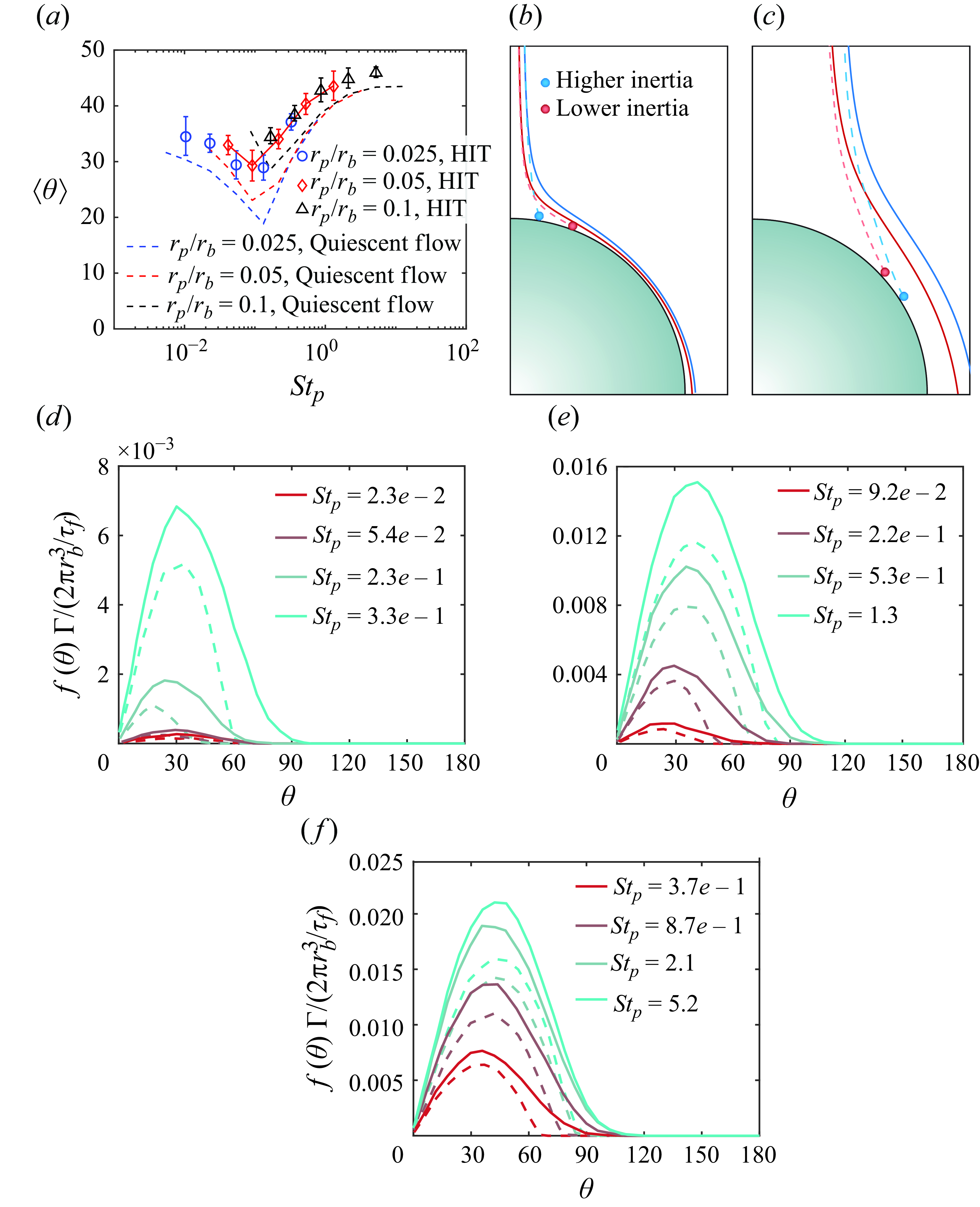
Figure 5. (a) Mean collision angle
 $\langle \theta \rangle$
as a function of
$\langle \theta \rangle$
as a function of
 $St_p$
. (b,c) Sketches illustrate the mechanism that
$St_p$
. (b,c) Sketches illustrate the mechanism that
 $\langle \theta \rangle$
declines/increases as increasing inertia when
$\langle \theta \rangle$
declines/increases as increasing inertia when
 $St_p$
is low/large in quiescent flow. The solid lines denote the streamlines along which the particles originally stay, and the dashed lines are the particle trajectories. (d–f) The PDFs of collision angle
$St_p$
is low/large in quiescent flow. The solid lines denote the streamlines along which the particles originally stay, and the dashed lines are the particle trajectories. (d–f) The PDFs of collision angle
 $f(\theta )$
scaled by the normalised collision kernel for particle size
$f(\theta )$
scaled by the normalised collision kernel for particle size
 $r_p/r_b=0.025,0.05,0.1$
in HIT (solid lines) and quiescent flow (dashed lines).
$r_p/r_b=0.025,0.05,0.1$
in HIT (solid lines) and quiescent flow (dashed lines).


 Open access