


1. Introduction
A question central to the study of flight is the effect of flow unsteadiness on energy consumption. Range and endurance limit the utility of flight vehicles, particularly small ones (Wood Reference Wood2007; Chabot Reference Chabot2018; Shakhatreh et al. Reference Shakhatreh, Sawalmeh, Al-Fuqaha, Dou, Almaita, Khalil, Othman, Khreishah and Guizani2019). While it is common to make predictions of range and endurance under the assumption that the air is quiescent, this assumption can be inaccurate. Given a specific trajectory, flight through unsteady air comes at the expense of the work performed to maintain the trajectory. Perhaps the unsteadiness, or turbulence, can itself be so energetic that it represents an auxiliary energy reservoir that can be used to maintain flight. The challenge is to show if and when the latter case can prevail. Related questions apply to volant lifeforms (Norberg Reference Norberg1996; Bowlin & Wikelski Reference Bowlin and Wikelski2008).
It is well known that energy can be extracted from mean winds and large coherent structures in the atmosphere in order to extend range or endurance. Examples include thermal updrafts, mountain waves and shear layers. These structures are approximately steady and predictable enough to be exploited by glider pilots (de Divitiis Reference de Divitiis2002; Teets & Carter Reference Teets and Carter2002; Langelaan Reference Langelaan2007; Chudej, Klingler & Britzelmeier Reference Chudej, Klingler and Britzelmeier2015), birds (Ákos et al. Reference Ákos, Nagy, Leven and Vicsek2010; Nourani & Yamaguchi Reference Nourani and Yamaguchi2017) and autonomous flight vehicles (White et al. Reference White, Watkins, Lim and Massey2012; Fisher et al. Reference Fisher, Marino, Clothier, Watkins, Peters and Palmer2015; Watkins et al. Reference Watkins, Mohamed, Fisher, Clothier, Carrese and Fletcher2015; Reddy et al. Reference Reddy, Celani, Sejnowski and Vergassola2016).
Energy can also be extracted from the atmosphere when there is no mean wind by responding in specific ways to random gusts, or turbulent fluctuations. Birds such as the albatross may do so (Pennycuick Reference Pennycuick2002, Reference Pennycuick2008; Mallon, Bildstein & Katzner Reference Mallon, Bildstein and Katzner2015). The majority of autonomous methods developed by humans to do so respond to flow measurements (Patel & Kroo Reference Patel and Kroo2006; Lissaman & Patel Reference Lissaman and Patel2007; Langelaan & Bramesfeld Reference Langelaan and Bramesfeld2008), while birds or glider pilots may instead respond to their own accelerations (Morelli Reference Morelli2003; Laurent et al. Reference Laurent, Fogg, Ginsburg, Halverson, Lanzone, Miller, Winkler and Bewley2021). Quinn et al. (Reference Quinn, Kress, Chang, Stein, Wegrzynski and Lentink2019) show that birds responded effectively to unsteady flows given even limited sensory information. Katzmayr (Reference Katzmayr1922) shows that fixed-wing aircraft can extract the energy in random gusts by clever transient rotations of the net aerodynamic force vector. To understand the effect, which Patel, Lee & Kroo (Reference Patel, Lee and Kroo2009) verify in flight, consider that fixed-wing aircraft generally have much greater lift than drag so that their combination, or the net aerodynamic force on the aircraft, is almost normal to the direction of motion. Consequently, small upward gusts rotate the direction of the mean flow slightly in the reference frame of the wing and tilt the aerodynamic force forward transiently, which reduces drag (or increases thrust). Ignoring mean winds, upward and downward gusts are equally likely, but due to a nonlinearity the upward gusts cause larger net aerodynamic forces, so that transient drag reductions from upward gusts outweigh the corresponding increases from downward gusts. While gust velocities are smaller than the cruise speed of most aircraft, they are often of the same order as the downwash velocity so that vertical gusts can induce a significant change in the orientation of the lift vector relative to the aircraft's direction of flight, enough to cause flight power to drop transiently and even vanish (Pennycuick Reference Pennycuick2002; Lissaman & Patel Reference Lissaman and Patel2007). This makes vertical gust energy extraction effective for birds and fixed-wing aircraft. For rotorcraft, in contrast, the downwash velocity is typically large compared with vertical gust velocities so that flight power is not strongly affected. Neutrally buoyant vehicles do not require energy to maintain altitude (or depth for submarines) so that they cannot exploit the Katzmayr effect.
The methods developed for fixed-wing aircraft as well as those employed by birds and glider pilots appear to have in common a tendency to amplify gust disturbances, in specific and controlled ways, rather than suppress them – the opposite of what is typical in stability and control problems (Morelli Reference Morelli2003; Patel et al. Reference Patel, Lee and Kroo2009; Mallon et al. Reference Mallon, Bildstein and Katzner2015). Gorisch (Reference Gorisch2011) notes that reducing glider inertia as well as adding positive feedback flaps to increase gust-induced accelerations can theoretically improve turbulent energy capture.
Most algorithms for fixed-wing aircraft rely on the Katzmayr effect and the oversampling of flow in upwards gusts to extract energy from the gusts. Hence, these methods take a time-based signals approach to turbulence in the sense that the only necessary information about the flow is the vertical gust velocity as a function of time. The methods do not incorporate knowledge about the spatial structure of the flow. Rather than taking this approach, which results in appreciable benefits only for fixed-wing aircraft utilizing vertical gusts, gust energy capture has also been framed as a global path optimization problem. Given known wind fields, flight paths are routinely optimized to avoid headwinds and seek out tailwinds. With full knowledge of the flow, it is also possible to avoid downdrafts and seek out updrafts. These ideas apply underwater and on free surfaces as well, and are similar in spirit to updraft, thermal, and shear-layer soaring in that they typically only apply when flows are approximately stationary (Langelaan Reference Langelaan2007; Fernández-Perdomo et al. Reference Fernández-Perdomo, Cabrera, Hernández-Sosa, Isern, Domínguez-Brito, Redondo, Coca, Ramos, Alvarez Fanjul and Garcia2010; Yokoyama Reference Yokoyama2011; Koay & Chitre Reference Koay and Chitre2013; Chudej et al. Reference Chudej, Klingler and Britzelmeier2015; Mahmoudzadeh, Powers & Yazdani Reference Mahmoudzadeh, Powers and Yazdani2016). The global approach to path optimization through turbulence is challenging because it requires rapidly updated flow-field measurements or real-time modelling and prediction of the flow. Furthermore, methods and algorithms employed at present on autonomous vehicles are often limited by the measurements the vehicle can itself make about its environment (e.g. Garau, Alvarez & Oliver Reference Garau, Alvarez and Oliver2006).
In this paper we address the global path optimization problem using fluid dynamics to find efficient yet sub-optimal paths through turbulence without the need for real-time optimization algorithms. We analyse, theoretically, a way for vehicles to extract energy from turbulence by mimicking the aerodynamic coupling between inertial particles and turbulence. Inertial particles falling through turbulence naturally find non-trivial and energetically favourable paths that vehicles can follow using information only about their own accelerations, with no real-time modelling, and with only a parametric description of the flow. To see how this is possible requires an understanding of the way inertial particles behave in turbulence when gravity biases their direction of motion.
Small particles fall down through turbulent flows faster on average than through a quiescent fluid; in some cases, nearly three times faster (Maxey Reference Maxey1987a,Reference Maxeyb; Wang & Maxey Reference Wang and Maxey1993; Good et al. Reference Good, Ireland, Bewley, Bodenschatz, Collins and Warhaft2014; Tom & Bragg Reference Tom and Bragg2019). Although completely passive, particles find these favourable paths when their inertial time scale is resonant with a flow time scale, or in flows that evolve approximately as quickly as the particles can respond to this evolution. Under these conditions, particles tend to be swept toward the sides of vortices that push them down more quickly (Wang & Maxey Reference Wang and Maxey1993).
Rotorcraft, or any other vehicle, forced to act like particles of the right inertia can passively find faster paths, albeit in the direction of their destination rather than toward the ground. To do so, a vehicle needs to apply forces proportional to its measured instantaneous accelerations, for instance, and thereby modify its effective mass so that it reacts to gusts just as fast-tracking particles do, but with a bias toward a destination provided by a mean thrust rather than by gravity. This results in energy extraction from turbulence in spite of a lack of knowledge about the instantaneous structure of the surrounding flow. It is a proof of this principle that we explore in this paper.
We call the forcing cyber-physical since it changes the effective inertia of the rotorcraft. The concept of using cyber-physical tools to achieve desired interactions between a body and flow has been explored before. Mackowski & Williamson (Reference Mackowski and Williamson2011), for instance, study fluid–structure interactions and vortex shedding on a cylinder. Previous implementations rely on tethered force measurements rather than untethered acceleration measurements in their computations (Hover, Techet & Triantafyllou Reference Hover, Techet and Triantafyllou1998; Mackowski & Williamson Reference Mackowski and Williamson2011).
We focus in this paper primarily on rotorcraft that are smaller than the size of the dominant turbulent flow structures through which they fly, and that move in only two dimensions, one of which is in the direction of a destination. The two dimensions are perpendicular to gravity, with a mean thrust for rotorcraft playing the role of gravity for inertial particles.
In § 2, we review a simple model of rotorcraft flight and propose a simple cyber-physical forcing on the rotorcraft. We find that the form of the dimensionless equations of motion is the same as the one for settling particles. The forcing allows rotorcraft to mimic a particle of any settling parameter and Stokes number. While the forcing allows any place in parameter space to be reached in principle, there is a cost to doing so determined by the magnitude of the forces the rotorcraft needs to generate in order to mimic the desired particle dynamics. We find that these costs are determined in part by the moments of the probability density function of inertial-particle accelerations. The balance between the costs and the gains realized by moving into energetically favourable parts of parameter space lead to the existence of optimal shifts in the parameters, which depend on the characteristics of the turbulence and of the rotorcraft in ways that we calculate. The methods section (§ 3) describes how we simulated turbulence, rotorcraft flight, and how we perform the optimizations.
In § 4 we present the advantages realized by a simple cyber-physical forcing. The purpose of the calculations is to delineate the boundaries in parameter space within which potential gains can be realized by the forcing. We find that compared with flight through quiescent fluid (QF), fast-tracking forcing (FT) reduces both energy consumption and flight time. The advantages are significant for rotorcraft with natural response times faster than the characteristic turnover time of the flow, and for vehicles with cruising speeds within an order of magnitude of the characteristic speed of turbulent fluctuations in the flow. Relative to doing nothing (DN), in a sense explained below, the advantage of the forcing is to broaden the range of conditions under which turbulence benefits flight, particularly if the effective vehicle inertia is anisotropic as explained in the theory section. DN in turbulence is automatically beneficial relative to flight through QF due to intrinsic fast-tracking, provided the relevant dynamics applies or can be made to apply to a vehicle. The cost of gust suppression, or disturbance rejection (DR), is large compared with the gains realized by any other flight mode.
We expect that further benefits to flight may be realized through increased sophistication of the forcing model, ideas for which we review in § 5. Furthermore, comparisons with experiments on particles in turbulence suggest gains up to ten times larger than those we found in our calculations (Wang & Maxey Reference Wang and Maxey1993; Good et al. Reference Good, Ireland, Bewley, Bodenschatz, Collins and Warhaft2014). The reduced gains appearing in the calculations are comparable to those achieved in previous studies using turbulence models that respect turbulence statistics and kinematics but ignore the dynamics of real turbulence. This may be the result of vorticity in the models not being as strongly correlated spatially or temporally as in real turbulence. Finally, we believe that the theory can be generalized to three dimensions and to any properly forced vehicle moving in a turbulent fluid.
2. Theory
As a foundation for autonomous flight strategies to navigate turbulent flows efficiently, we use a simple model of flight vehicle dynamics to show how it leads naturally to a forcing strategy. The flight vehicle is a rotorcraft, meaning that the thrust not only propels the vehicle but also directly supports its weight. One component of the thrust points in a fixed direction, meaning that the destination for the flight vehicle is at  $\infty$, or far away. We consider statistically homogeneous, isotropic turbulence with a zero mean, and for further simplicity, we consider flows that fluctuate only in the plane perpendicular to gravity. Fast tracking operates in both two and three dimensions, and we expect the results we observe in two dimensions to generalize to three (Maxey & Corrsin Reference Maxey and Corrsin1986; Rosa et al. Reference Rosa, Parishani, Ayala and Wang2016). The potential advantages are realized statistically, meaning that our results are expectation values for many flights, or for long flights, through statistically stationary turbulent flows.
We compare the case of flight through turbulence under FT forcing to the cases of flight through each of quiescent fluid (QF), turbulent fluid while DN, and turbulent fluid while rejecting disturbances. The letters in parentheses appear as subscripts to denote the conditions under which different quantities were calculated. While the DN case does not correct deviations from its path caused by turbulence, implicit in all cases is the assumption that the rotorcraft controls its angular degrees of freedom quickly compared to the dynamics of interest; this may be a better assumption for rotorcraft than for fixed-wing aircraft in turbulence (Watkins et al. Reference Watkins, Abdulrahim, Thompson, Shortis, Loxton, Segal, Bil and Watmuff2012).
2.1. Particle dynamics and fast tracking
The momentum equation for heavy particles balances the particle's inertia with drag and gravity and is
 \begin{equation} \frac{\textrm{d}\tilde{\boldsymbol{u}}}{\textrm{d}\tilde{t}} = \tilde{\boldsymbol{f}}_{d,p} + \tilde{\boldsymbol{g}}, \end{equation}
where  $\tilde {\boldsymbol {u}}$ is the particle velocity, tildes denote quantities with units and the coordinate system is in figure 1. Additional terms are needed to capture non-zero Reynolds-number and fluid-inertia effects, which we neglect since the dynamics produced by (2.1) captures the inertial-particle phenomena of interest here (Maxey & Riley Reference Maxey and Riley1983).

Figure 1. Movement is in the  $\hat {\boldsymbol {e}}_1$–
 $\hat {\boldsymbol {e}}_2$ plane (red), while gravity (
 ${\boldsymbol {g}}$) points in the
  $-\hat {\boldsymbol {e}}_3$ direction. The constant component of the thrust,
  ${\boldsymbol {f}}_0$, points opposite to
  $\hat {\boldsymbol {e}}_2$, and additional components defined in the text include the one given by the forcing,
  ${\boldsymbol {f}}_C$. Drag on the vehicle,
  ${\boldsymbol {f}}_d$, depends on the relative velocity between the vehicle and fluid.
Drag on small particles is linear in the velocity relative to the fluid, and the specific drag force is
 \begin{equation} \tilde{\boldsymbol{f}}_{d,p} = (\tilde{\boldsymbol{w}}-\tilde{\boldsymbol{u}})/\tau_p, \end{equation}
where  $\tau _p$ is the characteristic response time of the particle and is large for massive, inertial particles. For particles at low Reynolds numbers,
  $\tau _p$ is given by Stokes’ law,
  $\tau _p = \rho d^{2}/18\mu$, where
  $\rho$ and
  $\mu$ are the density and viscosity of the fluid, and
  $d$ is the diameter of the particle (e.g. Wang & Maxey Reference Wang and Maxey1993). The fluctuating fluid velocity in the vicinity of the particle is
  $\tilde {\boldsymbol {w}}$, which is not modified by the presence of the particle in this model, and is given by measurements or by solutions to the Navier–Stokes equations for the fluid. We let
  $\tilde {\boldsymbol {g}} = -\tilde {g}\hat {\boldsymbol {e}}_3$, as in figure 1, and we do not model the particle orientation (Maxey & Riley Reference Maxey and Riley1983).
We make (2.1) dimensionless with the characteristic velocity and length scales of the turbulence,  $U$ and
  $L$, respectively, and incorporate (2.2) so that
 \begin{equation} \frac{\textrm{d}\boldsymbol{u}}{\textrm{d}t} = \frac{1}{St_{p}}(\boldsymbol{w} - \boldsymbol{u} - W_p\hat{\boldsymbol{e}}_3), \end{equation}
where the Stokes number,  $St_p = \tau _pU/L$, compares the characteristic turbulence and particle time scales and is large for heavy particles, and the settling parameter
  $W_p = U_{QF,p}/U$ is the ratio of the particle's settling velocity through quiescent fluid,
  $U_{QF,p} = \tau _p g$, to the characteristic velocity of the turbulence. In general, the perturbations caused by turbulence lead to increased path lengths for particles settling through the fluid. Intuition may suggest, then, that settling times generally increase through turbulent fluid relative to quiescent fluid, but this is not the case.
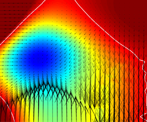
An interesting feature of solutions to (2.3) is that the mean particle velocity (in the direction of  ${\boldsymbol {g}}$), is larger in a turbulent flow than in a QF (Maxey Reference Maxey1987a). The surface of mean settling velocity, which depends on
  $St_p$ and
  $W_p$, has a basin of increased velocity as its single feature of interest. This basin is centred near normalized particle inertia and velocity of order one. The phenomenon, called fast tracking (Maxey & Corrsin Reference Maxey and Corrsin1986), occurs despite path lengths being increased by turbulence. An eddy moving opposite a particle's direction of motion tends to push the particle away, causing the particle to move into a new eddy. On the other hand, eddies with the same direction of motion as the particle sweep the particle along. In this way, particles tend to be swept into those parts of a turbulent flow with tailwinds without need for sensors or computation.
In the following sections we define and characterize a cyber-physical forcing designed to produce FT in flight vehicles even if a vehicle's inertia and air speed are not appropriately tuned with the flow in the way that produces fast tracking in particles.
2.2. Flight vehicle dynamics (DN)
In order to generate qualitative insight, we treat flight vehicles theoretically like small particles characterized only by their mass, by a drag force proportional to their motion relative to air, and by a body force. For small particles, the body force is gravity, while for flight vehicles it is the thrust that keeps them aloft and propels them toward a given destination. While this model ignores many important aspects of flight vehicle dynamics (e.g. Johnson Reference Johnson1980), it is commonly used for rotorcraft and fixed-wing flight control problems both with and without turbulence (e.g. Patel et al. Reference Patel, Lee and Kroo2009; Kushleyev et al. Reference Kushleyev, Mellinger, Powers and Kumar2013; Preiss et al. Reference Preiss, Honig, Sukhatme, Ayanian and Okamura2017), and explains some observed behaviours of birds flying through the turbulent atmosphere (e.g. Laurent et al. Reference Laurent, Fogg, Ginsburg, Halverson, Lanzone, Miller, Winkler and Bewley2021). Our flight-vehicle momentum equation is then
 \begin{equation} \frac{\textrm{d}\tilde{\boldsymbol{u}}}{\textrm{d}\tilde{t}} = \tilde{\boldsymbol{f}}_d + \tilde{\boldsymbol{g}} + \tilde{\boldsymbol{f}}_T + \tilde{\boldsymbol{f}}_C. \end{equation}
We explain the various terms in the following paragraphs. Drag is linear in the relative velocity for small particles (2.2). Although drag is generically quadratic, and not linear, for macroscopic flight vehicles at large Reynolds numbers (Johnson Reference Johnson1980), we Taylor approximate the drag about its mean to first order
 \begin{equation} \tilde{\boldsymbol{f}}_{d} = \left. \left(\tilde{\boldsymbol{w}}-\tilde{\boldsymbol{u}} + \tfrac{1}{2} U_{QF} \hat{\boldsymbol{e}}_2\right)\right/\tau_d, \end{equation}
which holds for small perturbations around an air speed,  $U_{QF}$, determined by the thrust defined below, and by the time constant,
  $\tau _d$, that characterizes the response of the flight vehicle to changes in air speed. Note that fully nonlinear drag can cause loitering, the opposite of fast tracking (Good et al. Reference Good, Ireland, Bewley, Bodenschatz, Collins and Warhaft2014), but that flight can nonetheless be enhanced beyond the baseline set by nonlinear drag with the cyber-physical methods introduced here. The form of the drag does not change our qualitative conclusions, and arbitrary nonlinearity can be incorporated into the flight vehicle model by modifying (2.5).
We let the specific thrust,  $\tilde {\boldsymbol {f}}_T$, have one component that balances gravity so that the vehicle maintains altitude, and another component that maintains a certain air speed,
  $U_{QF}$, through quiescent fluid given by
  $\tilde {f}_0 = 3 U_{QF}/2\tau _d$, so that
 \begin{equation} \tilde{\boldsymbol{f}}_T = g \hat{\boldsymbol{e}}_3 - \tilde{f}_0 \hat{\boldsymbol{e}}_2. \end{equation}
Physically,  $\tilde {f}_0$ constantly pushes the flight vehicle toward its destination, which is at infinity in the
  $-\hat {\boldsymbol {e}}_2$ direction, and which in practice requires that the vehicle knows its orientation and that it keeps a fixed component of its thrust pointed toward the destination with an orientation controller that is not part of our analysis. In other words, we assume that rotational degrees of freedom were controlled quickly enough to produce desired translations, which is justified by the separation in scales between the integral length scales of atmospheric turbulence and the size and response time of most rotorcraft. An additional thrust force,
  $\tilde {\boldsymbol {f}}_C$, is unconstrained in general except by requirements on the stability and performance of the flight vehicle, which are beyond the scope of this study. We introduce a specific form for this forcing in the next section.
2.3. Flight vehicle dynamics (FT)
Here we summarize the selection of a particular forcing and of particular values for its free parameters. We show under certain conditions that the governing equation for a flight vehicle is the same as the one for a falling particle, though in a horizontal rather than vertical plane. This means that the inertial-particle literature can be applied to the analysis of FT flight vehicles. To change the vehicle's dynamics under the constraint that it mimics the particle dynamics, the forcing,  $\tilde {\boldsymbol {f}}_C$, could imitate either particle inertia or drag. We choose to generate an effective inertia different from the vehicle's real inertia with a force proportional to acceleration,
  $\tilde {\boldsymbol {f}}_C = C\,\textrm {d}\tilde {\boldsymbol {u}}/\textrm {d}\tilde {t}$, where
  $C$ is a dimensionless constant that we call the virtual inertia. Real inertia is isotropic and positive definite. Virtual inertia in contrast can be positive or negative, as well as anisotropic. As a result it can increase or reduce the effective inertia of a flight vehicle, which is the sum of its real and virtual inertias. That is, the virtual inertia can be adjusted to make a lightweight vehicle act like a heavier one, for instance. The only measurements needed to implement the forcing are given by on-board accelerometers – the flight vehicle itself is the only probe necessary and no flow measurements are needed.
We introduce anisotropy in the virtual vehicle inertia as an archetypal modification to particle physics that might extend the advantages of fast tracking to more vehicles and conditions. To do so, we let
 \begin{equation} \tilde{\boldsymbol{f}}_{C} = \boldsymbol{\mathsf{C}} \, \frac{\textrm{d}\tilde{\boldsymbol{u}}}{\textrm{d}\tilde{t}}, \end{equation}
where  $\tilde {\boldsymbol {f}}_{C}$ is a vector and
  $\boldsymbol{\mathsf{C}}$ is a
  $2\times 2$ matrix. We consider only diagonal matrices of the form
 \begin{equation} \boldsymbol{\mathsf{C}} = \begin{bmatrix} c_1 & 0 \\ 0 & c_2 \end{bmatrix}, \end{equation}
where  $c_1$ and
  $c_2$ are dimensionless virtual masses. When they are larger than zero, they reduce the effective inertia of the flight vehicle in the horizontal plane. When they approach one, it is as if the vehicle inertia disappears asymptotically and the vehicle velocity approaches the fluid velocity as explained below.
Finally, we combine (2.4) through (2.8), and make the resulting equation dimensionless with characteristic velocity and length scales of the turbulence,  $U$ and
  $L$, respectively. In terms of dimensionless variables, which do not have a tilde, the result is
 \begin{equation} \frac{\textrm{d}\boldsymbol{u}}{\textrm{d}t} = \frac{1}{M \, St}\begin{bmatrix} 1 & 0 \\ 0 & 1/A \end{bmatrix} (\boldsymbol{w} - \boldsymbol{u} - W\hat{\boldsymbol{e}}_2). \end{equation}
The number  $M = 1 - c_1$ is the factor by which the effective inertia of the flight vehicle is different from its actual inertia, and is larger than one for vehicles that act as if they had more inertia than they really do in the horizontal direction perpendicular to the average flight direction. The factor
  $A = (1-c_2)/(1-c_1)$ is the anisotropy in the effective inertia and is larger than one for vehicles that have more effective inertia in the direction of flight than perpendicular to it. Finally,
  $W = U_{QF}/U$ is the ratio of the flight vehicle's speed through quiescent fluid to the characteristic velocity of the turbulence, and gravity does not contribute to the dynamics since it has been cancelled by one component of the thrust.
The solutions to (2.9) depend on three dimensionless quantities,  $M \, St$,
  $A$ and
  $W$. Flight vehicles for which
  $M \, St$ is small respond more quickly than
  $\boldsymbol {w}(t)$ changes in time, in which case (2.9) can be integrated to show that the vehicle's velocity,
  $\boldsymbol {u}(t)$, relaxes exponentially to
  $\boldsymbol {w} - W\hat {\boldsymbol {e}}_2$ at a rate determined by
  $M \, St$. When
  $M$ or
  $St$ approach zero the vehicle loses its inertia and it moves with the flow; when
  $M$ is negative the vehicle's velocity diverges from the flow velocity exponentially and the flight is unstable.
For isotropic flight vehicles, for which  $A$ is equal to one, (2.9) is identical to the one for a particle settling through turbulence under gravity (2.3) with the parameter
  $M \, St$ taking the place of
  $St_p$, and the
  $\tilde {f}_0$ component of the thrust playing the role of gravity in the definition of
  $W$. Up to differences introduced by anisotropy in the virtual inertia, fast-tracking is therefore a feature of flight vehicle dynamics as it is for particles. The question we next address is what values of
  $\tilde {f}_0$,
  $c_1$ and
  $c_2$ are useful to achieve certain objectives, which we do in terms of their dimensionless representatives
  $W$,
$W$,  $M \, St$ and
  $A$.
$A$.
2.4. FT flight vehicle power requirements
The dynamic model of an isotropic flight vehicle in (2.9) is identical to the one for a falling particle, (2.3), but the energetics of each are different. A particle exchanges potential energy with kinetic energy and drag, while a flight vehicle expends energy to produce thrust both to stay aloft and to generate other desired motions. We constrain the coefficients,  $A$ and
  $M$, of the forcing in (2.9) either by minimizing the energy required for flight or by maximizing average speed for a given energy. We next estimate the work performed by the forcing to generate the desired motions and deviations from unforced flight trajectories.
To derive the energy equation we consider rotorcraft that automatically rotate to point their propeller axes into the direction of the net thrust, and for which the power required can be determined from functions of the  $l^{2}$ norm of the net thrust,
  $\boldsymbol {F}_T$, alone. The approximate power,
  $\tilde {P}$, is
 \begin{equation} \tilde{P} = {c}_P (\tilde{\boldsymbol{F}}_T^{2})^{n}, \end{equation}
where  $n = 3/4$ in the limit of large induced flow and small propeller advance ratio according to actuator disk theory (Johnson Reference Johnson1980), but could take other values. The coefficient,
  ${c}_P$, has the dimensions of
  $\tilde {P}/\tilde {F}^{2n}$ and depends on the fluid density, propeller geometry and efficiency. Since we sought scaling laws and
  ${c}_P$ is a constant, we do not specify it. Depending on flight speed, the expression for
  $\tilde {P}$ is more complex than (2.10) (Johnson Reference Johnson1980). However, only the local curvature of
  $\tilde {P}$ is important in our analysis since we considered small changes in thrust, and any local curvature in
  $\tilde {P}$ can be modelled by adjusting
  $n$. We found that our results did not change qualitatively when
  $n$ was varied about
  $n = 3/4$ within physical bounds.
To compute the power, we recombine the components of the thrust, which we until now had split into parts, so that
 \begin{equation} \tilde{\boldsymbol{F}}_T = m(\,\tilde{\boldsymbol{f}}_T + \tilde{\boldsymbol{f}}_C), \end{equation}
where  $m$ is the mass of the flight vehicle. The dimensionless power,
  $P = \tilde {P} / c_P (mg)^{2n}$, is then composed of four parts, two resulting from the work performed to accelerate the vehicle in the plane of motion, one from the constant thrust toward the destination,
  $-{\tilde {f}}_0\hat {\boldsymbol {e}}_2$, and one from the work against gravity. We regroup these terms according to the dimensionless variables identified above and a new one called
  $G = g\tau _d / U$, which normalizes the (inverse) strength of turbulence, so that
 \begin{equation} P = \left[\left(\frac{St}{G}(1 - M) \frac{\textrm{d}u_1}{\textrm{d}t} \right)^{2} + \left( \frac{St}{G}(1 - M\,A) \frac{\textrm{d}u_2}{\textrm{d}t} - \frac{3}{2}\frac{W}{G}\right)^{2} + 1\right]^{n}. \end{equation}
Observe that two dimensionless groups govern the power requirements for isotropic flight vehicles (when  $A=1$), one being
  $(1 - M)St/G = (c_1/g)(U^{2}/L)$, which is the flow-normalized virtual mass-to-weight ratio, or the virtual Stokes number to turbulence-intensity ratio, and the other being
  $W/G = 2\tilde {f}_0/3g$, which is a thrust-to-weight ratio. In other words, the dimensionless variables that govern the energetics are different from those that govern the dynamics, with flow properties providing natural units for the dynamics and the vehicle's weight doing so for the energetics. The parameters
  $St$ and
  $G$ form an independent pair that fully characterize the flow and flight vehicle irrespective of the forcing, and we used this pair, rather than their combinations with
  $W$,
$W$,  $M$ and
  $A$ in the power equation, to describe the system configuration.
The action of the forcing is embodied in the variables  $W$,
$W$,  $M$ and
  $A$. For unmodified inertia, when the latter two variables are equal to one, the power required for flight is determined only by the thrust-to-weight ratio,
  $P\sim 1 + 9W^{2}/4G^{2}$, and not by the accelerations of the vehicle. Note that
  $W/G$ can be interpreted as the tangent of the rotorcraft's equilibrium angle of lean during flight through quiescent fluid, and represents how hard the rotorcraft works to stay aloft relative to how hard it works to move forward. For hovering vehicles,
  $W/G=0$, while fast flight on a planet with weak gravity corresponds to large
  $W/G$. Finally, the power required by neutrally buoyant vehicles can be modelled roughly by (2.12) without the +1, though our dynamical equation, (2.4), would then also need to incorporate terms that capture the effects of fluid inertia, which we neglected for simplicity since they do not change our qualitative conclusions.
2.5. FT flight vehicle energy approximation
Our objective is to find sets of parameters for the forcing that cause the flight vehicle to fast track, or to reach a certain destination with a net benefit either in energy or time expended. Therefore, we are interested only in low-energy solutions, or only in those sets of controlled parameters that govern power,  $W$,
$W$,  $M \, St$ and
  $A$, for which the energy needed to fast track does not exceed the energy gained by doing so. The energy being the time integral of the power given by (2.12), observe that the only time-dependent terms are the ones proportional to the accelerations,
  $\textrm {d}u_i/\textrm {d}t$, and that these terms are mixed with others under exponents. In order to isolate the time dependence and so to facilitate integration, we expand around small values of the time-dependent terms, recognizing that these small values correspond to the low-energy solutions of interest. Other choices for expansions lead to similar results. We find that not only is the energy easier to calculate, but that it depends on only one statistic of the vehicle's trajectory, which is the variance of its accelerations, and not on any other property of the trajectory.
The efficiency of transportation vehicles can be measured by the cost of transport,  $E$ (Gabrielli & von Kármán Reference Gabrielli and von Kármán1950). It is the time integral of power per unit weight and unit distance travelled,
  $E = \tilde {E} / (mg \tilde {d})$, where
  $\tilde {E}$ is the energy required to travel a given distance
  $\tilde {d}$ in the
  $-\hat {\boldsymbol {e}}_2$ direction. Since the cost of transport is proportional to energy, and since we specify
  $mg$ and
  $\tilde {d}$ a priori, we refer to the cost of transport succinctly as ‘energy’ or ‘dimensionless energy’ throughout the paper. The dimensionless energy is then
 \begin{equation} E = \frac{1}{mg \tilde{d}} \int_0^{\tilde{t}_f} \tilde{P} \, \textrm{d}\tilde{t}, \end{equation}
where  $\tilde {t}_f$ is the time required to travel the distance
  $\tilde {d}$. Note that only the integrand and limit of integration are flow dependent, and not the prefactors. We rewrite the right-hand side of (2.13) in dimensionless variables, so that
 \begin{equation} E = C_P \frac{G}{d} \int_{0}^{t_f} P \, \textrm{d}t, \end{equation}
where  $C_P = (mg)^{2n-1} / (g \tau _d)$ is constant, and
  $t_f = \tilde {t}_f U/L$ and
  $d = \tilde {d}/L$ are the number of flow time and length scales travelled by the rotorcraft, respectively. In QF, where
  $L$ is undefined,
  $L$ is an arbitrary reference length, and the flow time scale
  $L/U$ cancels out upon integration of the (constant) power.
The power required by the flight vehicle is determined by the accelerations it experiences, which are functions of time, position and the parameters that govern the dynamics, so that we can rewrite the dimensionless power equation (2.12) in terms of two functions,  ${f}_1$ and
  ${f}_2$, as
 \begin{equation} P = \left(\,{f}_1^{2}(t, \boldsymbol{u}, W, M\,St, A) + (\,{f}_2(t, \boldsymbol{u}, W, M\,St, A) - 3W/2G)^{2} + 1\right)^{n}, \end{equation}
where  $P=P(\,{f}_1,{f}_2)$ is a functional that we expanded in a Maclaurin series for small
  ${f}_1$ and
  ${f}_2$. At the second order, we have
 \begin{align} P(\Delta {f}_1, \Delta {f}_2) &= \left. P(0,0) + {f}_1\frac{\partial P}{\partial {f}_1} \right\vert_{0,0} + \left.{f}_2\frac{\partial P}{\partial {f}_2} \right\vert_{0,0} \nonumber\\ &\quad + \frac{1}{2} \left(\,{f}_1^{2} \left.\frac{\partial^{2} P}{\partial {f}_1^{2}} \right\vert_{0,0} + {f}_2^{2} \left.\frac{\partial^{2} P}{\partial {f}_2^{2}} \right\vert_{0,0} + 2{f}_1{f}_2 \left.\frac{\partial^{2} P}{\partial {f}_1 \partial {f}_2} \right\vert_{0,0} \right) + O(\,{f}_i^{3}), \end{align}
where the mixed partial derivative is zero given the form of (2.15).
We simplify the expression for  $E$ (2.14), which is exact, with the expansion in (2.16), and find that the approximation,
 \begin{equation} E \approx C_{P} T \left(\$_{G}+ \$_{1} + {\$}_{2}\right), \end{equation}
holds under certain conditions discussed below, where  $T \equiv t_f G/d = (\widetilde {t_f}/\tilde {d})g\tau _d$ normalizes average ground speed (
 $\tilde {d}/\widetilde {t_f}$), which is variable, by a gravitational velocity scale for the rotorcraft (
 $g\tau _d$), which is constant. The expansion simplifies the expression for energy since the integrals in (2.14) become moments of acceleration statistics. This can be seen in the energetic costs, which are given by
 \begin{gather} {\$}_G = \left( 1 + \frac{9}{4} \frac{W^{2}}{G^{2}} \right)^{n},\end{gather}
 \begin{gather} {\$}_1 = n {\$}_G^{1-{1}/{n}} \frac{St^{2}}{G^{2}} (1-M)^{2} \alpha_1, \end{gather}
and
 \begin{equation} {\$}_2 = n {\$}_G^{1-{2}/{n}} \left( (2n-1) \frac{9}{4} \frac{W^{2}}{G^{2}} + 1 \right) \frac{St^{2}}{G^{2}} (1-MA)^{2} \alpha_2, \end{equation}
where  $\alpha _1$ and
  $\alpha _2$ are the variances of the accelerations experienced by the flight vehicle,
 \begin{equation} \alpha_i(W, M\,St, A) = \frac{1}{t_{f}} \int_{0}^{t_{f}} \left( \frac{\textrm{d}u_i}{\textrm{d}t} \right)^{2} \,\textrm{d}t, \end{equation}
and where  $i$ is either 2 or 1, the direction of flight or orthogonal to it, respectively. The integrals of the linear terms in (2.14) are approximately zero according to the fundamental theorem of calculus, since the expectation value for the difference between initial and final velocities is zero over many independent realizations of turbulence. As a result, those terms do not appear in (2.18).
We comment briefly on the higher-order terms in the expansion (2.16). Once integrated to obtain energy, they are proportional to increasing powers,  $m$, of the acceleration variance multiplied by the moments of the acceleration distribution,
  $M_m \equiv \langle (\textrm {d}u_i/\textrm {d}t)^{m} \rangle / \langle (\textrm {d}u_i/\textrm {d}t)^{2} \rangle ^{1/m}$. The tail of the distribution of inertial particle accelerations is bounded from above by the distribution of fluid particle accelerations (Ayyalasomayajula, Warhaft & Collins Reference Ayyalasomayajula, Warhaft and Collins2008), which can be described empirically by a stretched exponential (e.g. Mordant, Crawford & Bodenschatz Reference Mordant, Crawford and Bodenschatz2004), and whose corresponding moments depend on the Reynolds number of the turbulence (e.g. Porta et al. Reference Porta, Voth, Crawford, Alexander and Bodenschatz2000). The expansion therefore holds to the extent that
  $\langle\,{f}_1^{2} \rangle < 1$ and
  $\langle\,{f}_2^{2} \rangle < 1$, both of which are proportional to the acceleration variance, and that the moments converge for increasing
  $m$ and Reynolds numbers. Note that by controlling the size of
  $\langle\,{f}_1^{2}\rangle$ and
  $\langle\,{f}_2^{2}\rangle$ (by changing
  $c_1$ and
  $c_2$ for instance), the energy approximation can be made arbitrarily accurate on any time interval
  $t\in (t_a,t_b)$ for which
  $|\textrm {d}\boldsymbol {u}/\textrm {d}t|<\infty$.
The expansion ignores changes in sign of  ${f}_2 - 3W/2G$, which are likely to occur under intermittent large accelerations. Therefore the expansion underestimates energy consumption in principle – the energy equation is valid only when the forcing does not push backward harder than does the specific thrust in the forward direction. By comparing terms in the following way, we find that this effect is negligible except perhaps for flight vehicles with a lower
  $G$ and
  $St$ than any we investigated. If
  $\$_G \approx 3^{n}$ (see § 2.6), this implies
  $\$_1 = 3^{n-1} n \langle\,{f}_1^{2} \rangle$. If in addition,
  $n > 1/2$ then
  $\$_2 = 3^{n-2} n (4n-1) \langle\,{f}_2^{2} \rangle$. We verified the approximation by comparing the average power components
  $\$_1$, and
  $\$_2$, to the components
  $\$_G$ and 1, a comparison that was favourable. Furthermore, we did not observe in our calculations any instantaneous extreme accelerations that reversed the sign of the term in question, but such extreme events may be more likely in real turbulence than in our model turbulence and the matter is worth future investigation.
For any given set of dimensionless parameters, evaluation of the energy equation (2.17) requires computer simulations to determine  $T$,
$T$,  $\alpha _1$ and
  $\alpha _2$. Since each of these variables is determined by the system's dynamics, each is then a smooth scalar function of
  $W$,
$W$,  $M \, St$ and
  $A$. Therefore,
  $T$,
$T$,  $\alpha _1$, and
  $\alpha _2$ are described by three-dimensional manifolds embedded in four dimensions. When referring to these manifolds, we identify a particular point on them by
  $W$,
$W$,  $M \, St$ and
  $A$ such that the unique point on the respective manifold with those coordinates is
  $T$,
$T$,  $\alpha _1$ or
  $\alpha _2$. For example, when referring to the minimum of the time manifold, the manifold for
  $T$, we are considering the point
  $(W, M \, St, A)$ such that
  $T$ achieves its minimum value on the manifold. It is not relevant to our problem to sample from the manifold in other coordinate systems. These manifolds need to be estimated stochastically for given turbulent velocity fields.
All terms within the parentheses of (2.17) represent costs, with the first,  $\$_G$, being the (constant) power required to stay aloft plus the power used to produce thrust toward the destination. The two terms proportional to accelerations,
  $\$_1$ and
  $\$_2$, are the average power used to produce the forcing, and are zero either if it is switched off or when flying through quiescent fluid. The costs diverge toward infinity for small
  $G$. Net energetic benefits are realized by a reduction in flight time,
  $T$. Various limiting cases indicate the relative importance of terms, suggest universal functional dependencies, and point to applications where the control ideas, if they work, would be useful. One such limit establishes a certain optimized thrust, discussed in the next section.
2.6. Benchmark thrust
As a reference, we calculate the optimum air speed (or thrust) in the absence of turbulence for which energy is minimized. In the absence of turbulence, and therefore of accelerations so that  $\alpha _1$ and
  $\alpha _2$ are zero, the energy required to move according to (2.17) is given by
 \begin{equation} E_{QF} = C_PT_{QF} {\$}_G. \end{equation}
Since the dimensionless transit time across an arbitrary distance through quiescent fluid,  $T_{QF} = (L/U_{QF})(g\tau _d/L) = G/W$, is given by the inverse of the velocity, the energy in (2.22) can be re-expressed exactly as
 \begin{equation} E_{QF} = C_P \frac{G}{W} \left( 1 + \frac{9}{4} \frac{W^{2}}{G^{2}} \right)^{n}. \end{equation}
Energy is minimized for a particular value of the thrust-to-weight ratio, namely
 \begin{equation} \frac{W^{*}}{G^{*}} = \frac{2}{3} \sqrt{\frac{1}{2n-1}}, \end{equation}
which is equal to  $(2/3)\sqrt {2}$ when
  $n = 3/4$. In other words, in a quiescent fluid and given the set of parameters that describe the flight vehicle, the mean thrust to minimize energy consumption has an optimal value, for which the corresponding air speed is
  $U_0^{*}=\tilde {f}^{*}_0\tau _d=(2/3)(2n-1)^{-1/2}g\tau _d$. If the optimum thrust were maintained in turbulence, air speed would be perturbed but would continuously relax exponentially to
  $U_0^{*}$ according to the dynamics in (2.4). We therefore use these optimum values for thrust (and air speed) to evaluate the DN dynamics determined by (2.4), and as benchmarks against which to compare improvements made by FT forcing. One main conclusion is that turbulence moves the optimal
  $W/G$ away from
  $W^{*}/G^{*}$ under many conditions.
2.7. Disturbance rejection
One way to respond to disturbances caused by turbulence to a flight trajectory is to reject them and so to maintain an approximately straight trajectory. Within the context of the models presented above, we evaluate the work required to fly straight as the one developed by an isotropic forcing with infinite virtual inertia, for which  $A = 1$ and
  $M \to \infty$. In this way, we can evaluate the energetic cost of disturbance rejection.
As the mass multiplier,  $M$, diverges to infinity, the accelerations experienced by a flight vehicle approach zero, so that the costs in (2.18) look at first indeterminate. From (2.9), observe that the vehicle's accelerations are inversely proportional to
  $M \, St$, so that the acceleration statistics scale in the same way. The mean-square accelerations,
  $\alpha _1$ and
  $\alpha _2$, then scale with the inverse of
  $M^{2} St^{2}$. The costs, when ignoring the accelerations, are explicitly proportional to
  $M^{2} St^{2}$ for large
  $M$, which cancels out the scaling of the accelerations. For
  $A=1$ and
  $M \to \infty$, the costs therefore approach constants determined by
  $W$,
$W$,  $G$ and
  $c$, where
  $c$ is a proportionality constant that needs to be determined empirically. We substitute these constants back into the energy equation, (2.17), and use the benchmark thrust defined above,
  $W^{*}/G^{*}$, to find that
 \begin{equation} \frac{E_{DR}}{E_{QF}} = \left( \frac{2n-1}{2n} \left( \frac{c^{2}}{G^{2}} + \left(\frac{c}{G} + \sqrt{ \frac{1}{2n-1}} \right)^{2} + 1 \right) \right)^{{-}n}. \end{equation}
The energetic cost of DR diverges toward infinity for increasing turbulence intensity, and only approaches one (from above) for vanishing turbulence. As seen in figure 2 for  $c^{2}\approx 0.5$, which we determined empirically, and
  $n=3/4$, not only is DR never energetically favourable, but working against turbulence also eliminates fast tracking and its advantages. Simply relaxing DR would be beneficial if it were possible to do so while maintaining stability, which is a problem that is beyond the scope of this study.

Figure 2. The energetic cost of DR ( $E_{DR}$) is always larger than the cost of flight through quiescent fluid (
 $E_{QF}$) under environmental conditions given by
  $G$ according to (2.25).
2.8. Parameter space mapping
We treat the optimization process as a mapping from each set of given parameters,  $G$ and
  $St$, to a set of dynamic parameters
  $W, M \, St$ and
  $A$ that minimized energy or flight time. In this sense, the FT forcing is simply a vector valued function, or mapping, whose inputs are
  $G$ and
  $St$, and whose outputs are
  $W, M \, St$ and
  $A$. The purpose of optimization is to find this function. The DN and DR strategies are also vector valued functions of the input variables
  $G$ and
  $St$, however, these functions are not guaranteed to, and indeed rarely did, output
  $W, M \, St$ and
  $A$ that minimized either energy or flight time for a given energy. This mapping viewpoint is useful because it yields physical insight.
First we define a mapping from the set of dimensionless parameters that are constrained by the characteristics of the turbulence and flight vehicle,  $G=\tau _dg/U$ and
  $St=\tau _dU/L$, into the set of dimensionless parameters that are freely adjustable during optimization and that govern the dynamics,
  $W=U_0/U$,
  $M \, St = (1-c_1)\tau _dU/L$ and
  $A=(1-c_2)/(1-c_1)$. We start with the mapping for the FT forcing, which can be defined as a vector field in three dimensions as follows:
 \begin{gather} \left.\begin{gathered} G, St \in \mathbb{R}_+\\ W_{FT}(G,St), M_{FT}(G,St), A_{FT}(G,St): \mathbb{R}_+^{2} \to \mathbb{R}_+\\ \boldsymbol{h}_{FT}: \mathbb{R}_+^{2} \to \mathbb{R}_+^{3} \end{gathered}\right\}, \end{gather}
 \begin{gather} \boldsymbol{h}_{FT}(G,St) = \begin{bmatrix} W_{FT}(G,St)\\ StM_{FT}(G,St)\\ A_{FT}(G,St) \end{bmatrix}, \end{gather}
where  $\boldsymbol {h}$ is the mapping function between the constrained parameters,
  $G$ and
  $St$, and the free parameters
  $W$,
$W$,  $M \, St$ and
  $A$. We construct maps for the other strategies in the same way. Of particular importance is the DN strategy,
 \begin{equation} \boldsymbol{h}_{DN}(G,St) = \begin{bmatrix} \sqrt{1/(2n-1)}G\\ St\\ 1 \end{bmatrix}. \end{equation}
Since  $\boldsymbol {h}_{DN}$ is both injective and surjective with respect to input and dynamic parameters when
  $n>1/2$, we can compare FT and DN with a composite function using their respective mappings,
  $\boldsymbol {h}_{FT}$ and
  $\boldsymbol {h}_{DN}$. The composite mapping represents how much of the forcing used by an FT strategy is not already activated by the DN strategy, and is
 \begin{equation} \boldsymbol{J}\equiv \boldsymbol{h}_{FT}\left(\boldsymbol{h}_{DN}^{{-}1} \right). \end{equation}
Finally, we construct a vector field that contains a complete set of instructions for how to perform FT forcing for every set of input parameters,  $(G,St)$, in the following way. In logarithmic space, the composite mapping in (2.29) is the ratio of the FT and DN controller's authority,
 \begin{equation} \log{\boldsymbol{J}}= \begin{bmatrix} \log{W_{FT}(W_{DN}/\sqrt{1/(2n-1)},St)}\\ \log{StM_{FT}(W_{DN}/\sqrt{1/(2n-1)},St)}\\ \log{A_{FT}(W_{DN}/\sqrt{1/(2n-1)},St)} \end{bmatrix}. \end{equation}
This equation is a mapping from the naïve parameters provided by the DN strategy to the set of parameters associated with an FT strategy, and is simplified by the fact that  $M_{DN}=1$. We then construct a vector whose tail is located at the position given by the input to
  $\boldsymbol {J}$,
  $(\log {W_{DN}},\log {St_{DN}},0)$, and whose tip points to the FT parameters given by the output of
  $\boldsymbol {J}$. To simplify the presentation, we later show only the two-dimensional projections of these mappings, and show the optimized values of
  $A_{FT}(G,St)$ in separate figures.
If the time manifold,  $T$, were constant everywhere, then the energy function's Hessian would be positive definite with a minimum at
  $\log {\boldsymbol {J}} = \boldsymbol {0}$. As a result, the DN and FT strategies would be the same. However, if
  $T$ is not constant at the point
  $(\sqrt {1/(2n-1)}G,St,1)$, DN can no longer be optimal, and as a result
  $\boldsymbol {J}$ will be non-zero, at least local to those places where the gradient of
  $T$ is non-zero. This shows, even before performing computer simulations, that FT is likely to outperform DN since DN is contained within the space of possible FT strategies and cannot outperform FT, and the requirement that they perform equally is strict. These arguments do not indicate the extent to which FT outperforms DN, but indicate that a non-zero slope in
  $T$, rather than an offset of
  $T$, determines whether FT is beneficial. Furthermore, we see that even for the case that turbulence caused only loitering and not fast tracking, FT would outperform DN.
3. Methods
In this section we explain how we modelled turbulence in computer simulations, how we synthesized flight vehicle trajectories and how we optimized FT.
3.1. Flow simulation
We use a two-dimensional (2-D) implementation of the incompressible, statistically stationary, isotropic and homogeneous turbulence model in Kraichnan (Reference Kraichnan1970) and employed to study fast tracking in Maxey (Reference Maxey1987a). The model generates a power-law spectrum at low wavenumbers with an exponential cutoff at high wavenumbers, producing a peak in the spectrum and a flow with a single dominant length scale. The model specifies the flow velocity,  $\boldsymbol {w}$, according to a sum of random modes,
 \begin{equation} \boldsymbol{w} = \sum_{j=1}^{N} \boldsymbol{b}_n \cos{(\boldsymbol{k}_n\boldsymbol{\cdot}\boldsymbol{x}+\omega_nt)}+\boldsymbol{c}_n \cos{(\boldsymbol{k}_n\boldsymbol{\cdot}\boldsymbol{x}+\omega_nt)}, \end{equation}
where  $\boldsymbol {x}$ is the position in the plane, and we used 64 modes as in Maxey (Reference Maxey1987a). The parameters
  $\boldsymbol {b}_{\boldsymbol {n}}$,
  $\boldsymbol {c}_{\boldsymbol {n}}$,
  $\boldsymbol {k}_{\boldsymbol {n}}$ and
  $\omega _n$ are drawn from a normal distribution, and
  $\boldsymbol {b}_{\boldsymbol {n}}$ and
  $\boldsymbol {c}_{\boldsymbol {n}}$ are subsequently conditioned to enforce incompressibility and the energy spectrum. Even though the flow is periodic, the periodicity occurs on an astronomical scale set by the lowest common multiple of the randomly chosen wavelengths (Bostan, Marynych & Raschel Reference Bostan, Marynych and Raschel2019), which constitutes an advantage of this random flow over direct numerical simulations of turbulence in periodic domains, since this domain is continually resampled by particles or flight vehicles in the high-speed limit.
The turbulence model in (3.1) is known to under-predict the strength of fast tracking for settling particles (Wang & Maxey Reference Wang and Maxey1993; Good et al. Reference Good, Ireland, Bewley, Bodenschatz, Collins and Warhaft2014; Pozorski & Rosa Reference Pozorski, Rosa and Salvetti2019), but it predicts all the non-trivial qualitative behaviours needed for the investigation of fast-tracking energetics presented in this paper. For instance, the model incorporates the spatial and temporal correlations that are responsible for fast tracking – uncorrelated flows cannot preferentially sweep particles, regardless of inertia. Note that particles can settle so quickly through turbulence that the flow changes more quickly than the particle can respond; for these particles the flow is effectively uncorrelated and the particles do not fast track. Furthermore, 2-D flows must be time dependent in order to capture the behaviour of particles with vanishing inertia. The path lines of these particles are the streamlines of an incompressible flow that is non-ergodic and periodic if the fluid flow is periodic. If  $\boldsymbol {w}\boldsymbol {\cdot }\hat {\boldsymbol {e}}_2>W_d$ then paths can form closed orbits and mean settling times for uniformly initialized particle ensembles become undefined. While particles with small but non-zero inertia follow the trajectories of a compressible flow (Maxey Reference Maxey1987a), their velocities are still uniquely specified by the flow and paths are periodic and non-ergodic if the underlying flow is also periodic (Falkovich, Fouxon & Stepanov Reference Falkovich, Fouxon and Stepanov2002; Bewley, Saw & Bodenschatz Reference Bewley, Saw and Bodenschatz2013). Finally, a continuum of scales is required in the flow to prevent strong loitering along a band of
  $St^{2} W \sim 1$ (Tooby, Wick & Isaacs Reference Tooby, Wick and Isaacs1977; Dávila & Hunt Reference Dávila and Hunt2001), and to reproduce the fundamentally multi-scaled nature of the fast-tracking problem (Tom & Bragg Reference Tom and Bragg2019). The strong loitering band is unphysical in turbulence and corrupts the time manifold by becoming a dominant feature in it (Maxey & Corrsin Reference Maxey and Corrsin1986; Maxey Reference Maxey1987b). Motions on different scales allow flow structures to compete with each other and to disrupt loitering.
3.2. Flight vehicle simulation
Particle trajectories described by (2.9) were integrated using MATLAB's ode113 Adams–Bashforth–Moulton method. Each trajectory was integrated for a time of  $t=4(AM\,St+100(1+1/W))$, with only the last half being recorded. We found that this choice gave flight vehicle trajectories sufficient time to forget their initial conditions: the first term in the sum allowed all flow-independent initial conditions to be forgotten, while the second term allowed sufficient time for the flow–vehicle interactions to settle into dynamic equilibrium. A
  $15\times 15\times 13$ grid of parameter values was tested for
  $10^{-5/2} \leqslant St \leqslant 10$,
  $0.1 \leqslant W \leqslant 10$ and
  $1 \leqslant A \leqslant 10^{10/3}$. At each grid point, vehicle trajectories were recorded for at least 20 randomly initialized flows. For each trajectory, settling time per unit distance was recorded as the inverse of settling speed. If the estimated settling time reduction was at least 5 %, simulations were run until the variance of estimated average settling-time reduction was at most 20 % of the time reduction. This was a relative tolerance. If estimated settling time reduction was less than 5 %, simulations were run until the variance of estimated average settling time was less than 1 %. This was an absolute tolerance.
Figure 3 shows the smoothed acceleration variance,  $\alpha _i$, for
  $A = 1$. It shows good qualitative agreement with previous studies on particle acceleration variance (e.g. Ayyalasomayajula et al. Reference Ayyalasomayajula, Warhaft and Collins2008). For isotropic virtual inertia, the work required to mimic particle dynamics is proportional to these accelerations. Note that
  $\alpha _i$ is normalized by the characteristic flow velocity, and that it is
  $\alpha _i/W^{2}$ rather than
  $\alpha _i$ that properly reflects the real accelerations experienced by the flight vehicle. Particles or flight vehicles encounter large dimensionless accelerations when they are fast and lightweight (and large dimensional accelerations when they are slow and lightweight). The main effect of anisotropy is to shift
  $\alpha _2$ so as to suppress accelerations in the lower right-hand quadrant without significant modification to the shape of either manifold.

Figure 3. Acceleration variances for isotropic ( $A = 1$) particles and flight vehicles traversing a turbulence model. (a) The dimensionless variance of the accelerations,
  $\alpha _1$, in the direction transverse to the one of mean flight. (b) The accelerations,
  $\alpha _2$, in the direction of the flight's destination. Similar manifolds describe motions for anisotropic (
 $A \neq 1$) settling.
3.3. FT parameter optimization
The two goals we consider are (i) to minimize energy consumption by all means available, and (ii) to minimize transit time given a fixed energy budget,  $E_{DN}$. The parameters we vary are the mean thrust toward the destination, captured in
  $W=U_0/U$, the effective inertia, captured in
  $M \, St = (1-c_1)\tau _dU/L$ and the anisotropy in the virtual inertia, captured in
  $A = (1-c_2)/(1-c_1)$. The parameters
  $G = \tau _dg/U$ and
  $St = \tau _dU/L$ represent the fixed environmental factors and were held fixed during optimizations. All case comparisons are made at a constant
  $G$ and
  $St$ except the no turbulence, QF case, for which
  $G$ is infinite. The FT optimization problem is therefore three dimensional. There are two cases other than FT that we considered for comparison: the QF and DN cases. As mentioned above, the QF case is the same as the DN case with
  $G \to \infty$. Similarly, the DN case is the FT case with
  $M = A = 1$ and
  $W/G = W^{*}/G^{*}$.
The approximation of the energy equation, (2.17), allows computer optimization of  $W/G$,
  $M$, and
  $A$ to be performed using only the multivariate statistics
  $T(W,M\,St,A)$,
  $\alpha _1(W,M\,St,A)$ and
  $\alpha _2(W,M\,St,A)$, and not the trajectories themselves. The simulations are capable only of randomly sampling from the distribution of these parameters and therefore we only estimated the underlying manifolds
  $T(W,M\,St,A)$,
  $\alpha _1(W,M\,St,A)$ and
  $\alpha _2(W,M\,St,A)$. This results in some roughness on the discretized grid and interferes with the optimizations since it generates spurious local minima. Furthermore, optimization requires that the parameters are defined at all points within the grid, and not just at the grid points. This was accomplished by first applying a 3-D Gaussian filter to each of the parameter estimates with a 1.5 grid-point standard deviation and then using a 3-D spline to construct estimates of the underlying manifold and subsample from it. The functional in (2.17) was then used as the performance function for goal (i), and as the constraint for goal (ii). Standard gradient-descent methods were sufficient because the optimization landscape was convex except at large
  $G$ and small
  $St$ for which the performance of all strategies is nearly identical anyway. We used MATLAB's fmincon function for the optimizations. The results presented below are optimal values of
  $W$,
$W$,  $M\,St$ and
  $A$ for each
  $G$ and
  $St$.
$St$.
3.4. Minimum-energy optimization
When range or energy efficiency are important, it is often desirable to minimize the energy,  $E_{FT}$, required to travel between two points. Since hovering costs energy, the problem is well posed without the need to add constraints. The energies used in the constraint were calculated using (2.17), where
  $T$,
$T$,  $\alpha _1$ and
  $\alpha _2$ were computed by using spline interpolation from the simulated data at the desired
  $W$,
$W$,  $M\,St$ and
  $A$.
$A$.
3.5. Minimum flight time optimization
It is often important to fly between locations as fast as possible with either a maximum allowable thrust or with a given energy budget. We consider the second class of flight time minimization problems with the energy budget limited for instance by the size of a battery. Minimization was performed under the constraint  $E_{FT}/E_{DN} \leqslant 1$, or
  $E_{FT}/E_{QF} \leqslant 1$, depending on which budget was of interest,
  $E_{DN}$ or
  $E_{QF}$. Either of these constraints was likely to be active when
  $T_{FT}$ was minimized, but requiring equality in the constraint would potentially result in missing solutions for which, for instance,
  $T_{FT}$ was minimized and
  $E_{FT} < E_{DN}$. This could occur only if at some point
  $\partial E_{FT}/\partial W\leqslant 0$, which usually indicates that reducing thrust would increase average flight speed, an unlikely but theoretically feasible scenario.
4. Results
In this section we show that relative to flight through quiescent fluid, FT forcing generates advantages in both energy consumption and transit time, meaning that with appropriate forcing turbulence can be beneficial to flight, and not detrimental. To show this, we simulate the settling physics of particles with different properties. These simulations strengthen the connections between fast tracking and eddy sweeping suggested in Good et al. (Reference Good, Ireland, Bewley, Bodenschatz, Collins and Warhaft2014) by considering a different limit, which is the limit of strong stiffness in the direction of flight rather than perpendicular to it. We then interpret the dynamics in the context of flight by computing and optimizing the power required by a flight vehicle to enact FT. We concentrate on the finding that relative to DN, FT expands the region in parameter space within which advantages are realized. We discuss flight optimized to minimize energy first, and minimum-time optimizations after this.
4.1. Particle settling
We briefly review our findings that concern isotropic particles settling through turbulence, since the extent to which these agree with the literature benchmarks our methods. We use the results in figure 4 for optimization and analysis. Along the way we introduce particle anisotropy, and results that extend our understanding of settling particle physics.

Figure 4. Either of these surfaces uniquely describe isotropic ( $A=1$) flight vehicle speedup caused by fast tracking. For anisotropic forcing (
 $A \neq 1$) these are the
  $A=1$ slices of the corresponding manifolds. The
  $+$ symbols mark the parameter values for the trajectories in figure 5. (a) The particle (or flight vehicle) transit time,
  $T$, over a given distance,
  $L$, through a turbulence model relative to the transit time through QF,
  $T_{QF}$. The white line delineates the region within which flight times were reduced by between 5 % and 10 % relative to flight through QF. (b) The corresponding mean velocity of a particle (or flight vehicle), given as the difference between the mean velocity through turbulence,
  $U_{DN}$, and the one through QF,
  $U_{QF}$, normalized by the characteristic velocity of the turbulence,
  $U$. The speedup by turbulence vanishes in every direction away from a peak near normalized flight speeds,
  $W$, and normalized inertias,
  $M \, St$, of order one.
Isotropic particle settling behaviours agree qualitatively with experimental data, in the sense that there is a basin in the time required to traverse turbulent flow near values of the normalized flight speed ( $W$) and normalized inertia (
 $St$) of order one. The main difference between our results and the experiments and simulations in Good et al. (Reference Good, Ireland, Bewley, Bodenschatz, Collins and Warhaft2014) is that the basin we calculated is not as deep, as seen in figure 4(a). In our simulations, settling speeds are up to 5 % higher in turbulence than in a quiescent fluid (figure 4b), whereas Good et al. (Reference Good, Ireland, Bewley, Bodenschatz, Collins and Warhaft2014) reports substantially larger speedups of up to 300 %, possibly due to weaker correlations in the model than in real turbulence. As discussed in § 3.1, our turbulence model is known to under-predict fast-tracking effects, so that this discrepancy is expected (Wang & Maxey Reference Wang and Maxey1993). Our results agree quantitatively with those in Maxey (Reference Maxey1987a) for the 3-D version of the same turbulence model.
Figure 5 shows that inertial anisotropy qualitatively changes settling behaviour and tends to maintain a susceptibility to turbulent fluctuations in  $\hat {\boldsymbol {e}}_1$ while reducing the overall tortuosity of trajectories. One way to understand this effect is that it may allow turbulence to sweep particles (or flight vehicles) from side to side into favourably moving eddies while simultaneously preventing the particles from back tracking. As a result, path lengths are longer, though never longer than approximately twice the length of a straight flight, and the particles maintain speed toward their destinations. The length scales for the features in these curved trajectories scale with the correlation length of the turbulence.

Figure 5. Examples of computer-simulated fast-tracking flight trajectories travelling from right to left through a turbulence model. These trajectories are faster and require less energy than straight flights (not shown), which typically encounter headwinds and tailwinds with equal probability. Top: flight time is 0.3 % shorter than a straight one. The inertia is isotropic and large, the normalized inertia,  $St$, is 10, and the normalized flight speed of the vehicle,
  $W$, is 0.5. Middle:
  $St$ is 1000 times smaller and
  $W$ is the same as for the above. Flight time is 3 % shorter, despite the increased path length. Bottom:
  $W$ and
  $St$ are the same as for the above, but an anisotropy in the virtual inertia of
  $A = 1000$ reduces flight time by 13 % relative to the first example.
The limit of small anisotropy,  $A \to 0$, represents trajectories confined to straight paths aligned with the direction of gravity. Good et al. (Reference Good, Ireland, Bewley, Bodenschatz, Collins and Warhaft2014) show that fast tracking does not operate in this limit, which indicates that movement perpendicular to gravity is essential for fast tracking to work. The other limit,
  $A \to \infty$, where all acceleration is perpendicular to gravity, has not previously been tested. In our simulations of highly anisotropic particles (
 $A = 2154$), we find maximum settling rate enhancements nearly five times the isotropic value. Furthermore, this speedup extends to a wider range of
  $M\, St$, to the extent that we did not observe a maximum in the settling rate enhancement, but rather a monotonic increase as
  $A \to \infty$. Together, the results from the limits
  $A \to 0$ and
  $A \to \infty$ show that accelerations perpendicular to gravity is the dominant contributor to settling rate enhancement, and that accelerations in the direction of gravity compete with this enhancement by increasing the path lengths of particle trajectories.
Inertial anisotropy is unphysical in the sense that particle inertia (mass) is scalar, but is synthesized by the cyber-physical FT. If anisotropy can be realized in flight vehicles in the ways discussed below, it could result in flight time reductions, which could in turn translate to energy reductions if the costs of accessing the anisotropic behaviour are not too great. We explore these costs in the next section.
4.2. FT optimization
We minimize either energy or time. To minimize energy, we find values of  $W$,
$W$,  $M \, St$ and
  $A$ that minimize (2.17) for given values of
  $G$ and
  $St$. Flight trajectories that minimize energy are characterized by variable flight times,
  $T$, so that the energy consumption and flight time are each outputs of energy minimization. On the other hand, to minimize time we fix an energy budget, use
  $n = 3/4$ in (2.10), and find values of
  $W$,
$W$,  $M \, St$ and
  $A$ that maximize average flight speed. We find relative advantages in time that are much larger than those in energy in ways that we discuss.
For each objective, we test two cases: one in which the inertial anisotropy was optimized, and on in which inertia was fixed and isotropic. The dominant feature of the optimum anisotropy that we find is an approximately diagonal line across the parameter space. Above the diagonal, the optimal virtual inertia is nearly isotropic, so that the flight vehicle dynamics is nearly identical to that of settling particles. There is a sharp transition across the diagonal to a regime where strong anisotropy in the virtual inertia became advantageous as explained below.
The range  $0.01 \leqslant St \leqslant 10$ was chosen because all significant features and changes happened in this range. The range
  $0.1 \leqslant G \leqslant 10$ was chosen because all significant features happened for
  $G \leqslant 10$, and while most significant features happened for
  $0.1 \leqslant G$, simulation time became excessive when
  $G$ was small.
4.2.1. Energy minimization
Figure 6(a) displays the energy ratio  $E_{FT}/E_{QF}$ for each DN strategy
  $(W_{DN},St)$ as a colour map. This energy ratio represents the net energy extracted from the turbulence by the flight vehicle, in the sense that the flow energy would be smaller at the end of a flight by the relative amount
  $1-E_{FT}/E_{QF}$ if FT were enacted than if it were not – note, however, that our model does not incorporate the effect of the flight on the flow, and the flow in our calculations was unchanged by the vehicle. Figure 6(a) also shows the parameter mapping,
  $\log {\boldsymbol {J}}$ defined by (2.29), which specifies parameters for optimized FT forcing, and represents the forcing unique to FT. DN optimized as in § 2.6 results in an additional shift
  $W_{DN} = (2/3)\sqrt {2}G$ relative to QF. The isoline at
  $E_{FT}/E_{QF} = 0.99$ illustrates that FT is attracted to the basin of the isotropic slice of the time manifold
  $T$ normalized by
  $T_{QF}$,
  $(T/T_{QF})\vert _{A=1}$, centred on
  $(0.3, 0.3)$ (figure 4a) when the optimal
  $A$ is small. The mapping is nearly vertical for small
  $St$ since the cost of changing
  $W$ is greater than that of changing
  $M\, St$ there, i.e. the cost of working against drag is higher than the cost of accelerating a lightweight flight vehicle.

Figure 6. (a) Minimum-energy FT forcing in turbulence consumes less energy than flying through quiescent fluid (QF), and by between 1 % and 10 % less within the region delineated with the white line. The data are in the DN strategy space  $(W_{DN},St)$ rather than in
  $(G,St)$ as in other plots, in order to show the vector field that represents the mapping
  $(W_{DN},St) \to (W_{FT},M_{FT}St)$, where the tail of each vector is in
  $(W_{DN},St)$ (the DN strategy space), and the tip is in
  $(W_{FT},M_{FT}St)$ (the FT strategy space). Arrows that point down correspond to FT that decreases vehicle effective masses. (b) FT forcing extends the advantages enabled by fast tracking beyond what DN automatically realizes by between 1 % and 5 % within the region delineated by the white line. We expect both this region and the gains within it to be larger in real turbulence as discussed in the text. Isotropic flight vehicles performed well in the region marked ‘A’, while anisotropy enabled efficient flight in the region marked ‘B’.
Figure 6(b) shows the extent to which FT performed better than DN shown specifically as the ratio  $E_{FT}/E_{DN}$ for each set of the environmental conditions
  $(G,St)$. The benefits resulting from the attraction to the time manifold's basin were strongly impacted by inertia and by the behaviour of the turbulence-induced accelerations (figure 3), to the extent that benefits were mostly confined to
  $St < 1$ as shown by the isoline at
  $E_{FT}/E_{DN}=0.99$. When restricted to isotropic inertia, the benefits were further restricted to
  $G<1$, a region denoted ‘A’ in figure 6(b). Anisotropy did not appreciably change the maximum performance of FT. However, the introduction of anisotropy extended advantages to both larger
  $St$ and into a region of larger
  $G$, marked ‘B’ in the figure, that includes values of
  $G$ approximately three times larger than for isotropic forcing. It is crucial for any strategy to perform well at higher
  $G$ because this is where the majority of atmospheric applications lie.
Anisotropic inertia may permit fast-moving flight vehicles to move side-to-side and so to hop from one vortex to the next without expending energy and time moving fore-and-aft. For slower flight vehicles, trajectories are increasingly tortuous, and accelerations in both directions may be needed to find paths through favourable winds. The forces required to produce anisotropy become prohibitively costly to produce at low flight speeds. We expect realistic settling-time basins to extend the advantages to yet larger  $St$ and
  $G$ and to a certain extent to close the annulus around the basin.
The energetic costs of FT forcing,  $\$_G$,
  $\$_1$ and
  $\$_2$ in (2.18), can be seen in figure 7. For these solutions the anisotropy was free to take whichever value resulted in the lowest energy. Figure 7(a) shows that the combined cost of staying aloft and producing the destination-seeking thrust,
  $\tilde {f}_0$, was often significantly different from its dimensionless DN value of
  $\$_G=3^{3/4}$ (included as an isoline). In other words, turbulence leads to a different optimal thrust in a non-trivial way. The cost of modifying
  $M$ to produce desired accelerations in
  $\hat {\boldsymbol {e}}_1$,
  $\$_1$, and in
  $\hat {\boldsymbol {e}}_2$,
  $\$_2$, are both generally small and restricted to small
  $G$ and small
  $St$ (figures 7(b) and 7(c), respectively). The fact that these costs are small justifies the use of the energy approximation, (2.17), as discussed in the theory section. The costs
  $\$_1$ and
  $\$_2$ for a given
  $M$ and
  $A$ both scale with
  $St^{2}/G^{2}$, while
  $\$_G>1$ regardless of
  $G$, so that modifying the dimensionless inertia components through
  $MA$ and
  $M$ become prohibitively costly for large
  $St/G$. For small
  $St/G$, the costs of changing
  $M$ and
  $MA$,
$MA$,  $\$_1$ and
  $\$_2$, are smaller so that more energy is allocated to the forcing than to the thrust. As a result, changes to
  $M$ and
  $MA$ dominate the behaviour there as discussed below.

Figure 7. Costs associated with minimum-energy FT. (a) The dimensionless energy spent to keep the vehicle aloft (working against  $\boldsymbol {g}$) and to push it toward its destination (with thrust
  ${f}_0$) is larger for slow-moving flight vehicles in part because they spend more time aloft. The white line separates larger (red) and smaller (blue) thrust than is optimal in quiescent fluid. (b) Dimensionless power expended to accelerate transverse to the mean flight direction, which tends to shift vehicles between vortices. (c) Dimensionless power expended to accelerate toward the destination.
A main feature of the flight time shown in figure 8(a) is a reduction in mean speed for  $G$ greater than the value that minimizes
  $T_{FT}/T_{QF}$. Restricting the forcing to be isotropic did not affect speedup but did increase the extent of the region of reduced speed. The source of these changes in speed come from
  $W_{FT} \neq (2/3)\sqrt {2}G$, which corresponds to FT allowing the flow to advance the vehicle toward the destination in exchange for a change in flight speed. In the upper-left quadrant of figure 6(b) where energetic benefits are relatively small the time of flight seen in figure 8(a) is nonetheless substantially reduced, meaning that even when energy cannot be much reduced, a flight vehicle can nonetheless reach its destination more quickly. This speedup occurs for
  $G$ less than the value that minimizes
  $T_{FT}/T_{QF}$. We explore this finding further in the next section.

Figure 8. (a) To minimize energy under FT forcing it can be beneficial to take a longer time to fly through turbulence,  $T_{FT}$, than through quiescent fluid,
  $T_{QF}$. The white line separates extended flights (red) from shorter ones (blue). (b) In contrast, it is always favourable under FT forcing to reject disturbances in the direction of flight by increasing effective inertia in that direction (
 $MA$), especially for fast, lightweight vehicles. (c) The effective mass in the direction transverse to mean flight (
 $M$), is reduced under FT forcing for all but slow, lightweight vehicles.
The combination of the vector field in figure 6(a) and the surface in figure 8(b) forms a complete set of instructions for an FT controller. Note that the information in figure 8(c) is already contained in the vector field in figure 6(a), and we include it here simply for comparison. For those vehicles in the lower right quadrant the inertial anisotropy,  $A$, which is the ratio of the surfaces in figures 8(c) and 8(b), was large. For those vehicles with reduced effective mass, blue in figure 8(c), energetically favourable trajectories are more tortuous than they otherwise would have been because FT amplified disturbances in order to hop from one vortex to another.
4.2.2. Time minimization
The energy budget was chosen to be the constant  $E_{DN}$ in this section. The choice of energy budget did not alter the results qualitatively, but is nonetheless worth consideration. An energy budget of
  $E_{DN}$ generally reveals the particular effectiveness of FT forcing relative to DN, which appears as regions where
  $T_{FT} < T_{DN}$. As a result, time improvements can be realized with this energy budget even when drag nonlinearity causes particle settling rate reductions rather than enhancement. An energy budget of
  $E_{QF}$ instead reveals the extent to which FT allows the vehicle to benefit from gusts, and is relevant when the energy budget represents a vehicle's battery capacity, for instance, or where the goal is to determine how much more quickly the vehicle can make a route as a result of the gusts.
FT achieved much greater advantages in flight time than in energy in a given flow. As seen in figure 9(a), the time ratio  $T_{FT}/T_{QF}$ was as low as 0.6, whereas the corresponding energy ratios were only as small as 0.95. As discussed below, this is partly a consequence of the quadratic dependence of the energy,
  $E$, on flight speed,
  $W$, near
  $W^{*}/G^{*}$ independent of
  $n$ (as can be seen in (2.23)). As a result, small changes in
  $E$ can be converted into larger changes in flight speed,
  $W$, which in turn leads to shorter flight times. In figure 9(a), the net rightward mapping compared with figure 6(a) is due to this conversion from energy saved and increased flight speed. The isoline at
  $T_{FT}/T_{QF} = 0.95$ extends beyond
  $W_{DN} = 10$, indicating higher performance even at flight speeds large relative to the speed of the turbulent fluctuations. Since the time advantages are so large, the comparison with QF and DN (figure 9b) flight times are similar. It is also the case that the
  $MA$ and
  $M$ surfaces under time minimization are similar to those for energy minimization (figures 8(b) and 8(c), respectively).

Figure 9. Same as figure 6, but for minimum-time FT forcing. (a) FT in turbulence reduces flight times relative to flight through quiescent fluid (QF) by up to 40 % with energy budgets given by  $E_{DN}$. (b) FT expands the basin of reduced flight time beyond what DN realizes automatically by fast tracking (see figure 4b). ‘A’ and ‘B’ are as in figure 6. The isolines at
  $0.95$ delineate regions where FT reduces relative flight times by more than 5 %. The dotted lines are the corresponding isolines without FT from figure 4(b) for comparison.
The energetic costs under anisotropic FT forcing are qualitative similar for time (figure 10) and energy (figure 7) minimization, except that the forcing is more active while minimizing time since there is more energy available to the forcing – the energy budget is expended entirely during flight and there is no advantage to reducing energy consumption. This can be seen as longer vectors in figure 9(a) and stronger peaks in figures 10(a), 10(b) and 10(c). Furthermore, since the budget is  $E_{DN}$, FT does not perform much better than does DN at the point where DN performs at its best, that is, near the basin in the time manifold.

Figure 10. Same as figure 7, but for minimum-time FT using a fixed energy budget,  $E_{DN}$. (a) The combined dimensionless energy spent to keep the vehicle aloft and push it toward its destination is qualitatively different than for minimum-energy flight (figure 7a) as discussed in the text. The white line separates larger (red) and smaller (dark blue) thrust than is optimal for QF. The dimensionless power expended on accelerations transverse to the mean flight direction (b), and in the mean flight direction (c), were both similar to the minimum-energy solutions.
Anisotropic FT improves performance relative to isotropic FT in a way that is practically important, since atmospheric applications often lie in the regime of large  $W_{DN}$ (and
  $G$) where variable anisotropy is most beneficial. Anisotropic FT extends not only extends the region of significant benefits in
  $W_{DN}$ (by factor of about three), but also toward larger
  $St$. As noted above, real turbulence likely further expands the region compared with the one produced by the turbulence model we studied.
4.3. Comparison between energy and time minimization
Time minimization at constant energy generally resulted in greater benefits than energy minimization since the landscape of energetic costs is relatively flat with respect to changes in flight speed. This can be seen from a generalization of drag, (2.5), to a nonlinear one given by  $\tilde {\boldsymbol {f}}_{d} = k(\tilde {\boldsymbol {w}}-\tilde {\boldsymbol {u}})||\tilde {\boldsymbol {w}}-\tilde {\boldsymbol {u}}||^{p-1}/\tau _d$ for drag constant
  $k$, and
  $W/G$ redefined as
  $W^{p}/G^{p}=\tilde {f}_0/g$, so that (2.23) now reads
 \begin{equation} E_{QF} \sim (G/W)\left(1 + W^{2p}/G^{2p}\right)^{n}. \end{equation}
The problem we considered heretofore was a linear approximation to the quadratic case for which  $p=2$. For any
  $n$, the minimum energy occurs at
  $W^{*}/G^{*} = \sqrt [2p]{1/(2np-1)}$. At this point the slope
  $dE_{QF}/d(W/G)$ is zero so energy is quadratic with
  $W/G$ to leading order for any
  $n$. For nonlinear drag (
 $p=2$) and
  $n=3/4$, for example, flying 10 % faster requires only 1.3 % more energy. For linear drag (
 $p=1$), a 5 % energy reduction can be converted into an approximately 50 % flight time reduction by applying the energy to thrust. It holds generally that small energetic benefits can be converted into significant time savings.
5. Discussion
We discuss extensions to FT that incorporate time dependence and correlations between responses in different directions. We note that it is possible to employ FT on vehicles besides rotorcraft, and we explore an analogy between anisotropy in inertia and in aerodynamic drag that may facilitate the use of FT on fixed-wing aircraft and neutrally buoyant vehicles such as submarines or blimps, and contribute to a better understanding of the gliding behaviour of volant lifeforms.
We briefly address here the implementation of FT, which in practice requires not only an understanding of sensor noise and various forms of delay that may limit the realizable values of  $\boldsymbol{\mathsf{C}}$ for which the vehicle is stable (Mackowski & Williamson Reference Mackowski and Williamson2011), but also an understanding of control methods such as implicit model following that may in turn expand the range of
  $\boldsymbol{\mathsf{C}}$ within which stability prevails (Yang, Bewley & Ferrari, personal communication Reference Yang, Jing, Tarokh, Bewley and Ferrari2021). Furthermore, the parameters
  $G$ and
  $St$ must be known in order to implement FT. While the characteristics of the flight vehicle, embodied in
  $\tau _d$, may be known a priori, both the characteristic flow time scale
  $L/U$ and speed
  $U$ need to be estimated (Morelli & Smith Reference Morelli and Smith2009; Al-Ghussain & Bailey Reference Al-Ghussain and Bailey2020; González-Rocha et al. Reference González-Rocha, De Wekker, Ross and Woolsey2020; Yang et al. Reference Yang, Jing, Tarokh, Bewley and Ferrari2021). This may be accomplished using local weather information or on-board accelerometers and by measuring the characteristics of correlation functions. When
  $M\,St > 1$ the flight vehicle's inertia attenuates its response to flow structures (Ayyalasomayajula et al. Reference Ayyalasomayajula, Warhaft and Collins2008), so that an understanding of the vehicle's dynamics is needed in practice to infer
  $G$ and
  $St$ from accelerometry alone.
Concerning anisotropy, FT always finds nearly isotropic inertia,  $A \approx 1$, to be optimal unless
  $G>1$ and
  $St<1$. For
  $G>1$, the behaviour changes abruptly because it becomes energetically favourable to mimic anisotropic behaviour. To see why the change is abrupt, consider that when
  $A = 1$, the optimal
  $M$ and
  $W$ are values for which the flight time is reduced and the forcing is small. This is achieved by travelling in parameter space towards the time minimum, (seen in figure 4a). When
  $St$ is small enough that the vehicle is below the basin in parameter space, minimizing flight time means making
  $M>1$ in order to push the virtual inertia upward toward the basin, which corresponds to a nearly vertical vector field, as seen in figure 6(a). However, once anisotropic strategies become energetically favourable, the better strategy is to make
  $M<1$ so as to reduce
  $MA$. This permits
  $A$ to be made larger, allowing access to more favourable slices of the time manifold without incurring an excessive increase in the cost component
  $\$_2$ (since
  $\$_2\propto (1-MA)^{2}$). Because the isotropic locally optimal behaviour requires
  $M>1$ while the anisotropic locally optimal behaviour requires
  $M<1$, and
  $M\sim 1$ is not optimal, the transition between these two local optima is necessarily abrupt.
5.1. Extensions and modifications to FT forcing
Changes to FT forcing, beyond the introduction of inertial anisotropy, have the potential to further improve performance by exploiting anticipated regularities in the structures of the flows a vehicle traverses. Some of these modifications can be implemented without the need for flow measurements, as is the case for the FT forcing analysed in this paper. There is useful information contained in the history of a particle's trajectory, including its angular accelerations (e.g. Voth & Soldati Reference Voth and Soldati2017), which is ignored by our model but offers potential for further development. In the example below, we allowed the effective mass to be variable in flight, and to be coupled in different directions.
To avoid loitering near stagnation points, inertia transverse to the direction motion can be assigned a linear function of the acceleration in the direction of motion. Deceleration in the direction of mean motion would then tend to push the vehicle off track temporarily, by reducing the effective mass, in order to avoid the potential loiter-inducing structure. Conversely, in vortices that push the vehicle toward the destination, the vehicle would accelerate in the direction of motion. As a result, the particle inertia transverse to the direction of motion would increase, possibly causing the vehicle to loiter beneficially in these parts of the flow. The intended effect of the coupling is to cause vehicles to seek out areas of high tailwind velocity and avoid stagnation points, in contrast to particle-like behaviour that tends to concentrate particles and vehicles in areas of high strain rate and low vorticity.
5.2. Generalization and application of FT to other vehicles
FT forcing for rotorcraft manoeuvring in two dimensions, which is what we analysed, generalizes to three dimensions and to other vehicles. These include fixed-wing aircraft and neutrally buoyant vehicles like blimps, unmanned submersibles and ships (ships being neutrally buoyant but constrained to two dimensions). The point-mass assumption is useful and usually applicable (e.g. Patel & Kroo Reference Patel and Kroo2006; Preiss et al. Reference Preiss, Honig, Sukhatme, Ayanian and Okamura2017), however, the forces are different from those considered in this paper, and often more complex. For example, fixed-wing aircraft experience a lift and drag force dependent on their air speed and angle of attack. This introduces additional nonlinearities in the dynamics.
Of note is the fact that aerodynamic anisotropy associated with an asymmetry in the vehicle geometry or aerodynamics appears in our model in the same way as inertial anisotropy. That is, fixed-wing aircraft, for which the lift-to-drag ratio is usually high, behave anisotropically, in the sense that  $A>1$, without the need for forced adjustment of
  $A$. As a result of their natural anisotropies, FT may be more effective when employed on these vehicles, and we formalize this in what follows.
For birds or fixed-wing aircraft in level flight at speed  $U_{QF}$ with constant lift and drag coefficients and with lift-to-drag ratio
  ${L/D}$, a small horizontal gust of speed
  $\tilde {\delta }_2$ causes accelerations of the form
 \begin{equation} \frac{1}{g}\frac{\textrm{d}\tilde{\boldsymbol{u}}}{\textrm{d}\tilde{t}} = 2\frac{\tilde{\delta}_2}{U_{QF}}\begin{bmatrix} 1\\ (L/D)^{{-}1} \end{bmatrix}. \end{equation}
The appearance of  $g$ comes from the fact that level flight requires a bird or aircraft to generate enough lift to support its weight. If instead the small gust were vertical, and the coefficient of lift is determined by a linear function of angle of attack, then the lift slope,
  $S_l$, which is
  $2{\rm \pi}$ for an infinite wing, and the lift-induced drag would change with the gust. For spanwise efficiency
  $e$ and aspect ratio
  $AR$, the resulting acceleration is approximately
 \begin{equation} \frac{1}{g}\frac{\textrm{d}\tilde{\boldsymbol{u}}}{\textrm{d}\tilde{t}} = \frac{\tilde{\delta}_1}{U_{QF}}\begin{bmatrix} {S_l}/{C_L} + (L/D)^{{-}1}\\ {2S_l}/({{\rm \pi} e AR}) - 1 \end{bmatrix}. \end{equation}
The response is a sum of two terms for vertical gusts because the lift and drag vectors are both rotated by the change in apparent wind angle. Together, these gust-acceleration relations mean that for small gusts perturbing steady flight at  $U_{QF}$, the dimensionless equation of motion for a bird or fixed-wing aircraft is,
 \begin{equation} \frac{\textrm{d}\boldsymbol{u}}{\textrm{d}t} =\frac{G}{W_{QF}St} \begin{bmatrix} {S_l}/{C_L} + (L/D)^{{-}1} & 2\\ {2S_l}/({{\rm \pi} e AR}) - 1 & 2{({L/D})^{{-}1}} \end{bmatrix}(\boldsymbol{w}-\boldsymbol{u}+\hat{\boldsymbol{e}}_2). \end{equation}
This equation of motion is similar to the one for a point particle (2.9), except that  $U/g$ rather than
  $\tau _d$ characterizes gust response time, and the off-diagonal terms are non-zero and not equal – the matrix is not symmetric. The effects, possibly detrimental, of the off-diagonal terms could be managed with additional cyber-physical forces. The intrinsic anisotropy in the effective mass,
  $A_{FW} \approx 2C_L({L/D})/S_l$, is large since
  $L/D$ is typically large. This was the condition we found to be favourable for fast tracking of
  $G > 1$ rotorcraft.
While (5.3) is useful to understand the possible fast tracking of fixed-wing aircraft subjected to small wind gusts, it is a linear model and therefore cannot simultaneously model the Katzmayr effect, which is nonlinear. Optimized FT with a virtual mass smaller than real mass may result in similar or greater performance for fixed-wing aircraft than for rotorcraft since both the Katzmayr effect and fast tracking are enhanced by increasing gust responsiveness in some cases.
For neutrally buoyant submarines, blimps or ships, an equation of a similar form to (5.3) applies, but the off-diagonal terms are smaller or zero since these vehicles do not generate lift. Only birds and fixed-wing aircraft have the ability to simultaneously take advantage of the Katzmayr and fast-tracking mechanisms, so it is plausible that they will outperform other vehicle types.
6. Conclusions
We analyse a model of rotorcraft flight that is identical to the one for particles settling through turbulence. Particles with a Stokes number and a settling parameter of order one settle more quickly through turbulence than through quiescent fluid, which is called fast tracking. With cyber-physical forcing proportional to acceleration as well as a flight speed adjustment, rotorcraft can mimic any particle settling behaviour including fast tracking, and so can extract energy from turbulence to fly with less energy or more quickly. By simulating mass anisotropy, the forcing can match not only any particle settling behaviour, but also behaviours even more favourable than those produced by particles. Incidentally, we found that the limiting behaviour for large mass anisotropy strengthens previous conclusions made about the importance of the sweeping mechanism to particle settling.
We show that energy consumed by a rotorcraft in turbulence can be estimated, given a certain thrust and inertia, from empirical observations of a vehicle's mean velocity and acceleration variance, and without need for any other information. We use this relationship to optimize the parameters of a cyber-physical forcing. The optimized forcing reduces energy consumption and flight time in ways that we quantify in a turbulence model.
We find that energy can be harvested from turbulence by amplifying disturbances to a straight trajectory, and so by increasing flight path length. In contrast to existing methods, the principle works for any vehicle traversing turbulence, including fixed-wing aircraft and volant lifeforms, and works without knowledge of the flow field. In a turbulence model, the advantages in energy consumption and flight time are up to 10 % and 40 %, respectively. The results suggest increased performance in real turbulence beyond those we calculated in a turbulence model, and especially for faster and heavier vehicles.
Acknowledgements
We are grateful to Professors S. Ferrari, E. Fisher and Z. Warhaft.
Declaration of interests
The authors report no conflict of interest.


