


1. Introduction
Problems of fluid–particle interactions are great in number, and they have constituted significant research topics in the areas of environmental engineering (control and management of such natural hazards as landslides and avalanches), chemical engineering (designing fluidized bed systems) and geo-systems, where fluid–solid interactions are a controlling factor on energy production. Depending on the scale and the complexity of the problem, there have been many studies that have attempted to advance our understanding of these phenomena experimentally (Khan & Richardson Reference Khan and Richardson1989; Ling et al. Reference Ling, Wagner, Beresh, Kearney and Balachandar2012; Ramezani et al. Reference Ramezani, Sun, Subramaniam and Olsen2018; Wagner et al. Reference Wagner, Shu, Kilambi and Higgs2019). However, the common drawbacks of all experimental studies are that they are very difficult to accurately reproduce, and results are not as easily extractable. Furthermore, control of the boundary conditions is also difficult. Among the numerical approaches that allow modelling of fluid–particle interactions, the most significant ones are: lattice-Boltzmann method coupled with the discrete element method (DEM) (Lu & Hsiau Reference Lu and Hsiau2008; Houlsby Reference Houlsby2009; Rycroft, Orpe, & Kudrolli Reference Rycroft, Orpe and Kudrolli2009; Hassanpour et al. Reference Hassanpour, Tan, Bayly, Gopalkrishnan, Ng and Ghadiri2011), smoothed particle hydrodynamics (Ji, Chen & Liu Reference Ji, Chen and Liu2019; Xu, Dong & Ding Reference Xu, Dong and Ding2019; Chen et al. Reference Chen, Orozovic, Williams, Meng and Li2020) and computational fluid dynamics (CFD-DEM) (Wu et al. Reference Wu, Cheng, Ding and Jin2010; Hager et al. Reference Hager, Kloss, Pirker and Goniva2011; Jayasundara et al. Reference Jayasundara, Yang, Guo, Yu, Govender, Mainza, van der Westhuizen and Rubenstein2011; Chen et al. Reference Chen, Zhong, Zhou, Jin and Sun2012; Tong et al. Reference Tong, Zheng, Yang, Yu and Chan2013; Zhao & Shan Reference Zhao and Shan2013a; Li, Zhao & Kwan Reference Li, Zhao and Kwan2020b).
The CFD-DEM method has been shown to be superior in terms of computational efficiency and is more numerically convenient than the methods listed above. This method, as an Euler—Lagrange method, uses CFD to solve the locally averaged Navier–Stokes equations to model fluid flow, and Newton's equation of motion for the system of particles through DEM, where CFD is continuum based, and DEM is a discrete-based method. The coupling between these methods is achieved by exchanging fluid–particle interaction forces, such as a viscous force, pressure gradient force and drag force (Tsuji, Kawaguchi & Tanaka Reference Tsuji, Kawaguchi and Tanaka1993; Xu & Yu Reference Xu and Yu1997; Xu et al. Reference Xu, Feng, Yu, Chew and Zulli2001; Zhu et al. Reference Zhu, Zhou, Yang and Yu2007; O'Sullivan Reference O'Sullivan2011). This method has been applied with great success to problems in a large number of applications, industries and engineering branches, including chemical and petroleum engineering, material processing, manufacturing and the mining industries, problems that involve large- and small-scale fluid–particle interactions (Zhu et al. Reference Zhu, Zhou, Yang and Yu2008). More importantly, this approach has been successfully applied to problems related to geo-materials, such as underwater sandpile formation, flow under sheet pile walls, sinkholes and seepage flow in soils, and deformations in porous media (Suzuki et al. Reference Suzuki, Bardet, Oda, Iwashita, Tsuji, Tanaka and Kawaguchi2007; Chen, Drumm & Guiochon Reference Chen, Drumm and Guiochon2011; Zhao & Shan Reference Zhao and Shan2013a,b; Zhang & Tahmasebi Reference Zhang and Tahmasebi2019).
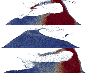
Nevertheless, the accuracy of this approach is largely dependent upon the size and number of mesh cells that are used in a given case. In an ideal scenario, regardless of the scale of the problem, one would use the maximum number and the smallest size of cells possible to capture all the fine-scale fluid features. However, this comes with a considerable computational trade-off. Increasing the number of cells boosts the number of computations that must be carried out for a particular domain. Therefore, depending on the problem, one must find compromises between fast, but inaccurate/accurate, and slow solutions. Sometimes it is possible to decrease the speed of the simulations by conducting mesh independence analysis to determine the largest size of mesh that can be used, without a significant loss of accuracy. But even then, improvements in CPU speeds are usually very insignificant. Furthermore, we always want to have the most accurate response and observe the fine-scale features produced by the fluid and solid whether we deal with small- or large-scale systems. Due to this computational obstacle, however, it has been generally accepted to use fine-mesh systems for small problems. Thus, observing such features for large problems is either not possible, or one must invest significant computational resources to accomplish it, which is often prohibitive. The comparison between coarse- and fine-scale modelling is shown in figure 1. As demonstrated, the coarse-scale modelling cannot show the fine-scale features and often suffices for a general, and crude, representation.

Figure 1. Comparison between (a) coarse-scale and (b) fine-scale modelling for the same time step.
With the recent developments in machine learning (ML) methods and their successful application to classical engineering problems, various advances have been made to accelerate numerical methods (Kachrimanis, Karamyan, & Malamataris Reference Kachrimanis, Karamyan and Malamataris2003; Ariana, Vaferi, & Karimi Reference Ariana, Vaferi and Karimi2015; Benvenuti, Kloss, & Pirker Reference Benvenuti, Kloss and Pirker2016; Chaurasia & Nikkam Reference Chaurasia and Nikkam2017; Liang et al. Reference Liang, Liu, Martin and Sun2018a,Reference Liang, Liu, Martin and Sunb; Figueiredo et al. Reference Figueiredo, Moldovan, Santos, Campos and Costa2019; Brevis, Muga, & van der Zee Reference Brevis, Muga and van der Zee2020; Prieto Reference Prieto2020). This capacity has also been extended to problems related to fluid dynamics and granular flow (Radl & Sundaresan Reference Radl and Sundaresan2014; Kutz Reference Kutz2017; Wan & Sapsis Reference Wan and Sapsis2018; Fukami, Fukagata & Taira Reference Fukami, Fukagata and Taira2019; Li et al. Reference Fukami, Fukagata and Taira2020a; Park & Choi Reference Park and Choi2020; Aghaei Jouybari et al. Reference Aghaei Jouybari, Yuan, Brereton and Murillo2021) where its applications towards the former has been extensively reviewed (Brenner, Eldredge, & Freund Reference Brenner, Eldredge and Freund2019; Brunton, Noack, & Koumoutsakos Reference Brunton, Noack and Koumoutsakos2020; Fukami, Fukagata, & Taira Reference Fukami, Fukagata and Taira2020a). For example, a ML approach was used for the estimation of gravitational solid flows (Garbaa et al. Reference Garbaa, Jackowska-Strumillo, Grudzien and Romanowski2014). In a study conducted by Antony, Zhou & Wang (Reference Antony, Zhou and Wang2006), a mechanistic neural network was applied to predict the micro-macroscopic behaviour of dense granular systems, subjected to quasi-static shearing. In another relevant study by Farizhandi, Zhao & Lau (Reference Farizhandi, Zhao and Lau2016), a ML method was developed towards modelling the change in the distribution of particles in fluidized beds. ML methods have also been applied to predict the permeability of loosely packed granular systems based on experimental and literature data (Mahdi & Holdich Reference Mahdi and Holdich2017). More importantly, ML has been applied in an Euler–Euler fluid–particle coupling problem to improve a filtered two-fluid model by estimating a drag correction for coarse-mesh simulations (Jiang et al. Reference Jiang, Kolehmainen, Gu, Kevrekidis, Ozel and Sundaresan2019). In their study, they were able to correct the inaccuracies that come with using a large-scale mesh when modelling gas–solid fluidized beds. All such developments have motivated us to tackle the complex problem of fluid–particle interactions using ML with the hope of improving such modelling by learning the phenomena that occur in fine-scale simulations and transferring them to coarse-scale models. Hence, as a result of investigating how ML can be applied to the problem of mesh dependence, one could improve the inherent inaccuracies associated with a coarse mesh when using classical coupling methods and retain the superior computational speed associated with large-mesh systems. In this paper, therefore, we do not aim to criticize the existing drag force models but to demonstrate how ML can potentially be used to enhance those models with lower accuracies for large simulation domains.
This paper, therefore, aims to improve the current multi-physics numerical framework for fluid–particle interactions and offer a more efficient alternative, which can make the application of such models more feasible for various problems in mining, chemical, geotechnical and energy resources, as well as to problems like prevention of debris flow and granular failure hazards. To do so, we will use ML due to its ability to work with large data and find complex relationships among them. In addition, the rationale behind using ML is that the drawbacks of the coupling methods, in particular the fluid dynamics, could be mitigated by substituting some of the controlling computations with ML. To be more specific, we hypothesize that the drag force is the controlling factor in particle displacement, therefore we substitute the drag force calculations for large-scale problems with a ML model trained on fine-scale simulations to predict drag forces during run time based on fluid and particle velocities. Similar attempts have also been made to enhance the resolution of turbulent flows using an image-to-image regression, while we aim to improve the computations of fluid–particle interactions in a two-phase and dynamic system by substituting the drag force calculations in coarse-scale simulation via a pre-trained ML model on a fine-scale simulation (Fukami, Fukagata, & Taira Reference Fukami, Fukagata and Taira2020b; Kim et al. Reference Kim, Kim, Won and Lee2021). The final results of the coarse-scale coupling aided by ML have demonstrated significant improvements and greater similarity with the fine-scale (ground truth) modelling, compared with a classical coarse-scale simulation.
The remainder of this paper is organized as follows: in § 2 we discuss the methodology that we follow for conducting the numerical simulations for the fluid and solid, and we also briefly discuss the proposed ML method. In § 3 we outline the model set-up, its geometry and parameters that were used to conduct the simulations. Section 4 focuses on presenting the results obtained from three models, namely fine-scale, coarse-scale and coarse-scale ML-aided models. Finally, § 5 summarizes and concludes the paper.
2. Methodology
In this section, we will discuss the implemented modelling approaches to simulate fluid–solid interactions, the governing equations of which (i.e. CFD-DEM) can be found in many relevant studies (Xu & Yu Reference Xu and Yu1997; Hager et al. Reference Hager, Kloss, Pirker and Goniva2011; Zhao & Shan Reference Zhao and Shan2013a,Reference Zhao and Shanb; Ku, Li & Løvås Reference Ku, Li and Løvås2015). First, we will elaborate on the major equations that are responsible for the particle–particle and particle–wall interactions. Then, we will discuss the methodology that stands behind the fluid component of the simulation. Third, we will provide the key equations that enable fluid–particle coupling and exchange of forces and momenta. Finally, we will discuss how ML is implemented to improve the capabilities of the utilized modelling and what network architecture was found to be most optimal in our simulations.
2.1. Governing equations – particle system
Most problems in fluid–solid modelling are approached by approximating inter-particle interactions, as in these cases such forces can be averaged (Hinch & Serayssol Reference Hinch and Serayssol1986; Yang et al. Reference Yang, Jing, Kwok and Sobral2019) and treated as lubrication forces. However, in situations where particles are expected to undergo large displacements (i.e. granular column collapse), computing inter-particle interactions requires a greater precision (Topin et al. Reference Topin, Monerie, Perales and Radjaï2012). To this end, the DEM is fully capable of accomplishing this and is a promising methodology for our simulations.
DEM is a rapidly developing tool that has largely impacted the particle technology sector (Höhner, Wirtz & Scherer Reference Höhner, Wirtz and Scherer2013; Vidyapati & Subramaniam Reference Vidyapati and Subramaniam2013; Bertuola et al. Reference Bertuola, Volpato, Canu and Santomaso2016; Mandal & Khakhar Reference Mandal and Khakhar2016; Wan et al. Reference Wan, Wang, Yang, Zhang, Wang, Lin and Yang2018; Zhang et al. Reference Zhang, Jia, Zeng, Han and Xiao2018a,Reference Zhang, Zhang, Tang and Cuib). Since its first formulation, there has been a great improvement in DEM in solving many micromechanical problems (Chen & Qiu Reference Chen and Qiu2012) such as soil consolidation (Cui, Chan, & Nouri Reference Cui, Chan and Nouri2017), erosion (Tang, Chan, & Zhu Reference Tang, Chan and Zhu2017), debris flow entrainment (Payne et al. Reference Payne, Quinnan, Potter and Press2008), granular flow mobility (Xu, Hu & Gao Reference Xu, Hu and Gao2016; Ding & Xu Reference Ding and Xu2018) and soil irregular vibration (Zhang et al. Reference Zhang, Zhang, Qiu and Daddow2016; Zhang et al. Reference Zhang, Jia, Zeng, Han and Xiao2018a,Reference Zhang, Zhang, Tang and Cuib).
In classical DEM, contact forces between objects are calculated by allowing a small overlap between the solid bodies (usually not larger than 5 % of the particle radius), where the forces are proportional to the amount of overlap. Thus, the choice of contact model becomes significant. In this study, since we are interested only in observing mechanical inter-particle behaviour, we adopt the Hertzian force model as it neglects cohesive forces between the particles (Hertz Reference Hertz1882). In our coupled system, the governing equations of particle motion are the classical DEM equations, extended by a force term  $\boldsymbol{F}_i^f$, which accounts for the fluid–particle interactions
 \begin{gather}{m_p}\frac{{\textrm{d}{\boldsymbol{v}_p}}}{{\textrm{d}t}} = \mathop \sum \limits_{{N_{p,w}}} {\boldsymbol{F}_{p,w}} + \boldsymbol{F}_p^f + {m_p}\boldsymbol{g},\end{gather}
 \begin{gather}{I_p}\frac{{\textrm{d}{\boldsymbol{\omega }_p}}}{{\textrm{d}t}} = \mathop \sum \limits_{{N_{p,w}}} {\boldsymbol{M}_{p,w}},\end{gather}
where m p is particle mass,  ${\boldsymbol{v}_p}$ is the velocity of particles,
  ${\boldsymbol{F}_{p,w}}$ particle–particle or particle–wall force,
  $\boldsymbol{F}_p^f$ is the particle–fluid interaction force,
  $\boldsymbol{g}$ is gravitational acceleration,
  ${\boldsymbol{\omega }_p}$ is the angular velocity,
  ${I_p}$ is the moment of inertia and
  ${\boldsymbol{M}_{p,w}}$ is the moment acting on particles, created either by other particles or walls. The particle–fluid interaction term
  $\boldsymbol{F}_p^f$ accounts for all fluid–solid interaction forces, namely the pressure gradient force
  ${\boldsymbol{F}_{\boldsymbol{\nabla }p}}$, drag force
  ${\boldsymbol{F}_d}$, viscous force
  ${\boldsymbol{F}_{\boldsymbol{\nabla }\boldsymbol{\cdot }\tau }}$, virtual mass force
  ${\boldsymbol{F}_{vm}}$, Basset force
  ${\boldsymbol{F}_B}$, Saffman force
  ${\boldsymbol{F}_{Saff}}$ and Magnus force
  ${\boldsymbol{F}_{Mag}}$ (Crowe et al. Reference Crowe, Schwarzkopf, Sommerfeld and Tsuji2011)
 \begin{equation}\boldsymbol{F}_p^f = {\boldsymbol{F}_{\boldsymbol{\nabla }p}} + {\boldsymbol{F}_d} + {\boldsymbol{F}_{\boldsymbol{\nabla }\boldsymbol{\cdot }\tau }} + {\boldsymbol{F}_{vm}} + {\boldsymbol{F}_B} + {\boldsymbol{F}_{Saff}} + {\boldsymbol{F}_{Mag}}.\end{equation}
In most scenarios, the first three forces account for the majority of fluid–particle forces, and others may be neglected. Therefore, in our models we use
 \begin{equation}\boldsymbol{F}_p^f = {\boldsymbol{F}_{\boldsymbol{\nabla }p}} + {\boldsymbol{F}_d} + {\boldsymbol{F}_{\boldsymbol{\nabla }\boldsymbol{\cdot }\tau }}.\end{equation}
 As mentioned earlier, the Hertzian contact force model along with Coulomb's friction law are responsible for describing the interactions between particles (i.e.  ${\boldsymbol{F}_{p,w}}$).
We use the Koch–Hill drag force (Koch & Hill Reference Koch and Hill2001), given by
 \begin{equation}{\boldsymbol{F}_d} = \frac{{{V_p}\beta }}{{{\gamma _p}}}({\boldsymbol{u}_f} - {\boldsymbol{v}_p}),\end{equation}
where  ${V_p}$ denotes particle volume and
  $\beta $ is the interphase momentum exchange term, defined by
 \begin{equation}\beta = \frac{{18{\mu _f}\gamma _f^2{\gamma _p}}}{{d_p^2}}\left( {{F_0}({\gamma_p}) + \frac{1}{2}{F_3}({\gamma_p})R{e_p}} \right),\end{equation}
where  ${\gamma _f}$ is local porosity (volume fraction of fluid in a given cell),
  ${\gamma _p}$ is the volume fraction of solid
  $({\gamma _f} + {\gamma _p} = 1)$ and
 \begin{equation}R{e_p} = \frac{{{\gamma _f}{\rho _f}|{\boldsymbol{u}_f} - {\boldsymbol{v}_p}|{d_p}}}{{{\mu _f}}},\end{equation}
where  ${\rho _f}$ is the fluid density,
  ${\boldsymbol{u}_f}$ and
  ${\boldsymbol{v}_p}$ are fluid and particle velocities, respectively,
  ${d_p}$ is particle diameter and
  ${\mu _f}$ is fluid viscosity.
Furthermore, functions  ${F_0}$ and
  ${F_3}$ are given as
 \begin{gather}{F_0}({\gamma _p}) = \left\{ {\begin{array}{@{}ll} {\dfrac{{1 + 3\sqrt {\dfrac{{{\gamma_p}}}{2}} + \dfrac{{135}}{2}{\gamma_p}\ln ({\gamma_p}) + 16.14{\gamma_p}}}{{1 + 0.681{\gamma_p} - 8.48\gamma_p^2 + 8.16\gamma_p^3}}}&{\textrm{if}\;{\gamma_p} < 0.4}\\ {\dfrac{{10{\gamma_p}}}{{\gamma_f^3}}}&{\textrm{if}\;{\gamma_p} \ge 0.4} \end{array}} \right.,\end{gather}
 \begin{gather}{F_3}({\gamma _p}) = 0.0673 + 0.212{\gamma _p} + \frac{{0.0232}}{{\gamma _f^5}}.\end{gather}
2.2. Governing equations – fluid system
Computational fluid dynamics (CFD) uses numerical analysis and data structures to analyse and solve problems that involve fluid flows and has been applied to a wide range of research and engineering problems. In this paper, CFD is coupled with DEM to calculate the drag, pressure gradient and viscous forces. To do so, the fluid domain is discretized into a set of cells, and the following governing equations are solved at each cell for locally averaged state variables, such as pressure, density and fluid velocity:
 \begin{gather}\frac{\partial }{{\partial t}}({\gamma _f}{\rho _f}\; ) + \boldsymbol{\nabla }\boldsymbol{\cdot }({\gamma _f}{\rho _f}) = 0,\end{gather}
 \begin{gather}\frac{\partial }{{\partial t}}({\gamma _f}{\rho _f}{\boldsymbol{u}_f}) + \boldsymbol{\nabla }\boldsymbol{\cdot }({\gamma _f}{\rho _f}{\boldsymbol{u}_f}{\boldsymbol{u}_f}) ={-} {\gamma _f}\boldsymbol{\nabla }p - {K_{pf}}({\gamma _f}{\tau _f}) + \boldsymbol{\nabla }\boldsymbol{\cdot }({\gamma _f}{\tau _f}) + {\gamma _f}{\rho _f}\boldsymbol{g} + \boldsymbol{f},\end{gather}
where  ${\gamma _f}$ is the void fraction (fluid content of a calculation cell),
  ${\rho _f}$ is the fluid density,
  ${\boldsymbol{u}_f}$ is the fluid velocity, p is pressure,
  ${\tau _f}$ is the liquid stress tensor,
  $\boldsymbol{g}$ is the gravity vector and
  ${K_{pf}}$ is the implicit particle–fluid momentum exchange term given by
 \begin{equation}{K_{pf}} = \frac{{{\gamma _f}.\left|{\sum\limits_p {{\boldsymbol{F}_d}} } \right|}}{{{V_{cell}}.|{\boldsymbol{u}_f} - {\boldsymbol{v}_p}|}}.\end{equation}
In this approach, interaction forces for each particle are calculated first. To obtain  ${K_{pf}}$, the forces of all particles in each fluid cell are summed.
2.3. ML Assisted Modelling
The model uses five variables as inputs, namely: (i) particle velocity in the X direction  $({\boldsymbol{v}_{p,x}})$, (ii) particle velocity in the Z direction
  $({\boldsymbol{v}_{p,z}})$, (iii) fluid velocity in the X direction
  $({\boldsymbol{u}_{f,x}})$, (iv) fluid velocity in the Z direction
  $({\boldsymbol{u}_{f,z}})$, (v) void fraction. These variables are connected to two outputs which are the drag forces in the X and Z directions
  $({\boldsymbol{F}_{d,x}},\; {\boldsymbol{F}_{d,z}})$. The training set is obtained from the fine-scale modelling with a cell size of 4 cm, particle size of 0.1 cm and where the number of particles = 41 500; see figure 2. The fluid and particle properties of the training are identical to the ground truth modelling, as well as simulation control parameters such as time step and coupling interval. The training case was simulated for 7.5 s of free fall of the particle column. The architecture of the utilized ML is provided in figure 4. In particular, a multilayer-perceptron neural network model was used for this task. In this paper, we optimized the architecture of the utilized network using the grid search method, which is a common method for parameter tuning (Liashchynskyi & Liashchynskyi Reference Liashchynskyi and Liashchynskyi2019). This method automatically adjusts the hyperparameters by searching all possibilities and combinations such that the final estimations are optimum. Then, the final ML model is derived and used for all computations. An example of the effect of the number of layers and their neurons is provided in figure 3. In this study, a network with three hidden layers and [170 70 30] neurons is used, which resulted in a model with an average accuracy coefficient of
  ${R^2} = 0.8408$. Based on the further sensitivity analysis (table 1), we found that the exponential linear unit (ELU) activation function, mean squared error (MSE) loss function and training set that consists of 250 000 data points resulted in higher prediction accuracies. Model training specifications are summarized in table 2. In this paper, all
  ${R^2}$ values signify the average
  ${R^2}$ of
  ${\boldsymbol{F}_{d,x}}$ and
  ${\boldsymbol{F}_{d,z}}$, which is calculated using
 \begin{equation}{R^2}_{(y,\hat{y})} = 1 - \frac{{\sum\limits_{i = 1}^n {{{({y_i} - {{\hat{y}}_i})}^2}} }}{{\sum\limits_{i = 1}^n {{{({y_i} - \bar{y})}^2}} }},\end{equation}
where  ${y_i}$ is the true value of ith sample–
  ${\hat{y}_i}$ represents the predicted value for total n samples, and
  $\bar{y} = (1/n)\sum\nolimits_{i = 1}^n {{y_i}} $, i.e. the mean of the observed data.

Figure 2. Numerical model set-up and the initial position of granular particles of the training dataset.

Figure 3. Sensitivity analysis of the effect of the number of layers and neurons on prediction accuracy, using the ELU activation function. The numbers in the matrix indicate  ${R^2}$.

Figure 4. Our proposed ML architecture for estimating the drag force in the X and Z directions.
Table 1. Summary of sensitivity analysis for different parameters in our proposed ML network.

Table 2. Specifications used for training.

In this study, we assign an activation function to each node (neuron) of the network and determine whether the neuron should be activated, which depends on whether the input of that neuron is relevant to the prediction or not. To be more specific, we used the ELU activation function for all hidden layers. The output of this function is determined based on the following equation:
 \begin{equation}y = \left\{ {\begin{array}{@{}ll} {\alpha ({e^x} - 1)}&{\textrm{if}\;x \le 0}\\ x&{\textrm{if}\;x > 0} \end{array},} \right.\end{equation}
where  $\alpha $ is a coefficient. In most cases, this parameter is chosen to be between 0.1 and 0.3. The outputs of this activation function, therefore, range from slightly below zero (exponential relation in the case of
  $x < 0$) and
  $y = x$ (linear relation in the case of
  $x > 0$). To compare the effect of the activation function on the a posteriori results of the simulation we chose the three activation functions that performed best during the sensitivity analysis phase, namely ELU, Rectified Linear Unit (ReLU, table 1) and smooth approximation of ReLU (Softplus, table 1), and conducted three ML-assisted simulations on an 8 cm mesh. The results are shown in figure 5. Based on the visual analysis of the results, we concluded that ELU is optimal in terms of prediction accuracy during a priori training, and when used for a posteriori coarse-scale ML-assisted simulation. These results are also shown quantitatively in figure 6.

Figure 5. Runoff, velocity and drag force evolution for ground truth fine-scale (4 cm mesh) CFD-DEM, coarse-scale (8 cm mesh) ML-assisted modelling using the ELU activation function, coarse-scale (8 cm mesh) ML-assisted modelling using the ReLU activation function and coarse-scale (8 cm mesh) ML-assisted modelling using the Softplus activation function.

Figure 6. Quantitative comparison between the performances of several activation functions on the prediction capability of the proposed ML model.
Another indispensable part of any neural network is a loss (cost) function. This function calculates the difference between the output of the algorithm and the true values, and it evaluates how well the model predicts the target values. The goal of the network is to minimize the output of the loss function and thereby increase the accuracy of predictions. For our network, we used the MSE loss function, which follows the expression below
 \begin{equation}\textrm{MSE} = \frac{{\sum\limits_{i = 1}^n {{{({y_i} - y_i^p)}^2}} }}{n},\end{equation}
where  ${y_i}$ and
  $y_i^p$ are true and predicted values, respectively, and n is the number of samples/data.
To find the optimal weights and eventually minimize the loss function, we used backpropagation, which is a widely used algorithm in the training of ML. In this concept, the gradients of the activation functions in each successive neuron are tracked to optimize the weights and reduce the loss function. The gradients are then used by an optimization algorithm – AdaMax in our case – to update the model weights (Kingma & Ba Reference Kingma and Ba2015). It ultimately calculates to what degree the output values are affected by each individual weight of the model, by going back from the error function to a specific weight of a neuron.
The dataset was randomly split as follows: 85 % (212 500 data points) for training and 15 % (37 500 data points) for validation and 20 000 data points were used for testing. It should also be noted that only 2.3 % of the fine-scale data, which are generated from the training model (figure 2), are used for training. The reason for this was to make sure that the trained network is not biased toward the training and boundary conditions.
3. Model set-up
To demonstrate the performance of our proposed method, we used a two-dimensional polygonal pack with 20 000 spherical particles and water as an ambient fluid, where the properties of both phases are listed in table 3. For the coupling parameters between fluid and solid, we used a coupling interval of 50 (meaning that one CFD step is coupled with DEM after 50 DEM steps), and the drag force model was chosen to be the Koch—Hill model, as using this model we observed the greatest discrepancy between the fine and coarse cases. A schematic representation of the considered physical domain is shown in figure 7. As can be seen, this model is very different from the one we used for training the ML model (figure 2).

Figure 7. Numerical model set-up and the initial position of the utilized granular system for testing the proposed ML model.
Table 3. Model parameters used in the granular failure simulation.

The simulations were carried out in parallel using 4 cores of an Intel i7-7700 CPU. The computational times of the simulations for fine (4 cm), coarse (8, 16, 32 cm) and coarse (8, 16, 32 cm) ML-assisted cases are presented in table 3. The trained network was converted to C++ and executed during run time to produce the desired drag force using the particle velocity, fluid velocity and void fraction as inputs. Figure 8 demonstrates the accuracy of the predictions using the ML-assisted model, where true values are the drag forces obtained from fine-scale modelling, (a) shows the model performance using identical input parameters as the fine-mesh simulation and (b–d) represent model performance using the averaged input values of the fluid velocity and void fraction according to the respective mesh resolution. Generally, the model demonstrates good predictions for the entire data range. It can be noted, however, that the accuracy of the predictions diminishes when the data approach negative values. This observation can be explained by the fact that the data in the training set are mostly positive, and the model did not have sufficient data (compared with the positive values) to be as accurate for negative values.

Figure 8. Parity plots between predicted and exact values of  ${\boldsymbol{F}_{d,x}}$ and
  ${\boldsymbol{F}_{d,z}}$; (a) fine scale (4 cm mesh), (b) coarse scale (8 cm mesh), (c) coarse scale (16 cm mesh), and (d) coarse scale (32 cm mesh).
4. Results and discussion
In this study, seven simulations were performed on the geometry shown in figure 7, using the particle and fluid properties listed in table 3. To observe the differences between the fine and coarse models and then to be able to improve the coarse simulation, we conducted an injection simulation in a granular pack, where the first case, representing fine-scale modelling, was performed using a 4 cm mesh and the second, third and fourth cases, representing the coarse-scale modelling, were performed using 8, 16 and 32 cm meshes, respectively. Similarly, the force computations were replaced with a ML model for the final drag force predictions in the later coarse models. The drag predictions (in the X and Z directions) are based on five inputs (particle and fluid velocities in the X and Z directions, and void fraction)
First, we visually discern substantial differences between the fine and coarse simulations in terms of particle runoff evolution and the final height of the granular system; see figure 9. Clearly, using a coarse mesh to solve the fluid–particle interactions results in a considerable loss in the ability of the utilized numerical simulation to demonstrate fine-scale features, and the coupling of the drag force between the fluid and solid becomes less accurate. This can be observed at all stages of the simulation and is most apparent during the first 1.5 s of injection, where the shock wave-like propagation of the granular system is observed in fine-scale modelling but is not present in the coarse modelling. We observe that, towards the first 40 % of the simulation time, the granular system in the coarse case has almost attained a form that is close to its final shape, without any considerable variation in height or increase in runoff, while the shape of the granular system in the fine mesh is very dynamic and the outer boundary of the granular system is gradually moving towards the outlet throughout the simulation. Furthermore, due to using a coarse mesh, the effect of the drag force on the particles becomes insignificant to the degree that water flow is reserved to a corner flow at the top of the domain, without affecting the particles underneath. This fact poses a problem, since, if a similar case was only performed on a coarse mesh and if it was related to a natural system, such as landslides or avalanches, then this modelling would present an overly optimistic result. The difference between the fine and coarse modelling in terms of the effects of the drag force can be visually confirmed in figures 9(a) and 9(b). As can be seen, the influence of the drag force on the movement of particles is much more significant in the case of fine-mesh modelling than it is in the coarse-mesh simulation. Therefore, it is clear at this point that the discrepancies between the fine and coarse models are substantial.

Figure 9. Runoff and drag force evolution for (a) ground truth fine-scale (4 cm mesh) CFD-DEM, (b) three coarse-scale CFD-DEM (8, 16, 32 cm meshes) and (c) coarse-scale (8, 16, 32 cm mesh) ML-assisted modelling.
In figure 9(c), we present the results for ML-assisted modelling using a coarse mesh. From a visual examination of the evolution of the particle positions, we observe that the results of the proposed method using 8 and 16 cm mesh sizes are far closer to the fine-scale modelling, i.e. figure 9(a), than the corresponding coarse modelling, i.e. figure 9(b), even though we are still using a coarse mesh to conduct this simulation. We note that, at all stages of the simulation, the proposed ML-assisted modelling using the two mesh sizes mentioned above is much more similar to the fine case, indicating that the inherent issue of the loss in the accuracy associated with using a coarse mesh has been greatly improved. A simple visual comparison shows that the shape of the granular system at all stages of the simulation resembles the fine case. Furthermore, we observe that the height and run-off distance, in all ML-assisted cases, are dynamic, in contrast to the original coarse cases. Moreover, the distribution of the drag forces which are shown in figure 9 demonstrates that, although coarse mesh is used, the coupling between the fluid flow and particles is far superior in the ML-assisted case than in regular coarse-scale modelling. Figure 10 further demonstrates the ability of the proposed ML-assisted modelling to compensate for inaccuracies when using a coarse mesh. Here, one can observe that, proportionally to the drag force distribution, velocities of individual particles in the case of fine-scale modelling and the proposed ML-assisted simulation (more so in the 8 and 16 cm cases) are largely similar and reside on the same scale at all stages of injection. Whereas the original coarse modelling demonstrates a comparative lack of particle movement.

Figure 10. Runoff and particle velocity evolution for (a) ground truth fine-scale (4 cm mesh) CFD-DEM, (b) three coarse-scale CFD-DEM (8, 16, 32 cm meshes) and (c) coarse-scale (8, 16, 32 cm meshes) ML-assisted modelling.
The differences in the velocities in the system can be further observed in the evolution of the fluid velocity presented in figure 11. Here, we note that, as opposed to the fine mesh and ML-assisted modelling, the coarse-mesh modelling demonstrates a comparative lack of turbulent flow and vorticity in the system. The flow in the coarse-mesh modelling becomes relatively stable at the early stages of the simulation and the presence of the solid exerts only a superficial influence on the flow, compared with the original fine-scale case and the corresponding ML-assisted coarse cases. We also observe that, towards the fifth second of the simulation, the distribution of fluid velocities in the case of coarse-mesh modelling demonstrates a trend towards a sharp transition from smaller to larger velocities. This trend is also confirmed quantitatively in figure 15.

Figure 11. Fluid velocity evolution for (a) ground truth fine-scale (4 cm mesh) CFD-DEM, (b) three coarse-scale CFD-DEM (8, 16, 32 cm meshes) and (c) coarse-scale (8, 16, 32 cm meshes) ML-assisted modelling.
In order to quantitatively compare the results for all three cases, we plotted several important and quantifiable parameters, which will assist us in conducting a more rigorous and detailed comparison. To be able to have a general understanding of the distribution of data in the domain, the average behaviours are compared. Furthermore, in some cases, and if necessary, more information is also provided. First, as the most important parameter in our methodology, the drag force data are presented in figure 12(a). The results suggest that the drag force data in the first two ML-assisted modelling cases (using 8 and 16 cm mesh sizes) are significantly closer to the ground truth case (fine-mesh modelling) than the corresponding coarse-mesh cases, and the last ML-assisted case (32 cm mesh) can also be considered an improvement as compared with the corresponding CFD-DEM case, but to a lesser degree. The proposed ML-assisted cases reflect the major spike in drag forces that are observed around first second of the simulation. Additionally, in order to confirm that the results of the simulations can be reliably reproduced by conducting identical a priori ML training and using the produced network for future simulations, we conducted three identical trainings (each time with a different seed number) which are then used on the same coarse-scale ML-assisted simulations (8 cm mesh). This analysis allows one to observe how ML models with different initializations can affect the responses. These results are presented in figure 12. Here, the upper and lower bounds of the cloud region indicate the maximum and minimum values obtained from coarse-scale ML-assisted simulation for a particular time step.

Figure 12. Comparison of average drag force evolution using fine (4 cm) mesh CFD-DEM; coarse (8 cm) mesh CFD-DEM using three most common models for calculating drag force, i.e. Koch–Hill, Di Felice, Gidaspow; and ML-assisted coarse (8 cm) CFD-DEM modelling.
Furthermore, to see how our ML-assisted modelling performs compared with other well-established methodologies for calculating the drag force, we selected two additional methods, namely those of Di Felice (Reference Di Felice1994) and Gidaspow (Reference Gidaspow1994), and performed identical CFD-DEM flow simulations using an 8 cm mesh. A quantitative comparison of the average drag force evolution is provided in figure 12. The individual drag force evolution curves suggest that the two additional classical drag force models perform very similarly to the Koch–Hill model, and demonstrate similarly poor performance on the coarse grid, compared with the ML-assisted modelling.
Another observation that we consider is that the spike in the case of the proposed ML-assisted modelling (for all mesh sizes, but less noticeably for 32 cm) comes 0.1–0.2 s earlier than in the ground truth case. This can also be confirmed by visual examination of the shape evolution snapshots in figures 9 and 10, where the top of the granular wave at the upper part of the domain in the case of ML-assisted modelling is moving ahead of the one shown in the ground truth case. Next, the particle velocities are shown in figure 13(b). Here, the similarity of the ML-assisted modelling to the fine-scale ground truth is even more apparent. More importantly, even at the 16 cm mesh size, where a significant discrepancy between the fine and coarse scales is expected, the ML-assisted modelling results are substantially closer to the ground truth than the corresponding coarse CFD-DEM, and the 32 cm ML-assisted case demonstrates a spike on a similar scale, however, its overall shape is less comparable to the original fine-scale CFD-DEM modelling. The third set of comparisons includes particle–particle and particle–wall collision forces; see figure 13(c). Here, the largest spikes (around 1 s) correspond to the moment when the particles hit the upper wall of the domain. The average values of the forces around 1 s quantitatively demonstrate that the collision forces in the cases of coarse-scale modelling are very insignificant, compared with the ground truth and the ML-assisted (8 and 16 cm) modelling, which is also evident visually in the snapshots shown in figures 9 and 10. The ML-assisted (32 cm) case, however, demonstrates no improvement in terms of collision force evolution. Next, the evolution of kinetic energy in the pack is shown in figure 13(d).

Figure 13. Uncertainty quantification of the effect of different initializations on the proposed ML model for predicting (a) drag force, (b) particle velocity, (c) collision force and (d) kinetic energy evolution of the granular system. The pink colour indicates fluctuations of the ML-assisted modelling (8 cm), where the solid red curve indicates the average value based on the conducted simulations.
One of the most important quantifiable physical properties that we present in this study is the comparison of runoff and height evolution between all three cases; see figure 14. Here, we can confirm the previous visual observations regarding the differences between the fine- and coarse-scale modelling, and the similarities of fine-scale and ML-assisted simulations. The final run-off distance at the fifth second of the simulation for the ground truth CFD-DEM case (4 cm mesh) was 9.1 m, 5.9, 6.5, 6.9 m for the coarse-scale (8, 16, 32 mesh sizes) CFD-DEM and 9.5, 8.5, 9.4 m for the ML-assisted (8, 16, 32 mesh sizes) cases, respectively. In terms of the final height of the granular system, the values are 0.856 m (ground truth), 1.353, 1.151, 0.903 m (8, 16, 32 mesh sizes CFD-DEM) and 0.876, 0.94, 0.7 m (8, 16, 32 mesh sizes ML assisted). We also confirm that the height and run-off distance of the coarse-scale case undergo almost no changes after the first 2 s of the simulation, which is observed visually in figures 9 and 10 (except for height evolution of 8 cm mesh CFD-DEM modelling).

Figure 14. Runoff (a) and height (b) evolution of the granular system for fine-scale, coarse-scale and ML-assisted cases.

Figure 15. Evolution of average pressure of the fluid phase for fine-scale, coarse-scale and ML-assisted cases.
Another metric that we have included in this paper is the fluid pressure evolution; see figure 15. Compared with the coarse-scale simulation, the pressure values of the ML-assisted modelling are much closer to the fine-scale modelling, than in the original coarse-scale case. All ML-assisted cases are characterized by a major spike, similar to the ones found in other evolution plots (e.g. drag force, particle velocity, etc.). As expected, the overall resemblance to the fine scale diminishes with the increase in mesh size, where using 32 cm mesh resulted in a considerably less similar curve shape.
We also have compared the fluid velocity for all cases and the results are shown in figure 16. Here, the average values in all three cases are relatively similar. However, the median values suggest that the transition between the values of fluid velocity is much sharper in the case of coarse-scale CFD-DEM (8 cm mesh size) modelling. All these visual and quantitative comparisons between the three cases suggest that the shortcoming of coarse-scale modelling has for the most part been largely improved by combining it with a ML model previously trained on ground truth fine-scale data.

Figure 16. Evolution of velocity of the fluid phase for fine-scale, coarse-scale and ML-assisted cases; (a) average, (b) median.
5. Conclusions
The importance of studying fluid–solid interactions is manifested in a large number of areas of science and engineering. It is, therefore, very important to have fast and accurate models that allow the modelling of these phenomena. Several computational techniques are used for simulating fluid–particle interactions, among which the coupling of CFD and DEM has proven to be most convenient in terms of computational costs, accuracies of predictions and complexity of implementation. However, the most prominent limitation of this approach is that it is largely dependent on the size of the mesh of the fluid domain.
The fact is, when the coupling is conducted on a large-scale mesh, even though it results in faster simulations, the results are inaccurate, and the fine-scale features are not reproduced. On the other hand, when such modelling is used with a small-scale mesh, even though it results in significantly more accurate results, the computational time becomes prohibitive. One widely used approach to increase the size of the mesh while still retaining the accuracy of the modelling is to conduct a mesh-independence analysis, where scientists and engineers determine how much they can increase the size of the mesh and still obtain results that are still acceptably accurate. This method, however, usually results only in minor improvements in computational speeds. Therefore, it is still a challenge in the scientific community to find a way to be able to have both accurate and fast modelling using larger meshes.
In this paper, we proposed a coupled and assisted ML approach, where one of the major forces responsible for fluid–solid coupling is replaced with a ML model, which was previously trained on a ground truth fine-scale simulation. This framework ultimately allows more accurate modelling, while still using a coarse mesh. To test the capabilities of the new method, we conducted seven simulations, where the first case was fine-scale modelling (ground truth), the second, third and fourth were coarse-scale simulations (considerably less accurate, with mesh sizes of 8, 16 and 32 cm, respectively) and the final three cases were coarse-scale ML-assisted modelling on the same mesh sizes. The results of this research have demonstrated large improvements in 9 metrics, the most significant of which are run-off distance and height of the granular system, fine-scale features and the computation speedup. However, it should be noted that the effectiveness of this method was considerably diminished when used with a 32 cm mesh. One possible avenue for future research might be to reduce the computational cost using pruning operations of the ML model (Fukami et al. Reference Fukami, Hasegawa, Nakamura, Morimoto and Fukagata2021; Mitra et al. Reference Mitra, Venkatesan, Jangid, Nambiar, Kumar, Roa, Santo, Haghshenas, Mitra and Schmidt2021).
Acknowledgements
We would like to thank the anonymous reviewers who provided constructive comments on the earlier draft of the manuscript.
Funding
This study was partially supported by NSF (Grant no. CMMI-2000966) (Fluid Dynamics), NIH (Grant no. P20GM103432) and NASA (Grant no. 80NSSC19M0061).
Declaration of interests
The authors report no conflict of interest.


