2.1. Linear models

For small-amplitude waves, the system given by (2.1) can be linearized to

(2.2a,b)\begin{equation} \zeta_t=W, \quad {\varPhi}_t + g\zeta = 0.\end{equation}

In the meantime, $\varPhi$ and $W$ can be approximated by those evaluated at the mean free surface ($z=0$) so that $\varPhi \simeq \phi (\boldsymbol x,0,t) = \phi _0(\boldsymbol x,t)$ and $W\simeq \phi _z(\boldsymbol x,0,t)=w_0(\boldsymbol x,t)$.

When the three-dimensional Laplace equation is solved for $\phi$ imposing the bottom boundary condition given by $\partial \phi /\partial z\vert _{z=-h} = 0$, its solution can be written, in Fourier space, as

(2.3)\begin{equation} \hat \phi(\boldsymbol k,z,t)= \{\cosh [k(z+h)]/\cosh(kh) \} \hat \phi_0 (\boldsymbol k,t), \end{equation}

where $\hat f (\boldsymbol k,z,t)$ is the Fourier transform of $f(\boldsymbol x,z,t), k=\vert \boldsymbol k\vert$ with $\boldsymbol k$ being the two-dimensional wavenumber vector and $h$ is the constant water depth. Then, from (2.3), one can obtain

(2.4)\begin{equation} \hat w_0(\boldsymbol k,t)=(k\tanh kh) \hat \phi_0(\boldsymbol k,t), \end{equation}

from which the approximate expression for $W$ is given, in terms of $\varPhi$, by

(2.5)\begin{equation} \hat W(\boldsymbol k,t)\simeq (k\tanh kh) \hat \varPhi(\boldsymbol k,t).\end{equation}

Finally, after taking the Fourier transform of (2.2) and using (2.5), the linear evolution equations for $\zeta$ and $\varPhi$ can be written, in Fourier space, as

(2.6a,b)\begin{equation} \hat \zeta_t=(k\tanh kh) \hat \varPhi, \quad {\hat \varPhi}_t + g\hat \zeta = 0.\end{equation}

For $(\hat \zeta, \hat \varPhi ) \sim \exp (-{\rm i}\omega t)$, (2.6) yields the full linear dispersion relation for surface gravity waves given by

(2.7)\begin{equation} \omega^2=gk\tanh kh,\end{equation}

from which one can see that the wave frequency $\omega$ is always real as $k>0$.

For long waves ($kh\ll 1$), ${\mathcal {T}}=\tanh kh$ can be expanded as

(2.8)\begin{equation} {\mathcal{T}}= \sum_{n=0}^\infty \frac{2^{2n+2}(2^{2n+2}-1)B_{2n+2}}{(2n+2)!}(kh)^{2n+1},\end{equation}

where $B_{2n}$ are the Bernoulli numbers given by $B_0=1, B_2=1/6, B_4=-1/30, B_6=1/42, \ldots$. This infinite series converges to $\tanh kh$ as long as $kh<{\rm \pi} /2$ (due to singularities at $kh=\pm {\rm i} ({\rm \pi} /2)$ in the complex $k$-plane), but, when it is approximated for long waves, its behaviour depends sensitively on how it is truncated.

When the upper limit for the summation in (2.8) is replaced by an integer $M (\ge 0)$, the truncated linear system (2.6) is given by

(2.9a,b)\begin{equation} \hat \zeta_t=k{\mathcal{T}}_M \ \hat \varPhi, \quad {\hat \varPhi}_t + g\hat \zeta = 0,\end{equation}

where ${\mathcal {T}}_M$ represents the $M$th-order long wave approximation of ${\mathcal {T}}$ valid to $O(\beta ^{2M})$ as $kh=O(\beta )$. The linear dispersion relation of this truncated system is then given by

(2.10)\begin{equation} \omega^2 \simeq ghk^2\left[1-\frac{1}{3}(kh)^2+\frac{2}{15} (kh)^4 +\cdots+ \frac{2^{2M+2}(2^{2M+2}-1)B_{2M+2}}{(2M+2)!}(kh)^{2M}\right].\end{equation}

Now one can see that, if $M$ is an odd integer, the right-hand side of (2.10) becomes negative for large $k$ so that $\omega$ becomes purely imaginary. As the imaginary part of $\omega$, or the growth rate is proportional to $k^{M+1}$, it increases without bound as $k\to \infty$ and, therefore, the truncated system with odd $M$ is ill-posed. For example, as shown in figure 1(a), short-wavelength disturbances of $kh\gtrsim 1.732$ and $kh\gtrsim 1.647$ are unstable with the growth rates proportional to $k^2$ and $k^4$ for $M=1$ and 3, respectively. Under the linear assumption, as the free surface velocity potential $\varPhi$ can be approximated by the mean level velocity potential $\phi _0$, this discussion is parallel to that for the long wave model for $\phi _0$ in Madsen & Schäffer (Reference Madsen and Schäffer1998).

Figure 1. Linear dispersion relations between the wave frequency $\omega$ and the wavenumber $k$ for the systems for (a) the surface potential; (b) the depth-averaged velocity; (c) the bottom potential given by (2.10), (2.13) and (2.16), respectively. Three different approximations (dotted: $M=1$; dashed: $M=2$; dash-dotted: $M=3$) are compared with the full dispersion relation of the linearized Euler equations (solid) given by (2.7). The vertical line in (b) shows the value of $k_c$, where a singularity appears for $M=2$.

If $M$ is an even integer, the wave frequency $\omega$ is always real, but $\omega \sim k^{M+1}$ increases rapidly with $k$. This requires one to use a very small time step when the system for $\zeta$ and $\varPhi$ is solved numerically as the criterion for numerical stability for a time integration scheme can be written as $\omega \Delta t\le C$, with $C$ being a constant depending on the scheme. Therefore, the long wave model for the surface variables ($\zeta$ and $\varPhi$) with any $M$ might be inappropriate for numerical computations.

Instead of the surface velocity potential $\varPhi$, the well-known Boussinesq equations are often written in terms of the depth-averaged velocity defined by

(2.11)\begin{equation} {\bar{\boldsymbol u}}=\frac{1}{(h+\zeta)}\int_{{-}h}^{\zeta} \boldsymbol{\nabla} \phi\, {\rm d} z.\end{equation}

For small-amplitude waves, after replacing the upper limit of the integration by $0$ and using (2.3), the Fourier transform of $\bar {\boldsymbol u}$ can be approximated by $\hat {\bar {\boldsymbol u}} \simeq -{\rm i} \boldsymbol k \{\tanh kh/(kh)\} \hat \varPhi$, from which we have $h \widehat {\boldsymbol {\nabla } {{\boldsymbol \cdot }} \bar {\boldsymbol u}} \simeq -(k\tanh kh) \hat {\varPhi }$. Then, from (2.9), the linear system for $\zeta$ and $\bar {\boldsymbol u}$ can be found, in Fourier space, as

(2.12a,b)\begin{equation} \hat \zeta_t ={-} h \widehat{\boldsymbol{\nabla} {{\boldsymbol \cdot}} \bar{\boldsymbol u}}, \quad (kh\coth kh) \hat{\bar{\boldsymbol u}}_t +g \widehat{\boldsymbol{\nabla} \zeta}=0. \end{equation}

For a long wave, when truncated at $O(\beta ^{2M})$, the linear system (2.12) yields the following dispersion relation

(2.13)\begin{equation} \left[1+\frac{1}{3}(kh)^2-\frac{1}{45}(kh)^4+\cdots +\frac{2^{2M}B_{2M}}{(2M)!} (kh)^{2M}\right] \omega^2 \simeq ghk^2, \end{equation}

where the expansion on the left-hand side of (2.13) is the truncated Taylor series of $kh\coth kh$. Contrary to the system for the surface velocity potential $\varPhi$, the system for the depth-averaged velocity is well-posed for odd $M$, but is problematic for even $M$. For example, for $M=2$, the system is unstable for disturbances of $k>k_c$ with $k_ch=[(15+9\sqrt {5})/2]^{1/2}\simeq 4.191$. Although the growth rate decreases to 0 as $k\to \infty$, there is a singularity at $k=k_c$, where the growth rate becomes infinity, as shown in figure 1(b). This implies that the depth-averaged system given by (2.12) with even $M$ should avoided (Matsuno Reference Matsuno2016). On the other hand, for odd $M$, the wave frequency $\omega$ is real and approaches zero as $k$ increases, which is ideal for numerical stability, as discussed previously. Therefore, the depth-averaged system only with odd $M$ would be useful for numerical computations.

Another variable often adopted for long wave models is the bottom velocity potential, or the bottom velocity. For small-amplitude waves, $\varPhi$ and the bottom velocity potential $\phi _b (\boldsymbol x,t) =\phi (\boldsymbol x, -h,t)$ are related, from (2.3), as

(2.14)\begin{equation} \hat\varPhi\simeq \widehat{\phi_0} (\boldsymbol k,t) =(\cosh kh) \hat\phi_b (\boldsymbol k,t).\end{equation}

Then, the linear evolution equations for $\hat \zeta$ and $\hat \phi _b$ can be obtained, from (2.6) with (2.14), as

(2.15a,b)\begin{equation} \hat \zeta_t=(k \sinh kh) \hat \phi_b, \quad ( \cosh kh) \hat{\phi_b}_t + g\hat \zeta = 0. \end{equation}

For $kh=O(\beta )\ll 1$, when the expansions of $\sinh kh$ and $\cosh kh$ are truncated at $O(\beta ^M)$, as before, the dispersion relation for (2.15) is given by

(2.16)\begin{equation} \left[1+{(kh)^2\over 2!} +\cdots +{(kh)^{2M}\over (2M)!}\right] \omega^2 \simeq ghk^2 \left[1+{(kh)^2\over 3!} +\cdots +{(kh)^{2M}\over (2M+1)!}\right],\end{equation}

from which one can see that $\omega$ is real for any values of $k$ and $M$. Unlike that for the surface velocity potential or the depth-averaged velocity, the system for the bottom velocity given by (2.15) is stable to all disturbances at any order of approximation and is therefore well-posed. As can be seen in figure 1(c), as $M$ increases, the dispersion relation (2.16) converges uniformly to the full linear dispersion relation given by (2.7).

Following Nwogu (Reference Nwogu1993), the long wave model can be expressed in terms of the velocity potential at an arbitrary vertical level $z=z_\alpha (-h\le z_\alpha \le 0)$, which can be related to the bottom variable as

(2.17)\begin{equation} \hat \phi_b(\boldsymbol k,t)={\rm sech}[k(z_\alpha+h)] \hat\phi_\alpha(\boldsymbol k,t).\end{equation}

By substituting this into (2.15), the linear system for $\zeta$ and $\phi _\alpha$ is obtained as

(2.18a,b)\begin{equation} \hat \zeta_t=(k \sinh kh)\, {\rm sech}[k(z_\alpha+h)] \hat \phi_\alpha, \quad (\cosh kh)\, {\rm sech}[k(z_\alpha+h)] \hat{\phi_\alpha}_t + g\hat \zeta = 0.\end{equation}

When the linear system is truncated at $O(\beta ^M)$, its dispersion relation can be found as

(2.19)\begin{equation} \omega^2=ghk^2\left.\left[\sum_{n=0}^M a_{2n}(kh)^{2n}\right]\right/ \left[\sum_{n=0}^M b_{2n}(kh)^{2n}\right] ,\end{equation}

where $a_{2n}$ and $b_{2n}$ are given by

(2.20a,b)\begin{align} a_{2n}=\sum_{j=0}^n \frac{E_{2j}}{(2(n-j)+1)!(2j)!} \left(1+\frac{z_\alpha}{h}\right)^{2j},\quad b_{2n}=\sum_{j=0}^n \frac{E_{2j}}{(2(n-j))!(2j)!} \left(1+\frac{z_\alpha}{h}\right)^{2j},\end{align}

with $E_n$ being the $n$th Euler number given by $E_0=1, E_2=-1, E_4=5, E_6=-61, \ldots$. For example, for $M=2$, we have

(2.21)\begin{align} \omega^2=ghk^2\left[ {\displaystyle 1+{1\over 2}\left \{ \frac{1}{3}-\left(1+{z_\alpha\over h}\right)^2\right \} (kh)^2 +{1\over 12}\left \{ {1\over 10}-\left(1+{z_\alpha\over h}\right)^2 +{5\over 2} \left(1+{z_\alpha\over h}\right)^4\right \}(kh)^4 \over \displaystyle 1+{1\over 2}\left \{ 1-\left(1+{z_\alpha\over h}\right)^2\right \} (kh)^2 +{1\over 4}\left \{ {1\over 6}-\left(1+{z_\alpha\over h}\right)^2+{5\over 6} \left(1+{z_\alpha\over h}\right)^4\right \}(kh)^4 }\right] . \end{align}

When the second-order dispersive terms proportional to $(kh)^4$ are neglected, this is identical to the dispersion relation obtained by Nwogu (Reference Nwogu1993). For $z_\alpha =0$ and $z_\alpha =-h$, (2.21) can be reduced to (2.13) and (2.16) with $M=2$, respectively.

As discussed previously, when the linear system (2.18) is truncated, its ill posedness is determined by the behaviour of large $k$ disturbances, or, equivalently, the sign of $a_{2M}/b_{2M}$ in (2.19). For example, for $M=1$, the large-$k$ disturbances is stable only when $-1\le z_\alpha /h\le -1+1/\sqrt {3}\simeq -0.423$ and $z_\alpha$ should be chosen in this range. For an arbitrary value of $M$, one should find a range of $z_\alpha$ for which the sign of $a_{2M}/b_{2M}$ is always positive. For example, for $M=2$ and $M=3$, the conditions for stability are given by $-1\le z_\alpha /h\le -1+1/\sqrt {5}\simeq -0.553$ and $-1\le z_\alpha /h\lesssim -0.499$, respectively. While it fluctuates with $M$, the permissible range of $z_\alpha$ is small and close to the bottom as $M$ increases. Therefore, it is ideal to choose the system for the bottom velocity potential or velocity for applications as it is well-posed at any order of approximation.

It should be mentioned that our main goal is not to improve the dispersion relation for short waves, but to develop a well-posed strongly nonlinear long wave system, although it would be desirable to improve the dispersive behaviour of short waves. A system with the full linear dispersion relation for water waves will be discussed in § 5.3.

2.2. Nonlinear models

Here, we sketch briefly the derivation of strongly nonlinear long wave models. To close (2.1), $W$ needs to be expressed in terms of $\zeta$ and $\varPhi$ for the system for the surface potential while $W$ and $\varPhi$ need to be written, for example, in terms of $\zeta$ and $\phi _b$ for the system for the bottom potential.

First the three-dimensional velocity potential $\phi (\boldsymbol x,z,t)$ is expanded in Taylor series about a fixed vertical level, or $z=z_\alpha$

(2.22)\begin{align} \phi(\boldsymbol x, z,t) &=\sum_{j=0}^\infty {({-}1)^j (z-z_\alpha)^{2j} \over (2j)!} \nabla^{2j} \phi\vert_{z=z_\alpha}\nonumber\\ &\quad +\sum_{j=0}^\infty {({-}1)^j (z-z_\alpha)^{2j+1} \over (2j+1)!} \boldsymbol{\nabla}^{2j+1}{{\boldsymbol \cdot}}\boldsymbol{\nabla}^{{-}1} \left. {\partial \phi\over \partial z}\right\vert_{z=z_\alpha}. \end{align}

By introducing in (2.22)

(2.23a,b)\begin{equation} \phi_\alpha= \phi\vert_{z=z_\alpha},\quad w_\alpha= {\partial \phi/\partial z} \vert_{z=z_\alpha},\end{equation}

$\phi (\boldsymbol x, z,t)$ and $w(\boldsymbol x, z,t)= {\partial \phi /\partial z}$ can be written (Madsen et al. Reference Madsen, Bingham and Liu2002; Madsen & Agnon Reference Madsen and Agnon2003) as

(2.24a)$$\begin{gather} \phi=\cos[(z-z_\alpha) \boldsymbol{\nabla}] \phi_\alpha +\sin [(z-z_\alpha) \boldsymbol{\nabla}] {{\boldsymbol \cdot}} \boldsymbol{\nabla}^{{-}1} w_\alpha, \end{gather}$$

(2.24b)$$\begin{gather}w={-}\sin [(z-z_\alpha) \boldsymbol{\nabla}]{{\boldsymbol \cdot}}\boldsymbol{\nabla}\,\phi_\alpha +\cos [(z-z_\alpha) \boldsymbol{\nabla}] w_\alpha. \end{gather}$$

When $\phi$ and $w$ in (2.24) are evaluated at $z=\zeta$, the expressions for the free surface variables $\varPhi (\boldsymbol x,t)$ and $W(\boldsymbol x,t)$ can be found, in terms of $\phi _\alpha$ and $w_\alpha$, as

(2.25a)$$\begin{gather} \varPhi=\cos[(\zeta-z_\alpha) \boldsymbol{\nabla}] \phi_\alpha + \sin [(\zeta-z_\alpha) \boldsymbol{\nabla}] {{\boldsymbol \cdot}} \boldsymbol{\nabla}^{{-}1} w_\alpha , \end{gather}$$

(2.25b)$$\begin{gather}W={-}\sin [(\zeta-z_\alpha) \boldsymbol{\nabla}]{{\boldsymbol \cdot}}\boldsymbol{\nabla} \phi_\alpha + \cos [(\zeta-z_\alpha) \boldsymbol{\nabla}] w_\alpha. \end{gather}$$

Depending on the choice of $z_\alpha$, different nonlinear wave models can be obtained. For example, in the high-order spectral (HOS) method for surface waves on finite-depth water (Dommermuth & Yue Reference Dommermuth and Yue1987; West et al. Reference West, Brueckner, Janda, Milder and Milton1987; Craig & Sulem Reference Craig and Sulem1993), $z_\alpha =0$ is chosen. After using the relationship between $w_0$ and $\phi _0$ given by (2.4), the expression for $W$ in infinite series can be found, in terms of $\zeta$ and $\varPhi$, from (2.25) (Choi Reference Choi2019). For numerical computations, one should truncate the series to a certain order in wave steepness defined by $\epsilon =a/\lambda \ll 1$ and the resulting truncated system for $\zeta$ and $\varPhi$ can be considered an asymptotic model for weakly nonlinear waves in water of finite depth.

For finite-amplitude long waves in shallow water, it is more appropriate to choose $z_\alpha =-h$ to rewrite (2.24), with $w_\alpha =0$ at the (flat) bottom, as

(2.26a,b)\begin{equation} \phi(\boldsymbol x, z,t)=\cos[(z+h) \boldsymbol{\nabla}] \phi_b, \quad w(\boldsymbol x, z,t)={-}\sin [(z+h) \boldsymbol{\nabla}]{{\boldsymbol \cdot}}\boldsymbol{\nabla} \phi_b, \end{equation}

where $\phi _b(\boldsymbol x,t)$ is the bottom velocity potential, as before. By substituting $z=\zeta$ into (2.26), $\varPhi$ and $W$ can be expressed, in terms of $\zeta$ and $\phi _b$, as

(2.27a,b)\begin{equation} \varPhi=\cos [(\zeta+h) \boldsymbol{\nabla}] \phi_b ,\quad W={-}\sin [(\zeta+h) \boldsymbol{\nabla}]{{\boldsymbol \cdot}}\boldsymbol{\nabla} \phi_b.\end{equation}

Then, substituting (2.27) into (2.1) yields formally a system of nonlinear evolution equations for $\zeta$ and $\phi _b$ although the cosine and sine functions in (2.27) need to be expanded in infinite series and then truncated for numerical evaluations. As will be seen in § 3, the truncated system is equivalent to an asymptotic model valid for small $\beta$. Detailed discussions on the system for $\zeta$ and $\phi _b$ will be presented in § 3.

Similarly, one can find a system for $\phi _\alpha$ using its relationship with $\phi _b$ given, from (2.6a), by $\phi _\alpha = \cos [(z_\alpha +h)\boldsymbol {\nabla }]\phi _b$. After its inversion for the expression for $\phi _b$ is substituted into (2.27) to find the expressions for $\varPhi$ and $W$ in terms of $\zeta$ and $\phi _\alpha$, a closed system for $\zeta$ and $\phi _\alpha$ can be found from (2.1). As shown in Choi (Reference Choi2019), one can also find a system for $\zeta$ and $\varPhi$ from (2.1) by using the expression for $W$ in terms of $\zeta$ and $\varPhi$ found from (2.27). As discussed in § 2.1, depending on the order of approximation, the system for ($\zeta, \phi _\alpha$) or ($\zeta, \varPhi$) can be ill-posed and will not be further considered. Instead, we will hereinafter focus on the nonlinear system for ($\zeta, \phi _b$), which is well-posed at any order of approximation.

3.1. Expansion in terms of the bottom velocity potential

By expanding the cosine and sine functions in (2.27), $\varPhi$ and $W$ can be expressed, in terms of $\zeta$ and $\phi _b$, as

(3.1a,b)$$\begin{gather} \varPhi=\sum_{m=0}^\infty \varPhi_{2m},\quad \varPhi_{2m}= \frac{({-}1)^m}{(2m)!} \eta^{2m} \nabla^{2m} \phi_b, \end{gather}$$

(3.2a,b)$$\begin{gather}W=\sum_{m=0}^\infty W_{2m},\quad W_{2m}=\frac{({-}1)^{m+1}}{(2m+1)!} \eta^{2m+1} \nabla^{2(m+1)}\phi_b , \end{gather}$$

where $\eta =h+\zeta$, and both $\varPhi _{2m}$ and $W_{2m}$ explicitly depend only on $\zeta$ and $\phi _b$. Assuming that $\eta \boldsymbol {\nabla }=O(h/\lambda )=O(\beta )\ll 1$ with $\zeta /h=O(a/h)=O(\alpha )=O(1)$, one can notice that $\varPhi _{2m}/\varPhi =O(\beta ^{2m})$ and $W_{2m}/\vert \boldsymbol {\nabla } \varPhi \vert =O(\beta ^{2m+1})$ for $m\ge 0$. Although no small parameter is explicitly introduced, these series can be considered asymptotic series in $\beta ^2$ when truncated.

3.2. System of nonlinear evolution equations

By substituting (3.1) and (3.2) into (2.1), the nonlinear evolution equations for $\zeta$ and $\phi _b$ can be obtained as

(3.3a,b)\begin{equation} \zeta_t= \sum_{m=0}^\infty {Q}_{2m}(\zeta,\phi_b),\quad {\varPhi}_t=\sum_{m=0}^\infty {R}_{2m}(\zeta,\phi_b),\end{equation}

where $\varPhi$ is given, in terms of $\zeta$ and $\phi _b$, by (3.1). In (3.3), ${Q}_{2m}$ ($m\ge 0$) are given by

(3.4a,b)\begin{equation} {Q}_0={-}\boldsymbol{\nabla}\zeta {{\boldsymbol \cdot}} \boldsymbol{\nabla} \varPhi_0+W_0,\quad {Q}_{2m}={-}\boldsymbol{\nabla}\zeta {{\boldsymbol \cdot}} \boldsymbol{\nabla} \varPhi_{2m}+W_{2m}+\vert\boldsymbol{\nabla} \zeta\vert^2 W_{2(m-1)} \quad \text{for } m\ge 1, \end{equation}

while ${R}_{2m}$ ($m\ge 0$) are given by

(3.5a,b)\begin{align} {R}_0&={-}g\zeta-\tfrac12 \vert\boldsymbol{\nabla} \varPhi_0\vert^2,\quad {R}_2={-}\boldsymbol{\nabla} \varPhi_0{{\boldsymbol \cdot}} \boldsymbol{\nabla} \varPhi_2 + \tfrac12 {W_0}^2,\end{align}

(3.5c)\begin{align} {R}_{2m}&={-}\frac12 \sum_{j=0}^{m} \boldsymbol{\nabla} \varPhi_{2j}{{\boldsymbol \cdot}} \boldsymbol{\nabla} \varPhi_{2(m-j)} +\frac12 \sum_{j=0}^{m-1}{W}_{2j}\,{W}_{2(m-j-1)}\nonumber\\ &\quad +\frac12 \vert\boldsymbol{\nabla} \zeta\vert^2\sum_{j=0}^{m-2}W_{2j} W_{2(m-j-2)} \quad \text{for } m\ge 2. \end{align}

When the expressions for $\varPhi _{2m}$ and $W_{2m}$ given by (3.1) and (3.2) are substituted into (3.4) and (3.5), one can find the explicit expressions of $Q_{2m}$ and $R_{2m}$. In particular, it is useful to notice that ${Q}_{2m}$ can be re-written as

(3.6)\begin{equation} {Q}_{2m}=\boldsymbol{\nabla}{{\boldsymbol \cdot}}\left[{({-}1)^{m+1}\over (2m+1)!} \eta^{2m+1}\nabla^{2m}\boldsymbol{\nabla}\phi_b\right] \quad \text{for } m\ge 0. \end{equation}

As (3.3b) is the evolution equation for $\varPhi$, an additional step is necessary to find $\phi _b$ from $\varPhi$. When the infinite series for $\varPhi$ in (3.1) is inverted, $\phi _b$ can be expressed, in terms of $\zeta$ and $\varPhi$, as

(3.7a–c)\begin{equation} \phi_b =\sum_{m=0}^\infty \phi^b_{2m}\quad \phi^b_0=\varPhi, \quad \phi^b_{2m}=\sum_{j=1}^m \frac{({-}1)^{j+1}}{(2j)!} \eta^{2j} \nabla^{2j} \phi^b_{2(m-j)}\quad \text{for }m\ge 1.\end{equation}

To be discussed in § 5, for numerical computations, one needs to truncate the right-hand sides of (3.3) to a desired order of $\beta ^2$. As both $Q_{2m}$ and $R_{2m}$ are $O(\beta ^{2m})$ for $m\ge 0$, the system truncated to $m=M$ is asymptotically correct to $O(\beta ^{2M})$.

3.3. Relation to the system for the depth-averaged velocity

By substituting (2.6a) into (2.11), the depth-averaged velocity $\bar {\boldsymbol u}$ can be written, in terms of $\zeta$ and $\phi _b$, as

(3.8)\begin{equation} \bar{\boldsymbol u}={1\over \eta}\sin(\eta\boldsymbol{\nabla}) \phi_b =\sum_{m=0}^\infty {({-}1)^m\over (2m+1)!} \eta^{2m} \nabla^{2m}\boldsymbol v,\end{equation}

where $\boldsymbol v$ is the bottom velocity given by

(3.9)\begin{equation} \boldsymbol v=\boldsymbol{\nabla}\phi_b.\end{equation}

From (3.5c) and (3.8), one can see that the evolution equation for $\zeta$ given by (3.3a) can be written as

(3.10)\begin{equation} \zeta_t+\boldsymbol{\nabla}{{\boldsymbol \cdot}} (\eta\bar{\boldsymbol u})=0,\end{equation}

which represents the exact conservation law of mass.

By inverting (3.8), the expression for $\boldsymbol v$ can be found, in terms of $\zeta$ and $\bar {\boldsymbol u}$, as

(3.11a–c)\begin{equation} \boldsymbol v=\sum_{m=0}^\infty \bar{\boldsymbol v}_{2m},\quad \bar{\boldsymbol v}_0= \bar{\boldsymbol u},\quad \bar{\boldsymbol v}_{2m}= \sum_{j=1}^m \frac{({-}1)^{j+1}}{(2j+1)!} \eta^{2j} \nabla^{2j} \bar{\boldsymbol v}_{2(m-j)} \quad \text{for }m\ge 1. \end{equation}

When this is substituted into (3.3b), the evolution equation for the depth-averaged velocity $\bar {\boldsymbol u}$ can be found, as shown in Appendix A. As mentioned previously, the system for the depth $\zeta$ and $\bar {\boldsymbol u}$ are ill-posed when the order of approximation is even.

While the original three-dimensional velocity field is irrotational, the two-dimensional depth-averaged velocity field $\bar {\boldsymbol u}$ is no longer irrotational. By taking the curl of (3.11) and using the irrotationality of $\boldsymbol v$ ($\boldsymbol {\nabla }\times \boldsymbol v=\boldsymbol {\nabla }\times \boldsymbol {\nabla } \phi _b=0$), the vorticity for the depth-averaged velocity given by

(3.12)\begin{equation} \boldsymbol{\nabla}\times \bar{\boldsymbol u}={-}\sum_{m=1}^\infty \boldsymbol{\nabla}\times \bar{\boldsymbol v}_{2m},\end{equation}

is non-zero although it is still weak for long waves as $\bar {\boldsymbol v}_{2m}=O(\beta ^{2m})$ for $m\ge 1$.

3.4. Conservation of energy

Zakharov (Reference Zakharov1968) showed that the system given by (2.1) can be written as Hamilton's equations

(3.13a,b)\begin{equation} \zeta_t =\frac{\delta E}{\delta \varPhi},\quad \varPhi_t ={-}\frac{\delta E}{\delta \zeta},\end{equation}

where $\delta E/\delta \zeta$ and $\delta E/\delta \varPhi$ represent the functional derivatives of $E$ with respect to $\zeta$ and $\varPhi$, respectively. Then the system (3.13) conserves the total energy $E$ given by

(3.14)\begin{equation} E={1\over 2} \int (g\zeta^2+\varPhi \zeta_t ) \, {\rm d} {\boldsymbol x} . \end{equation}

After substituting (3.1) for $\varPhi$ and (3.3a) with (3.5c) for $\zeta _t$ into (3.14), $E$ can be expanded as

(3.15)\begin{equation} E=\sum_{m=0}^\infty {E}_{2m} (\zeta,\phi_b).\end{equation}

Here, ${E}_{2m}=O(\beta ^{2m})$ for $m\ge 0$ are given by

(3.16a)$$\begin{gather} {E}_0={1\over 2} \int (g\zeta^2 +\eta\boldsymbol{\nabla}\phi_b{{\boldsymbol \cdot}} \boldsymbol{\nabla}\phi_b)\, {\rm d} {\boldsymbol x}, \end{gather}$$

(3.16b)$$\begin{gather}{E}_{2m}={1\over 2} \int ({-}1)^{m} \sum_{j=0}^{m} \left[\frac{\eta^{2j+1}\nabla^{2j}(\boldsymbol{\nabla}\phi_b){{\boldsymbol \cdot}} \boldsymbol{\nabla}(\eta^{2(m-j)}\nabla^{2(m-j)}\phi_b)}{(2j+1)! (2(m-j))!}\right] \, {\rm d} {\boldsymbol x}. \end{gather}$$

The total energy written in infinite series is conserved, but its truncated expression is not a conserved quantity for the corresponding truncated system for $\zeta$ and $\phi _b$. The truncated total energy is conserved only asymptotically. On the other hand, the systems for $(\zeta, \varPhi )$ and $(\zeta, \bar {\boldsymbol u})$ conserve the truncated total energy exactly at any order of approximation (Matsuno Reference Matsuno2015).

4.1. Wave profile

For one-dimensional waves, after introducing $X=x-ct$ and integrating once with ($\zeta, {\phi _b}_X)\to 0$ at $X\to \pm \infty$, (3.3) with (3.5c) can be written, in terms of $\zeta (X)$ and $v(X)={\phi _b}_X$, as

(4.1)\begin{equation} -c \zeta=\sum_{m=0}^\infty {({-}1)^{m+1}\over (2m+1)!} \eta^{2m+1}D^{2m}[v]\quad \text{for }m\ge 0,\end{equation}

where $c$ is the solitary wave speed and $D={{\rm d}/{\rm d} X}$. This can be inverted to have the expression for $v$, in terms of $\zeta$, as

(4.2a–c)\begin{equation} v=\sum_{m=0}^\infty v_{2m}^s,\quad v_0^s= \frac{c \zeta}{\eta},\quad v_{2m}^s=\sum_{j=1}^m \frac{({-}1)^{j+1}}{(2j+1)!} \eta^{2j} D^{2j} [v_{2(m-j)}^s] \quad m\ge 1.\end{equation}

Notice that this can be also obtained from (3.10), or $\bar u=c\zeta /\eta$, with (3.11).

Then, from (3.1) and (3.2), the new expressions for $\varPhi$ and $W$ can be found, in terms of $\zeta$, as

(4.3a,b)$$\begin{gather} \varPhi=\sum_{m=0}^\infty \varPhi^s_{2m} ,\quad \varPhi^s_{2m}=\sum_{j=0}^m \frac{({-}1)^j}{(2j)!}\eta^{2j} D^{2j-1} [v_{2(m-j)}^s] , \end{gather}$$

(4.4a,b)$$\begin{gather}W=\sum_{m=0}^\infty W^s_{2m},\quad W^s_{2m}=\sum_{j=0}^m \frac{({-}1)^{j+1}}{(2j+1)!} \eta^{2j+1} D^{2j+1} [v_{2(m-j)}^s] . \end{gather}$$

By substituting these into the steady form of (3.3b), one can find an ordinary differential equation for $\zeta (X)$ as

(4.5a,b)\begin{equation} \sum_{m=0}^\infty {F}_{2m}(\zeta;c)=0, \quad {F}_{2m}(\zeta;c)=c D[\varPhi^s_{2m} ] + {R}^s_{2m},\end{equation}

where ${R}^s_{2m}$ are given, from (3.5), by

(4.6a,b)\begin{equation} {R}^s_0={-}g\zeta-\tfrac12 (D[\varPhi^s_0 ] )^2,\quad {R}^s_2={-} (D[\varPhi^s_0 ] ) (D [\varPhi^s_2 ] ) + \tfrac12 ({W^s_0} )^2, \end{equation}

(4.6c)\begin{align} {R}^s_{2m}&={-}\frac12 \sum_{j=0}^{m} (D[\varPhi^s_{2j}]) (D[\varPhi^s_{2(m-j)}])+\frac12 \sum_{j=0}^{m-1}W^s_{2j} W^s_{2(m-j-1)}\nonumber\\ &\quad +\frac12 (D[\zeta])^2\sum_{j=0}^{m-2}W^s_{2j} W^s_{2(m-j-2)} \quad \text{for }m\ge 2. \end{align}

In (4.5), ${F}_{2m}=O(\beta ^{2m})$ are explicit functions of $\zeta$, and their explicit expressions for $m=0,1,2,3$ are given in Appendix B.

After multiplying by $\zeta _X$, (4.5) can be integrated once with respect to $X$ to have the following nonlinear ordinary differential equation

(4.7a,b)\begin{equation} \sum_{m=0}^\infty {N}_{2m}(\zeta;c)=0,\quad {N}_{2m}(\zeta;c)=\int_{-\infty}^X {F}_{2m}(\zeta;c) \zeta_{X'}\,{\rm d} X'.\end{equation}

The explicit expressions for ${N}_{2m}$ ($m=0,1,2,3$) are given by

(4.8a)$$\begin{gather} {N}_0(\zeta;c)=\frac{\zeta^2}{2 \eta}(c^2-g\eta) , \end{gather}$$

(4.8b)$$\begin{gather}{N}_2(\zeta;c)={-}\left({c^2 h^2\over 6}\right) {\zeta'^2\over \eta}, \end{gather}$$

(4.8c)$$\begin{gather}{N}_4(\zeta;c)={-}\frac{c^2 h^2}{90 \eta} (2 \eta^2 \zeta'\zeta'''-\eta^2 \zeta''^2+2 \eta \zeta'^2 \zeta''-12 \zeta'^4 ), \end{gather}$$

(4.8d)\begin{gather} \hspace{-6.7pc}{N}_6(\zeta;c)={-}\frac{c^2 h^2}{1890 \eta} [4 \eta^4 \zeta' \zeta^{(5)} -4 \eta^3 (\eta \zeta''-6 \zeta'^2)\zeta^{(4)} +2 \eta^4 \zeta'''^2\nonumber\\ \hspace{5pc}-6 \eta^2\zeta' (11 \zeta'^2+5 \eta \zeta'')\zeta''' +10 \eta^3 \zeta''^3-75 \eta^2 \zeta'^2 \zeta''^2 -90 \zeta'^4 \zeta''+220 \zeta'^6], \end{gather}

where $\zeta ^{(n)}={\rm d}^n\zeta /{\rm d} X^n$ and we have imposed the zero boundary conditions for $\zeta$ and its derivatives at infinities. Once again, as ${N}_{2m}=O(\beta ^{2m})$, the infinite series in (4.7) can be truncated by replacing the upper limit of the summation by a desired order of approximation $M$.

The zeroth-order approximation to (4.7), or ${N}_0(\zeta ;c)=0$, yields a trivial solution, $\zeta =0$, when the zero boundary conditions at infinities are imposed. This implies that ${N}_0(\zeta ;c)=O(\beta ^2)$ and one should include the $O(\beta ^2)$-terms to find a non-trivial solution of (4.7).

4.1.1. First-order solution

The ordinary differential equation that appears at $O(\beta ^2)$ is given, from (4.7), by ${N}_0(\zeta _0;c_0)+{N}_2(\zeta _0;c_0)=0$, or

(4.9)\begin{equation} \zeta_0'^2=\left({3 g\over c_0^2 h^2}\right) \zeta_0^2\left[{c_0^2\over g}-(h+\zeta_0)\right],\end{equation}

where $\zeta _0$ will be referred to as the first-order solution. From $\zeta _0'=0$ at $\zeta _0=a$, the leading-order wave speed $c_0$ and the amplitude $a$ are related as

(4.10)\begin{equation} {c_0^2}=g(h+{a}).\end{equation}

The solitary wave solution of (4.9) can be found as

(4.11)\begin{equation} \zeta_0(X)=a\, {\rm sech}^2(k_sX),\end{equation}

where $k_s$ is given by

(4.12)\begin{equation} (k_sh)^2={3\over 4}{\left(a\over h+a\right)}.\end{equation}

This is the solution that Rayleigh (Reference Rayleigh1876) obtained in his seminal work under the sole assumption of $\beta ^2\ll 1$. It should be mentioned that (4.11) is also the solitary wave solution of the SG/GN system (5.11).

As $(k_sh)^2=O(\beta ^2)\ll 1$ has been assumed for long waves, (4.12) shows that $\gamma$ defined by

(4.13)\begin{equation} \gamma={\alpha\over 1+\alpha}=O(\beta^2 ) \ll 1,\end{equation}

should be small, which is true only when $\alpha \ll 1$. This implies that, even for the strongly nonlinear waves, a balance between nonlinearity and dispersion is still required for a solitary wave solution to exist. However, the balance occurs between $\beta ^2$ and $\gamma$, instead of $\beta ^2$ and $\alpha$ for weakly nonlinear waves. As shown in § 4.1.3, the asymptotic solution expanded in $\beta ^2$, or equivalently in $\gamma$, compares well with the Euler solutions over a wider range of wave amplitudes than that expanded in $\alpha$.

4.1.2. Third-order solution

An asymptotically consistent higher-order solitary wave solution can be found from (4.7) by writing $c$ and $\zeta$ as

(4.14a,b)\begin{equation} c=\sum_{m=0}^{\infty}\, c_{2m}, \quad \zeta=\sum_{m=0}^{\infty}\zeta_{2m}(X),\end{equation}

where the leading-order solutions $c_0$ and $\zeta _0(X)$ are given by (4.10) and (4.11), respectively, and both $c_{2m}$ and $\zeta _{2m}$ have been assumed to be $O(\beta ^{2m})$. By substituting (4.14) into (4.7) and collecting terms of $O(\beta ^{2m})$, one can find an equation for $\zeta _{2m}$ ($m\ge 1$) as

(4.15)\begin{equation} f_{1}(X) \zeta_{2m}' +f_{2}(X) \zeta_{2m}= f_{3}(X) c_{2m}+F_{2m}(X). \end{equation}

Here, $f_{j}(X)$ ($j=1,2,3$) depending on $\zeta _0$ and $c_0$ remain the same for any $m$ while $F_{2m}(X)$ is a function of $\zeta _{2l}$ and $c_{2l}$ for $l=0,1,\ldots, m-1$. Notice that $f_j$ ($j=1,2,3,4$) are known before (4.15) is solved for $\zeta _{2m}$. The solution of (4.15) is then given by

(4.16a,b)\begin{equation} \zeta_{2m}=\frac{1}{f_0}\int_{-\infty}^X f_0 \left(\frac{f_3}{f_1}c_2 +\frac{F_{2m}}{f_1}\right)\,{\rm d} X, \quad f_0(X)=\exp\left[\int(f_2/f_1)\, {\rm d} X\right], \end{equation}

where we have assumed symmetric profiles for $\zeta _{2m}$ with neglecting the homogenous solutions.

At $O(\beta ^2)$, we can find the leading-order corrections to $c_0$ and $\zeta _0$ from (4.15) with $f_{j}(X)$ ($j=1,2,3$) and $F_{2m}$ given by

(4.17a–d)\begin{align} f_1={-}\frac{c_0^2h^2}{3}\zeta_0',\quad f_2= c_0^2\zeta_0-gh \zeta_0-\frac{3}{2}g\zeta_0^2,\quad f_3=\frac{c_0h^2}{3}\zeta_0'^2-c_0\zeta_0^2,\quad F_{2}={-}\eta N_4(\zeta_0,c_0), \end{align}

for which the integrating factor $f_0(X)$ is given by $f_0(X)=\sinh (2k_sx)/ \tanh ^2(k_sX)$ with $k_s$ being defined in (4.12). By eliminating terms proportional to $x\,{\rm sech}^2(k_s x)\tanh ^2(k_s x)$ in (4.16) to avoid secular terms (Grimshaw Reference Grimshaw1971; Fenton Reference Fenton1972), $c_2$ and $\zeta _2(X)$ can be found as

(4.18)$$\begin{gather} {c_2\over c_0}={\alpha\over 10} \gamma, \end{gather}$$

(4.19)$$\begin{gather}{\zeta_2\over h} ={\alpha\over 300} \left(a_{20} S^2+\sum_{j=1}^3 a_{2j} S^{2j}T^2\right)\gamma, \end{gather}$$

where $S={\rm sech}(k_sX), T=\tanh (k_sX)$ and 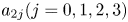$a_{2j} (j=0,1,2,3)$ are given by

(4.20a)$$\begin{gather} a_{20}=15(5+6 \alpha+\alpha^2),\quad a_{21}={-}(225+150 \alpha+167\alpha^2), \end{gather}$$

(4.20b)$$\begin{gather}a_{22}={-}7\alpha(30+13\alpha), \quad a_{23}=63 \alpha^2. \end{gather}$$

Notice that $c_2$ and $\zeta _2$ are proportional to $\gamma =O(\beta ^2)$, as expected.

Similarly, at $O(\beta ^4), c_4$ and $\zeta _4(X)$ that are proportional to $\gamma ^2$ can be found as

(4.21)$$\begin{gather} {c_4\over c_0}={\alpha(40 + 21 \alpha )\over 1400} \gamma^2, \end{gather}$$

(4.22)$$\begin{gather}{\zeta_4\over h} = {\alpha \over 22050000} \left(a_{40} S^2+\sum_{j=1}^6 a_{4j} S^{2j}T^2\right)\gamma^2, \end{gather}$$

where $a_{4j}$ ($j=0,1,\ldots,6$) are given by

(4.23a)$$\begin{gather} a_{40}={-}1050 ({-}1575 -1455 \alpha +1709 \alpha^2 +1843 \alpha^3 + 254 \alpha^4 ), \end{gather}$$

(4.23b)$$\begin{gather}a_{41}={-}2 \alpha(9161775+4616055 \alpha +5599225 \alpha^2 +964278 \alpha^3), \end{gather}$$

(4.23c)$$\begin{gather}a_{42}={-}12403125 -21895650 \alpha -24960330 \alpha^2 +15477950 \alpha^3 + 3116512 \alpha^4 , \end{gather}$$

(4.23d)$$\begin{gather}a_{43}={-}2 \alpha (- 8037225 +37783755 \alpha +39163725 \alpha^2 + 12100858 \alpha^3 ), \end{gather}$$

(4.23e)$$\begin{gather}a_{44}=10 \alpha^2(14635350 + 10836195 \alpha + 2676968 \alpha^2) , \end{gather}$$

(4.23f)$$\begin{gather}a_{45}=70 \alpha^3 (134985 + 125131 \alpha) , \end{gather}$$

(4.23g)$$\begin{gather}a_{46}={-}4469535 \alpha^4. \end{gather}$$

To summarize, the third-order solitary wave solution valid to $O(\beta ^4)$, or $O(\gamma ^2)$, is given, from (4.10) and (4.11), (4.18) and (4.19), and (4.21) and (4.22), by

(4.24)\begin{align} c&=c_0\left[ 1+ {\alpha\over 10}\gamma+{\alpha(21 \alpha +40 )\over 1400}\gamma^2 +O(\gamma^3) \right],\end{align}

(4.25)\begin{align} \zeta &= a \left[S^2 +{1\over 300}(a_{20} S^2+\sum_{j=1}^3 a_{2j} S^{2j}T^2)\gamma\right.\nonumber\\ &\quad +\left.{1\over 22050000} \left(a_{40} S^2+\sum_{j=1}^6 a_{4j} S^{2j}T^2\right) \gamma^2+O(\gamma^3)\right]. \end{align}

When the solitary wave amplitude is defined by $a_s=\zeta (0)$, its relationship with $a$ can be expanded, in terms of $\gamma$, as

(4.26)\begin{equation} a_s= a\left[1+{a_{20}\over 300} \gamma +{a_{40}\over 22050000} \gamma^2 +O(\gamma^3)\right], \end{equation}

which can be inverted to

(4.27)\begin{align} a&= a_s\left[1-{5+6 a_s+a_s^2\over 20}\,\gamma_s \right.\nonumber\\ &\quad +\left.{2100+10215 a_s +14233 a_s^2 + 6941 a_s^3 + 823 a_s^4\over 42000}\, \gamma_s^2 +O(\gamma_s^3)\right], \end{align}

where $\gamma _s=a_s/(1+a_s)$ and $\gamma =\gamma _s-(5+a_s)\gamma _s^2/20+O(\gamma _s^3)$.

Under the small-amplitude assumption of $\alpha =O (\beta ^2)$, after expanding (4.13) in $\alpha$, the third-order solitary wave solution (4.24) and (4.25) can be reduced to the third-order weakly nonlinear solution given by

(4.28a)$$\begin{gather} c_s/(gh)^{1/2}= [ 1+\textstyle{1\over 2}\alpha_s -\textstyle{3\over 20}\alpha_s^2+ \textstyle{3\over 56}\alpha_s^3 +O(\alpha_s^4)], \end{gather}$$

(4.28b)$$\begin{gather}\zeta/h=\alpha_s [S^2-\textstyle{3\over 4}\alpha_s S^2 T^2 +\alpha_s^2 (\textstyle{5\over 8}S^2 T^2- \textstyle{101\over 80}S^4 T^2)+O(\alpha_s^3)], \end{gather}$$

(4.28c)$$\begin{gather}k_s h= (\textstyle{3\over 4})^{1/2}\alpha_s^{1/2} [ 1-\textstyle{5\over 8}\alpha_s+\textstyle{71\over 128} \alpha_s^2+O(\alpha_s^3)], \end{gather}$$

where $\alpha _s=a_s/h$ and we have made the weakly nonlinear approximation to (4.26) to find $\alpha _s=\alpha +\alpha ^2/4+\alpha ^3/8+O(\alpha ^4)$, which can be inverted to

(4.29)\begin{equation} \alpha=\alpha_s-\textstyle{\frac{1}{4}}\alpha_s^2 +O(\alpha_s^4).\end{equation}

The weakly nonlinear solution given by (4.28) was first obtained by Grimshaw (Reference Grimshaw1971).

4.1.3. Comparison of solutions

Figure 2 shows the comparison between the strongly and weakly nonlinear solitary wave solutions along with the fully nonlinear Euler solutions obtained numerically by Longuet-Higgins & Fenton (Reference Longuet-Higgins and Fenton1974) for the solitary wave speed $c$ and its total mass $M$ defined by

(4.30)\begin{equation} M=\int_{-\infty}^\infty \zeta(X)\, {\rm d} X.\end{equation}

As shown in figure 2(a), as the order of approximation increases, the strongly nonlinear solution for the wave speed $c$ approaches the Euler solution and the comparison is reasonable up to $a_s/h= 0.65$, where the difference is less than 1 %. As shown in figure 2(b), a similar conclusion can be made to the total mass $M$, for which the difference is approximately 3 % when $a_s/h=0.65$. Considering that the maximum solitary wave amplitude is approximately $a_s/h= 0.827$, the third-order solitary wave solution can be considered a good approximation to the Euler solution for finite-amplitude solitary waves. The difference increases with the wave amplitude, but this is not so surprising. The solitary wave becomes sharper near the crest as the amplitude increases so that the long wave approximation starts to be locally invalid.

Figure 2. (a) Solitary wave speed $c$ and (b) total mass $M$ vs amplitude $a_s$ for different orders of approximation (dotted: first order; dashed: second order; solid: third order). The black and red lines represent the strongly nonlinear and weakly nonlinear solutions, respectively. The symbols are the numerical solution of the Euler equations from Longuet-Higgins & Fenton (Reference Longuet-Higgins and Fenton1974). In (a), the third-order weakly nonlinear solution for $c$ is close to the third-order strongly nonlinear solution and is not shown here.

In figure 3, the strongly nonlinear solitary wave profiles for $a_s/h=0.460$ are compared with the Euler solutions computed by Li et al. (Reference Li, Hyman and Choi2004). While the first-order solution (or Rayleigh's solution) is wider than the Euler solution, both the second-order and third-order solutions agree well with the Euler solution. While the first- and second-order weakly nonlinear solutions (not shown here) compare poorly with the Euler solution, the third-order weakly nonlinear solution is as good as the third-order strongly nonlinear solution.

Figure 3. Solitary wave profiles for $a_s/h=0.460$. (a) Strongly nonlinear solutions under the first- (dotted), second- (dashed) and third-order (solid) approximations are compared with the numerical solution of the Euler equations (symbols) computed by Li, Hyman & Choi (Reference Li, Hyman and Choi2004).(b) Comparison between the strongly (solid) and weakly (dashed) nonlinear solutions under the third-order approximation. The first- and second-order weakly nonlinear solutions compare poorly with the Euler solutions and are not shown here.

In figure 4, the wave amplitude is further increased to $a_s/h=0.663$. As can be seen in figure 4(a), the comparison of the strongly nonlinear solution with the Euler solution improves as the order of approximation increases. The third-order strongly nonlinear solution is slightly wider than the Euler solution, in particular near the crest, where short-wavelength components are no longer negligible. Away from the crest, the third-order solution agrees well with the Euler solution.

Figure 4. Solitary wave profiles for $a_s/h=0.663$. In (a), strongly nonlinear solutions under the first- (dotted), second- (dashed) and third-order (solid) approximations are compared with the numerical solution of the Euler equations (symbols) computed by Li et al. (Reference Li, Hyman and Choi2004). In (b–d), the strongly nonlinear solutions (solid) are compared with the weakly nonlinear solutions (dashed) under the third-, first-, second-order approximations, respectively. Notice that the comparison of the weakly nonlinear solution with the Euler solution (symbols) depends sensitively on the order of approximation.

In figure 4(b), it is surprising to see that the third-order weakly nonlinear solution compares better with the Euler solution than the strongly nonlinear one, in particular near the crest, even though the amplitude ($a_s/h=0.663$) is too large for the weakly nonlinear theory to be valid. Furthermore, the long wave theory is expected to fail to describe the profile near crest when the wave amplitude is large as the wave slope becomes so steep (eventually to form a corner at the maximum amplitude). As discussed in Murashige & Choi (Reference Murashige and Choi2015) in terms of singularity structures in the complex planes of different theoretical models, this agreement might be coincident. As can be seen in figure 2, the comparison of the weakly nonlinear solution with the Euler solution depends sensitively on the order of nonlinearity while that of the strongly nonlinear solution improves uniformly with the order. In addition, the strongly nonlinear solution better behaves on the outskirts of the solitary wave, where the long wave approximation should be applicable. This can be also seen in figure 4(c,d), where the Euler solution is compared with first- and second-order solutions. The weakly nonlinear solution near the crest agrees well with the Euler solution under the first-order approximation, but compares poorly under the second-order approximation. On the other hand, irrespective of the order of approximation, the strongly nonlinear solitary wave solution (4.25) shows uniform convergence to the Euler solution and can be used reliably. Furthermore, as shown later in figure 5, the weakly nonlinear solutions for finite-amplitude waves are no longer valid when their velocity profiles are compared with the Euler solutions.

Figure 5. Horizontal velocity profile $U(z)$ below the crest of a solitary wave for (a) $a_s/h=0.215$; (b) $a_s/h=0.310$; (c) $a_s/h=0.428$; (d) $a_s/h=0.65$. The third-order solution (solid) is compared with the second-order solution (dashed), the third-order weakly nonlinear solution (dot-dashed) given by (4.38), the numerical solution of the level-4 GN model of Zhao et al. (Reference Zhao, Ertekin, Duan and Hayatdavoodi2014) (circles) and the numerical solution of Tanaka (Reference Tanaka1986) shown in Madsen et al. (Reference Madsen, Bingham and Liu2002) (squares). Notice that the first-order solution (dotted) is independent of $z$.

4.2. Velocity and pressure fields induced by a solitary wave

The velocity and pressure fields induced by a solitary wave is of great interest for applications. After the $M$th-order solitary wave solution is found, one should find the corresponding velocity and pressure fields with care so that their expressions are asymptotically consistent with the solitary wave solution. Otherwise, the results contain higher-order terms that have been neglected for the solitary wave solution and could show poor agreement with the Euler solutions.

4.2.1. Velocity fields

The horizontal and vertical velocities, $(u,w)=(\phi _X, \phi _z)$, induced by a solitary wave can be computed, from (2.26), as

(4.31)$$\begin{gather} u(X, z)=\sum_{m=0}^\infty {({-}1)^m\over (2m)!} (z+h)^{2m} D^{2m} v, \end{gather}$$

(4.32)$$\begin{gather}w(X, z)=\sum_{m=0}^\infty {({-}1)^{m+1}\over (2m+1)!} (z+h)^{2m+1} D^{2m+1} v, \end{gather}$$

where $-h\le z\le \zeta$. To find an asymptotically consistent velocity field, the bottom velocity $v(X)=D\phi _b$ should be first expanded as

(4.33)\begin{equation} v=\sum_{m=0}^\infty v_{2m}^s,\end{equation}

where $v_{2m}^s=O(\beta ^{2m})$ can be found by substituting into (4.2) the expansions for $\zeta$ and $c$ given by (4.14). For example, up to the third order, $v_{2m}^s$ ($m=0,1,2$) can be explicitly found as

(4.34a)\begin{align} v_0^s&= {c_0 \zeta_0\over \eta_0}, \end{align}

(4.34b)\begin{align} v_2^s&={c_2 \zeta_0\over \eta_0} +{c_0h\over 6\eta_0^2}[ 6\zeta_2 +\eta_0 ({-}2{\zeta_0'}^2+\eta_0\zeta_0'')], \end{align}

(4.34c)\begin{align} v_4^s&={c_4 \zeta_0\over \eta_0} +{c_2h\over 6\eta_0^2}[ 6\zeta_2 +\eta_0({-}2{\zeta_0'}^2+ \eta_0\zeta_0'')]\nonumber\\ &\quad +{c_0h\over 360 \eta_0^3}[ 360 \eta_0\zeta_4-360 \zeta_2^2+120 \eta_0{\zeta_0'}^2\zeta_2 -240 \eta_0^2\zeta_0'\zeta_2'+60 \eta_0^3\zeta_2''\nonumber\\ &\quad +\eta_0^2(32\,{\zeta_0'}^4-8 \eta_0{\zeta_0'}^2\zeta_0''-22 \eta_0^2 {\zeta_0''}^2 -16 \eta_0^2\zeta_0'\zeta_0'''+7 \eta_0^3\zeta_0'''')], \end{align}

where the expressions for $\zeta _{2m}$ and $c_{2m}$ have been obtained in § 4.1. Then, after substituting (4.33) into (4.31) and (4.32), one can find the following expressions for $u$ and $w$

(4.35a,b)$$\begin{gather} u(X,z)=\sum_{m=0}^\infty u_{2m}^s(X,z),\quad u_{2m}^s=\sum_{j=0}^m \frac{({-}1)^j}{(2j)!} (z+h)^{2j} D^{2j} v_{2(m-j)}^s, \end{gather}$$

(4.36a,b)$$\begin{gather}w(X,z)=\sum_{m=0}^\infty w_{2m}^s(X,z),\quad w_{2m}^s=\sum_{j=0}^m \frac{({-}1)^{j+1}}{(2j+1)!} (z+h)^{2j+1} D^{2j+1} v_{2(m-j)}^s, \end{gather}$$

where $u_{2m}^s$ and $w_{2m}^s$ are both $O(\beta ^{2m})$. The horizontal velocity profile below the solitary wave crest is also of interest and can be found as $U(z)=u(0,z)$ as

(4.37)\begin{align} U(z)/(gh)^{1/2}&={\alpha\over (1+\alpha)^{1/2}} \left[1 +\left \{- {\alpha\over 10} +{3\over 4}{(1+z/h)^2\over 1+\alpha}\right \} \gamma \right. \nonumber\\ &\quad +\left\{- \frac{\alpha(5820+8519 \alpha+3194 \alpha^2)}{21000} +\frac{3\alpha(1+6\alpha)}{40}{(1+z/h)^2\over 1+\alpha} \right.\nonumber\\ &\quad \left.\left. +\frac{3(2-\alpha)}{16}{(1+z/h)^4\over (1+\alpha)^2} \right\}\gamma^2 +O(\gamma^3) \right], \end{align}

from which the horizontal velocity at the crest $U_c$ can be obtained as $U_c=U(a_s)$.

By expanding (4.37) for small $\alpha _s$, the weakly nonlinear solution correct to the third order in $\alpha _s$ can be obtained as

(4.38)\begin{align} {U}(z)/(gh)^{1/2}&=\alpha_s+\textstyle{\frac{3}{4}}\alpha_s^2[{-}1+ (1+z/h)^2]\nonumber\\ &\quad +\alpha_s^3[\textstyle{\frac{21}{40}} - \textstyle{\frac{9}{4}} (1+z/h)^2 +\textstyle{\frac{3}{8}} (1+z/h)^4]+O(\alpha_s^4). \end{align}

The horizontal velocity at the crest $U_c=U(a_s)$ is given, after neglecting terms of $O(\alpha _s^4)$, by

(4.39)\begin{equation} {U_c}/(gh)^{1/2}=\alpha_s+\textstyle{\frac{3}{20}} \alpha_s^3+O(\alpha_s^4).\end{equation}

These third-order weakly nonlinear solutions given by (4.38) and (4.39) are identical to those in Grimshaw (Reference Grimshaw1971).

In figure 5, the vertical profile of the horizontal velocity below the solitary wave crest $U(z)$ is computed for $a_s/h=0.65$ and is compared with the numerical solution of the Euler equations of Tanaka (Reference Tanaka1986), which was also confirmed by Madsen et al. (Reference Madsen, Bingham and Liu2002). Once again, the third-order strongly nonlinear solution for the horizontal velocity profile shows good agreement with the Euler solution. It is interesting to notice that there is a considerable discrepancy between the third-order weakly nonlinear solution given by (4.38) and the Euler solution for the velocity profile although the two solutions agree well for the wave profile. This shows that an asymptotic result should be used with care, in particular, when it is applied to a parameter range outside its validity. Figure 6 shows the horizontal velocity at the crest of the solitary wave $U_c$ vs $a_s$. Compared with the first-order solution (Rayleigh's solution), the third-order solution shows considerable improvement in the comparison with the Euler solution of Tanaka (Reference Tanaka1986).

Figure 6. The particle velocity at the crest $U_c$ vs the solitary wave amplitude $a_s$. The first (dotted), second (dashed) and third-order (solid) strongly nonlinear solutions are compared with the numerical solution of the Euler equations of Tanaka (Reference Tanaka1986) (symbols) as well as the third-order weakly nonlinear solution (dot-dashed).

4.2.2. Pressure field

Using the Bernoulli equation given by

(4.40)\begin{equation} p ={-} \rho \left[gz+ {\partial \phi\over \partial t}+\frac12 (u^2 +w^2) \right] ,\end{equation}

the pressure field $p(\boldsymbol x,z,t)$ can be found as

(4.41)\begin{equation} p(\boldsymbol x,z,t)={-}\rho gz+\sum_{m=0}^\infty p_{2m}(\phi_b, z),\end{equation}

where $p_{2m}$ are given, from (2.6a) and (4.35) and (4.36), by

(4.42)\begin{align} p_{2m}&=\rho({-}1)^{m+1} (z+h)^{2m} \left[ {1\over (2m)!} {\partial \over\partial t} (D^{2m-1} v )\right.\nonumber\\ &\quad +\frac12 \sum_{l=0}^m \left \{ {1 \over (2 l)! (2(m-l))!} (D^{2 l}v) ( D^{2(m-l)}v)\right.\nonumber\\ &\quad \left.\left.+{(z+h)^2\over (2 l+1)! (2(m-l)+1)!} (D^{2 l+1}v)(D^{2(m-l)+1}v )\right \} \right]. \end{align}

In a frame of reference moving with a solitary wave, the dynamic bottom pressure defined by $P(X) = p(X, -h)-\rho g h$ is given, from (4.40), by

(4.43)\begin{equation} P(X)= p_0(\phi_b, -h)= \rho (c v-\tfrac12 v^2),\end{equation}

which can be also found from (4.41) with $p_{2m}=0$ at $z=-h$ for $m\ne 0$. To compute the dynamic bottom pressure, the expansion for $v$ given by (4.33) is substituted into (4.43) and is re-arranged to have

(4.44a,b)\begin{equation} P(X)=\sum_{m=0}^\infty P_{2m}^s(X), \quad P_{2m}^s(X)=\rho \sum_{j=0}^m \left(c_{2m}v_{2(m-j)}^s-\frac12 v_{2m}^sv_{2(m-j)}^s\right). \end{equation}

In particular, to the third order in $\gamma$, the bottom pressure below the crest of the solitary wave $P_c=P(0)$ is given by

(4.45)\begin{equation} {P_c\over \rho g h}=\frac{2+\alpha}{2}\, \gamma +{\frac{\alpha^2}{10}}\,\gamma^2 -\frac{\alpha}{10500}(2610+3907 \alpha+1597 \alpha^2)\gamma^3+O (\gamma^4).\end{equation}

Under the weakly nonlinear assumption, the expression of $P_c$ in (4.45) can be reduced to

(4.46)\begin{equation} {P_c\over \rho g h}=\alpha_s-\textstyle{\frac{3}{4}}\alpha_s^2+ \textstyle{\frac{3}{4}}\alpha_s^3+O(\alpha_s^4),\end{equation}

where (4.29) has been used for the expression of $\alpha _s$ in terms of $\alpha$. This third-order weakly nonlinear result was found previously by Fenton (Reference Fenton1972).

Figure 7 shows the variation of the bottom pressure $P_c$ with the wave amplitude $a_s$. Compared with the third-order strongly nonlinear solution given by (4.45), the lower-order solutions as well as the third-order weakly nonlinear solution over-predicts the bottom pressure $P_c$ when the wave amplitude is finite.

Figure 7. Bottom pressure below the wave crest $P_c$ vs the solitary wave amplitude $a_s$. The third-order solution (solid) is compared with the first- (dotted) and second-order (dashed) solutions as well as the third-order weakly nonlinear solution (dot-dashed) of Grimshaw (Reference Grimshaw1971).

5.1. First-order model

When the leading-order dispersive terms of $O(\beta ^2)$ are included, (5.1) can be reduced to the first-order ($M=1$) system given by

(5.5a)$$\begin{gather} \zeta_t+\boldsymbol{\nabla}{{\boldsymbol \cdot}} \left[\left(\eta-{\eta^3\over 3!}\nabla^2\right) \boldsymbol{\nabla}\phi_b\right]=0, \end{gather}$$

(5.5b)$$\begin{gather}\left[ \left(1-{\eta^2\over 2!}\nabla^2\right)\phi_b\right]_t +g\zeta+{1\over 2}\boldsymbol{\nabla}\phi_b{{\boldsymbol \cdot}} \boldsymbol{\nabla}\phi_b = \boldsymbol{\nabla}{{\boldsymbol \cdot}}\left( {\eta^2\over 2!}\nabla^2\phi_b \boldsymbol{\nabla}\phi_b\right), \end{gather}$$

which is the system derived by Wei et al. (Reference Wei, Kirby, Grilli and Subramanya1995) for the bottom velocity potential. For weakly nonlinear waves of $\alpha =O(\beta ^2)$, this first-order system can be further reduced to the first-order weakly nonlinear model

(5.6a)$$\begin{gather} \zeta_t+ \boldsymbol{\nabla}{{\boldsymbol \cdot}} [(h+\zeta)\boldsymbol{\nabla}\phi_b]-{h^3\over 3!} (\nabla^2)^2\phi_b =0, \end{gather}$$

(5.6b)$$\begin{gather}\left( 1-{h^2\over 2!}\nabla^2 \right){\phi_b}_t +g\zeta+{1\over 2}\boldsymbol{\nabla}\phi_b{{\boldsymbol \cdot}} \boldsymbol{\nabla}\phi_b=0 , \end{gather}$$

which was first obtained by Mei & Le Méhaute (Reference Mei and Le Méhaute1966).

After taking the gradient, the first-order system (5.5) can be written, in terms of the bottom velocity $\boldsymbol v=\boldsymbol {\nabla }\phi _b$, as

(5.7a)$$\begin{gather} \zeta_t+\boldsymbol{\nabla}{{\boldsymbol \cdot}} \left[\left(\eta-{\eta^3\over 3!} \nabla^2\right)\boldsymbol v\right]=0, \end{gather}$$

(5.7b)$$\begin{gather}\left[ \boldsymbol v-\boldsymbol{\nabla} \left({\eta^2\over 2!}\boldsymbol{\nabla}{{\boldsymbol \cdot}} \boldsymbol v\right)\right]_t+\boldsymbol{\nabla} \left(g\zeta+{1\over 2} \boldsymbol v{{\boldsymbol \cdot}} \boldsymbol v\right) = \boldsymbol{\nabla} \left[\boldsymbol{\nabla}{{\boldsymbol \cdot}}\left \{ {\eta^2\over 2!} (\boldsymbol{\nabla}{{\boldsymbol \cdot}}\boldsymbol v) \boldsymbol v\right \}\right]. \end{gather}$$

This system is asymptotically equivalent to the strongly nonlinear long wave model for the depth-averaged velocity, or the SG/GN equations. Using the relationship between the bottom velocity $\boldsymbol v$ and the depth-averaged velocity $\bar {\boldsymbol u}$ given, from (3.11), by

(5.8)\begin{equation} \boldsymbol v = \bar{\boldsymbol u}+{\eta^2\over 3!} \nabla^2\bar{\boldsymbol u}+O(\beta^4), \end{equation}

equation (5.7a) becomes (3.10) while (5.7b) can be written as

(5.9)\begin{equation} \left[\bar{\boldsymbol u}-{1\over \eta}\boldsymbol{\nabla}\left({\eta^3\over 3}\boldsymbol{\nabla}{{\boldsymbol \cdot}} \bar{\boldsymbol u}\right)\right]_t +\boldsymbol{\nabla}\left(g\zeta +{1\over 2} \bar{\boldsymbol u}{{\boldsymbol \cdot}}\bar{\boldsymbol u}\right) =\boldsymbol{\nabla} \left[{\eta^2\over 2} ( \boldsymbol{\nabla}{{\boldsymbol \cdot}} \bar{\boldsymbol u} )^2 +{\bar{\boldsymbol u}\over \eta}{{\boldsymbol \cdot}} \boldsymbol{\nabla} \left({\eta^3\over 3}\boldsymbol{\nabla}{{\boldsymbol \cdot}} \bar{\boldsymbol u}\right) \right].\end{equation}

Here, we have used $\boldsymbol {\nabla }(\boldsymbol {\nabla }{{\boldsymbol \cdot }} \bar {\boldsymbol u})=\nabla ^2 \bar {\boldsymbol u}+O(\beta ^2)$. This scaling can be seen from (3.12), or

(5.10)\begin{equation} \boldsymbol{\nabla}\times \bar{\boldsymbol u}={-}\textstyle\frac{1}{3} (\eta\boldsymbol{\nabla} \eta\times \nabla^2 \bar{\boldsymbol u})+O (\beta^4) = O(\beta^2).\end{equation}

After rearranging terms and using (5.10), one can show that (5.9) along with (3.10) yields the SG/GN equations for the depth-averaged velocity $\bar {\boldsymbol u}$

(5.11a,b)\begin{align} \zeta_t+\boldsymbol{\nabla}{{\boldsymbol \cdot}} (\eta\bar{\boldsymbol u})=0,\quad \bar{\boldsymbol u}_t+\bar{\boldsymbol u}{{\boldsymbol \cdot}}\boldsymbol{\nabla} \bar{\boldsymbol u}+g\boldsymbol{\nabla}\zeta = \frac{1}{\eta}\boldsymbol{\nabla} \left[ \frac{\eta^3}{3} \{ \boldsymbol{\nabla}{{\boldsymbol \cdot}} \bar{\boldsymbol u}_t +\bar{\boldsymbol u}{{\boldsymbol \cdot}}\boldsymbol{\nabla} (\boldsymbol{\nabla}{{\boldsymbol \cdot}} \bar{\boldsymbol u})-(\boldsymbol{\nabla}{{\boldsymbol \cdot}} \bar{\boldsymbol u})^2 \} \right].\end{align}

For one-dimensional waves, Rayleigh's solution given by (4.11) is the solitary wave solution of (5.11), as pointed out earlier, with $\bar u= c (\zeta /\eta )$.

5.2. Second-order model

The second-order ($M=2$) model correct to $O(\beta ^4)$ can be written explicitly as

(5.12a)\begin{align} &\zeta_t+\boldsymbol{\nabla}{{\boldsymbol \cdot}} \left[\left\{\eta-{\eta^3\over 3!}\nabla^2+ {\eta^5\over 5!}(\nabla^2)^2\right\}\boldsymbol{\nabla}\phi_b\right]=0, \end{align}

(5.12b)\begin{align} &\left[ \left\{ 1-{\eta^2\over 2!}\nabla^2+{\eta^4\over 4!}(\nabla^2)^2 \right\} \phi_b \right]_t+g\zeta+{1\over 2}\boldsymbol{\nabla}\phi_b{{\boldsymbol \cdot}} \boldsymbol{\nabla}\phi_b\nonumber\\ &\quad = \boldsymbol{\nabla}{{\boldsymbol \cdot}}\left({\eta^2\over 2!} \nabla^2\phi_b \boldsymbol{\nabla}\phi_b\right)-\boldsymbol{\nabla}{{\boldsymbol \cdot}}\left[{\eta^4\over 4!} \{\nabla^2 (\nabla^2 \phi_b \boldsymbol{\nabla}\phi_b) +\boldsymbol{\nabla}(\nabla^2\phi_b)^2 \}\right] . \end{align}

The truncated total energy correct to $O (\beta ^4 )$ is given by $E=E_0+E_2+E_4$ with 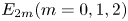$E_{2m} (m=0,1,2)$ defined, from (3.15) and (3.16), by

(5.13a)$$\begin{gather} E_0= {1\over 2!} \int ( g\zeta^2+ \eta\boldsymbol{\nabla}\phi_b {{\boldsymbol \cdot}}\boldsymbol{\nabla}\phi_b) \,{\rm d} \boldsymbol x, \end{gather}$$

(5.13b)$$\begin{gather}{E}_{2}={1\over 3!} \int\eta^3 [(\nabla^2\phi_b)^2 -\boldsymbol{\nabla} \phi_b{{\boldsymbol \cdot}}\nabla^2\boldsymbol{\nabla}\phi_b]\, {\rm d} {\boldsymbol x}, \end{gather}$$

(5.13c)$$\begin{gather}E_4={1\over 5!}\int \eta^5 [3\nabla^2(\boldsymbol{\nabla}\phi_b){{\boldsymbol \cdot}} \nabla^2(\boldsymbol{\nabla}\phi_b)-4(\nabla^4\phi_b)(\nabla^2\phi_b)+\boldsymbol{\nabla} \phi_b{{\boldsymbol \cdot}}\nabla^4\boldsymbol{\nabla}\phi_b ]\, {\rm d} {\boldsymbol x}. \end{gather}$$

As mentioned previously, unlike the system for the surface velocity potential and that for the depth-averaged velocity, it can be shown that the system given by (5.12) conserves the truncated total energy only asymptotically. Likewise, the second-order solitary wave solution obtained in § 4 is only the asymptotic solution of the second-order system (5.12).

5.3. Truncated model with the full linear dispersion relation

The truncated system (5.1) for the bottom velocity is always well-posed at any order of approximation, but the linear dispersion relation of a lower-order model is inaccurate, in particular, for short waves. While the system is supposed to correctly describe only long waves, one cannot avoid short waves excited by, for example, numerical errors, nonlinearity and bottom variation. Following Whitham (Reference Whitham1974), the truncated system (5.1) can be modified to include the full linear dispersion relation as

(5.14a)$$\begin{gather} \zeta_t ={-}{\mathcal{L}} [{\phi_b} ] +\left[\left(\sum_{m=0}^M {Q}_{2m}\right)- {\mathcal{S}}_{2M} [\phi_b ]\right], \end{gather}$$

(5.14b)$$\begin{gather}\left[\phi_b +\left(\sum_{m=1}^M {\varPhi}_{2m}\right) - {\mathcal{C}}_{2M} [\phi_b ]\right]_t=\sum_{m=0}^M {R}_{2m} , \end{gather}$$

where the Fourier transform of an integral operator ${\mathcal {L}}[\phi _b]$ is defined, from (2.5), as $\widehat {{\mathcal {L}}[\phi _b]}= - (k\tanh kh) \hat \phi _b$ so that $W\simeq -{\mathcal {L}}[\phi _b]$. Here, the local operators ${\mathcal {S}}_{2M}$ and ${\mathcal {C}}_{2M}$ defined in (5.3) are introduced to eliminate the truncated linear dispersion relation while ${\mathcal {L}}[\phi _b]$ provides the full linear dispersion relation: $\omega ^2=gk\tanh kh$. This idea was first proposed by Whitham (Reference Whitham1974), who replaced the third-order spatial derivative term in the KdV equation by an integral operator that produces the full linear dispersion relation for uni-directional waves. Nevertheless, it should be remarked that the system given by (5.14) is asymptotically inconsistent and needs to be carefully tested prior to its application. Furthermore, the high-order nonlinearity in the strongly nonlinear long wave model along with the full dispersive terms could increase the wave steepness (Whitham Reference Whitham1974), which makes computations challenging. Even for ill-posed systems, the (unstable) linear terms can be replaced by the same non-local term to regularize the systems (Choi Reference Choi2019), but the issues mentioned above cannot be avoided. Therefore, care should be taken in using the regularized strongly nonlinear model (5.14) until the interplay between high-order nonlinearity and full dispersion is fully understood.

6.1. Finite difference approximation to the linearized first-order system

After all physical variables are non-dimensionalized with respect to $h$ and $g$ (or, equivalently, $h=g=1$ are chosen), the linearized system for $\zeta$ and $v$ given, from (6.2), by

(6.3a,b)\begin{equation} \zeta_t+v_x-{\textstyle\frac{1}{6}} v_{xxx}=0,\quad (v-\tfrac{1}{2} v_{xx})_t+\zeta_x=0,\end{equation}

can be approximated, using the second-order central difference scheme in space, as

(6.4a,b)\begin{equation} \zeta_t+D_0v-{\textstyle{1\over 6}} D_0D_+D_-v=0,\quad (v-{\textstyle{1\over 2}} D_+D_-v)_t+D_0\zeta =0.\end{equation}

Here, $D_+, D_-$ and $D_0$ are the forward, backward and central differences, respectively, so that the finite difference approximations for the first-, second- and third-order derivatives are given by

(6.5a)$$\begin{gather} D_0 v_j= {v_{j+1}-v_{j-1}\over 2\Delta x}={v_{x}}_j + {\Delta x^2\over 6}{v_{xxx}}_j +O(\Delta x^4), \end{gather}$$

(6.5b)$$\begin{gather}D_+D_-v_j = {v_{j+1}-2v_j+v_{j-1}\over \Delta x^2}={v_{xx}}_j +{\Delta x^2\over 12}{v_{xxxx}}_j+O(\Delta x^4), \end{gather}$$

(6.5c)$$\begin{gather}D_0D_+D_-v_j = {v_{j+2}-2v_{j+1}+2v_{j-1}-v_{j-2}\over 2\Delta x^3} ={v_{xxx}}_j +{\Delta x^2\over 4}{v_{xxxxx}}_j+O(\Delta x^4), \end{gather}$$

where $\Delta x$ is the grid size and $v_j=(x_j,t)$ with $x_j=j\Delta x$. Notice that the terms proportional to $\Delta x^2$ in (6.5) represent the leading-order truncation errors associated with the central difference approximation adopted here and can be found by expanding $v_{j\pm 1}$ and $v_{j\pm 2}$ for small $\Delta x$ about $x=x_j$.

With these finite difference approximations, the linear system (6.3) is modified to

(6.6a)$$\begin{gather} \zeta_t+v_x-{1\over 6}(1-\Delta x^2) v_{xxx}-{\Delta x^2\over 24} v_{xxxxx}=O(\Delta x^4), \end{gather}$$

(6.6b)$$\begin{gather}\left(v-{1\over 2}v_{xx} -{\Delta x^2\over 24} v_{xxxx}\right)_t+ \zeta_x +{\Delta x^2\over 6} \zeta_{xxx} =O(\Delta x^4), \end{gather}$$

whose linear dispersion relation can be obtained as

(6.7)\begin{align} \omega^2=k^2\left.\left( 1-{\Delta x^2\over 6}k^2\right) \left[ 1+{1\over 6}k^2-{\Delta x^2\over 6}k^2 \left(1+{1\over 4}k^2\right) \right]\right/ \left( 1+ {1\over 2}k^2- {\Delta x^2\over 24} k^4 \right),\end{align}

which can be reduced to (2.16) with $M=1$ as $\Delta x\to 0$. The question is if the right-hand side of (6.7) is always positive when $\Delta x$ is small, but non-zero. If not, $\omega$ is purely imaginary for a certain range of $k$ and the finite difference scheme would then be unstable to disturbances whose wavenumbers are within the range. Notice that the denominator of (6.7) is always positive for $0\le k\le k_{max}$, where $k_{max}$ is the maximum wavenumber resolved by a finite difference scheme given by $k_{max}={\rm \pi} /\Delta x$. Then, the sign of the right-hand side of (6.7) follows that of its numerator, from which the range of $\bar k =k\Delta x$ for imaginary $\omega$ or numerical instability can be approximated by $2<\bar k<\sqrt {6}\simeq 2.449$ for small $\Delta x$. This implies that, when the system given by (6.2) is discretized, the disturbances whose wavenumbers are within this range can be unstable when they are excited. As the growth rate in (6.7) is proportional to $1/\Delta x$ with $\bar k=O(1)$, the numerical scheme becomes more unstable when $\Delta x$ is decreased to obtain a more accurate solution.

It should be recalled that this difficulty arises from the finite difference approximation of high-order spatial derivatives in (6.2) even though the system is well-posed. This discussion can be also applied to the weakly nonlinear model for the bottom variable although its nonlinear behaviour would be different from its strongly nonlinear counterpart.

On the other hand, the first-order or SG/GN equations for the depth-averaged velocity ${\bar u}$ is given, from (A10) after dropping terms of $O(\beta ^4)$, by

(6.8a,b)\begin{align} \zeta_t+(\eta \bar{u})_x=0,\quad \left[\bar{u}-\frac{1}{3\eta}({\eta^3} \bar{u}_x)_x\right]_t +g\zeta_x +\bar{u}\,\bar{u}_x =\left[\frac{\eta^2}{2}{\bar{u}_x}^2 +\frac{\bar{u}}{\eta}\left(\frac{\eta^3}{3} \bar{u}_x\right)_x \, \right]_x.\end{align}

When the SG/GN equations are linearized and discretized using the previous second-order finite difference scheme, they can be modified to

(6.9a)$$\begin{gather} \zeta_t+{\bar u}_x+{\Delta x^2\over 6} {\bar u}_{xxx}=O(\Delta x^4), \end{gather}$$

(6.9b)$$\begin{gather}\left({\bar u}-\frac{1}{3}{\bar u}_{xx} -{\Delta x^2\over 36}{\bar u}_{xxxx}\right)_t+\zeta_x +{\Delta x^2\over 6}\zeta_{xxx} =O(\Delta x^4), \end{gather}$$

whose dispersion relation can be found as

(6.10)\begin{equation} \omega^2=\left. {k^2\left(1-{\Delta x^2\over 6}k^2\right)^2}\right/ \left(1+\frac{1}{3}k^2-{\Delta x^2\over 36} k^4\right). \end{equation}

The right-hand side of (6.10) can be shown always positive for $0< k< k_{max}$ for any choice of $\Delta x$ and, unlike that for the bottom velocity $v$, the modified system for the depth-averaged velocity ${\bar u}$ is always neutrally stable with the second-order central difference approximation. Furthermore, unlike that given by (6.7), the frequency $\omega$ given by (6.10) for the depth-averaged system is independent of $\Delta x$ and is bounded as $\Delta x\to 0$, which implies the system given by (6.8) imposes little constraint on the choice of $\Delta t$ for numerical stability. Therefore, the system for the depth-averaged velocity is more suitable for numerical computations than that for the bottom variable. Unfortunately, the issue of the depth-averaged system is that it could be ill-posed when truncated at even orders in $\beta ^2$.

While we only consider the first-order system, the similar numerical issues discussed previously are expected to appear in the higher-order systems for the bottom velocity. As the order of approximation increases, we need to include higher-order spatial derivatives, which would make the corresponding modified system more unstable. This indicates that finite difference approximations might not be so suitable to solve the strongly nonlinear system for the bottom velocity given by (6.1) or (6.2). Therefore, we adopt a pseudo-spectral method, with which high-order spatial derivatives can be accurately evaluated.

6.2. Pseudo-spectral method for the second-order system

To solve (6.1), we use a pseudo-spectral method based on Fourier series, where $\zeta$ and $v$ are approximated by finite complex Fourier series

(6.11a,b)\begin{equation} \zeta(x,t) = \sum_{n={-}N/2+1}^{N/2} {\hat \zeta}_n(t)\, {\rm e}^{{\rm i} k_n x},\quad v(x,t) = \sum_{n={-}N/2+1}^{N/2} {\hat v}_n(t)\, {\rm e}^{{\rm i} k_n x}, \end{equation}

where $N$ is the total number of Fourier modes for computations and $k_n=2{\rm \pi} n/L$ with $L$ being the computational domain length. We use a fast Fourier transform routine to compute the complex Fourier coefficients $(\hat \zeta _n,\hat v_n)$ for $-N/2+1\le n\le N/2$ defined by

(6.12a,b)\begin{equation} \hat \zeta_n(t)=\sum_{j=0}^{N-1} \zeta_j(t) \,{\rm e}^{-{\rm i} k_n x_j}, \quad \hat v_n(t)=\sum_{j=0}^{N-1} v_j(t) \,{\rm e}^{-{\rm i} k_n x_j},\end{equation}

where $\zeta _j(t)= \zeta (x_j,t)$ and $v_j(t)= v(x_j,t)$ with $x_j=j\Delta x (j=0,\ldots, N-1)$. When linearized, (6.1) yields a coupled system of ordinary differential equations for $\hat \zeta _n(t)$ and $\hat v_n(t)$, from which one can find the dispersion relation given by (2.16) with $M=2$. In solving (6.1), the spatial derivatives are evaluated in Fourier space while the nonlinear terms are computed in physical space. Then, the evolution equations in (6.1) are integrated in time using the fourth-order Runge–Kutta (RK4) scheme.

At every time step when a nonlinear system is solved numerically with finite Fourier series, aliasing errors are introduced and a filter needs to be applied to eliminate them. As the order of nonlinearity $M_{NL}$ is given by $M_{NL}=2M+2$, with $M$ being the order of approximation, one can in principle eliminate the aliasing errors by removing the Fourier coefficients $\hat \zeta _n$ and $\hat v_n$ for $\vert n\vert >[(M_{NL}-1) /(M_{NL}+1)] (N/2)$ so that we only keep the Fourier modes for $\vert n\vert >[2 /(M_{NL}+1)]\,(N/2)$. Although the total energy is conserved only asymptotically for (6.1), it is monitored to make sure that the de-aliasing filter produces no significant energy loss.

After solving (6.1a) for $\zeta$ and (6.1b) for $\varPhi _x$ given by

(6.13)\begin{equation} \varPhi_x = v-\left({\eta^2\over 2!}v_{x}-{\eta^4\over 4!}v_{xxx} \right)_x , \end{equation}

one needs to invert (6.13) to find $v$ at a new time step. A similar inversion step was required to solve the regularized two-layer long wave model for internal waves proposed by Choi, Barros & Jo (Reference Choi, Barros and Jo2009), for which an iterative scheme was developed for the inversion (Choi, Goullet & Jo Reference Choi, Goullet and Jo2011). Here, we adopt a similar iterative scheme, which can be written as

(6.14)\begin{equation} \left(1-{\xi^2\over 2!}\partial_x^2+{\xi^4\over 4!}\partial_x^4\right) v^{(n+1)} =\varPhi_x+ \left[\left({\eta^2\over 2!}-{\xi^2\over 2!}\right)v_{x}^{(n)} -\left({\eta^4\over 4!} -{\xi^4\over 4!} \right)v_{xxx}^{(n)}\right]_x,\end{equation}

where $v^{(n)}$ is the estimate after the $n$th iteration step ($n\ge 0$), $v^{(0)}$ is an initial guess and $\xi$ is a numerical parameter to accelerate the convergence of this iteration scheme, which is chosen to be $\xi =\eta _{max}$, as discussed in Appendix C. After the right-hand side of (6.14) is evaluated in physical space, the linear operator with constant coefficients on the left-hand side can be easily inverted in Fourier space. This iterative scheme is repeated until $\vert \vert v^{(n+1)}-v^{(n)}\vert \vert _{\infty }/\vert \vert v^{(n)}\vert \vert _{\infty }< 10^{-14}$ is satisfied, where $||v^{(n)} ||_{\infty }$ denotes the maximum of $\vert v_{j}^{(n)}\vert$ for $j=1,\ldots, N$.

Alternatively, one can use (3.7) to find the following approximate expression for $v$ in terms of two known functions, $\eta (=h+\zeta )$ and $\varPhi _x$,

(6.15)\begin{equation} v\simeq v_{0}+v_{2}+v_{4}=\varPhi_x+\left({\eta^2\over 2!}\varPhi_{xx}\right)_x -\left[{\eta^2\over 2!}\left({\eta^2\over 2!}\varPhi_{xx}\right)_{xx} -{\eta^4\over 4!}\varPhi_{xxxx}\right]_x.\end{equation}

As this is the asymptotic inversion of (6.13) with an error of $O(\beta ^6)$, the numerical inversion with the iterative scheme given by (6.14) is more preferable as $\beta$ increases. In the meantime, (6.15) is used to find an initial guess for $v$ to start the iteration in (6.14).

In our computations, the steady solitary wave solution of the Euler equations obtained in § 4 is chosen for the initial condition for $\zeta$ while the steady form of (6.1a), or

(6.16)\begin{equation} \left(1-{\eta^2\over 3!} \partial_x^2+{\eta^4\over 5!} \partial_x^4\right) v = {c \zeta\over \eta}, \end{equation}

is used to find the initial condition for $v$ using an iterative scheme similar to (6.14).

Figure 8 shows the numerical solution of the first-order system (6.2) for the propagation of a solitary wave for two different amplitudes: $a=0.2$ and $0.4$. Notice that $a_s=a$ for the first-order solution. The total computational domain is given by $-200\le x \le 200$ although the solution is shown over $-50\le x \le 50$. The number of Fourier modes is $N=(5/2)\times 2^9$ so that $2^9$ Fourier modes are meaningful after applying the de-aliasing filter. The time step is chosen to be $\Delta t =0.1$, which satisfies the stability condition for the RK4 scheme. At $t=200$, the loss of the truncated total energy $E=E_0+E_2+O(\beta ^4)$ defined by (3.16) is approximately 0.199 % and 1.703 % for $a=0.2$ and 0.4, respectively. It should be remembered that the truncated total energy is conserved only asymptotically. As the numerical model runs smoothly, the system for the bottom velocity is confirmed to remain stable when the pseudo-spectral scheme is used. However, as the first-order solitary wave solution of the Euler equations given by (4.11) is not the exact steady solution of the first-order system (6.2), it sheds small-amplitude waves for initial adjustment. For the initial condition for $v$, instead of solving numerically (6.16), one can choose $v_0^s$ given by (4.34a), but the duration for the initial adjustment increases. It is observed that the amplitude of dispersive tails for $a=0.4$ is greater than that for $a=0.2$, which implies that the first-order approximation might not be sufficient enough to describe the solitary wave of $a=0.4$.

Figure 8. Numerical solutions of the first-order system (6.2) for the propagation of a solitary wave of (a) $a/h=0.2$ and (b) $a/h=0.4$. The initial condition for $\zeta$ is given by the first-order solitary solution (4.11) while that for $v$ is found by solving numerically (6.16) without the last term on the left-hand side. The time evolution of the surface elevation $\zeta$ is shown for $0\le t(g/h)^{1/2} \le 200$ in a frame of reference moving with the solitary wave speed $c_0$ defined by (4.10).

The numerical solution of the second-order model (6.1) for $a=0.4$ is shown in figure 9. In this computation, we use the same numerical parameters as before, except for the number of Fourier modes, which is now $N=(7/2)\times 2^9$ as the order of nonlinearity increases from 4 to 6. Compared with the first-order solution shown in figure 8(b), the initial solitary wave sheds dispersive tails of smaller amplitudes for a shorter time period and is deformed to an almost steady profile at $t=200$, as can be seen in figure 9(a). The truncated energy $E=E_0+E_2+E_4+O(\beta ^6)$ defined by (3.16) initially decreases in time, but reaches a steady state, as shown in figure 9(b). The total energy loss at $t=200$ from its initial value is approximately 0.230 %. As shown in figure 9(c), when the numerical solution at $t=200$ is compared with the initial condition, it appears slightly ahead of the initial profile. The wave speed computed from the numerical solution of the second-order model increases only by 0.37 % from the second-order wave speed $c_s=1.197$ computed from (4.24). Therefore, it can be concluded that the second-order model well approximates the second-order solitary wave solution for $a=0.4$. Notice that the solitary wave amplitude $a_s$ defined by (4.26) for $a=0.4$ is given by $a_s\simeq 0.443$ for the second-order solution.

Figure 9. Numerical solution of the second-order system (6.1) initialized with a solitary wave of $a/h=0.4$, or $a_s/h\simeq 0.443$. The initial condition for $\zeta$ is given by the second-order solitary wave solution (4.11) while that for $v$ is found by solving numerically (6.16). (a) Time evolution of the surface elevation $\zeta$ is shown for $0\le t(g/h)^{1/2} \le 200$ in a frame of reference moving with the solitary wave speed $c=c_0+c_2$ with $c_0$ and $c_2$ defined by (4.10) and (4.18), respectively. (b) Truncated total energy $E$ vs time $t$. (c) Comparison between the numerical solution (solid line) for $\zeta$ at $t(g/h)^{1/2}=200$ and the initial condition (circles).

6.3. Comparison with experimental data for head-on collision

To test the second-order model (6.1) for time-dependent problems, we study the head-on collision of two counter-propagating solitary waves for which precision measurements of wave profiles were recently made by Chen & Yeh (Reference Chen and Yeh2014) using the laser induced fluorescence technique. Although they studied the head-on collision of two solitary waves of the same amplitude ($a_s=0.4$), their measured wave profile in the first time snapshot shown in Chen & Yeh (Reference Chen and Yeh2014) is slightly asymmetric about the centre of the two waves and the approximate amplitudes of the right- and left-going waves are found to be approximately $a_s=0.40$ and $a_s=0.39$, respectively. As an initial condition, one can locate two solitary waves of these amplitudes far away from each other, but, for the comparison with their experimental data, it is more convenient to place them at the locations where the two solitary waves are observed in the first snapshot.

In figure 10, the first- and second-order solitary wave solutions for $a_s=0.4$ are compared with the experimental data of Chen & Yeh (Reference Chen and Yeh2014) to make sure that the initial solitary wave profile is close to their measurement for this amplitude. The second-order solution given by (4.11) well approximates the measurement and, therefore, the superposition of two second-order solitary wave solutions of slightly different wave amplitudes (0.4 and 0.39) might be considered a good initial condition. Assuming their interaction is initially small as they are far apart, the two solitary waves located at $x=-8.23$ and $8.15$ are linearly superposed at $t=0$. Both the first-order solution given by (4.11) and the weakly nonlinear second-order solution of Grimshaw (Reference Grimshaw1971) given by (4.28b) are also shown in figure 10 and are found slightly wider than the second-order solution (4.11).

Figure 10. Comparison of solitary wave solutions found in § 4 with the experimental data (symbols) of Chen & Yeh (Reference Chen and Yeh2014). The second-order solution (solid) is given by $\zeta =\zeta _0+\zeta _2$ with for $a_s/h=0.4$ ($a/h=0.3644$), where $\zeta _0$ and $\zeta _2$ are given by (4.11) and (4.19), respectively; the first-order solution (dashed) is given by $\zeta =\zeta _0$ with $a_s/h=a/h=0.4$; the weakly nonlinear second-order solution (dotted) of Grimshaw (Reference Grimshaw1971) with $a_s/h=a/h=0.4$ is also given by (4.28b) without third-order terms. Notice that the first-order solution is almost indistinguishable from the weakly nonlinear second-order solution for this amplitude.

The numerical solution of the second-order model (6.1) for the head-on collision of two solitary waves of $a_s=0.4$ and $a_s=0.39$ is shown in figure 11. The numerical method described in the preceding section is adopted with the following numerical parameters: $-80\le x\le 80, N=(7/2)\times 2^8, 0\le t\le 20, \Delta t=0.01$. Notice that the solution over $-20\le x\le 20$ is presented in figure 11. The numerical filter for de-aliasing is also used and the loss of the truncated energy at $t=20$ is approximately 0.130 %.

Figure 11. Numerical solution of the second-order system (6.1) for the head-on collision of two solitary waves. The system is initialized with two second-order solitary wave solutions (4.11). The right-going wave of $a_s/h=0.4$ ($a/h\simeq 0.366$) is located at $x/h=-8.23$ while the left-going wave of $a_s/h=0.39$ ($a/h\simeq 0.356$) is located at $x/h=8.15$.

Figure 12 shows the numerical solution of the second-order model (6.1) compared with the experimental data of Chen & Yeh (Reference Chen and Yeh2014). In addition, the numerical solutions of two first-order systems: one is the system for the bottom velocity given by (6.2) and the other is the SG/GN equations for the depth-averaged velocity given by (6.8). The aforementioned numerical method for the second-order system is also used for the first-order systems. Notice that the truncated energy is exactly conserved for the SG/GN equations and its loss for the numerical solution is found to be $1.03\times 10^{-9}$ %, which implies that our numerical method can be considered accurate. Therefore, one can conclude that the system for the bottom velocity loses more energy due to the fact that the truncated energy is not a conserved quantity, and the de-aliasing filter is not a main source of the energy loss.

Figure 12. Comparison of numerical solutions (solid: second-order; dashed: first-order; dot-dashed: SG/GN) with the experimental data (symbols) of Chen & Yeh (Reference Chen and Yeh2014): (a) $(t-t_c)(g/h)^{1/2}=-7.42$; (b) $-$2.69; (c) $-$0.64; (d) 0; (e) 1.02; $(f)$ 1.79; $(g)$ 6.14; $(h)$ 10.10. Here, $t_c$ is the time when the maximum peak is observed during the collision.

In figure 12, the numerical solutions of the first-order models (for both the depth-averaged and bottom velocities) agree reasonably well with the experiments, but they show some discrepancy at the end of collision shown in figure 12(e, f). The measurements at $t-t_c=1.02$ and $1.79$ are correctly predicted only by the second-order model given by (6.1), which shows that the high-order model is necessary to capture the finite-amplitude effect on the collision.