


1 Introduction
In the offshore industry, there is a growing focus on lower cost and higher efficiency. This requires improved accuracy of the design conditions and enhanced optimized solutions (Zhen et al. Reference Zhen, Bingham, Nicholls-Lee, Adam, Karmakar, Karr, Catipovic, Colicchio, Sheng, Liu, Takaoka, Slätte, Shin, Mavrakos, Jhan and Ren2015). A widely used offshore structure is the monopile. This is relevant for both the oil and gas business as well as for the renewable industry. In the development of new wind farms, the cylindrical structure has become a standard foundation type for the bottom fixed wind turbines. Typically the diameter is less than 8 m, the first natural period is 3–5 s and the damping is 1–4 % of critical damping (Kallehave et al. Reference Kallehave, Byrne, Thilsted and Mikkelsen2015). In a harsh wave environment these structures may be prone to high frequency resonant responses well above the governing wave frequency (Bredmose et al. Reference Bredmose, Slabiak, Sahlberg-Nielsen and Schlütter2013).
Regarding the high frequency responses, one distinguishes between springing and ringing behaviour (Faltinsen Reference Faltinsen1993, p. 5). The springing motion is characterized by stationary oscillations, mostly caused by weakly nonlinear forces at the second harmonic of the governing wave frequency. The transient ringing response is characterized by a short build-up in time, typically within a wave period, and a longer decay time. The nonlinear loads causing ringing occur in steep waves, where large inertia forces are present. High or low pressure zones due to strong orbital velocities and possible flow separation effects may also contribute to the higher-order forces (Grue, Bjørshol & Strand Reference Grue, Bjørshol and Strand1993; Paulsen et al. Reference Paulsen, Bredmose, Bingham and Jacobsen2014b ; Kristiansen & Faltinsen Reference Kristiansen and Faltinsen2017). Wave slamming, due to steep and breaking waves, can lead to impulsive excitation, i.e. a high frequency response with no build-up (Bredmose et al. Reference Bredmose, Slabiak, Sahlberg-Nielsen and Schlütter2013; Schløer, Bredmose & Bingham Reference Schløer, Bredmose and Bingham2016).
Theories of the high frequency wave loads and ringing response in realistic ocean environments still have shortcomings. Loading mechanisms, particularly in strong waves, are not fully understood. Nor has the probability of occurrence of an extreme response event been clarified. Remaining challenges include development of methods which are sufficiently accurate in terms of the hydrodynamic loading. At the same time, the short- and long-term statistical variability of the wave conditions should be accounted for.
The hydrodynamic loads and responses, taking into account the short term variability of the wave conditions, are the foci of the present work. The long-term variability, on the other hand, is not discussed. We note that, regarding the predictions of the long-term variability, a complete long-term analysis is required. However, to predict the response with a prescribed level of probability the alternatives are the environmental contour line method (Haver & Winterstein Reference Haver and Winterstein2009) or the use of a design wave, such as the NewWave model (Tromans, Anaturk & Hagemeijer Reference Tromans, Anaturk and Hagemeijer1991). To ensure that the predicted response level is correct, it is vital that the waves driving the extreme response events and the significant loading mechanisms are both included in the analysis.
1.1 Previous work
Several model tests with monopiles have been carried out investigating the load mechanisms that excite the high frequency ringing response. Grue et al. (Reference Grue, Bjørshol and Strand1993), Grue, Bjørshol & Strand (Reference Grue, Bjørshol, Strand and Ohkusu1994) and Chaplin, Rainey & Yemm (Reference Chaplin, Rainey and Yemm1997) studied the force in focusing waves, Huseby & Grue (Reference Huseby and Grue2000) in regular waves and Grue & Huseby (Reference Grue and Huseby2002) in the transient part of a regular wave train, while Stansberg et al. (Reference Stansberg, Huse, Krokstad and Lehn1995), Marthinsen, Stansberg & Krokstad (Reference Marthinsen, Stansberg and Krokstad1996), Stansberg (Reference Stansberg1997) and Bredmose et al. (Reference Bredmose, Slabiak, Sahlberg-Nielsen and Schlütter2013) discussed the ringing response in irregular waves.
The findings from the previous model tests point to nonlinear inertia loading in steep waves, generating high frequency transient force oscillations around three to four times the governing wave frequency. While the first harmonic force is well defined, the higher harmonic forces deviate from the predictions, particularly for increasing wave slope. Irrespective of which load mechanisms exist, the high frequency response occurs due to significant nonlinearities. There are three possible sources for these nonlinearities as listed by Tromans, Swan & Masterton (Reference Tromans, Swan and Masterton2006): the wave motion, the hydrodynamic loading and the dynamic response of the structure itself.
The industry has traditionally obtained the wave loads by Morison’s formula (Morison et al.
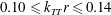
Reference Morison, O’Brien, Johnson and Schaaf1950) with an empirical adjustment of the wave kinematics such as Wheeler stretching incorporated (Wheeler Reference Wheeler1970). As the inertia term in Morison’s formula only includes the force to a first approximation, disregarding possible significant nonlinear contributions (Lighthill Reference Lighthill1979, Reference Lighthill1986), a number of theoretical works have addressed the issue of the high frequency nonlinear loading. Linear- and second-order diffraction solutions capture the first and second harmonic forces in regular and irregular waves, while the solution obtained by Malenica & Molin (Reference Malenica and Molin1995) captures the third harmonic force in regular waves. A long wave approximation (with
 $kr<0.14$
,
$kr<0.14$
,
 $k$
the wavenumber,
$k$
the wavenumber,
 $r$
the cylinder radius, see figure 7) developed by Faltinsen, Newman & Vinje (Reference Faltinsen, Newman and Vinje1995), and referred to as the FNV method, was first obtained for regular waves, and secondly generalized by Newman (Reference Newman, Grue, Gjevik and Weber1996) to the case of irregular waves. Later Krokstad et al. (Reference Krokstad, Stansberg, Nestegård and Marthinsen1998) proposed a modification to the FNV method, where the linear- and second-order contributions were replaced by the complete diffraction solutions. The method was combined with the third-order contribution from the long wave approximation. With an appropriate description of the wave kinematics for realistic wave spectra, Johannessen (Reference Johannessen2010, Reference Johannessen2012) obtained good agreement between the modified FNV method and measurements of a monopile exposed to irregular deep water waves.
$r$
the cylinder radius, see figure 7) developed by Faltinsen, Newman & Vinje (Reference Faltinsen, Newman and Vinje1995), and referred to as the FNV method, was first obtained for regular waves, and secondly generalized by Newman (Reference Newman, Grue, Gjevik and Weber1996) to the case of irregular waves. Later Krokstad et al. (Reference Krokstad, Stansberg, Nestegård and Marthinsen1998) proposed a modification to the FNV method, where the linear- and second-order contributions were replaced by the complete diffraction solutions. The method was combined with the third-order contribution from the long wave approximation. With an appropriate description of the wave kinematics for realistic wave spectra, Johannessen (Reference Johannessen2010, Reference Johannessen2012) obtained good agreement between the modified FNV method and measurements of a monopile exposed to irregular deep water waves.
An alternative nonlinear load description, based on energy considerations, was obtained by Rainey (Reference Rainey1989, Reference Rainey and Eatock Taylor1995a ,Reference Rainey b ). The benefit of the Rainey method is that it takes undisturbed wave kinematics as input. This allows for both nonlinear wave motion and short crestedness to be taken into account. This is in contrast to the FNV method, which is based on the underlying linear wave assumption in a unidirectional sea.
Computational fluid dynamics (CFD) is increasingly being used to calculate the wave loads on offshore structures, see Paulsen, Bredmose & Bingham (Reference Paulsen, Bredmose and Bingham2014a ), Paulsen et al. (Reference Paulsen, Bredmose, Bingham and Jacobsen2014b ). Although CFD is capable of capturing the nonlinearities, the downside is that it is resource demanding. This adds restrictions to the length of analyses with an irregular wave input. Recently, the FNV method has been generalized to a finite water depth by Kristiansen & Faltinsen (Reference Kristiansen and Faltinsen2017).
1.2 Foci of present work
We here investigate the high frequency resonant response of a monopile exposed to irregular waves in deep water, where the short-term statistical variability of the wave conditions is accounted for. The following subjects are included:
(i) We carry out a set of laboratory experiments with a single bottom hinged, rigid cylinder in two different set-ups (§ 2). In the first set-up the cylinder is fixed. The response of an oscillating cylinder is then calculated from the measured wave-exciting moment. The cylinder in the second set-up is free to oscillate where the motion response is measured (§ 3.1).
(ii) In the single wave events of the irregular waves, we identify local proxies such as the local trough-to-trough period and crest height. The higher harmonic load contributions are then investigated by obtaining the third, fourth and fifth harmonic load components in the irregular waves and comparing to published results for regular waves (FNV, Huseby & Grue Reference Huseby and Grue2000; Paulsen et al. Reference Paulsen, Bredmose, Bingham and Jacobsen2014b ) (§ 3.2).
(iii) We identify and investigate several different wave load mechanisms that are present during the large response events (§ 3.3).
(iv) While previous investigations have typically focused on the wave loads acting on the structure only, the present work obtains both the force and the resulting motion. We present the response as a function of resonance frequency, which is varied in the range 3–5 times the peak wave frequency. We obtain the short-term exceedance probability of the response maxima. The linear and nonlinear contributions to the response statistics are compared (§ 3.4).
(v) The most extreme response events are discussed in terms of the local wave slope and non-dimensional trough-to-trough period (§ 3.5).
A conclusion is given in § 4.
2 Experiments
2.1 Wave tank
The experiments were carried out in the wave flume in the hydrodynamic laboratory at the University of Oslo. The wave flume is 25 m long, 0.5 m wide and was filled to a water depth of
 $h=0.72~\text{m}$
. In one end of the tank there is a hydraulic piston-type wavemaker with motion controlled by a preset voltage time series based on linear wavemaker theory. At the opposite end there is a passive absorbing beach. At the location 10.9 m from the wavemaker, a bottom hinged cylinder, with a diameter
$h=0.72~\text{m}$
. In one end of the tank there is a hydraulic piston-type wavemaker with motion controlled by a preset voltage time series based on linear wavemaker theory. At the opposite end there is a passive absorbing beach. At the location 10.9 m from the wavemaker, a bottom hinged cylinder, with a diameter
 $d=6~\text{cm}$
, was placed to obtain the wave-exciting moment and the motion response.
$d=6~\text{cm}$
, was placed to obtain the wave-exciting moment and the motion response.
2.2 Wave conditions
A total of six irregular long-crested wave time series based on the JONSWAP spectrum (Hasselmann et al.
Reference Hasselmann, Barnett, Bouws, Carlson, Cartwright, Enke, Ewing, Gienapp, Hasselmann, Kruseman, Meerburg, Müller, Olbers, Richter, Sell and Walden1973), each 320 s long, were used in the experiments. The JONSWAP spectrum was chosen to generate an approximately real ocean wave environment. The spectrum as a function of angular frequency
 $\unicode[STIX]{x1D714}$
is given by
$\unicode[STIX]{x1D714}$
is given by
 $$\begin{eqnarray}S_{J}(\unicode[STIX]{x1D714}_{n})=A_{\unicode[STIX]{x1D6FE}}\unicode[STIX]{x1D6FC}\unicode[STIX]{x1D714}_{n}^{-5}\exp \left(-{\textstyle \frac{5}{4}}\unicode[STIX]{x1D714}_{n}^{-4}\right)\unicode[STIX]{x1D6FE}^{\exp (-(1/2\unicode[STIX]{x1D70E}^{2})(\unicode[STIX]{x1D714}_{n}-1)^{2})},\end{eqnarray}$$
where
 $\unicode[STIX]{x1D714}_{n}=\unicode[STIX]{x1D714}/\unicode[STIX]{x1D714}_{P}$
and
$\unicode[STIX]{x1D714}_{n}=\unicode[STIX]{x1D714}/\unicode[STIX]{x1D714}_{P}$
and
 $\unicode[STIX]{x1D6FC}=(5/16)\unicode[STIX]{x1D714}_{P}^{-1}H_{S}^{2}$
. The peak wave frequency is denoted by
$\unicode[STIX]{x1D6FC}=(5/16)\unicode[STIX]{x1D714}_{P}^{-1}H_{S}^{2}$
. The peak wave frequency is denoted by
 $\unicode[STIX]{x1D714}_{P}=2\unicode[STIX]{x03C0}/T_{P}$
and the significant wave height by
$\unicode[STIX]{x1D714}_{P}=2\unicode[STIX]{x03C0}/T_{P}$
and the significant wave height by
 $H_{S}=4\unicode[STIX]{x1D70E}_{\unicode[STIX]{x1D702}}$
, where
$H_{S}=4\unicode[STIX]{x1D70E}_{\unicode[STIX]{x1D702}}$
, where
 $T_{P}$
is the peak wave period and
$T_{P}$
is the peak wave period and
 $\unicode[STIX]{x1D70E}_{\unicode[STIX]{x1D702}}$
is the standard deviation of the measured surface elevation. The peak shape parameter is
$\unicode[STIX]{x1D70E}_{\unicode[STIX]{x1D702}}$
is the standard deviation of the measured surface elevation. The peak shape parameter is
 $\unicode[STIX]{x1D6FE}=3.3$
, the spectral width parameter is
$\unicode[STIX]{x1D6FE}=3.3$
, the spectral width parameter is
 $\unicode[STIX]{x1D70E}=0.07$
for
$\unicode[STIX]{x1D70E}=0.07$
for
 $\unicode[STIX]{x1D714}\leqslant \unicode[STIX]{x1D714}_{P}$
and
$\unicode[STIX]{x1D714}\leqslant \unicode[STIX]{x1D714}_{P}$
and
 $\unicode[STIX]{x1D70E}=0.09$
for
$\unicode[STIX]{x1D70E}=0.09$
for
 $\unicode[STIX]{x1D714}>\unicode[STIX]{x1D714}_{P}$
. Further,
$\unicode[STIX]{x1D714}>\unicode[STIX]{x1D714}_{P}$
. Further,
 $A_{\unicode[STIX]{x1D6FE}}=1-0.287\ln (\unicode[STIX]{x1D6FE})$
is a normalization factor.
$A_{\unicode[STIX]{x1D6FE}}=1-0.287\ln (\unicode[STIX]{x1D6FE})$
is a normalization factor.
To relate the wave-exciting moment and motion response to undisturbed wave parameters, the surface elevation was measured with the cylinder removed, using ultra-sound wave sensors (UltraLab ULS Advanced Ultrasound, USS02/HFP with 250 Hz sampling rate). The waves were measured at the location for the cylinder, in addition to 0.12 m and 4.9 m upstream, and 4.4 m downstream.
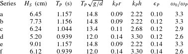
The governing wave parameters of the six time series, given by
 $H_{S}$
and
$H_{S}$
and
 $T_{P}$
at the location of the cylinder, are listed in table 1. Here the peak wavenumber
$T_{P}$
at the location of the cylinder, are listed in table 1. Here the peak wavenumber
 $k_{P}$
is found from the linear dispersion relation
$k_{P}$
is found from the linear dispersion relation
 $\unicode[STIX]{x1D714}_{P}^{2}=gk_{P}\tanh (k_{P}h)$
, where
$\unicode[STIX]{x1D714}_{P}^{2}=gk_{P}\tanh (k_{P}h)$
, where
 $g$
is the acceleration of gravity and
$g$
is the acceleration of gravity and
 $h$
is the water depth. The normalized water depth,
$h$
is the water depth. The normalized water depth,
 $k_{P}h$
, is in the range 2.2–3.3 which is considered to represent deep water waves, and the spectral wave slope,
$k_{P}h$
, is in the range 2.2–3.3 which is considered to represent deep water waves, and the spectral wave slope,
 $\unicode[STIX]{x1D716}_{P}=0.5H_{S}k_{P}$
, is in the range 0.10–0.14 which is considered to represent moderately steep waves. The normalized wavenumber,
$\unicode[STIX]{x1D716}_{P}=0.5H_{S}k_{P}$
, is in the range 0.10–0.14 which is considered to represent moderately steep waves. The normalized wavenumber,
 $k_{P}r$
, where
$k_{P}r$
, where
 $r$
is the radius of the cylinder, is in the range 0.09–0.14 which is considered to be outside of the diffraction regime. The corresponding non-dimensional peak wave period is
$r$
is the radius of the cylinder, is in the range 0.09–0.14 which is considered to be outside of the diffraction regime. The corresponding non-dimensional peak wave period is
 $T_{P}\sqrt{g/d}\sim 12{-}15$
where
$T_{P}\sqrt{g/d}\sim 12{-}15$
where
 $d=2r$
.
$d=2r$
.
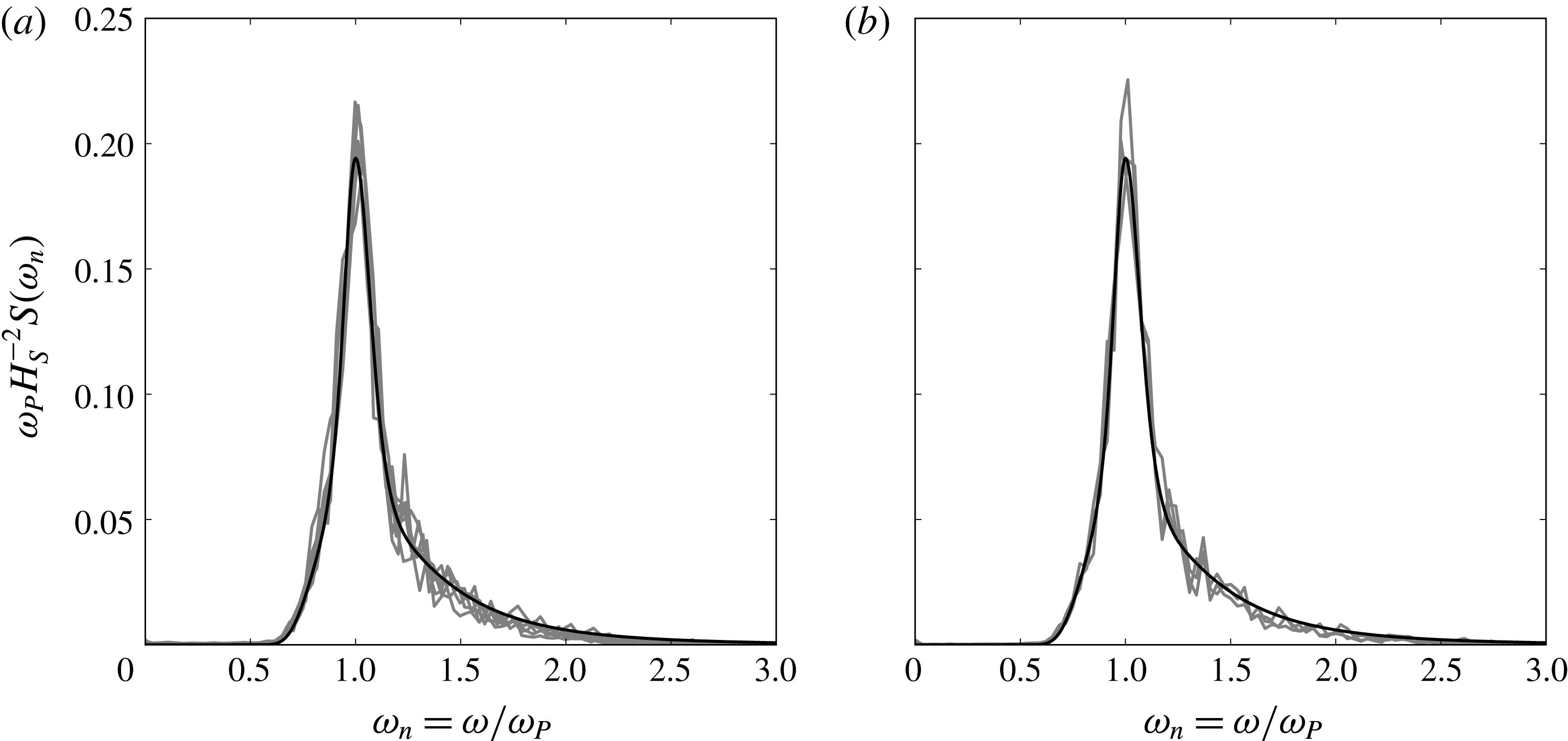
Figure 1. Wave energy density spectrum. Measured surface elevation and JONSWAP spectrum with
 $\unicode[STIX]{x1D6FE}=3.3$
for (a) all of the six time series and (b) time series c, where
$\unicode[STIX]{x1D6FE}=3.3$
for (a) all of the six time series and (b) time series c, where
 $H_{S}=6.24~\text{cm}$
and
$H_{S}=6.24~\text{cm}$
and
 $T_{P}=1.044~\text{s}$
, measured at the location of the cylinder, in addition to 4.9 m upstream and 4.4 m downstream.
$T_{P}=1.044~\text{s}$
, measured at the location of the cylinder, in addition to 4.9 m upstream and 4.4 m downstream.
Table 1. Sea state parameters. Significant wave height
 $H_{S}$
, peak wave period
$H_{S}$
, peak wave period
 $T_{P}$
, normalized peak wave period
$T_{P}$
, normalized peak wave period
 $T_{P}\sqrt{g/d}$
, normalized wavenumber
$T_{P}\sqrt{g/d}$
, normalized wavenumber
 $k_{P}r$
, normalized water depth
$k_{P}r$
, normalized water depth
 $k_{P}h$
, spectral wave slope
$k_{P}h$
, spectral wave slope
 $\unicode[STIX]{x1D716}_{P}=0.5H_{S}k_{P}$
and resonance frequency ratio
$\unicode[STIX]{x1D716}_{P}=0.5H_{S}k_{P}$
and resonance frequency ratio
 $\unicode[STIX]{x1D714}_{0}/\unicode[STIX]{x1D714}_{P}$
as obtained from the oscillating cylinder.
$\unicode[STIX]{x1D714}_{0}/\unicode[STIX]{x1D714}_{P}$
as obtained from the oscillating cylinder.
All of the six measured wave spectra show good agreement with the JONSWAP spectrum, as seen in figure 1(a). In figure 1(b), the spectrum from series c is shown at the cylinder location in addition to 4.9 m upstream and 4.4 m downstream, showing only minor modification in the spectral shape. Between the upstream and downstream locations, the rate of decrease in
 $H_{S}$
is found to be, on average for the six time series, 0.01 per peak wavelength
$H_{S}$
is found to be, on average for the six time series, 0.01 per peak wavelength
 $\unicode[STIX]{x1D706}_{P}=2\unicode[STIX]{x03C0}/k_{P}$
. Measurements from the two wave sensors with a distance of 0.12 m have been used to estimate the reflection from the beach. For the governing wave frequencies,
$\unicode[STIX]{x1D706}_{P}=2\unicode[STIX]{x03C0}/k_{P}$
. Measurements from the two wave sensors with a distance of 0.12 m have been used to estimate the reflection from the beach. For the governing wave frequencies,
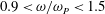 $0.9<\unicode[STIX]{x1D714}/\unicode[STIX]{x1D714}_{P}<1.5$
, the reflection coefficient, in terms of the amplitude, as outlined by Goda & Suzuki (Reference Goda and Suzuki1976), is found to be less than 0.06.
$0.9<\unicode[STIX]{x1D714}/\unicode[STIX]{x1D714}_{P}<1.5$
, the reflection coefficient, in terms of the amplitude, as outlined by Goda & Suzuki (Reference Goda and Suzuki1976), is found to be less than 0.06.
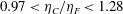
2.3 Local wave properties and statistics
The surface elevation at a fixed position in the wave tank is a function of time. It is convenient to define a single wave event by its crest elevation,
 $\unicode[STIX]{x1D702}_{C}$
, and its trough-to-trough period,
$\unicode[STIX]{x1D702}_{C}$
, and its trough-to-trough period,
 $T_{TT}$
, see figure 2(a). Altogether, the six time series consist of in total 2166 single wave events. A scatter plot of
$T_{TT}$
, see figure 2(a). Altogether, the six time series consist of in total 2166 single wave events. A scatter plot of
 $\unicode[STIX]{x1D702}_{C}$
and
$\unicode[STIX]{x1D702}_{C}$
and
 $T_{TT}$
, measured at the location of the cylinder, is shown in figure 2(b).
$T_{TT}$
, measured at the location of the cylinder, is shown in figure 2(b).
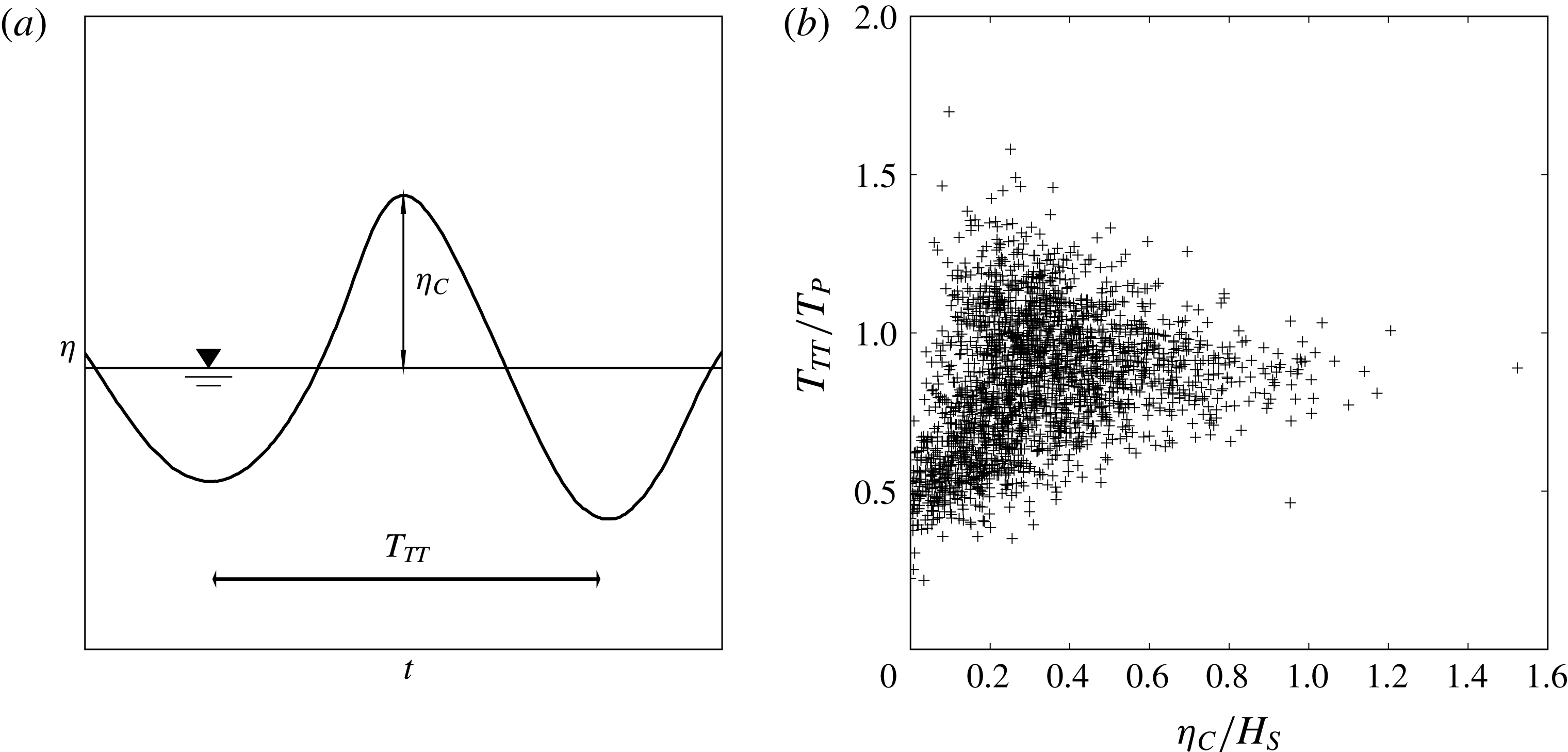
Figure 2. Local wave properties. (a) Definition of crest height
 $\unicode[STIX]{x1D702}_{C}$
and trough-to-trough wave period
$\unicode[STIX]{x1D702}_{C}$
and trough-to-trough wave period
 $T_{TT}$
of a wave event and (b) wave scatter plot including all of the 2166 measured waves (
$T_{TT}$
of a wave event and (b) wave scatter plot including all of the 2166 measured waves (
 $+$
).
$+$
).
For a group of events the empirical probability of exceedance is given by
 $$\begin{eqnarray}P_{ex}(x_{i})=1-P(X\leqslant x_{i})=1-\text{i}/(N+1),\end{eqnarray}$$
where
 $x_{i}$
for
$x_{i}$
for
 $\text{i}=1,2,\ldots ,N$
indicates the events in ascending order, and
$\text{i}=1,2,\ldots ,N$
indicates the events in ascending order, and
 $N$
is the total number of the events. In figure 3(a) the crest height exceedance probability
$N$
is the total number of the events. In figure 3(a) the crest height exceedance probability
 $P_{ex}(\unicode[STIX]{x1D702}_{C}/Hs)$
, as found from series c, is presented and compared to the linear Rayleigh and the second-order Forristall crest distribution (Forristall Reference Forristall2000). It is observed that the measurements contain somewhat larger crest heights than expected based on the second-order distribution. This is further visualized by comparing the largest crest elevations from all of the series with the corresponding Forristall distribution. If
$P_{ex}(\unicode[STIX]{x1D702}_{C}/Hs)$
, as found from series c, is presented and compared to the linear Rayleigh and the second-order Forristall crest distribution (Forristall Reference Forristall2000). It is observed that the measurements contain somewhat larger crest heights than expected based on the second-order distribution. This is further visualized by comparing the largest crest elevations from all of the series with the corresponding Forristall distribution. If
 $\unicode[STIX]{x1D702}_{F}$
denotes the Forristall crest height estimate, the largest crest height observed with regards to significant wave height,
$\unicode[STIX]{x1D702}_{F}$
denotes the Forristall crest height estimate, the largest crest height observed with regards to significant wave height,
 $\unicode[STIX]{x1D702}_{C}/H_{S}=1.5$
, has
$\unicode[STIX]{x1D702}_{C}/H_{S}=1.5$
, has
 $\unicode[STIX]{x1D702}_{C}/\unicode[STIX]{x1D702}_{F}=1.6$
(found in series d and seen in figure 2
b). Except for this extreme crest event, a plot of
$\unicode[STIX]{x1D702}_{C}/\unicode[STIX]{x1D702}_{F}=1.6$
(found in series d and seen in figure 2
b). Except for this extreme crest event, a plot of
 $\unicode[STIX]{x1D702}_{C}/\unicode[STIX]{x1D702}_{F}$
versus its probability shows
$\unicode[STIX]{x1D702}_{C}/\unicode[STIX]{x1D702}_{F}$
versus its probability shows
 $0.97<\unicode[STIX]{x1D702}_{C}/\unicode[STIX]{x1D702}_{F}<1.28$
for the 10 % largest waves, for all of the six series, see figure 3(b).
$0.97<\unicode[STIX]{x1D702}_{C}/\unicode[STIX]{x1D702}_{F}<1.28$
for the 10 % largest waves, for all of the six series, see figure 3(b).

Figure 3. Crest height exceedance probability for (a) series c,
 $H_{S}=6.24~\text{cm}$
and
$H_{S}=6.24~\text{cm}$
and
 $T_{P}=1.044~\text{s}$
(
$T_{P}=1.044~\text{s}$
(
 $+$
), linear Rayleigh (– –) and second-order Forristall (——) and (b) measured crest heights, normalized with the corresponding Forristall estimate, the 10 % largest crest heights from each series, series a (▵), b (▫), c (
$+$
), linear Rayleigh (– –) and second-order Forristall (——) and (b) measured crest heights, normalized with the corresponding Forristall estimate, the 10 % largest crest heights from each series, series a (▵), b (▫), c (
 $+$
), d (♢), e (
$+$
), d (♢), e (
 $\times$
) and f (○).
$\times$
) and f (○).
For later purposes (§§ 3.2 and 3.5), and following Grue et al. (Reference Grue, Clamond, Huseby and Jensen2003), using a variant of the Stokes’ third-order approximation, the measured
 $\unicode[STIX]{x1D702}_{C}$
and
$\unicode[STIX]{x1D702}_{C}$
and
 $T_{TT}$
are used to define a local wavenumber,
$T_{TT}$
are used to define a local wavenumber,
 $k_{TT}$
, and local wave slope,
$k_{TT}$
, and local wave slope,
 $\unicode[STIX]{x1D716}$
, of the event by
$\unicode[STIX]{x1D716}$
, of the event by
 $$\begin{eqnarray}\unicode[STIX]{x1D714}_{TT}^{2}=gk_{TT}(1+\unicode[STIX]{x1D716}^{2})\quad \text{and}\quad k_{TT}\unicode[STIX]{x1D702}_{C}=\unicode[STIX]{x1D716}+{\textstyle \frac{1}{2}}\unicode[STIX]{x1D716}^{2}+{\textstyle \frac{1}{2}}\unicode[STIX]{x1D716}^{3},\end{eqnarray}$$
where
 $\unicode[STIX]{x1D714}_{TT}=2\unicode[STIX]{x03C0}/T_{TT}$
,
$\unicode[STIX]{x1D714}_{TT}=2\unicode[STIX]{x03C0}/T_{TT}$
,
 $\unicode[STIX]{x1D716}=ak_{TT}$
and
$\unicode[STIX]{x1D716}=ak_{TT}$
and
 $a$
is the approximated underlying linear amplitude. This enables a wave parametrization of each of the single wave events in the irregular wave time series. From the same approach a maximum horizontal particle velocity below the crest is estimated by
$a$
is the approximated underlying linear amplitude. This enables a wave parametrization of each of the single wave events in the irregular wave time series. From the same approach a maximum horizontal particle velocity below the crest is estimated by
 $u_{C}=\unicode[STIX]{x1D716}\sqrt{g/k_{TT}}\exp (k_{TT}\unicode[STIX]{x1D702}_{C})$
. The estimation of
$u_{C}=\unicode[STIX]{x1D716}\sqrt{g/k_{TT}}\exp (k_{TT}\unicode[STIX]{x1D702}_{C})$
. The estimation of
 $\unicode[STIX]{x1D716}$
,
$\unicode[STIX]{x1D716}$
,
 $k_{TT}$
and
$k_{TT}$
and
 $u_{C}$
in irregular waves have been further tested by Stansberg, Gudmestad & Haver (Reference Stansberg, Gudmestad and Haver2008) and Grue & Jensen (Reference Grue and Jensen2012), showing good agreement with experimental results.
$u_{C}$
in irregular waves have been further tested by Stansberg, Gudmestad & Haver (Reference Stansberg, Gudmestad and Haver2008) and Grue & Jensen (Reference Grue and Jensen2012), showing good agreement with experimental results.
2.4 Cylinder model
A single cylinder with diameter
 $d=6~\text{cm}$
, in two different set-ups, was used in the experiments. The cylinder was located 10.9 m from the wavemaker and hinged at a horizontal lateral axis at the level of
$d=6~\text{cm}$
, in two different set-ups, was used in the experiments. The cylinder was located 10.9 m from the wavemaker and hinged at a horizontal lateral axis at the level of
 $z=z_{0}=2~\text{cm}$
above the tank bottom, with positive rotation in the wave propagation direction. At a distance of
$z=z_{0}=2~\text{cm}$
above the tank bottom, with positive rotation in the wave propagation direction. At a distance of
 $z_{a}-z_{0}=90~\text{cm}$
above the rotation axis, the cylinder was connected to two load cells (Hottinger Baldwin Messtechnik Type Z6C2 with
$z_{a}-z_{0}=90~\text{cm}$
above the rotation axis, the cylinder was connected to two load cells (Hottinger Baldwin Messtechnik Type Z6C2 with
 $10~\text{kg}=2~\text{mV}~\text{V}^{-1}$
and 400 Hz sampling rate), measuring the force from which the overturning moment was determined. In the first set-up the cylinder was fixed and rigidly connected to the load cells, where the wave-exciting force and moment with respect to
$10~\text{kg}=2~\text{mV}~\text{V}^{-1}$
and 400 Hz sampling rate), measuring the force from which the overturning moment was determined. In the first set-up the cylinder was fixed and rigidly connected to the load cells, where the wave-exciting force and moment with respect to
 $z_{0}$
are measured. In the second set-up the cylinder was free to oscillate and springs were used to connect the model and the load cells.
$z_{0}$
are measured. In the second set-up the cylinder was free to oscillate and springs were used to connect the model and the load cells.

Figure 4. Oscillating cylinder set-up with angular rotation
 $\unicode[STIX]{x1D703}(t)$
, cylinder diameter
$\unicode[STIX]{x1D703}(t)$
, cylinder diameter
 $D=0.06~\text{m}$
, water depth
$D=0.06~\text{m}$
, water depth
 $h=0.72~\text{m}$
, rotation point
$h=0.72~\text{m}$
, rotation point
 $z_{0}=0.02~\text{m}$
, distance from tank bottom to load cells
$z_{0}=0.02~\text{m}$
, distance from tank bottom to load cells
 $z_{a}=0.92~\text{m}$
, load cells
$z_{a}=0.92~\text{m}$
, load cells
 $F_{1}$
and
$F_{1}$
and
 $F_{2}$
, distance to wavemaker
$F_{2}$
, distance to wavemaker
 $L_{WM}=10.90~\text{m}$
and distance to tank end,
$L_{WM}=10.90~\text{m}$
and distance to tank end,
 $L_{TE}=13.87~\text{m}$
.
$L_{TE}=13.87~\text{m}$
.
A sketch of the second set-up is shown in figure 4. The vertical cylinder is free to rotate with an angle
 $\unicode[STIX]{x1D703}(t)$
in the pitch mode of motion. Assuming linear motion, the moment due to the pressure forces with respect to
$\unicode[STIX]{x1D703}(t)$
in the pitch mode of motion. Assuming linear motion, the moment due to the pressure forces with respect to
 $z_{0}$
reads:
$z_{0}$
reads:
 $M_{wave}(t)-a_{55}\ddot{\unicode[STIX]{x1D703}}-b_{55}\dot{\unicode[STIX]{x1D703}}-c_{55}\unicode[STIX]{x1D703}$
, where
$M_{wave}(t)-a_{55}\ddot{\unicode[STIX]{x1D703}}-b_{55}\dot{\unicode[STIX]{x1D703}}-c_{55}\unicode[STIX]{x1D703}$
, where
 $M_{wave}(t)$
,
$M_{wave}(t)$
,
 $a_{55}$
,
$a_{55}$
,
 $b_{55}$
and
$b_{55}$
and
 $c_{55}$
denote the wave-exciting moment obtained from the fixed cylinder set-up, added mass, damping and restoring coefficients in the pitch mode of motion, respectively. The moment due to the spring forces reads:
$c_{55}$
denote the wave-exciting moment obtained from the fixed cylinder set-up, added mass, damping and restoring coefficients in the pitch mode of motion, respectively. The moment due to the spring forces reads:
 $-(z_{a}-z_{0})(F_{2}(t)-F_{1}(t))=-\unicode[STIX]{x1D705}_{0}(z_{a}-z_{0})^{2}\unicode[STIX]{x1D703}$
where
$-(z_{a}-z_{0})(F_{2}(t)-F_{1}(t))=-\unicode[STIX]{x1D705}_{0}(z_{a}-z_{0})^{2}\unicode[STIX]{x1D703}$
where
 $F_{1}$
and
$F_{1}$
and
 $F_{2}$
denote the force recorded at the left and right transducer, respectively, see figure 4, and
$F_{2}$
denote the force recorded at the left and right transducer, respectively, see figure 4, and
 $\unicode[STIX]{x1D705}_{0}$
the spring constant. Balance of angular momentum gives
$\unicode[STIX]{x1D705}_{0}$
the spring constant. Balance of angular momentum gives
 $$\begin{eqnarray}m_{55}\ddot{\unicode[STIX]{x1D703}}=-a_{55}\ddot{\unicode[STIX]{x1D703}}-b_{55}\dot{\unicode[STIX]{x1D703}}-(\unicode[STIX]{x1D705}_{0}(z_{a}-z_{0})^{2}+c_{55})\unicode[STIX]{x1D703}+M_{wave}(t),\end{eqnarray}$$
where
 $m_{55}$
denotes the moment of inertia of the cylinder.
$m_{55}$
denotes the moment of inertia of the cylinder.
The resonance frequency of (2.4) is given by
 $\unicode[STIX]{x1D714}_{0}^{2}=(c_{55}+\unicode[STIX]{x1D705}_{0}(z_{a}-z_{0})^{2})/(m_{55}+a_{55})$
. Note that the spring force provides the dominant contribution to the restoring force where
$\unicode[STIX]{x1D714}_{0}^{2}=(c_{55}+\unicode[STIX]{x1D705}_{0}(z_{a}-z_{0})^{2})/(m_{55}+a_{55})$
. Note that the spring force provides the dominant contribution to the restoring force where
 $c_{55}$
is 0.005 times
$c_{55}$
is 0.005 times
 $\unicode[STIX]{x1D705}_{0}(z_{a}-z_{0})^{2}$
for the actual cylinder. The still water decay tests as well as the irregular wave experiments determine
$\unicode[STIX]{x1D705}_{0}(z_{a}-z_{0})^{2}$
for the actual cylinder. The still water decay tests as well as the irregular wave experiments determine
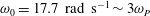 $\unicode[STIX]{x1D714}_{0}=17.7~\text{rad}~\text{s}^{-1}\sim 3\unicode[STIX]{x1D714}_{P}$
(table 1) of the oscillating cylinder. The damping ratio
$\unicode[STIX]{x1D714}_{0}=17.7~\text{rad}~\text{s}^{-1}\sim 3\unicode[STIX]{x1D714}_{P}$
(table 1) of the oscillating cylinder. The damping ratio
 $\unicode[STIX]{x1D701}$
, determined as a fraction of the critical damping, is 0.02 for the cylinder. The small damping ratio implies a very lightly damped oscillating system relevant to offshore wind turbines in extreme conditions (Kallehave et al.
Reference Kallehave, Byrne, Thilsted and Mikkelsen2015).
$\unicode[STIX]{x1D701}$
, determined as a fraction of the critical damping, is 0.02 for the cylinder. The small damping ratio implies a very lightly damped oscillating system relevant to offshore wind turbines in extreme conditions (Kallehave et al.
Reference Kallehave, Byrne, Thilsted and Mikkelsen2015).
By integration, the pitch angle
 $\unicode[STIX]{x1D703}(t)$
is obtained as a function of time. For convenience, the response is multiplied by
$\unicode[STIX]{x1D703}(t)$
is obtained as a function of time. For convenience, the response is multiplied by
 $\unicode[STIX]{x1D705}_{0}(z_{a}-z_{0})^{2}$
, giving the moment of the sum spring force with respect to
$\unicode[STIX]{x1D705}_{0}(z_{a}-z_{0})^{2}$
, giving the moment of the sum spring force with respect to
 $z_{0}$
. We denote this quantity by
$z_{0}$
. We denote this quantity by
 $R(\unicode[STIX]{x1D714}_{0},t)$
where
$R(\unicode[STIX]{x1D714}_{0},t)$
where
 $$\begin{eqnarray}R(\unicode[STIX]{x1D714}_{0},t)=\unicode[STIX]{x1D705}_{0}(z_{a}-z_{0})^{2}\unicode[STIX]{x1D703}(t)=\frac{\unicode[STIX]{x1D714}_{0}^{2}}{\unicode[STIX]{x1D714}_{d}}\int _{0}^{t}M_{wave}(\unicode[STIX]{x1D70F})\text{e}^{-\unicode[STIX]{x1D701}\unicode[STIX]{x1D714}_{0}(t-\unicode[STIX]{x1D70F})}\sin (\unicode[STIX]{x1D714}_{d}(t-\unicode[STIX]{x1D70F}))\,\text{d}\unicode[STIX]{x1D70F},\end{eqnarray}$$
and
 $\unicode[STIX]{x1D714}_{d}=\unicode[STIX]{x1D714}_{0}\sqrt{1-\unicode[STIX]{x1D701}^{2}}$
. A derivation of (2.5), commonly known as Duhamel’s integral, is given in appendix A. Using (2.5) to obtain the motion response
$\unicode[STIX]{x1D714}_{d}=\unicode[STIX]{x1D714}_{0}\sqrt{1-\unicode[STIX]{x1D701}^{2}}$
. A derivation of (2.5), commonly known as Duhamel’s integral, is given in appendix A. Using (2.5) to obtain the motion response
 $R(\unicode[STIX]{x1D714}_{0},t)$
, this is fully described by the wave-exciting moment, the resonance frequency and the damping ratio. Use of (2.5) makes possible a response analysis given
$R(\unicode[STIX]{x1D714}_{0},t)$
, this is fully described by the wave-exciting moment, the resonance frequency and the damping ratio. Use of (2.5) makes possible a response analysis given
 $M_{wave}(t)$
on the fixed cylinder and varying the resonance frequency
$M_{wave}(t)$
on the fixed cylinder and varying the resonance frequency
 $\unicode[STIX]{x1D714}_{0}$
to investigate the response dependency on the ratio
$\unicode[STIX]{x1D714}_{0}$
to investigate the response dependency on the ratio
 $\unicode[STIX]{x1D714}_{0}/\unicode[STIX]{x1D714}_{P}$
. We shall find a good correspondence between the measured and calculated response maxima, see § 3.1.
$\unicode[STIX]{x1D714}_{0}/\unicode[STIX]{x1D714}_{P}$
. We shall find a good correspondence between the measured and calculated response maxima, see § 3.1.
For the calculations of the response, a low pass filter has been applied above the significant wave frequencies at the frequency
 $\unicode[STIX]{x1D714}=60~\text{rad}~\text{s}^{-1}>9\unicode[STIX]{x1D714}_{P}$
. This is considered as well above the significant wave and load frequencies of interest.
$\unicode[STIX]{x1D714}=60~\text{rad}~\text{s}^{-1}>9\unicode[STIX]{x1D714}_{P}$
. This is considered as well above the significant wave and load frequencies of interest.
3 Wave loads and responses
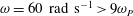
Figure 5. Series c (
 $t=155.7~\text{s}$
),
$t=155.7~\text{s}$
),
 $H_{S}=6.24~\text{cm}$
,
$H_{S}=6.24~\text{cm}$
,
 $T_{P}=1.044~\text{s}$
. (a) Surface elevation, (b) wave-exciting moment, (c) higher harmonic wave force components,
$T_{P}=1.044~\text{s}$
. (a) Surface elevation, (b) wave-exciting moment, (c) higher harmonic wave force components,
 $(h-z_{0})F^{(3\unicode[STIX]{x1D714}_{TT})}$
(- - -),
$(h-z_{0})F^{(3\unicode[STIX]{x1D714}_{TT})}$
(- - -),
 $(h-z_{0})F^{(4\unicode[STIX]{x1D714}_{TT})}$
(– –),
$(h-z_{0})F^{(4\unicode[STIX]{x1D714}_{TT})}$
(– –),
 $(h-z_{0})F^{(5\unicode[STIX]{x1D714}_{TT})}$
(——), (d) measured (——) and calculated (– –) response for
$(h-z_{0})F^{(5\unicode[STIX]{x1D714}_{TT})}$
(——), (d) measured (——) and calculated (– –) response for
 $\unicode[STIX]{x1D714}_{0}/\unicode[STIX]{x1D714}_{P}=2.9$
, (e) measured (——) and calculated (– –) dynamic contribution for
$\unicode[STIX]{x1D714}_{0}/\unicode[STIX]{x1D714}_{P}=2.9$
, (e) measured (——) and calculated (– –) dynamic contribution for
 $\unicode[STIX]{x1D714}_{0}/\unicode[STIX]{x1D714}_{P}=2.9$
, (f) calculated response (——) and measured wave-exciting moment (– –) for
$\unicode[STIX]{x1D714}_{0}/\unicode[STIX]{x1D714}_{P}=2.9$
, (f) calculated response (——) and measured wave-exciting moment (– –) for
 $\unicode[STIX]{x1D714}_{0}/\unicode[STIX]{x1D714}_{P}=2.0$
and (g) calculated response (——) and measured wave-exciting moment (– –) for
$\unicode[STIX]{x1D714}_{0}/\unicode[STIX]{x1D714}_{P}=2.0$
and (g) calculated response (——) and measured wave-exciting moment (– –) for
 $\unicode[STIX]{x1D714}_{0}/\unicode[STIX]{x1D714}_{P}=4.0$
.
$\unicode[STIX]{x1D714}_{0}/\unicode[STIX]{x1D714}_{P}=4.0$
.
The surface elevation, wave-exciting moment and motion response for a large event, occurring between two subsequent zero up-crossings of the moment history, are shown in figure 5. The various plots in the figure illustrate different effects observed in the run; these different effects are discussed in §§ 3.1–3.3. The zero up-crossing period of the moment,
 $T_{z0}^{M}$
, is illustrated in figure 5(b). The periods
$T_{z0}^{M}$
, is illustrated in figure 5(b). The periods
 $T_{TT}$
and
$T_{TT}$
and
 $T_{z0}^{M}$
occur approximately in the same time window, but they are not exactly equal. The period
$T_{z0}^{M}$
occur approximately in the same time window, but they are not exactly equal. The period
 $T_{TT}$
is used in combination with the measured wave elevation to define the wave proxies,
$T_{TT}$
is used in combination with the measured wave elevation to define the wave proxies,
 $\unicode[STIX]{x1D716}$
and
$\unicode[STIX]{x1D716}$
and
 $k_{TT}$
in (2.3), for presentation of the higher harmonic forces in § 3.2 and the extreme response events in §§ 3.3 and 3.5. The
$k_{TT}$
in (2.3), for presentation of the higher harmonic forces in § 3.2 and the extreme response events in §§ 3.3 and 3.5. The
 $T_{z0}^{M}$
is used in combination with the wave-exciting moment time series giving the load and response statistics, using (2.2), with results presented in §§ 3.1 and 3.4.
$T_{z0}^{M}$
is used in combination with the wave-exciting moment time series giving the load and response statistics, using (2.2), with results presented in §§ 3.1 and 3.4.
The wave event occurs in time series c where
 $T_{P}=1.044~\text{s}$
and
$T_{P}=1.044~\text{s}$
and
 $\unicode[STIX]{x1D714}_{P}=2\unicode[STIX]{x03C0}/T_{P}$
, giving a frequency ratio of
$\unicode[STIX]{x1D714}_{P}=2\unicode[STIX]{x03C0}/T_{P}$
, giving a frequency ratio of
 $\unicode[STIX]{x1D714}_{0}/\unicode[STIX]{x1D714}_{P}=2.9$
where
$\unicode[STIX]{x1D714}_{0}/\unicode[STIX]{x1D714}_{P}=2.9$
where
 $\unicode[STIX]{x1D714}_{0}=17.7~\text{rad}~\text{s}^{-1}$
. The surface elevation in figure 5(a) is normalized by the significant wave height
$\unicode[STIX]{x1D714}_{0}=17.7~\text{rad}~\text{s}^{-1}$
. The surface elevation in figure 5(a) is normalized by the significant wave height
 $H_{S}$
, and the load and responses in figure 5(b–g) are normalized by the standard deviation of the wave-exciting moment,
$H_{S}$
, and the load and responses in figure 5(b–g) are normalized by the standard deviation of the wave-exciting moment,
 $\unicode[STIX]{x1D70E}_{M}$
. Three repetitions of the time series are included in the figure and we note that the repeatability is good with only very small differences at the wave crest.
$\unicode[STIX]{x1D70E}_{M}$
. Three repetitions of the time series are included in the figure and we note that the repeatability is good with only very small differences at the wave crest.
The different types of high frequency response may be categorized either as springing or ringing. In figures 5(f) and 5(g) calculations have been carried out for two different resonance frequencies, of
 $\unicode[STIX]{x1D714}_{0}/\unicode[STIX]{x1D714}_{P}=2$
and
$\unicode[STIX]{x1D714}_{0}/\unicode[STIX]{x1D714}_{P}=2$
and
 $\unicode[STIX]{x1D714}_{0}/\unicode[STIX]{x1D714}_{P}=4$
, respectively, using the measured wave-exciting moment and the transfer function. The results illustrate a response of the springing type (
$\unicode[STIX]{x1D714}_{0}/\unicode[STIX]{x1D714}_{P}=4$
, respectively, using the measured wave-exciting moment and the transfer function. The results illustrate a response of the springing type (
 $\unicode[STIX]{x1D714}_{0}/\unicode[STIX]{x1D714}_{P}=2$
) and of the ringing type (
$\unicode[STIX]{x1D714}_{0}/\unicode[STIX]{x1D714}_{P}=2$
) and of the ringing type (
 $\unicode[STIX]{x1D714}_{0}/\unicode[STIX]{x1D714}_{P}=4$
). The springing behaviour is global in time, while ringing is local in time.
$\unicode[STIX]{x1D714}_{0}/\unicode[STIX]{x1D714}_{P}=4$
). The springing behaviour is global in time, while ringing is local in time.
3.1 Single response maxima
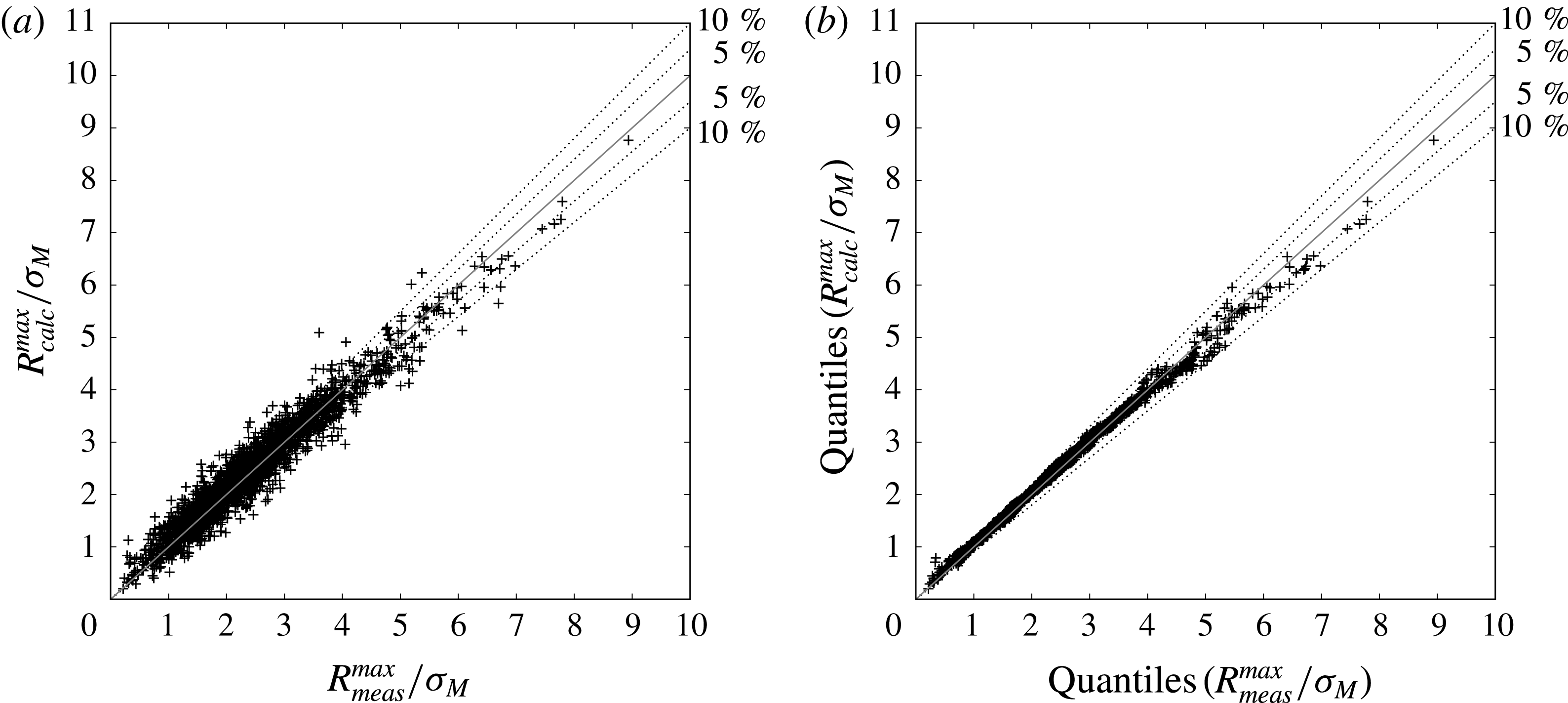
Figure 6. All of the six time series with 2166 events (
 $+$
) where
$+$
) where
 $2.6<\unicode[STIX]{x1D714}_{0}/\unicode[STIX]{x1D714}_{P}<3.3$
. Comparing response maxima by (a) direct comparison and (b) quantiles (sorted values).
$2.6<\unicode[STIX]{x1D714}_{0}/\unicode[STIX]{x1D714}_{P}<3.3$
. Comparing response maxima by (a) direct comparison and (b) quantiles (sorted values).
The response maxima, obtained from the measured wave-exciting moment on the fixed cylinder, with the resonance calculated by the transfer function (2.5), denoted by
 $R_{calc}^{max}=\max (R(\unicode[STIX]{x1D714}_{0},t))$
, are compared to the measured response, denoted by
$R_{calc}^{max}=\max (R(\unicode[STIX]{x1D714}_{0},t))$
, are compared to the measured response, denoted by
 $R_{meas}^{max}$
. The data from all of the six time series give a total of 2166 events with a frequency ratio in the range
$R_{meas}^{max}$
. The data from all of the six time series give a total of 2166 events with a frequency ratio in the range
 $2.6<\unicode[STIX]{x1D714}_{0}/\unicode[STIX]{x1D714}_{P}<3.3$
. The two quantities show good agreement for the largest response events
$2.6<\unicode[STIX]{x1D714}_{0}/\unicode[STIX]{x1D714}_{P}<3.3$
. The two quantities show good agreement for the largest response events
 $R_{meas}^{max}/\unicode[STIX]{x1D70E}_{M}>7$
, where the deviation is up to approximately 5 %, see figure 6(a). Good agreement is also found when looking at the calculated and measured maxima, sorted according to magnitude, denoted by the so-called quantiles, see figure 6(b). This justifies the use of the measured wave-exciting moment in combination with the transfer function, both for estimating the probability levels and for the identification of the extreme events. In what follows, we obtain only the calculated response maxima using the notation
$R_{meas}^{max}/\unicode[STIX]{x1D70E}_{M}>7$
, where the deviation is up to approximately 5 %, see figure 6(a). Good agreement is also found when looking at the calculated and measured maxima, sorted according to magnitude, denoted by the so-called quantiles, see figure 6(b). This justifies the use of the measured wave-exciting moment in combination with the transfer function, both for estimating the probability levels and for the identification of the extreme events. In what follows, we obtain only the calculated response maxima using the notation
 $R^{max}=R_{calc}^{max}$
, for the extended frequency range
$R^{max}=R_{calc}^{max}$
, for the extended frequency range
 $\unicode[STIX]{x1D714}_{0}/\unicode[STIX]{x1D714}_{P}=3,4$
and 5.
$\unicode[STIX]{x1D714}_{0}/\unicode[STIX]{x1D714}_{P}=3,4$
and 5.
3.2 Higher harmonic wave forces
The high frequency response is driven by higher harmonic wave force components. We investigate the third, fourth and fifth harmonic forces with regards to the local wave period
 $T_{TT}$
. The forces are obtained from the wave-exciting moment assuming that they are acting at the still water level. The high frequency forces are considered to act close to the surface (Rainey Reference Rainey1989, Reference Rainey and Eatock Taylor1995a
,Reference Rainey
b
; Faltinsen et al.
Reference Faltinsen, Newman and Vinje1995; Newman Reference Newman, Grue, Gjevik and Weber1996), which indicates an error of less than
$T_{TT}$
. The forces are obtained from the wave-exciting moment assuming that they are acting at the still water level. The high frequency forces are considered to act close to the surface (Rainey Reference Rainey1989, Reference Rainey and Eatock Taylor1995a
,Reference Rainey
b
; Faltinsen et al.
Reference Faltinsen, Newman and Vinje1995; Newman Reference Newman, Grue, Gjevik and Weber1996), which indicates an error of less than
 $(\unicode[STIX]{x1D702}_{C}/h)$
when using the moment to obtain the forces. For each of the single events, where an event is defined in figure 5(a,b), a window function of 20 s has been applied, from which the high frequency harmonic force components are extracted, see figure 5(c). The maximum amplitude found within the event is defined as the local high frequency harmonic force contribution.
$(\unicode[STIX]{x1D702}_{C}/h)$
when using the moment to obtain the forces. For each of the single events, where an event is defined in figure 5(a,b), a window function of 20 s has been applied, from which the high frequency harmonic force components are extracted, see figure 5(c). The maximum amplitude found within the event is defined as the local high frequency harmonic force contribution.
The third harmonic force
 $F^{(3\unicode[STIX]{x1D714}_{TT})}$
is found using a filter covering
$F^{(3\unicode[STIX]{x1D714}_{TT})}$
is found using a filter covering
 $2.5<\unicode[STIX]{x1D714}/\unicode[STIX]{x1D714}_{TT}<3.5$
. Likewise, the fourth harmonic force
$2.5<\unicode[STIX]{x1D714}/\unicode[STIX]{x1D714}_{TT}<3.5$
. Likewise, the fourth harmonic force
 $F^{(4\unicode[STIX]{x1D714}_{TT})}$
is found for
$F^{(4\unicode[STIX]{x1D714}_{TT})}$
is found for
 $3.5<\unicode[STIX]{x1D714}/\unicode[STIX]{x1D714}_{TT}<4.5$
, and the fifth harmonic force
$3.5<\unicode[STIX]{x1D714}/\unicode[STIX]{x1D714}_{TT}<4.5$
, and the fifth harmonic force
 $F^{(5\unicode[STIX]{x1D714}_{TT})}$
using
$F^{(5\unicode[STIX]{x1D714}_{TT})}$
using
 $4.5<\unicode[STIX]{x1D714}/\unicode[STIX]{x1D714}_{TT}<5.5$
. The forces are expressed for the proxies; the normalized wavenumber
$4.5<\unicode[STIX]{x1D714}/\unicode[STIX]{x1D714}_{TT}<5.5$
. The forces are expressed for the proxies; the normalized wavenumber
 $k_{TT}r$
and the wave slope
$k_{TT}r$
and the wave slope
 $\unicode[STIX]{x1D716}=ak_{TT}$
, where both are defined in (2.3) and
$\unicode[STIX]{x1D716}=ak_{TT}$
, where both are defined in (2.3) and
 $r$
is the cylinder radius. The obtained results from the irregular waves are compared to previous works with a regular wave input; the leading-order third harmonic FNV solution,
$r$
is the cylinder radius. The obtained results from the irregular waves are compared to previous works with a regular wave input; the leading-order third harmonic FNV solution,
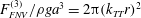 $F_{FNV}^{(3)}/\unicode[STIX]{x1D70C}ga^{3}=2\unicode[STIX]{x03C0}(k_{TT}r)^{2}$
, the measurements from Huseby & Grue (Reference Huseby and Grue2000), denoted by H&G and the CFD computations for finite depth by Paulsen et al. (Reference Paulsen, Bredmose, Bingham and Jacobsen2014b
).
$F_{FNV}^{(3)}/\unicode[STIX]{x1D70C}ga^{3}=2\unicode[STIX]{x03C0}(k_{TT}r)^{2}$
, the measurements from Huseby & Grue (Reference Huseby and Grue2000), denoted by H&G and the CFD computations for finite depth by Paulsen et al. (Reference Paulsen, Bredmose, Bingham and Jacobsen2014b
).
For the longest waves, with
 $0.10\leqslant k_{TT}r\leqslant 0.14$
(
$0.10\leqslant k_{TT}r\leqslant 0.14$
(
 $14.1>T_{TT}^{0}\sqrt{g/d}>11.9$
, where
$14.1>T_{TT}^{0}\sqrt{g/d}>11.9$
, where
 $T_{TT}^{0}$
is the linear estimate) we observe that
$T_{TT}^{0}$
is the linear estimate) we observe that
 $F^{(3\unicode[STIX]{x1D714}_{TT})}$
tends towards a constant level close to the FNV result, with the average of the irregular results approximately 11 % below the theory (figure 7
a). The FNV force is evaluated for the middle value of
$F^{(3\unicode[STIX]{x1D714}_{TT})}$
tends towards a constant level close to the FNV result, with the average of the irregular results approximately 11 % below the theory (figure 7
a). The FNV force is evaluated for the middle value of
 $k_{TT}r$
in each of the
$k_{TT}r$
in each of the
 $k_{TT}r$
ranges. In the range
$k_{TT}r$
ranges. In the range
 $0.14\leqslant k_{TT}r\leqslant 0.18$
(
$0.14\leqslant k_{TT}r\leqslant 0.18$
(
 $11.9>T_{TT}^{0}\sqrt{g/d}>10.5$
), the results from H&G are lower, but within the standard deviation of the present irregular wave results. The average of the irregular wave results are approximately 29 % below the FNV theory, when the waves are steep (figure 7
b). For the shorter waves, with
$11.9>T_{TT}^{0}\sqrt{g/d}>10.5$
), the results from H&G are lower, but within the standard deviation of the present irregular wave results. The average of the irregular wave results are approximately 29 % below the FNV theory, when the waves are steep (figure 7
b). For the shorter waves, with
 $0.18\leqslant k_{TT}r\leqslant 0.22$
(
$0.18\leqslant k_{TT}r\leqslant 0.22$
(
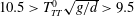 $10.5>T_{TT}^{0}\sqrt{g/d}>9.5$
), the results from H&G are close to the irregular wave results, tending towards the same level, which is
$10.5>T_{TT}^{0}\sqrt{g/d}>9.5$
), the results from H&G are close to the irregular wave results, tending towards the same level, which is
 ${\sim}44\,\%$
below the theory (figure 7
c). Compared to the results on finite depth by Paulsen et al. (Reference Paulsen, Bredmose, Bingham and Jacobsen2014b
) for
${\sim}44\,\%$
below the theory (figure 7
c). Compared to the results on finite depth by Paulsen et al. (Reference Paulsen, Bredmose, Bingham and Jacobsen2014b
) for
 $k_{TT}r=0.1$
, a deviation is observed. However, Kristiansen & Faltinsen (Reference Kristiansen and Faltinsen2017) point at a substantial difference between the forces in deep water and finite depth.
$k_{TT}r=0.1$
, a deviation is observed. However, Kristiansen & Faltinsen (Reference Kristiansen and Faltinsen2017) point at a substantial difference between the forces in deep water and finite depth.
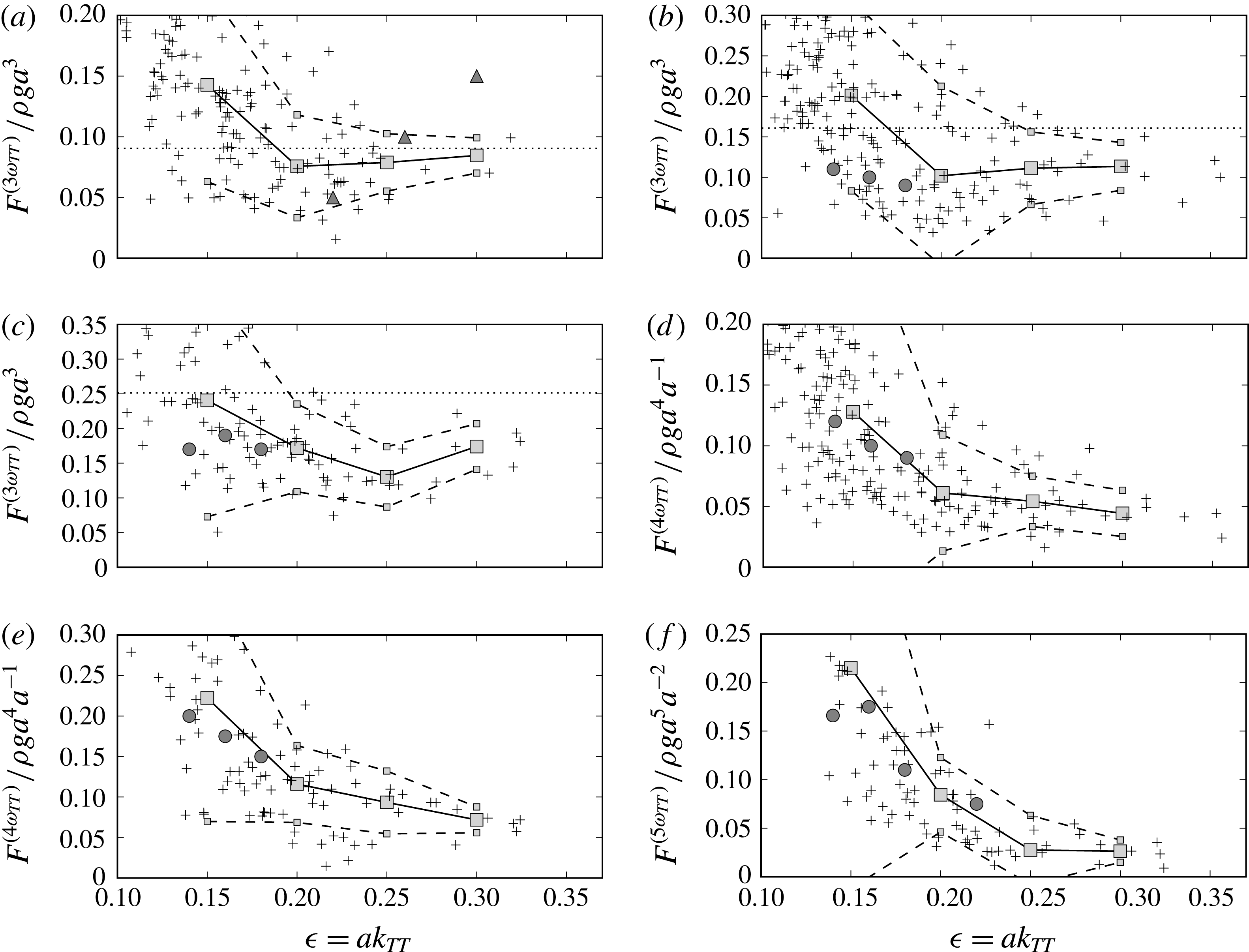
Figure 7. Higher harmonic wave force components. Individual events (
 $+$
), ensemble average (—— ▪) and standard deviation (– – ▪),
$+$
), ensemble average (—— ▪) and standard deviation (– – ▪),
 $F_{FNV}^{(3)}$
(- - -), H&G (●) and Paulsen et al. (Reference Paulsen, Bredmose, Bingham and Jacobsen2014b
) for finite water depth (▴). (a)
$F_{FNV}^{(3)}$
(- - -), H&G (●) and Paulsen et al. (Reference Paulsen, Bredmose, Bingham and Jacobsen2014b
) for finite water depth (▴). (a)
 $F^{(3\unicode[STIX]{x1D714}_{TT})}$
for
$F^{(3\unicode[STIX]{x1D714}_{TT})}$
for
 $0.10\leqslant k_{TT}r\leqslant 0.14$
, (b)
$0.10\leqslant k_{TT}r\leqslant 0.14$
, (b)
 $F^{(3\unicode[STIX]{x1D714}_{TT})}$
for
$F^{(3\unicode[STIX]{x1D714}_{TT})}$
for
 $0.14\leqslant k_{TT}r\leqslant 0.18$
, (c)
$0.14\leqslant k_{TT}r\leqslant 0.18$
, (c)
 $F^{(3\unicode[STIX]{x1D714}_{TT})}$
for
$F^{(3\unicode[STIX]{x1D714}_{TT})}$
for
 $0.18\leqslant k_{TT}r\leqslant 0.22$
, (d)
$0.18\leqslant k_{TT}r\leqslant 0.22$
, (d)
 $F^{(4\unicode[STIX]{x1D714}_{TT})}$
for
$F^{(4\unicode[STIX]{x1D714}_{TT})}$
for
 $0.14\leqslant k_{TT}r\leqslant 0.18$
, (e)
$0.14\leqslant k_{TT}r\leqslant 0.18$
, (e)
 $F^{(4\unicode[STIX]{x1D714}_{TT})}$
for
$F^{(4\unicode[STIX]{x1D714}_{TT})}$
for
 $0.18\leqslant k_{TT}r\leqslant 0.22$
and (f)
$0.18\leqslant k_{TT}r\leqslant 0.22$
and (f)
 $F^{(5\unicode[STIX]{x1D714}_{TT})}$
for
$F^{(5\unicode[STIX]{x1D714}_{TT})}$
for
 $0.18\leqslant k_{TT}r\leqslant 0.22$
.
$0.18\leqslant k_{TT}r\leqslant 0.22$
.
For the fourth harmonic force,
 $F^{(4\unicode[STIX]{x1D714}_{TT})}$
, the results show good agreement with H&G (figure 7(d,e). The results for the fifth harmonic force,
$F^{(4\unicode[STIX]{x1D714}_{TT})}$
, the results show good agreement with H&G (figure 7(d,e). The results for the fifth harmonic force,
 $F^{(5\unicode[STIX]{x1D714}_{TT})}$
, are similar to those of H&G for
$F^{(5\unicode[STIX]{x1D714}_{TT})}$
, are similar to those of H&G for
 $k_{TT}r=0.245$
, where the present results are obtained for the wider range of
$k_{TT}r=0.245$
, where the present results are obtained for the wider range of
 $0.18<k_{TT}r<0.22$
(figure 7
f). A comparison between the normalized forces for
$0.18<k_{TT}r<0.22$
(figure 7
f). A comparison between the normalized forces for
 $\unicode[STIX]{x1D716}=0.25$
is provided in table 2.
$\unicode[STIX]{x1D716}=0.25$
is provided in table 2.
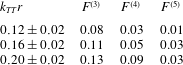
Table 2. The ensemble average of the higher harmonic wave force components
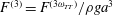 $F^{(3)}=F^{(3\unicode[STIX]{x1D714}_{TT})}/\unicode[STIX]{x1D70C}ga^{3}$
,
$F^{(3)}=F^{(3\unicode[STIX]{x1D714}_{TT})}/\unicode[STIX]{x1D70C}ga^{3}$
,
 $F^{(4)}=F^{(4\unicode[STIX]{x1D714}_{TT})}/\unicode[STIX]{x1D70C}ga^{4}a^{-1}$
and
$F^{(4)}=F^{(4\unicode[STIX]{x1D714}_{TT})}/\unicode[STIX]{x1D70C}ga^{4}a^{-1}$
and
 $F^{(5)}=F^{(5\unicode[STIX]{x1D714}_{TT})}/\unicode[STIX]{x1D70C}ga^{5}a^{-2}$
for local wavenumber
$F^{(5)}=F^{(5\unicode[STIX]{x1D714}_{TT})}/\unicode[STIX]{x1D70C}ga^{5}a^{-2}$
for local wavenumber
 $0.10<k_{TT}r<0.22$
and wave slope
$0.10<k_{TT}r<0.22$
and wave slope
 $\unicode[STIX]{x1D716}=ak_{TT}=0.25$
.
$\unicode[STIX]{x1D716}=ak_{TT}=0.25$
.
The present extracted higher harmonic force components in the irregular waves, for
 $0.1<k_{TT}r<0.22$
and
$0.1<k_{TT}r<0.22$
and
 $0.1<\unicode[STIX]{x1D716}<0.32$
, provide a quite strong generalization of the higher harmonic forces measured by H&G in the regular waves with
$0.1<\unicode[STIX]{x1D716}<0.32$
, provide a quite strong generalization of the higher harmonic forces measured by H&G in the regular waves with
 $0.1<\unicode[STIX]{x1D716}<0.24$
. This in spite of the present results being obtained from the wave-exciting moment, assuming a moment arm equal to the still water level. We note that the present irregular wave results have a significant standard deviation not observed in the regular wave measurements.
$0.1<\unicode[STIX]{x1D716}<0.24$
. This in spite of the present results being obtained from the wave-exciting moment, assuming a moment arm equal to the still water level. We note that the present irregular wave results have a significant standard deviation not observed in the regular wave measurements.
As expected for the third harmonic forces, the FNV approximation is found to best fit the longest waves (
 $0.1<k_{TT}r<0.14$
). In general we observe that the force components are tending towards a constant level for the steep waves. The compliance with the previous results in periodic waves indicates that the high frequency contribution originates from nonlinearities and not from shorter linear free waves, since regular waves do not contain energy from linear free waves. Moreover, it illustrates that the local wave slope and the wavenumber defined in (2.3) are useful proxies of the local wave events.
$0.1<k_{TT}r<0.14$
). In general we observe that the force components are tending towards a constant level for the steep waves. The compliance with the previous results in periodic waves indicates that the high frequency contribution originates from nonlinearities and not from shorter linear free waves, since regular waves do not contain energy from linear free waves. Moreover, it illustrates that the local wave slope and the wavenumber defined in (2.3) are useful proxies of the local wave events.
3.3 Wave load mechanisms
In this section we discuss the following different wave load mechanisms driving the response:
(i) wave-exciting inertia forces, a function of the fluid acceleration;
(ii) wave slamming, due to both non-breaking and breaking wave events;
(iii) the secondary load cycle; and
(iv) possible drag forces as a function of the fluid velocity.
Consider the wave-exciting moment in figure 5(b) where the maximum occurs for
 $t/T_{P}=0$
. This is simultaneous to the maximum wave crest and means that the orbital velocity is approximately horizontal and at maximum. The force at this instant is associated with wave breaking, slamming and possible viscous drag forces (Paulsen et al.
Reference Paulsen, Bredmose, Bingham and Jacobsen2014b
; Kristiansen & Faltinsen Reference Kristiansen and Faltinsen2017) which are included in the categories (ii) and (iv) above.
$t/T_{P}=0$
. This is simultaneous to the maximum wave crest and means that the orbital velocity is approximately horizontal and at maximum. The force at this instant is associated with wave breaking, slamming and possible viscous drag forces (Paulsen et al.
Reference Paulsen, Bredmose, Bingham and Jacobsen2014b
; Kristiansen & Faltinsen Reference Kristiansen and Faltinsen2017) which are included in the categories (ii) and (iv) above.
Consider then the negative response maximum in figure 5(d), of absolute value
 $R^{max}\approx 8\unicode[STIX]{x1D70E}_{M}$
and occurring at
$R^{max}\approx 8\unicode[STIX]{x1D70E}_{M}$
and occurring at
 $t/T_{P}\approx 0.25$
. This is approximately at the same time as the wave elevation has a zero down-crossing, corresponding to a maximum horizontal particle acceleration at the surface. The acceleration is associated with an inertia force and is in accordance with category (i). Returning to the load history in figure 5(b), the secondary load cycle (Grue et al.
Reference Grue, Bjørshol and Strand1993) occurs slightly before the time of the negative response extreme.
$t/T_{P}\approx 0.25$
. This is approximately at the same time as the wave elevation has a zero down-crossing, corresponding to a maximum horizontal particle acceleration at the surface. The acceleration is associated with an inertia force and is in accordance with category (i). Returning to the load history in figure 5(b), the secondary load cycle (Grue et al.
Reference Grue, Bjørshol and Strand1993) occurs slightly before the time of the negative response extreme.
The dynamic part of the response,
 $R(t)-M(t)$
, further highlights the effects of the different load mechanisms (i)–(iv). In figure 5(e) we observe that the large wave crest produces a significant change of the response amplitude and its phase for
$R(t)-M(t)$
, further highlights the effects of the different load mechanisms (i)–(iv). In figure 5(e) we observe that the large wave crest produces a significant change of the response amplitude and its phase for
 $t/T_{P}>0$
. Between the two local response peaks at
$t/T_{P}>0$
. Between the two local response peaks at
 $t/T_{P}\approx -0.1$
and
$t/T_{P}\approx -0.1$
and
 $t/T_{P}\approx 0.1$
the dynamic part experiences a local oscillation of duration equal to half of the resonance period. The modification of the response is due to a strongly nonlinear impulse type of loading, originating from the slamming event. As a result, the dynamic contribution attains a value of
$t/T_{P}\approx 0.1$
the dynamic part experiences a local oscillation of duration equal to half of the resonance period. The modification of the response is due to a strongly nonlinear impulse type of loading, originating from the slamming event. As a result, the dynamic contribution attains a value of
 $R(t)-M(t)\approx 4\unicode[STIX]{x1D70E}_{M}$
at
$R(t)-M(t)\approx 4\unicode[STIX]{x1D70E}_{M}$
at
 $t/T_{P}\approx 0.1$
. The response is further increased to
$t/T_{P}\approx 0.1$
. The response is further increased to
 $R(t)-M(t)\approx 5\unicode[STIX]{x1D70E}_{M}$
around the wave zero down-crossing, at
$R(t)-M(t)\approx 5\unicode[STIX]{x1D70E}_{M}$
around the wave zero down-crossing, at
 $t/T_{P}\approx 0.25$
, with load contributions from the large inertia force and the secondary load cycle. Another effect that adds to the large negative response peak is the restoring force of the cylinder. Even with no wave-exciting forces, this would cause a negative response peak after the positive build-up. The timing of this, relative to the wave forces, is governed by
$t/T_{P}\approx 0.25$
, with load contributions from the large inertia force and the secondary load cycle. Another effect that adds to the large negative response peak is the restoring force of the cylinder. Even with no wave-exciting forces, this would cause a negative response peak after the positive build-up. The timing of this, relative to the wave forces, is governed by
 $\unicode[STIX]{x1D714}_{0}$
, the natural frequency. A result of the different load contributions working together, is that the maximum response occurs after and in the opposite direction of the maximum wave-exciting moment, approximately at the same time as the wave elevation has a zero down-crossing.
$\unicode[STIX]{x1D714}_{0}$
, the natural frequency. A result of the different load contributions working together, is that the maximum response occurs after and in the opposite direction of the maximum wave-exciting moment, approximately at the same time as the wave elevation has a zero down-crossing.
We have now discussed the load event in figure 5. Further, we consider the load histories of the 21 largest response events which are listed in table 3. More specifically, these events are obtained with regards to
 $R^{max}/\unicode[STIX]{x1D70E}_{M}$
for
$R^{max}/\unicode[STIX]{x1D70E}_{M}$
for
 $\unicode[STIX]{x1D714}_{0}/\unicode[STIX]{x1D714}_{P}=3$
. We observe that different wave load and response mechanisms contribute to the response level, including:
$\unicode[STIX]{x1D714}_{0}/\unicode[STIX]{x1D714}_{P}=3$
. We observe that different wave load and response mechanisms contribute to the response level, including:
(i) a large nonlinear inertia force before the wave crest has passed,
 $F_{I,front}$
, which is observed for 15 of the 21 events. The inertia force is characterized by the front of the wave being steep with
$\unicode[STIX]{x0394}\unicode[STIX]{x1D702}/\unicode[STIX]{x0394}t>5H_{S}/T_{P}$
;
$F_{I,front}$
, which is observed for 15 of the 21 events. The inertia force is characterized by the front of the wave being steep with
$\unicode[STIX]{x0394}\unicode[STIX]{x1D702}/\unicode[STIX]{x0394}t>5H_{S}/T_{P}$
;(ii) a large nonlinear inertia force after the wave crest has passed,
$F_{I,back}$
, observed for 16 of 21 events. This is characterized by the back of the wave being steep with
$\unicode[STIX]{x0394}\unicode[STIX]{x1D702}/\unicode[STIX]{x0394}t<-5H_{S}/T_{P}$
;(iii) wave slamming,
$F_{slam}$
, observed for 8 of 21 events, including the 4 largest events. Here slamming is characterized by a coinciding wave crest and a maximum wave-exciting moment; and(iv) the secondary load cycle,
$F_{II}$
, observed for 17 of 21 events. The
$F_{II}$
values are found to coincide with a steep crest back and occur close to the wave zero down-crossing.


Further we note:
(i) an opposite direction of the maximum response,
$R_{opp}$
, characterized by the maximum response occurring after and in the opposite direction to the maximum wave-exciting moment and simultaneous to the wave zero down-crossing. This is observed for 16 out of 21 events;(ii) an effect of a preceding wave,
$\unicode[STIX]{x1D706}_{prec}$
, where the response is affected by the inertia of the moving pile. The oscillations are significant before the wave event appears. This is observed for 7 out of 21 events, where 3 among the 7 events are strongly dominated by the effect.


Table 3. Wave parameters and observed wave load and response characteristics, for the 21 largest response events when
 $\unicode[STIX]{x1D714}_{0}/\unicode[STIX]{x1D714}_{P}=3$
, listed in decreasing order with respect to
$\unicode[STIX]{x1D714}_{0}/\unicode[STIX]{x1D714}_{P}=3$
, listed in decreasing order with respect to
 $R^{max}/\unicode[STIX]{x1D70E}_{M}$
. The characteristics are confirmed with Y
$R^{max}/\unicode[STIX]{x1D70E}_{M}$
. The characteristics are confirmed with Y
 $=$
Yes, N
$=$
Yes, N
 $=$
No or Y(S)
$=$
No or Y(S)
 $=$
Yes, strongly dominated. Parameters in the table: event number, series index, time of occurrence and the rest of the parameters are defined in the text.
$=$
Yes, strongly dominated. Parameters in the table: event number, series index, time of occurrence and the rest of the parameters are defined in the text.
We observe that slamming plays a dominant role for the largest response events. Apart from one of the preceding wave cases, large nonlinear inertia forces are present for all of the events, where either the front or back of the wave, or both, are observed to be steep. However, the large inertia force and the resulting response rather occurs for a large elevation gradient in the back of the wave while what happens in the wave front is less important. Apart from one preceding wave case, the secondary load cycle is found to coincide with the steep wave gradient in the back of the wave.
3.4 Nonlinear versus linear exceedance probability
The empirical exceedance probabilities of the nonlinear wave-exciting moment and motion response are found using (2.2). Each of the series is considered separately, where the frequency ratio is varied with
 $\unicode[STIX]{x1D714}_{0}/\unicode[STIX]{x1D714}_{P}=3,4$
or 5. The load and responses are presented for increasing nonlinearity (
$\unicode[STIX]{x1D714}_{0}/\unicode[STIX]{x1D714}_{P}=3,4$
or 5. The load and responses are presented for increasing nonlinearity (
 $0.10<\unicode[STIX]{x1D716}_{P}<0.14$
) and for long and moderately long waves (
$0.10<\unicode[STIX]{x1D716}_{P}<0.14$
) and for long and moderately long waves (
 $0.09<k_{P}r<0.14$
).
$0.09<k_{P}r<0.14$
).
Estimates for the linear wave-exciting moment and motion response were carried out for reference purposes. In order to estimate the underlying linear wave spectrum, the measured surface elevation was linearized as proposed by Johannessen (Reference Johannessen2010, Reference Johannessen2012). The second-order contribution was calculated from the measured wave time series, using the total surface elevation. Subsequently, the linear surface elevation was found by subtracting the second-order contribution from the measured surface elevation. Further, irregular waves were created from each of the estimated linear wave spectra. The MacCamy & Fuchs solution (Reference MacCamy and Fuchs1954) was used to obtain the wave-exciting moment for a fixed cylinder. More details are found in appendix B.
As expected, the linear and nonlinear analyses agree well for
 $\unicode[STIX]{x1D714}_{0}/\unicode[STIX]{x1D714}_{P}=3$
when the waves are long and have small amplitude (
$\unicode[STIX]{x1D714}_{0}/\unicode[STIX]{x1D714}_{P}=3$
when the waves are long and have small amplitude (
 $\unicode[STIX]{x1D716}_{P}=0.10$
and
$\unicode[STIX]{x1D716}_{P}=0.10$
and
 $k_{P}r=0.09$
, figure 8
a). The same is true when the wave slope is moderate and the waves are long (
$k_{P}r=0.09$
, figure 8
a). The same is true when the wave slope is moderate and the waves are long (
 $\unicode[STIX]{x1D716}_{P}=0.12$
and
$\unicode[STIX]{x1D716}_{P}=0.12$
and
 $k_{P}r=0.09$
, figure 8
b). In these cases the estimated linear response provides a good representation of the nonlinear probability.
$k_{P}r=0.09$
, figure 8
b). In these cases the estimated linear response provides a good representation of the nonlinear probability.
Figure 8. The empirical exceedance probability for the linear wave-exciting moment (– –), nonlinear wave-exciting moment (
 $+$
), linear motion response (——) and nonlinear motion response (○) where
$+$
), linear motion response (——) and nonlinear motion response (○) where
 $\unicode[STIX]{x1D714}_{0}/\unicode[STIX]{x1D714}_{P}=3$
for (a) series a,
$\unicode[STIX]{x1D714}_{0}/\unicode[STIX]{x1D714}_{P}=3$
for (a) series a,
 $(\unicode[STIX]{x1D716}_{P},k_{P}r)=(0.10,0.09)$
,(b) b,
$(\unicode[STIX]{x1D716}_{P},k_{P}r)=(0.10,0.09)$
,(b) b,
 $(0.12,0.09)$
, (c) c,
$(0.12,0.09)$
, (c) c,
 $(0.12,0.11)$
, (d) d,
$(0.12,0.11)$
, (d) d,
 $(0.12,0.14)$
, (e) e,
$(0.12,0.14)$
, (e) e,
 $(0.14,0.09)$
and (f) f,
$(0.14,0.09)$
and (f) f,
 $(0.14,0.14)$
.
$(0.14,0.14)$
.
Figure 9. The empirical exceedance probability for the linear wave-exciting moment (– –), nonlinear wave-exciting moment (
 $+$
), linear motion response (——) and nonlinear motion response (○) where
$+$
), linear motion response (——) and nonlinear motion response (○) where
 $\unicode[STIX]{x1D714}_{0}/\unicode[STIX]{x1D714}_{P}=4$
for (a) series a,
$\unicode[STIX]{x1D714}_{0}/\unicode[STIX]{x1D714}_{P}=4$
for (a) series a,
 $(\unicode[STIX]{x1D716}_{P},k_{P}r)=(0.10,0.09)$
, (b) b,
$(\unicode[STIX]{x1D716}_{P},k_{P}r)=(0.10,0.09)$
, (b) b,
 $(0.12,0.09)$
, (c) c,
$(0.12,0.09)$
, (c) c,
 $(0.12,0.11)$
, (d) d,
$(0.12,0.11)$
, (d) d,
 $(0.12,0.14)$
, (e) e,
$(0.12,0.14)$
, (e) e,
 $(0.14,0.09)$
and (f) f,
$(0.14,0.09)$
and (f) f,
 $(0.14,0.14)$
.
$(0.14,0.14)$
.
For moderate wave slope and moderately long waves (
 $\unicode[STIX]{x1D716}_{P}=0.12$
and
$\unicode[STIX]{x1D716}_{P}=0.12$
and
 $k_{P}r=0.11$
, figure 8
c), the linear estimate gives a good representation of the distribution of the response for
$k_{P}r=0.11$
, figure 8
c), the linear estimate gives a good representation of the distribution of the response for
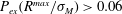 $P_{ex}(R^{max}/\unicode[STIX]{x1D70E}_{M})>0.06$
. However, for
$P_{ex}(R^{max}/\unicode[STIX]{x1D70E}_{M})>0.06$
. However, for
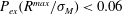 $P_{ex}(R^{max}/\unicode[STIX]{x1D70E}_{M})<0.06$
the nonlinear contribution becomes significant, showing a deviation of
$P_{ex}(R^{max}/\unicode[STIX]{x1D70E}_{M})<0.06$
the nonlinear contribution becomes significant, showing a deviation of
 ${\sim}50\,\%$
for the largest nonlinear response events (marked by circles) when compared to the corresponding linear estimates. For steeper and shorter waves, we observe that the deviation appears at an earlier stage: for
${\sim}50\,\%$
for the largest nonlinear response events (marked by circles) when compared to the corresponding linear estimates. For steeper and shorter waves, we observe that the deviation appears at an earlier stage: for
 $\unicode[STIX]{x1D716}_{P}=0.12$
and
$\unicode[STIX]{x1D716}_{P}=0.12$
and
 $k_{P}r=0.14\,P_{ex}(R^{max}/\unicode[STIX]{x1D70E}_{M})\sim 0.1$
(figure 8
d), for
$k_{P}r=0.14\,P_{ex}(R^{max}/\unicode[STIX]{x1D70E}_{M})\sim 0.1$
(figure 8
d), for
 $\unicode[STIX]{x1D716}_{P}=0.14$
and
$\unicode[STIX]{x1D716}_{P}=0.14$
and
 $k_{P}r=0.09\,P_{ex}(R^{max}/\unicode[STIX]{x1D70E}_{M})\sim 0.2$
(figure 8
e) and for
$k_{P}r=0.09\,P_{ex}(R^{max}/\unicode[STIX]{x1D70E}_{M})\sim 0.2$
(figure 8
e) and for
 $\unicode[STIX]{x1D716}_{P}=0.14$
and
$\unicode[STIX]{x1D716}_{P}=0.14$
and
 $k_{P}r=0.14\,P_{ex}(R^{max}/\unicode[STIX]{x1D70E}_{M})\sim 0.3$
(figure 8
f). For the steepest waves (
$k_{P}r=0.14\,P_{ex}(R^{max}/\unicode[STIX]{x1D70E}_{M})\sim 0.3$
(figure 8
f). For the steepest waves (
 $\unicode[STIX]{x1D716}_{P}=0.14$
) the nonlinear force deviates earlier from the linear force for longer waves (compare figure 8
e,f). We note that while the wave-exciting moment is dominated by the energy around the governing wave frequency, the response is governed by the nonlinear high frequency forces.
$\unicode[STIX]{x1D716}_{P}=0.14$
) the nonlinear force deviates earlier from the linear force for longer waves (compare figure 8
e,f). We note that while the wave-exciting moment is dominated by the energy around the governing wave frequency, the response is governed by the nonlinear high frequency forces.
For
 $\unicode[STIX]{x1D714}_{0}/\unicode[STIX]{x1D714}_{P}=4$
the response for small wave slopes and long waves (
$\unicode[STIX]{x1D714}_{0}/\unicode[STIX]{x1D714}_{P}=4$
the response for small wave slopes and long waves (
 $\unicode[STIX]{x1D716}_{P}=0.10$
and
$\unicode[STIX]{x1D716}_{P}=0.10$
and
 $k_{P}r=0.09$
, figure 9
a) follows the linear results, but shows a deviating trend for small exceedance probability. For moderate wave slope and long waves (
$k_{P}r=0.09$
, figure 9
a) follows the linear results, but shows a deviating trend for small exceedance probability. For moderate wave slope and long waves (
 $\unicode[STIX]{x1D716}_{P}=0.12$
and
$\unicode[STIX]{x1D716}_{P}=0.12$
and
 $k_{P}r=0.09$
, figure 9
b) the deviation between the nonlinear and linear results becomes evident for
$k_{P}r=0.09$
, figure 9
b) the deviation between the nonlinear and linear results becomes evident for
 $P_{ex}\approx 0.1$
. In moderate and steep waves (
$P_{ex}\approx 0.1$
. In moderate and steep waves (
 $\unicode[STIX]{x1D716}_{P}>0.12$
, figure 9
b–f) a significant deviation between the nonlinear and linear results is found for
$\unicode[STIX]{x1D716}_{P}>0.12$
, figure 9
b–f) a significant deviation between the nonlinear and linear results is found for
 $P_{ex}<0.2$
. For
$P_{ex}<0.2$
. For
 $\unicode[STIX]{x1D714}_{0}/\unicode[STIX]{x1D714}_{P}=5$
the same tendencies as for
$\unicode[STIX]{x1D714}_{0}/\unicode[STIX]{x1D714}_{P}=5$
the same tendencies as for
 $\unicode[STIX]{x1D714}_{0}/\unicode[STIX]{x1D714}_{P}=4$
are observed. When the frequency is increased, the response tends towards the wave-exciting moment, which is equivalent with the quasi-static level.
$\unicode[STIX]{x1D714}_{0}/\unicode[STIX]{x1D714}_{P}=4$
are observed. When the frequency is increased, the response tends towards the wave-exciting moment, which is equivalent with the quasi-static level.
As expected, the linear and nonlinear analyses agree well when the waves are long and have small amplitude. The nonlinearity of the wave-exciting moment becomes more important in the steeper and shorter waves. The nonlinearity also becomes more prominent when the frequency ratio
 $\unicode[STIX]{x1D714}_{0}/\unicode[STIX]{x1D714}_{P}$
is increased from 3 to 4.
$\unicode[STIX]{x1D714}_{0}/\unicode[STIX]{x1D714}_{P}$
is increased from 3 to 4.
3.5 Extreme response events
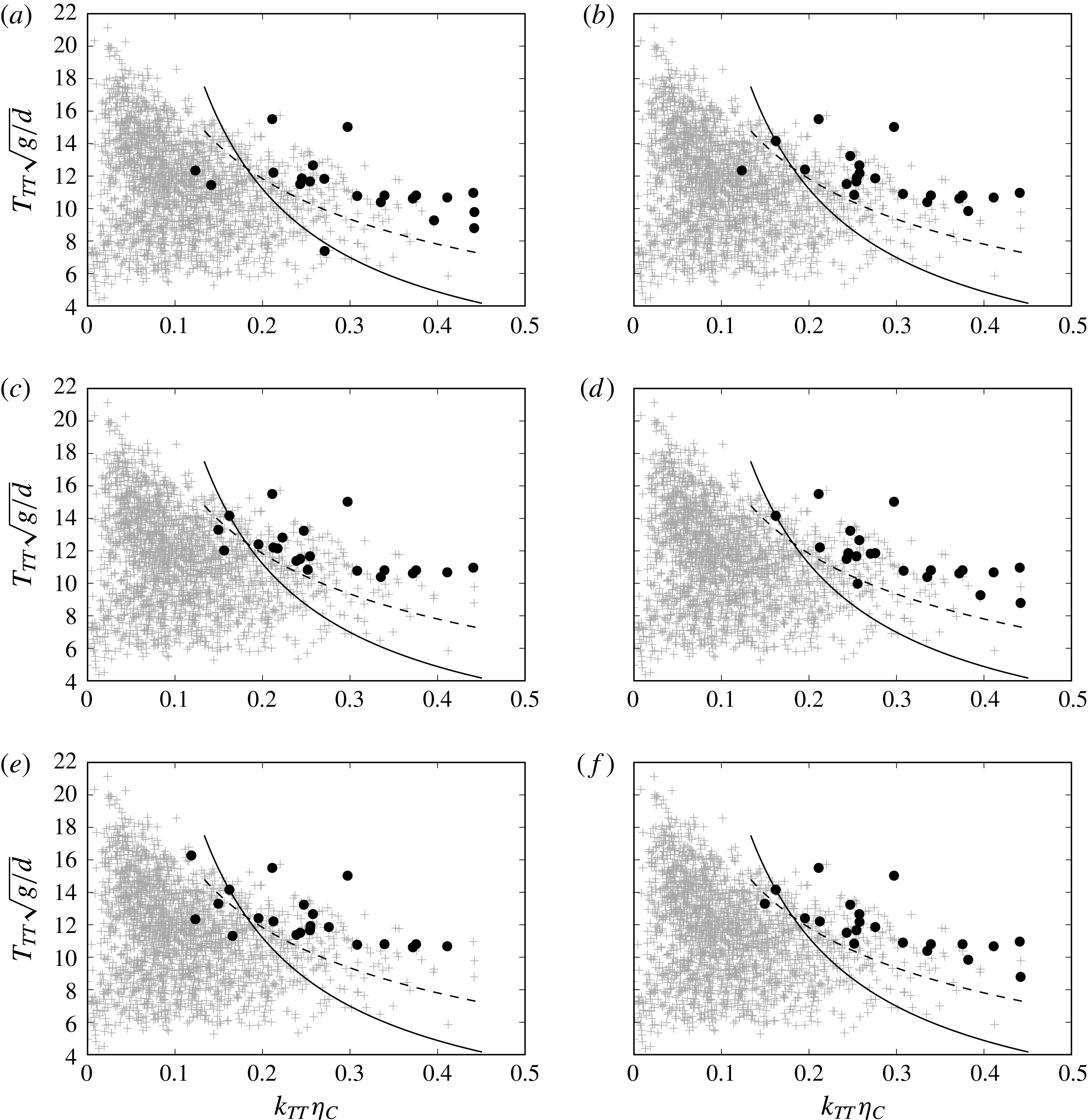
Figure 10. Wave scatter plot including all the 2166 events (
 $+$
), events with
$+$
), events with
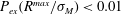 $P_{ex}(R^{max}/\unicode[STIX]{x1D70E}_{M})<0.01$
(●),
$P_{ex}(R^{max}/\unicode[STIX]{x1D70E}_{M})<0.01$
(●),
 $Fr=0.4$
(——) and
$Fr=0.4$
(——) and
 $KC=5$
(– –) for (a)
$KC=5$
(– –) for (a)
 $(\unicode[STIX]{x1D714}_{0}/\unicode[STIX]{x1D714}_{P},\unicode[STIX]{x1D701})=(3,0.02)$
, (b)
$(\unicode[STIX]{x1D714}_{0}/\unicode[STIX]{x1D714}_{P},\unicode[STIX]{x1D701})=(3,0.02)$
, (b)
 $(3,0.06)$
, (c)
$(3,0.06)$
, (c)
 $(4,0.02)$
, (d)
$(4,0.02)$
, (d)
 $(4,0.06)$
, (e)
$(4,0.06)$
, (e)
 $(5,0.02)$
and (f)
$(5,0.02)$
and (f)
 $(5,0.06)$
.
$(5,0.06)$
.
The most extreme responses are critical for design. It is of interest to further investigate the wave effects driving these responses. The 1 % largest events (satisfying
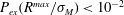 $P_{ex}(R^{max}/\unicode[STIX]{x1D70E}_{M})<10^{-2}$
) are presented in scatter diagrams according to the wave proxies
$P_{ex}(R^{max}/\unicode[STIX]{x1D70E}_{M})<10^{-2}$
) are presented in scatter diagrams according to the wave proxies
 $T_{TT}\sqrt{g/d}$
and
$T_{TT}\sqrt{g/d}$
and
 $k_{TT}\unicode[STIX]{x1D702}_{C}$
. The resonance frequencies are
$k_{TT}\unicode[STIX]{x1D702}_{C}$
. The resonance frequencies are
 $\unicode[STIX]{x1D714}_{0}/\unicode[STIX]{x1D714}_{P}=3,4$
and 5. The majority of these events occur for waves with period
$\unicode[STIX]{x1D714}_{0}/\unicode[STIX]{x1D714}_{P}=3,4$
and 5. The majority of these events occur for waves with period
 $T_{TT}\sqrt{g/d}$
between 9 and 16 and wave slope
$T_{TT}\sqrt{g/d}$
between 9 and 16 and wave slope
 $k_{TT}\unicode[STIX]{x1D702}_{C}$
larger than 0.2 (figure 10
a,c,e).
$k_{TT}\unicode[STIX]{x1D702}_{C}$
larger than 0.2 (figure 10
a,c,e).
In order to discuss the history effect in the response, i.e. the contribution from the inertia of the moving pile due to successive large wave events, we present calculations with a damping of both
 $\unicode[STIX]{x1D701}=0.02$
and
$\unicode[STIX]{x1D701}=0.02$
and
 $\unicode[STIX]{x1D701}=0.06$
, where in the latter the effect of preceding waves, for the local response, is smaller compared to the former. The extreme response events obtained with
$\unicode[STIX]{x1D701}=0.06$
, where in the latter the effect of preceding waves, for the local response, is smaller compared to the former. The extreme response events obtained with
 $\unicode[STIX]{x1D701}=0.06$
all gather in a common region (figure 10
b,d,f).
$\unicode[STIX]{x1D701}=0.06$
all gather in a common region (figure 10
b,d,f).
The nonlinear high frequency forces driving the response originates either from flow separation, free surface gravity waves or a combination. Flow separation is governed by the Keulegan–Carpenter number
 $KC=u_{C}T_{TT}/d$
, while gravity wave effects are governed by the Froude number
$KC=u_{C}T_{TT}/d$
, while gravity wave effects are governed by the Froude number
 $Fr=u_{C}/\sqrt{gd}$
. We have in figure 10 indicated the line corresponding to
$Fr=u_{C}/\sqrt{gd}$
. We have in figure 10 indicated the line corresponding to
 $KC=5$
. Almost all of the extreme events are found for
$KC=5$
. Almost all of the extreme events are found for
 $KC>5$
and
$KC>5$
and
 $k_{TT}\unicode[STIX]{x1D702}_{C}>0.15$
. Note that a
$k_{TT}\unicode[STIX]{x1D702}_{C}>0.15$
. Note that a
 $KC$
-number larger than 2 is commonly associated with flow separation (Sarpkaya Reference Sarpkaya1986).
$KC$
-number larger than 2 is commonly associated with flow separation (Sarpkaya Reference Sarpkaya1986).
A contribution of flow separation to the higher harmonic wave forces has recently been suggested by Paulsen et al. (Reference Paulsen, Bredmose, Bingham and Jacobsen2014b
), Kristiansen & Faltinsen (Reference Kristiansen and Faltinsen2017). We remark that the details of the flow separation depend on the Reynolds number (
 $Re$
) and are different in the model scale compared to the large scale, where
$Re$
) and are different in the model scale compared to the large scale, where
 $Re$
is approximately 1000 times larger. The possible flow separation may contain more three-dimensional effects in the large scale compared to the model scale.
$Re$
is approximately 1000 times larger. The possible flow separation may contain more three-dimensional effects in the large scale compared to the model scale.
We have also indicated the line
 $Fr=0.4$
, where
$Fr=0.4$
, where
 $Fr=u_{C}/\sqrt{gd}$
. The extreme response events found for waves with
$Fr=u_{C}/\sqrt{gd}$
. The extreme response events found for waves with
 $Fr<0.4$
are all affected by preceding waves. The Froude number indicates a gravity wave effect at the scale of the cylinder diameter, where
$Fr<0.4$
are all affected by preceding waves. The Froude number indicates a gravity wave effect at the scale of the cylinder diameter, where
 $Fr=0.4$
corresponds to a local wavelength
$Fr=0.4$
corresponds to a local wavelength
 $\unicode[STIX]{x1D706}_{C}=2\unicode[STIX]{x03C0}u_{C}^{2}/g$
of the local crest velocity
$\unicode[STIX]{x1D706}_{C}=2\unicode[STIX]{x03C0}u_{C}^{2}/g$
of the local crest velocity
 $u_{C}$
with
$u_{C}$
with
 $\unicode[STIX]{x1D706}_{C}\approx d$
contributing to a particular wave–body interaction, as proposed by Grue et al. (Reference Grue, Bjørshol and Strand1993, Reference Grue, Bjørshol, Strand and Ohkusu1994).
$\unicode[STIX]{x1D706}_{C}\approx d$
contributing to a particular wave–body interaction, as proposed by Grue et al. (Reference Grue, Bjørshol and Strand1993, Reference Grue, Bjørshol, Strand and Ohkusu1994).
The present data of the obtained responses show that the extreme events occur for
 $KC>5$
. The regime
$KC>5$
. The regime
 $KC>5$
, is significantly above the separation limit (
$KC>5$
, is significantly above the separation limit (
 $KC>2$
, Sarpkaya Reference Sarpkaya1986), indicating a flow separation effect and contribution from possible drag forces, even though the flow separation itself has not been measured. The findings supports
$KC>2$
, Sarpkaya Reference Sarpkaya1986), indicating a flow separation effect and contribution from possible drag forces, even though the flow separation itself has not been measured. The findings supports
 $KC$
and flow separation as a more relevant criterion for the extreme response events. However, we choose to include the Froude criterion, as the results are not considered sufficient in order to exclude the surface gravity wave effects. The more visible local free surface wave, suggested at the cylinder diameter scale, is for comparison governed by
$KC$
and flow separation as a more relevant criterion for the extreme response events. However, we choose to include the Froude criterion, as the results are not considered sufficient in order to exclude the surface gravity wave effects. The more visible local free surface wave, suggested at the cylinder diameter scale, is for comparison governed by
 $Fr>0.4$
. The free surface effect is very clear in the experiments. The wave may co-interact with the flow separation effects, suggesting that both effects and criteria are relevant.
$Fr>0.4$
. The free surface effect is very clear in the experiments. The wave may co-interact with the flow separation effects, suggesting that both effects and criteria are relevant.
4 Conclusions
The high frequency resonant responses of a weakly damped monopile exposed to irregular deep water waves have been investigated. The response events were obtained accounting for the short-term wave statistics. Experiments were carried out with a single bottom hinged cylinder in two different set-ups. In the first set-up the cylinder was fixed, while in the other it was free to oscillate, yielding both the wave-exciting moment and the motion response. The nonlinearity, peak wavenumber and peak period of the six different wave series were in the ranges:
 $\unicode[STIX]{x1D716}_{p}\sim 0.10{-}0.14$
,
$\unicode[STIX]{x1D716}_{p}\sim 0.10{-}0.14$
,
 $k_{P}r\sim 0.09{-}0.14$
and
$k_{P}r\sim 0.09{-}0.14$
and
 $T_{P}\sqrt{g/d}\sim 12.0{-}14.8$
, respectively, where all quantities are defined in § 2.2.
$T_{P}\sqrt{g/d}\sim 12.0{-}14.8$
, respectively, where all quantities are defined in § 2.2.
By use of a transfer function, the response was calculated from the measured wave-exciting moment of the fixed cylinder. The calculations of the extreme response maxima compare very well with the measured ones. The accuracy is approximately 5 %. The overall agreement is even better when comparing the sorted maxima (the so-called quantiles). This justifies the use of the measured wave-exciting moment in combination with the transfer function, both for estimating the probability distributions and for calculating the response level of the extreme events. The response is then discussed as a function of the resonance frequency
 $\unicode[STIX]{x1D714}_{0}$
, which is varied in the range where
$\unicode[STIX]{x1D714}_{0}$
, which is varied in the range where
 $\unicode[STIX]{x1D714}_{0}/\unicode[STIX]{x1D714}_{P}\sim 3{-}5$
.
$\unicode[STIX]{x1D714}_{0}/\unicode[STIX]{x1D714}_{P}\sim 3{-}5$
.
The empirical short-term exceedance probability distributions of the nonlinear wave-exciting moment and motion response, obtained for each of the six series, show: for small wave slope (
 $\unicode[STIX]{x1D716}_{P}=0.10$
), long waves (
$\unicode[STIX]{x1D716}_{P}=0.10$
), long waves (
 $k_{P}r=0.09$
) and a resonance frequency of
$k_{P}r=0.09$
) and a resonance frequency of
 $\unicode[STIX]{x1D714}_{0}/\unicode[STIX]{x1D714}_{P}=3$
, the nonlinear response analyses agree, and the results in fact are very well represented by their linear counterparts. The same is true for a moderate wave slope (
$\unicode[STIX]{x1D714}_{0}/\unicode[STIX]{x1D714}_{P}=3$
, the nonlinear response analyses agree, and the results in fact are very well represented by their linear counterparts. The same is true for a moderate wave slope (
 $\unicode[STIX]{x1D716}_{P}=0.12$
) and long waves (
$\unicode[STIX]{x1D716}_{P}=0.12$
) and long waves (
 $k_{P}r=0.09$
). By increasing the ratio
$k_{P}r=0.09$
). By increasing the ratio
 $\unicode[STIX]{x1D714}_{0}/\unicode[STIX]{x1D714}_{P}$
to 4 or 5, the importance of the nonlinearities becomes apparent, where the deviation between the nonlinear and linear calculations occurs for an exceedance probability of
$\unicode[STIX]{x1D714}_{0}/\unicode[STIX]{x1D714}_{P}$
to 4 or 5, the importance of the nonlinearities becomes apparent, where the deviation between the nonlinear and linear calculations occurs for an exceedance probability of
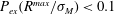 $P_{ex}(R^{max}/\unicode[STIX]{x1D70E}_{M})<0.1$
. For moderate to strong waves (
$P_{ex}(R^{max}/\unicode[STIX]{x1D70E}_{M})<0.1$
. For moderate to strong waves (
 $\unicode[STIX]{x1D716}_{P}\sim 0.12{-}0.14$
) and long to moderately long waves (
$\unicode[STIX]{x1D716}_{P}\sim 0.12{-}0.14$
) and long to moderately long waves (
 $k_{P}r\sim 0.09{-}0.14$
), the deviation between the nonlinear and linear results are clear in all cases. The deviation starts earlier for
$k_{P}r\sim 0.09{-}0.14$
), the deviation between the nonlinear and linear results are clear in all cases. The deviation starts earlier for
 $\unicode[STIX]{x1D714}_{0}/\unicode[STIX]{x1D714}_{P}=4,5$
compared to
$\unicode[STIX]{x1D714}_{0}/\unicode[STIX]{x1D714}_{P}=4,5$
compared to
 $\unicode[STIX]{x1D714}_{0}/\unicode[STIX]{x1D714}_{P}=3$
, as well as for an increasing wave slope, and for a decreasing wavelength.
$\unicode[STIX]{x1D714}_{0}/\unicode[STIX]{x1D714}_{P}=3$
, as well as for an increasing wave slope, and for a decreasing wavelength.
The most extreme response events, moreover, are obtained according to the local wave proxies: the local trough-to-trough period
 $T_{TT}\sqrt{g/d}$
and the local wave slope estimate
$T_{TT}\sqrt{g/d}$
and the local wave slope estimate
 $k_{TT}\unicode[STIX]{x1D702}_{C}$
. The events are found in a region where the Keulegan–Carpenter number exceeds
$k_{TT}\unicode[STIX]{x1D702}_{C}$
. The events are found in a region where the Keulegan–Carpenter number exceeds
 $KC>5$
, indicating that possible flow separation effects contribute to the extreme responses. The contribution of flow separation to the higher harmonic wave forces has been recently suggested by Paulsen et al. (Reference Paulsen, Bredmose, Bingham and Jacobsen2014b
), Kristiansen & Faltinsen (Reference Kristiansen and Faltinsen2017). A similar region is also covered by a Froude number exceeding
$KC>5$
, indicating that possible flow separation effects contribute to the extreme responses. The contribution of flow separation to the higher harmonic wave forces has been recently suggested by Paulsen et al. (Reference Paulsen, Bredmose, Bingham and Jacobsen2014b
), Kristiansen & Faltinsen (Reference Kristiansen and Faltinsen2017). A similar region is also covered by a Froude number exceeding
 $Fr>0.4$
pointing to surface gravity wave effects at the scale of the cylinder diameter, as suggested by Grue et al. (Reference Grue, Bjørshol and Strand1993, Reference Grue, Bjørshol, Strand and Ohkusu1994). It is still an open research question whether either of the effects are dominant or if they are of equal importance.
$Fr>0.4$
pointing to surface gravity wave effects at the scale of the cylinder diameter, as suggested by Grue et al. (Reference Grue, Bjørshol and Strand1993, Reference Grue, Bjørshol, Strand and Ohkusu1994). It is still an open research question whether either of the effects are dominant or if they are of equal importance.
From a number of large response events, different wave load mechanisms are discussed: (i) wave-exciting inertia forces, a function of the fluid acceleration; (ii) wave slamming due to both non-breaking and breaking wave events; (iii) the secondary load cycle; and (iv) possible drag forces as a function of the fluid velocity.
The third, fourth and fifth harmonic wave-exciting force components are extracted by their ensemble average and standard deviation in the irregular waves. They are expressed by the local wave proxies. The present results, for a wave slope up to 0.3, fit well to, and generalize, the results in regular waves for a wave slope up to 0.24 of Huseby & Grue (Reference Huseby and Grue2000). The third harmonic force in the longer waves shows good agreement with the FNV method.
The JONSWAP spectrum was chosen to approximate a real ocean environment. In general, the findings are expected to apply for a broader range of storm conditions, i.e. other spectral shapes. However, one should be careful when there is the possibility of a linearly induced high frequency response, such as in combined wind and swell sea, i.e. two peak spectra.
Acknowledgements
This study was carried out with financial support from Stiftelsen Det Norske Veritas, DNV GL and The Research Council of Norway. The technical assistance during the experimental work by Head Engineer Olav Gundersen is gratefully acknowledged.
Appendix A
The vertical cylinder may rotate with an angle
 $\unicode[STIX]{x1D703}(t)$
in the pitch mode of motion about a hinge at the bottom, located at
$\unicode[STIX]{x1D703}(t)$
in the pitch mode of motion about a hinge at the bottom, located at
 $z=z_{0}=2~\text{cm}$
above the tank floor. Assuming linear motion, the moment due to the pressure forces with respect to
$z=z_{0}=2~\text{cm}$
above the tank floor. Assuming linear motion, the moment due to the pressure forces with respect to
 $z_{0}$
reads:
$z_{0}$
reads:
 $M_{wave}(t)-a_{55}\ddot{\unicode[STIX]{x1D703}}-b_{55}\dot{\unicode[STIX]{x1D703}}-c_{55}\unicode[STIX]{x1D703}$
, where
$M_{wave}(t)-a_{55}\ddot{\unicode[STIX]{x1D703}}-b_{55}\dot{\unicode[STIX]{x1D703}}-c_{55}\unicode[STIX]{x1D703}$
, where
 $M_{wave}(t)$
,
$M_{wave}(t)$
,
 $a_{55}$
,
$a_{55}$
,
 $b_{55}$
and
$b_{55}$
and
 $c_{55}$
denote the wave exciting moment, added mass, damping and restoring coefficients in the pitch mode of motion, respectively. The moment due to the spring forces reads:
$c_{55}$
denote the wave exciting moment, added mass, damping and restoring coefficients in the pitch mode of motion, respectively. The moment due to the spring forces reads:
 $-(z_{a}-z_{0})(F_{2}(t)-F_{1}(t))=-\unicode[STIX]{x1D705}_{0}(z_{a}-z_{0})^{2}\unicode[STIX]{x1D703}$
where
$-(z_{a}-z_{0})(F_{2}(t)-F_{1}(t))=-\unicode[STIX]{x1D705}_{0}(z_{a}-z_{0})^{2}\unicode[STIX]{x1D703}$
where
 $z_{a}$
denotes the height of the force transducers,
$z_{a}$
denotes the height of the force transducers,
 $F_{1}(t)$
and
$F_{1}(t)$
and
 $F_{2}(t)$
denote the force recorded on the left and right transducer, respectively, see figure 4, and
$F_{2}(t)$
denote the force recorded on the left and right transducer, respectively, see figure 4, and
 $\unicode[STIX]{x1D705}_{0}$
the spring constant. Balance of angular momentum gives
$\unicode[STIX]{x1D705}_{0}$
the spring constant. Balance of angular momentum gives
 $$\begin{eqnarray}m_{55}\ddot{\unicode[STIX]{x1D703}}=-a_{55}\ddot{\unicode[STIX]{x1D703}}-b_{55}\dot{\unicode[STIX]{x1D703}}-(\unicode[STIX]{x1D705}_{0}(z_{a}-z_{0})^{2}+c_{55})\unicode[STIX]{x1D703}+M_{wave}(t),\end{eqnarray}$$
where
 $m_{55}$
denotes the moment of inertia of the water filled cylinder. This yields
$m_{55}$
denotes the moment of inertia of the water filled cylinder. This yields
 $$\begin{eqnarray}\ddot{\unicode[STIX]{x1D703}}+2\unicode[STIX]{x1D701}\unicode[STIX]{x1D714}_{0}\dot{\unicode[STIX]{x1D703}}+\unicode[STIX]{x1D714}_{0}^{2}\unicode[STIX]{x1D703}=M_{wave}(t)/(m_{55}+a_{55}),\end{eqnarray}$$
where the resonance frequency is given by
 $\unicode[STIX]{x1D714}_{0}^{2}=(c_{55}+\unicode[STIX]{x1D705}_{0}(z_{a}-z_{0})^{2})/(m_{55}+a_{55})$
. Note that the spring force provides the dominant contribution to the restoring force where
$\unicode[STIX]{x1D714}_{0}^{2}=(c_{55}+\unicode[STIX]{x1D705}_{0}(z_{a}-z_{0})^{2})/(m_{55}+a_{55})$
. Note that the spring force provides the dominant contribution to the restoring force where
 $c_{55}$
is 0.005 times
$c_{55}$
is 0.005 times
 $\unicode[STIX]{x1D705}_{0}(z_{a}-z_{0})^{2}$
for the actual cylinder. The still water decay tests as well as the irregular wave experiments determine
$\unicode[STIX]{x1D705}_{0}(z_{a}-z_{0})^{2}$
for the actual cylinder. The still water decay tests as well as the irregular wave experiments determine
 $\unicode[STIX]{x1D714}_{0}=17.7~\text{rad}~\text{s}^{-1}$
of the oscillating cylinder. The damping ratio
$\unicode[STIX]{x1D714}_{0}=17.7~\text{rad}~\text{s}^{-1}$
of the oscillating cylinder. The damping ratio
 $\unicode[STIX]{x1D701}$
, determined as the fraction of the critical damping, is 0.02 for the cylinder. In the experiments with the fixed cylinder set-up, small vibrations are measured at frequencies
$\unicode[STIX]{x1D701}$
, determined as the fraction of the critical damping, is 0.02 for the cylinder. In the experiments with the fixed cylinder set-up, small vibrations are measured at frequencies
 $\unicode[STIX]{x1D714}>88~\text{rad}~\text{s}^{-1}$
. These are driven by the wavemaker and transferred through the tank frame to the cylinder set-up.
$\unicode[STIX]{x1D714}>88~\text{rad}~\text{s}^{-1}$
. These are driven by the wavemaker and transferred through the tank frame to the cylinder set-up.
Equation (A 2) may be expressed in matrix form:
 $(\text{d}/\text{d}t)(\text{e}^{\boldsymbol{A}t}Y)=\text{e}^{\boldsymbol{A}t}[0,M_{wave}(t)/(m_{55}+a_{55})\unicode[STIX]{x1D714}_{\unicode[STIX]{x1D701}}]^{\text{T}}$
where
$(\text{d}/\text{d}t)(\text{e}^{\boldsymbol{A}t}Y)=\text{e}^{\boldsymbol{A}t}[0,M_{wave}(t)/(m_{55}+a_{55})\unicode[STIX]{x1D714}_{\unicode[STIX]{x1D701}}]^{\text{T}}$
where
 $Y=[\unicode[STIX]{x1D703},y]^{\text{T}}$
,
$Y=[\unicode[STIX]{x1D703},y]^{\text{T}}$
,
 $[\,]^{\text{T}}$
denotes the transpose,
$[\,]^{\text{T}}$
denotes the transpose,
 $\dot{\unicode[STIX]{x1D703}}+\unicode[STIX]{x1D701}\unicode[STIX]{x1D714}_{0}\unicode[STIX]{x1D703}=\unicode[STIX]{x1D714}_{\unicode[STIX]{x1D701}}y$
, and
$\dot{\unicode[STIX]{x1D703}}+\unicode[STIX]{x1D701}\unicode[STIX]{x1D714}_{0}\unicode[STIX]{x1D703}=\unicode[STIX]{x1D714}_{\unicode[STIX]{x1D701}}y$
, and
 $\unicode[STIX]{x1D714}_{\unicode[STIX]{x1D701}}=\unicode[STIX]{x1D714}_{0}\sqrt{1-\unicode[STIX]{x1D701}^{2}}$
. The matrix
$\unicode[STIX]{x1D714}_{\unicode[STIX]{x1D701}}=\unicode[STIX]{x1D714}_{0}\sqrt{1-\unicode[STIX]{x1D701}^{2}}$
. The matrix
 $\unicode[STIX]{x1D63C}$
and its variant
$\unicode[STIX]{x1D63C}$
and its variant
 $\text{e}^{\boldsymbol{A}t}$
are expressed by
$\text{e}^{\boldsymbol{A}t}$
are expressed by
 $$\begin{eqnarray}\unicode[STIX]{x1D63C}=\left(\begin{array}{@{}cc@{}}\unicode[STIX]{x1D701}\unicode[STIX]{x1D714}_{0} & -\unicode[STIX]{x1D714}_{\unicode[STIX]{x1D701}}\\ \unicode[STIX]{x1D714}_{\unicode[STIX]{x1D701}} & \unicode[STIX]{x1D701}\unicode[STIX]{x1D714}_{0}\end{array}\right),\quad \text{e}^{\boldsymbol{A}t}=\text{e}^{\unicode[STIX]{x1D701}\unicode[STIX]{x1D714}_{0}t}\left(\begin{array}{@{}cc@{}}\cos \unicode[STIX]{x1D714}_{\unicode[STIX]{x1D701}}t & -\sin \unicode[STIX]{x1D714}_{\unicode[STIX]{x1D701}}t\\ \sin \unicode[STIX]{x1D714}_{\unicode[STIX]{x1D701}}t & \cos \unicode[STIX]{x1D714}_{\unicode[STIX]{x1D701}}t\end{array}\right).\end{eqnarray}$$
By integration, the pitch angle
 $\unicode[STIX]{x1D703}(t)$
is obtained as a function of time. For convenience this is multiplied by
$\unicode[STIX]{x1D703}(t)$
is obtained as a function of time. For convenience this is multiplied by
 $\unicode[STIX]{x1D705}_{0}(z_{a}-z_{0})^{2}$
giving the moment of the sum spring force with respect to
$\unicode[STIX]{x1D705}_{0}(z_{a}-z_{0})^{2}$
giving the moment of the sum spring force with respect to
 $z_{0}$
. We denote this quantity by
$z_{0}$
. We denote this quantity by
 $R(\unicode[STIX]{x1D714}_{0},t)$
where
$R(\unicode[STIX]{x1D714}_{0},t)$
where
 $$\begin{eqnarray}R(\unicode[STIX]{x1D714}_{0},t)=\unicode[STIX]{x1D705}_{0}(z_{a}-z_{0})^{2}\unicode[STIX]{x1D703}(t)=\frac{\unicode[STIX]{x1D714}_{0}^{2}}{\unicode[STIX]{x1D714}_{\unicode[STIX]{x1D701}}}\int _{0}^{t}M_{wave}(\unicode[STIX]{x1D70F})\text{e}^{-\unicode[STIX]{x1D701}\unicode[STIX]{x1D714}_{0}(t-\unicode[STIX]{x1D70F})}\sin (\unicode[STIX]{x1D714}_{\unicode[STIX]{x1D701}}(t-\unicode[STIX]{x1D70F}))\,\text{d}\unicode[STIX]{x1D70F}.\end{eqnarray}$$
Appendix B
In order to estimate the underlying linear wave spectrum the measured surface elevation,
 $\unicode[STIX]{x1D702}$
, is linearized as proposed by Johannessen (Reference Johannessen2010, Reference Johannessen2012). The second-order contribution,
$\unicode[STIX]{x1D702}$
, is linearized as proposed by Johannessen (Reference Johannessen2010, Reference Johannessen2012). The second-order contribution,
 $\unicode[STIX]{x1D702}^{\prime (2)}$
, is calculated using finite depth theory (Sharma & Dean Reference Sharma and Dean1981), where only nearby wave components are allowed to interact. This is implemented by a maximum bandwidth between the interacting wave components
$\unicode[STIX]{x1D702}^{\prime (2)}$
, is calculated using finite depth theory (Sharma & Dean Reference Sharma and Dean1981), where only nearby wave components are allowed to interact. This is implemented by a maximum bandwidth between the interacting wave components
 $\unicode[STIX]{x1D6FF}\unicode[STIX]{x1D714}=0.8\unicode[STIX]{x1D714}_{P}$
. The prime denotes the use of the total surface elevation for the calculations of the second-order contribution. Then the resulting linear surface elevation,
$\unicode[STIX]{x1D6FF}\unicode[STIX]{x1D714}=0.8\unicode[STIX]{x1D714}_{P}$
. The prime denotes the use of the total surface elevation for the calculations of the second-order contribution. Then the resulting linear surface elevation,
 $\unicode[STIX]{x1D702}^{(1)}$
, is found by
$\unicode[STIX]{x1D702}^{(1)}$
, is found by
 $$\begin{eqnarray}\unicode[STIX]{x1D702}-\unicode[STIX]{x1D702}^{\prime (2)}=(\unicode[STIX]{x1D702}^{(1)}+\unicode[STIX]{x1D702}^{(2)}+\cdots \,)-(\unicode[STIX]{x1D702}^{\prime (2)}+O^{(3)})=\unicode[STIX]{x1D702}^{(1)}+O^{(3)}\end{eqnarray}$$
being accurate to and including second-order effects. Subsequently, theoretical realizations of irregular waves were created from each of the linear wave spectra, with random phase. The MacCamy & Fuchs solution (Reference MacCamy and Fuchs1954) was used to obtain the linear wave-exciting moment for a fixed cylinder. The standard deviation of the linear part is, on average for the six series, 1 % smaller than the measured and fully nonlinear wave-exciting moment. Finally, the response transfer function (A 4) was used to calculate the linear motion response.


