2. Direct numerical simulation

With the Oberbeck–Boussinesq approximation, the dimensionless governing equations for incompressible turbulent RBC flow are

(2.1)\begin{gather} \hat{\boldsymbol{\nabla}}\boldsymbol{\cdot}\hat{\boldsymbol{u}}=0, \end{gather}

(2.2)\begin{gather}\partial_{\hat{t}}\hat{\boldsymbol{u}}+(\hat{\boldsymbol{u}}\boldsymbol{\cdot} \hat{\boldsymbol{\nabla}})\hat{\boldsymbol{u}} ={-}\hat{\boldsymbol{\nabla}}\hat{p}+\frac{1}{\sqrt{Ra/Pr}} \hat{\nabla}^{2}\hat{\boldsymbol{u}}+\hat{\theta}\boldsymbol{e}_{\hat{z}}, \end{gather}

(2.3)\begin{gather}\partial_{\hat{t}}\hat{\theta}+(\hat{\boldsymbol{u}} \boldsymbol{\cdot}\hat{\boldsymbol{\nabla}})\hat{\theta} =\frac{1}{\sqrt{Ra\,Pr}}\hat{\nabla}^{2}\hat{\theta}. \end{gather}

The dimensionless fields of velocity $\hat {\boldsymbol {u}}$, temperature $\hat {\theta }$ and pressure $\hat {p}$, as well as length and time, are in the units of the free-fall velocity $U_{f}=\sqrt {\alpha g H \varDelta }$, the applied temperature difference $\varDelta$, the free-fall pressure $p_{f}=\rho \alpha g H \varDelta$, the sample height $H$ and the free-fall time $T_{f}=\sqrt {H/(\alpha g \varDelta )}$, respectively.

We used a finite-difference code to solve the above governing equations. The DNS code has been used and described in detail in previous studies (Bao et al. Reference Bao, Chen, Liu, She, Zhang and Zhou2015; Chen et al. Reference Chen, Bao, Yin and She2017; Zhang et al. Reference Zhang, Sun, Bao and Zhou2018). Here we only mention some of the key information. The Rayleigh numbers were in the range $10^{6} \leqslant Ra \leqslant 10^{10}$ and the Prandtl number $Pr = 4.3$. The DNS were performed in three RBC samples of different geometries. One of them was a 3-D cuboid, as shown in figure 1(a), with length $L = H$, width $W = H/4$ and resulting aspect ratios $\varGamma _x \equiv L/H=1$ and $\varGamma _y \equiv W/H = 1/4$. The other two were 2-D rectangles with aspect ratios $\varGamma = L/H = 1$ and $10$, respectively. Figure 1(b) shows the schematic diagram of the slip length $b$ for the horizontal conducting plate. In all simulations, the horizontal plates were set to be slippery with $b \geqslant 0$, and the sidewalls were no-slip and adiabatic. All boundaries are rigid and impermeable. Thus, the dimensionless boundary conditions are given by

(2.4)\begin{gather} \hat{\boldsymbol{u}}\big|_{{sidewalls}}=0 , \end{gather}

(2.5)\begin{gather}\boldsymbol{n}\boldsymbol{\cdot}\hat{\boldsymbol{\nabla}} \hat{\theta}\big|_{{sidewalls}}=0, \end{gather}

(2.6)\begin{gather}\hat{u}\big|_{horizontal\, plates}=\hat{b}\partial_{\hat{z}}\hat{u} , \end{gather}

(2.7)\begin{gather}\hat{v}\big|_{horizontal\, plates}=\hat{b}\partial_{\hat{z}}\hat{v}, \end{gather}

(2.8)\begin{gather}\hat{w}\big|_{horizontal\, plates}= 0, \end{gather}

(2.9a,b)\begin{gather}\hat{\theta}\big|_{{bottom}}=0.5 , \quad \hat{\theta}\big|_{top}={-}0.5 , \end{gather}

where $\hat {b} = b/H$ is the dimensionless slip length, and $\hat {u}$, $\hat {v}$ and $\hat {w}$ are, respectively, the velocity components along the $x$, $y$ and $z$ directions.

Figure 1. (a) Schematic diagram of the 3-D turbulent RBC sample used for numerical simulation. The dimensions of the sample are $L:H:W = 4:4:1$. (b) Schematic diagram of the slip length $b$ and the velocity $u_s =b(\partial u/\partial n)_s$ on the surface.

In the simulation, the governing equations were discretised by employing a conservative second-order central difference on a staggered grid in space. The time-derivative terms were discretised by the (implicit) backward Euler method. The diffusive terms were solved by an implicit scheme and the convective terms were solved by an explicit scheme. Inside the thermal BL, we used a small mesh size of $4\times 10^{-4}\,H$ to ensure that there are at least 20 grid points to resolve the thermal BL. Outside the BL, we used a larger mesh size of $2\times 10^{-3}\,H$ uniformly distributed along both the $x$ and $z$ directions. In all simulations, the initial conditions ($t = 0$) were set to ${\hat {\boldsymbol {u}}} = 0$ and $\hat {\theta } = 0$.

We calculated the dimensionless heat transport, the Nusselt number $Nu$, using $Nu \equiv \sqrt {Ra\,Pr}\,\langle \hat {w} \hat {\theta } \rangle _{V,t} +1$. Here $\langle \cdot \rangle _{V,t}$ denotes volume and time averaging. In each simulation, we waited for a long enough time in the unit of $T_f$ (${\gtrsim }100 T_f$) so that the system reached a statistically steady state, and conducted time averaging after that (see table 2 in the Appendix). The overall running time ensured that all the averages are convergent. The minimum grid spacing was smaller than the dimensionless Kolmogorov length scale $\eta _K=\sqrt {Pr}/[Ra(Nu-1)]^{1/4}$ and the Batchelor length scale $\eta _B=1/[Ra(Nu-1)]^{1/4}$ (Shishkina et al. Reference Shishkina, Stevens, Grossmann and Lohse2010), which ensured adequate spatial resolution. Details of the DNS parameters can be found in table 2.

3. Global heat transport $Nu$ for varying slip length $b$

Figure 2 shows typical snapshots of temperature fields (a,c,e) and velocity fields (b,d,f) for different values of $b$. The results are obtained from the 2-D sample with $\varGamma = 1$ and $Ra = 10^{9}$. For a plate of finite $b$, as shown in panels (a–d), the LSC of the fluid has a tilted single-roll mode with its axis along the sample diagonal. For free-slip plates, however, one can find a stable double-roll mode of the LSC – one roll on top of the other – in panels (e) and (f).

Figure 2. Snapshots of instantaneous (a,c,e) temperature and (b,d,f) velocity fields for no-slip plates (a,b), slippery plates with $b/\lambda _0 = 1.02$ (c,d) and free-slip plates (e,f). The DNS data are obtained for the 2-D RBC sample with $\varGamma = 1$ at $Ra=10^{9}$.

For comparison, as shown in figure 3, the LSC state for the 3-D sample remains the single-roll mode for both the no-slip and free-slip plates. Recent investigations for no-slip RBC revealed that the single-roll mode for water ($Pr \simeq 5$) can slightly enhance the heat transport compared to the double-roll mode (Xi & Xia Reference Xi and Xia2008; Weiss & Ahlers Reference Weiss and Ahlers2011, Reference Weiss and Ahlers2013), and the enhancement becomes more prominent in low-$Pr$ fluids and for multiple-roll LSC due to elliptical instability (Zwirner & Shishkina Reference Zwirner and Shishkina2018; Zwirner, Tilgner & Shishkina Reference Zwirner, Tilgner and Shishkina2020). With a similar mechanism, one would expect in free-slip RBC that the double-roll mode also transports less heat than the single-roll mode.

Figure 3. Snapshots of temperature and velocity fields in the 3-D sample with $\varGamma _y = 1/4$ and $Ra=10^{9}$ for (a) no-slip plates, (b) slippery plates with $b/\lambda _0 = 1.02$ and (c) free-slip plates. The obtained fields are in the vertical plane of $y/W = 0.6$.

Figures 4(a) and 4(b) show, respectively, typical snapshots of the temperature and velocity fields from the 2-D sample with $\varGamma = 10$ and $Ra = 10^{9}$ for different $b$. For no-slip cases, as shown in figures 4(a1) and 4(b1), the number of LSC rolls $R_n$ increases when $\varGamma$ is stretched, and they form a stable multiple-roll mode – one roll next to the other – that filled up the closed sample. When $R_n$ increases by 1, van der Poel et al. (Reference van der Poel, Stevens, Sugiyama and Lohse2012) revealed that $Nu$ increases by the amount of $\Delta Nu^{R_n+1}_{R_n}$, the value of which decreases as $\varGamma$ increases until it saturates at a large $\varGamma$. For $Ra = 10^{8}$ and $\varGamma = 10$, our data show that $\Delta Nu^{R_n+1}_{R_n}$ is $2.5\,\%$ of $Nu$, which agrees well with the previous results by van der Poel et al. (Reference van der Poel, Stevens, Sugiyama and Lohse2012). For $Ra = 10^{9}$, we find that $\Delta Nu^{R_n+1}_{R_n}$ is $1.4\,\%$ of $Nu$. Thus, the influence of the LSC roll number, if any, accounts for only a few per cent of $Nu$ and decreases as $Ra$ increases. With the fixed initial conditions of ${\hat {\boldsymbol {u}}} = 0$ and $\hat {\theta } = 0$, we found that the LSC roll number is rather stable and it rarely changes over the whole averaging time (see table 2).

Figure 4. Snapshots of (a1–a3) temperature and (b1–b3) velocity fields obtained from the 2-D sample with $\varGamma = 10$ and $Ra=10^{9}$. Results are for (a1,b1) no-slip plates, (a2,b2) slippery plates with $b/\lambda _0=1.02$ and (a3,b3) free-slip plates.

Figure 4(a2) and 4(b2) are the results for slippery plates with $b/\lambda _0=1.02$. It is found that $R_n$ decrease as $b$ increases. When the plates are free-slip, figures 4(a3) and 4(b3) show that the multiple-roll mode vanishes and the convection flow forms a single-roll circulation that spans the whole interior bulk region. Compared to the zonal flow that was observed in the DNS of free-slip RBC using a horizontally periodic boundary condition (Goluskin et al. Reference Goluskin, Johnston, Flierl and Spiegel2014; Wang et al. Reference Wang, Chong, Stevens, Verzicco and Lohse2020a), the single-roll LSC can move up and down along the vertical sidewalls. This flow motion helps enhance the vertical heat transport compared to the zonal flow, and thus yields higher efficiency of heat transport.

Now, we discuss the dependence of heat transport $Nu$ on the slip length $b$. Figure 5(a) shows the reduced $Nu/Ra^{0.312}$ as a function of $Ra$ obtained from the three closed samples for different values of the normalised $b/H$. We chose the scaling $Ra^{0.312}$ since it was well established in the classical RBC regime for $10^{9} \lesssim Ra \lesssim 10^{12}$ (Ahlers et al. Reference Ahlers, He, Funfschilling and Bodenschatz2012b; He et al. Reference He, Funfschilling, Nobach, Bodenschatz and Ahlers2012b). One can see in figure 5(a) that the classical scaling also roughly holds for different aspect ratios and for different values of $b/H$: only the prefactor increases as $b/H$ increases, and reaches the maximal value when the plates are free-slip. The data (see table 2) show that the scalings of $Nu_F(Ra)$ for free-slip RBC in 2-D and 3-D are nearly the same, differing only by a constant factor. This is a consistent extension of previous results for no-slip RBC (van der Poel, Stevens & Lohse Reference van der Poel, Stevens and Lohse2013).

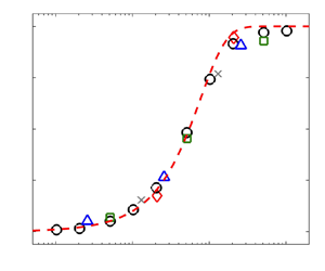
Figure 5. (a) Plot of $Nu/Ra^{0.312}$ as a function of $Ra$ from 2-D and 3-D DNS for different $\varGamma$ and $b/H$. Symbols correspond to $\varGamma = 1$ with no-slip plates (red open circles), $b/H=10^{-3}$ (grey crosses), $b/H = 10^{-2}$ (black open diamonds), $b/H = 10^{-1}$ (green stars) and free-slip plates (red solid circles). Blue open (solid) triangles are for $\varGamma = 10$ with no-slip (free-slip) plates. Red open (solid) squares are for $\varGamma _y = 1/4$ with no-slip (free-slip) plates. (b) Plot of $Nu_F/Nu_0$ as a function of $Ra$ in 2-D and 3-Dsamples for $\varGamma = 1$ (black circles), $\varGamma = 10$ (blue triangles) and $\varGamma _y = 1/4$ (red squares). (c) Plot of $Nu/Nu_0$ as a function of $b/\lambda _0$ on a logarithmic scale. The DNS data are obtained in the 2-D sample with $\varGamma = 1$ for varying $Ra=10^{6}$ (grey crosses), $10^{7}$ (blue triangles), $10^{8}$ (green squares), $10^{9}$ (black circles) and $10^{10}$ (red diamonds). The red dashed line represents the function $Nu/Nu_0=N_{0} \tanh (b/\lambda _0)+1$, with $N_{0}=0.8$. Here $Nu_0$ and $Nu_F$ represent the normalised heat flux for no-slip and free-slip plates, respectively; and $\lambda _0 \equiv H/(2Nu_0)$ is the thermal BL thickness accordingly.

We plot in figure 5(b) the ratio $Nu_F/Nu_0$ as a function of $Ra$ for different $\varGamma$. Here $Nu_0$ and $\mbox { {Nu}}_F$ represent the normalised heat flux for no-slip and free-slip plates, respectively. In the 2-D sample with $\varGamma = 1$, we find $Nu_F/Nu_0 \simeq 1.8$ nearly independent of $Ra$, and the ratio is ${\sim }6\,\%$ lower than those in the other two samples, where the LSC for free-slip plates remains the single-roll mode. As discussed above, such small deviations are largely attributed to different roll modes of the LSC, while the effects of the slippery plates on $Nu$ are essentially the same in both 2-D and 3-D closed RBC.

Figure 5(c) shows the results for $Nu/Nu_0$ with $\varGamma = 1$. It is found that the $Nu$ data for different $Ra$ and $b$ collapse onto a single master curve once $b$ is rescaled by $\lambda _0$. Here $\lambda _0 \equiv H/(2Nu_0)$ is the thermal BL thickness for no-slip plates. Over the studied parameter range, all the $Nu/Nu_0$ data closely follow the function $Nu/Nu_0=N_{0} \tanh (b/\lambda _0)+1$, with $N_{0} = 0.8 \pm 0.03$.

4. Temperature boundary-layer profiles in slippery RBC

4.1. Equations of the mean temperature and temperature variance profiles

In this section, we derive equations for the dimensionless profiles of the mean temperature $\varTheta$ and temperature variance $\varOmega$ near the BL in slippery RBC. The method is based on the ideas in previous studies for no-slip RBC (Shishkina et al. Reference Shishkina, Horn, Wagner and Ching2015; Wang et al. Reference Wang, Xu, He, Yik, Wang, Schumacher and Tong2018).

We consider a quasi-2-D convective flow over an infinite horizontal plate. With the Reynolds decomposition and the BL approximation, one obtains the mean temperature BL equation,

(4.1)\begin{equation} \langle u\rangle\partial_x \langle \theta\rangle+ (\langle w\rangle-\partial_z\kappa_t)\partial_z \langle \theta\rangle = (\kappa+\kappa_t)\partial^{2}_z \langle \theta \rangle , \end{equation}

with the eddy thermal diffusivity

(4.2)\begin{equation} \kappa_t ={-}\langle w^{\prime}\theta^{\prime}\rangle/\partial_z \langle\theta\rangle. \end{equation}

Here and below, $\langle \cdot \rangle$ denotes average over time; $\langle \theta \rangle$, $\langle u\rangle$ and $\langle w\rangle$ are long-time averages of temperature, horizontal velocity and vertical velocity, respectively; and $\theta ^{\prime }(x,z,t)$, $u^{\prime }(x,z,t)$ and $w^{\prime }(x,z,t)$ are their fluctuations. For an incompressible fluid, the continuity equation is

(4.3)\begin{equation} \partial_x u^{\prime}+\partial_z w^{\prime} = 0 . \end{equation}

On the slippery plate with $z=0$ and $b>0$, both $\theta ^{\prime }$ and $v^{\prime }$ vanish, while $u^{\prime }$ and $\partial _x u^{\prime }$ exist, leading to $\partial _z w^{\prime } \neq 0$. Thus, one has

(4.4)\begin{equation} \langle w^{\prime}\theta^{\prime}\rangle = \partial_z\langle w^{\prime}\theta^{\prime}\rangle = 0 \end{equation}

and

(4.5)\begin{equation} \partial^{2}_z\langle w^{\prime}\theta^{\prime}\rangle \neq 0 . \end{equation}

Using the dimensionless length $\xi =z/\lambda$, with $\lambda \equiv H/(2Nu)$ being the thermal BL thickness near the slippery plate, one finds that $\kappa _t$ and its derivatives with respect to $\xi$ vanish at the plate, i.e.

(4.6a,b)\begin{equation} \kappa_t\big|_{\xi=0}=(\kappa_t)_{\xi}\big|_{\xi=0}=0 , \quad (\kappa_t)_{\xi\xi}\big|_{\xi=0} \neq 0 . \end{equation}

For small $\xi$, $\kappa _t$ can be approximated by

(4.7)\begin{equation} \kappa_t/\kappa \approx m\xi^{p}, \end{equation}

with a dimensionless constant $m > 0$ and an effective exponent $p \geqslant 2$ varying with the degree of slippage. For $Pr > 1$, the solution of (4.1) is given by (Shishkina et al. Reference Shishkina, Horn, Wagner and Ching2015)

(4.8)\begin{equation} \varTheta(\xi) \equiv \frac{\theta_{bottom} - \langle\theta(\xi)\rangle}{\varDelta/2} = \int_0^{\xi}(1+m\eta^{p})^{{-}c}\,{\rm d}\eta , \end{equation}

where $c \geqslant 1$ is a parameter satisfying $\varTheta (\infty ) = 1$, and thus

(4.9)\begin{equation} m = [\varGamma(1/p)\varGamma(c-1/p)/(p\varGamma(c))]^{p} , \end{equation}

where $\varGamma (\cdot )$ denotes the gamma function. It is noteworthy that (4.7) to (4.9) determine a general form of the mean temperature profiles $\varTheta (\xi )$ in slippery RBC with different $b$. When $b \rightarrow \infty$ for free-slip plates, the leading term in (4.7) yields $p = 2$. When $b = 0$, all terms in (4.6a,b) vanish on the no-slip plates at $\xi = 0$. It leads to $p = 3$ and the corresponding $\varTheta (\xi )$ profiles that are the same as the previous results found by Shishkina et al. (Reference Shishkina, Horn, Wagner and Ching2015). In a more general case, the value of $p$ is expected to be between $2$ and $3$.

The dimensionless form of temperature variance $\eta = \langle \theta '^{2} \rangle$ is defined by

(4.10)\begin{equation} \varOmega \equiv \eta /\eta_0 . \end{equation}

Here $\eta _0$ is the maximal value of $\eta$. In the BL, the equation of $\varOmega$ is given by (Wang et al. Reference Wang, He and Tong2016)

(4.11)\begin{equation} \eta_0(\langle u \rangle\partial_x\varOmega + \langle w \rangle \partial_z\varOmega) - 2\kappa_t(\partial_z \langle \theta \rangle)^{2} - \partial_z(\kappa_f\partial_z\eta) = \kappa\eta_0\partial_z^{2}\varOmega - 2\epsilon _\theta , \end{equation}

with the thermal dissipation rate

(4.12)\begin{equation} \epsilon_\theta=\kappa[\langle (\partial_x\theta')^{2}\rangle + \langle (\partial_z\theta')^{2}\rangle] \end{equation}

and the turbulent diffusivity for temperature variance,

(4.13)\begin{equation} \kappa_f ={-}\langle w^{\prime}\theta'^{2}\rangle / \partial_z\eta. \end{equation}

Since both $\theta ^{\prime }$ and ${\theta ^{\prime 2}}$ are advected by the same local velocity $u^{\prime }$, one would expect that the effects of the BL fluctuations on them are similar. Thus on the slippery plates at $\xi = 0$, $\kappa _f$ can be approximated by

(4.14)\begin{equation} \kappa_f/\kappa \approx n\xi^{p}, \end{equation}

with the prefactor $n > 0$.

Using (4.14) and the mean temperature equation (4.8) above, one can write the three terms on the left-hand side of (4.11) as follows:

(4.15)\begin{gather} \eta_0(\langle u\rangle\partial_x \varOmega+\langle w \rangle\partial_z\varOmega) ={-}\dfrac{\eta_0\kappa}{\lambda^{2}}\beta\xi^{p-1}\dfrac{{\rm d}\varOmega(\xi)} {{\rm d}\xi}, \end{gather}

(4.16)\begin{gather}-2\kappa_t (\partial_z \langle\theta\rangle)^{2} ={-}\kappa\dfrac{\varDelta^{2}}{2\lambda^{2}} \dfrac{m\xi^{p}}{(1+m\xi^{p})^{2c}} \end{gather}

and

(4.17)\begin{equation} -\partial_z(\kappa_f\partial_z\eta) ={-}np\xi^{p-1}\kappa\eta_0\dfrac{\partial\varOmega(\xi)}{\partial\xi}\, \dfrac{1}{\lambda^{2}} -n\xi^{p}\kappa\eta_0\dfrac{\partial^{2}\varOmega(\xi)}{\partial\xi^{2}}\, \dfrac{1}{\lambda^{2}}, \end{equation}

where $\beta = pm(c-1)$.

The right-hand side of (4.11) can be written as

(4.18)\begin{equation} \kappa\eta_0\partial_z^{2}\varOmega =\kappa\eta_0\dfrac{\partial^{2}\varOmega(\xi)}{\partial\xi^{2}}\,\dfrac{1}{\lambda^{2}} \end{equation}

and

(4.19)\begin{equation} -2\epsilon_\theta ={-}2\kappa\dfrac{\eta_0}{\lambda^{2}} \left[\dfrac{1}{4}\dfrac{[{\rm d}\varOmega(\xi)/{\rm d}\xi]^{2}} {\varOmega(\xi)}+\gamma\varOmega(\xi)\right] . \end{equation}

Here $\gamma =2\lambda ^{2}({1}/{l_x^{2}}+{1}/{l_z^{2}})$, with $l_x$ and $l_z$ being the Taylor microscales of temperature fluctuations in the $x$ and $z$ directions, respectively.

Taking (4.15) to (4.19) into (4.11), one obtains a general ordinary differential equation of $\varOmega$ for slippery RBC:

(4.20)\begin{align} &(1+n\xi^{p})\frac{{\rm d}^{2}\varOmega(\xi)}{{\rm d}\xi^{2}} +(\beta+np)\xi^{p-1}\frac{{\rm d}\varOmega(\xi)}{{\rm d}\xi} -\frac{[{\rm d}\varOmega(\xi)/{\rm d}\xi]^{2}}{2\varOmega(\xi)} \nonumber\\ &\quad +\frac{\varDelta^{2}}{2\eta_0}\,\frac{m\xi^{p}}{(1+m\xi^{p})^{2c}} -2\gamma\varOmega(\xi)=0. \end{align}

Note that for $p = 3$, (4.20) is equivalent to equation (20) in Wang et al. (Reference Wang, He and Tong2016) for no-slip plates.

With the initial conditions $\varOmega (\xi _0)=1$ and ${\rm d} \varOmega (\xi _0)/{\rm d}\xi =0$ at the peak position $\xi _0$ of $\varOmega (\xi )$, (4.20) yields the solution $\varOmega (\xi; p, c,\varDelta ^{2}/\eta _0,n,\gamma )$ for the general form of temperature variance profiles $\varOmega (\xi )$ near the plate. The values of the maximal normalised temperature variance $\varDelta ^{2}/\eta _0$ and the peak position $\xi _0$ can be obtained directly from the temperature data. The values of $\gamma \simeq 1$ and $\xi _0 \simeq 0.85$ were found for $Pr = 4.4$ and $7.6$ in 3-D experiments and DNS (Wang et al. Reference Wang, He and Tong2016, Reference Wang, Xu, He, Yik, Wang, Schumacher and Tong2018), and they depend weakly on $Pr$ and the sample geometry. The parameters $p$, $c$ and $n$ are determined by the fits of (4.7), (4.8) and (4.14) to the temperature data.

4.2. DNS data for the mean temperature and temperature variance

Figure 6(a) shows the normalised turbulent diffusivities $\kappa _t/\kappa$ for the temperature fluctuation $\theta ^{\prime }$ as a function of $\xi$. The DNS data were obtained from the 2-D sample with $\varGamma = 1$ and the 3-D sample with $\varGamma _y = 1/4$. Over the studied $Ra$ range $10^{6} \leqslant Ra \leqslant 10^{10}$, the $\kappa _t/\kappa$ data from different samples fall into two distinct groups: one for no-slip plates and the other for free-slip plates. For $\xi \lesssim 1$, we find the two groups of data closely follow the power function $\kappa _t/\kappa = m \xi ^{p}$ from (4.7) with different values of $m$ and $p$. For no-slip plates, the value $p = 3$ is consistent with previous DNS results obtained in a 3-D cylindrical sample (Shishkina et al. Reference Shishkina, Horn, Wagner and Ching2015) and a thin disk (Wang et al. Reference Wang, Xu, He, Yik, Wang, Schumacher and Tong2018). The value $m = 0.85$ is close to the thin disk ($m = 0.8$), but about 1.5 times lower than the cylindrical sample, indicating relatively less BL fluctuations in the 2-D or quasi-2-D convection flows. For free-slip plate, our result shows $p = 2$, which agrees with the predicted value in § 4.1.

Figure 6. Normalised turbulent diffusivities (a) $\kappa _t/\kappa$ and (b) $\kappa _f/\kappa$ as a function of $\xi$ in logarithmic scales for no-slip (NS) and free-slip (FS) horizontal plates. The DNS data are obtained from the 2-D sample with $\varGamma = 1$ and the 3-D sample with $\varGamma _y = 1/4$ for different $Ra$. The two lines in panel (a) represent the power function $\kappa _t/\kappa = m\xi ^{p}$ with the parameters $m = 0.73$, $p=2$ (red solid line) and $m = 0.85$, $p=3$ (blue dashed line). In panel (b) they represent the power function $\kappa _f/\kappa = n\xi ^{p}$ with $n = 0.85$, $p=2$ (red solid line) and $n = 1.13$, $p=3$ (blue dashed line).

Figure 6(b) shows the results of normalised turbulent diffusivity $\kappa _f/\kappa$ for the temperature variance ${\theta ^{\prime 2}}$ obtained from the same simulations as those for $\kappa _t/\kappa$. It is found that the $\kappa _f/\kappa$ data in the two RBC samples for different $Ra$ also fall into two groups. Over the range $\xi \lesssim 1$, the no-slip data closely follow the power function $\kappa _f/\kappa = 1.13 \xi ^{3}$, which is consistent with the previous results in the thin disk (Wang et al. Reference Wang, Xu, He, Yik, Wang, Schumacher and Tong2018). For free-slip plates, the $\kappa _f/\kappa$ data are found to be well described by the power function $\kappa _f/\kappa = 0.85 \xi ^{2}$.

Figures 7(a) and (b) show similar results of $\kappa _t/\kappa$ and $\kappa _f/\kappa$, respectively, for different values of $b$. All the data were obtained from the 2-D sample with $\varGamma = 1$ and $Ra = 10^{9}$. In both panels, the diffusivities are compensated by $\xi ^{2}$ in order to present an enlarged view of their evolution as the dimensionless slip length $b/H$. In the BL for $\xi \lesssim 0.6$, both $\kappa _t/\kappa$ and $\kappa _f/\kappa$ follow a power-law scaling of $\xi ^{p}$, with the exponent $p$ varying monotonically from $3$ to $2$ as $b/H$ increases from $0$ to $\infty$. For a given $b$, one sees that the scaling exponents for both diffusivities are the same. This is consistent with the assumption made above, in which the BL fluctuations have similar effects on both $\theta ^{\prime }$ and ${\theta ^{\prime 2}}$.

Figure 7. Normalised turbulent diffusivities (a) $\kappa _t/\kappa$ and (b) $\kappa _f/\kappa$ as a function of $\xi$ for slippery horizontal plates with varying $b/H$. The DNS data are obtained from the 2-D sample with $\varGamma = 1$ and $Ra = 10^{9}$. The symbols in the two panels indicate data for different values of $b/H = 0$ (red circles), $5\times 10^{4}$ (blue squares), $10^{-3}$ (grey triangles), $10^{-2}$ (green pluses) and for free-slip plates (black diamonds). The lines in the two panels represent the power functions $\kappa _t/\kappa = m\xi ^{p}$ and $\kappa _f/\kappa = n\xi ^{p}$, respectively, with the effective exponent (from top to bottom near the left edge) $p = 2.0$, $2.3$, $2.5$, $2.7$ and $3.0$.

Thus, both figures 6 and 7 show that the turbulent diffusivities $\kappa _t/\kappa$ and $\kappa _f/\kappa$ in the BL can be approximated by the power-law scaling in (4.7) and (4.14), respectively. For different values of $b$, we obtain the exponent $p$ from the fits of (4.7) and (4.14) to the $\varGamma = 1$ data in the range $10^{7} \leqslant Ra \leqslant 10^{10}$, and show $p$ as a function of $b/\lambda _0$ in figure 8. The result shows that for $b/\lambda _0 \lesssim 0.03$ the obtained exponent $p = 3$, which indicates that the temperature BL profiles remain roughly the same as those for no-slip plates. In the range $0.03 \lesssim b/\lambda _0 \lesssim 10$, the exponent decreases monotonically from $p = 3$ to $p = 2$ as $b/\lambda _0$ increases. This demonstrates a gradual change of the BL fluctuation intensity from no-slip to free-slip boundaries. The accompanying $Nu$ increment, as shown in figure 5(c), accounts for ${\sim }97\,\%$ of the total heat flux increment due to the boundary condition change. When $b/\lambda _0$ is beyond $10$, we have $p = 2$, and in this case the temperature BL profiles, as well as the heat flux, are nearly the same as those for free-slip plates.

Figure 8. Dependence of the exponent $p$ on the normalised slip length $b/\lambda _0$ in semi-log scales. The DNS data are obtained in the $\varGamma = 1$ sample with different $Ra=10^{7}$ (blue triangles), $10^{8}$ (green squares), $10^{9}$ (black circles) and $10^{10}$ (red diamonds).

Table 1 lists the exponent $p$ and other equation parameters for different $b/\lambda _0$. With these values, one can calculate the general equations for the mean temperature profiles $\varTheta (\xi )$ and the temperature variance profiles $\varOmega (\xi )$ using (4.8) and (4.20), respectively.

Table 1. Values of the parameters used to calculate $\varTheta (\xi )$ and $\varOmega (\xi )$ that are shown in figures 9 and 10.

Figure 9. Plots of (a) $\varTheta$ and (b) $\varOmega$ as functions of $\xi$ obtained in the DNS for different $Ra$ from the 2-D sample with $\varGamma = 1$ and the 3-D sample with $\varGamma _y = 1/4$. The red solid and blue dashed lines in panel (a) represent the calculated $\varTheta (\xi )$ using (4.8). In panel (b), they are the numerical solutions $\varOmega (\xi ; p, c, \varDelta ^{2}/\eta _0, n, \gamma )$ of (4.20) with $\xi _0 = 0.85$. The values of the parameters used to calculate $\varTheta (\xi )$ and $\varOmega (\xi )$ are listed in table 1.

Figure 10. Similar results as in figure 9 for (a) $\varTheta$ and (b) $\varOmega$, obtained from the 2-D samples with $\varGamma = 1$ and $10$. The various symbols in the two panels correspond to different $\varGamma$ and $b/\lambda _0$: red diamonds, $\varGamma =10$, free-slip plates; green squares, $\varGamma = 1$, $b/\lambda _0 =1.02$; black triangles, $\varGamma = 1$, $b/\lambda _0 =0.10$; and blue circles, $\varGamma = 10$, no-slip plates. The lines in panel (a) represent (4.8), and those in panel (b) are the solutions $\varOmega (\xi; p,c,\varDelta ^{2}/\eta _0,n,\gamma )$ of (4.20) with $\xi _0 = 0.85$. The inset in panel (a) shows an enlarged view. The values of the parameters used to calculate $\varTheta (\xi )$ and $\varOmega (\xi )$ are listed in table 1. All the data are obtained at $Ra = 10^{9}$ and $Pr = 4.3$.

Finally, we turn to the DNS results for the mean temperature $\varTheta$ and temperature variance $\varOmega$, and examine the predicted equations for their BL profiles. Figure 9(a) shows $\varTheta (\xi )$ as a function of $\xi$ obtained from the 2-D sample with $\varGamma = 1$ and the 3-D sample with $\varGamma _y = 1/4$ at different $Ra$. It is found that the $\varTheta (\xi )$ data fall into two groups – one for no-slip plates and the other for free-slip plates – both independent of $Ra$ and the sample geometry. With the values of $m$ and $p$ obtained from figure 6(a), we calculated the $\varTheta (\xi )$ curves using the predicted equations (4.8) and (4.9), and plot them in figure 9(a). It is clearly seen that, for either no-slip or free-slip plates, the calculated $\varTheta (\xi )$ curve can well describe the DNS data for $\xi$ up to $3$.

Figure 9(b) shows the corresponding $\varOmega (\xi )$ as a function of $\xi$ from the same DNS as in figure 9(a). Similar to the results of $\varTheta (\xi )$, the $\varOmega (\xi )$ profiles for no-slip and free-slip plates are overlapped respectively onto two separate groups, which are independent of $Ra$ and the sample shape. The two groups of datasets have nearly the same peak position $\xi _0 = 0.85$. In figure 9(b), we also plot the numerical solutions $\varOmega (\xi ; p, c,\varDelta ^{2}/\eta _0,n,\gamma )$ of (4.20) with $\xi _0 = 0.85$ and the other parameters listed in table 1. It is seen that the predicted $\varOmega (\xi )$ curves for no-slip and free-slip plates can well fit the corresponding DNS data for $\xi \lesssim 1.5$. Beyond $\xi \simeq 2$, the predicted curves start to deviate from the data because the power-law scaling of $\kappa _f/\kappa$ no longer holds.

To further examine the predicted general temperature equations (4.8) and (4.20) for slippery plates, we show in figures 10(a) and 10(b), respectively, the $\varTheta (\xi )$ and $\varOmega (\xi )$ BL profiles for varying slip lengths $b/\lambda _0$. All the DNS temperature data were obtained from the 2-D samples with $\varGamma = 1$ and $10$ at $Ra = 10^{9}$. We also calculated the $\varTheta (\xi )$ and $\varOmega (\xi )$ data from (4.8) and (4.20) with the parameters listed in table 1, and plot them in figures 10(a) and 10(b), respectively. Excellent agreements are found between the predicted temperature BL profiles and the temperature data for varying $\varGamma$ and $b/\lambda _0$. It is noted that all the parameters used in the temperature equations depend only on the slip length $b$, and there are no additional adjustable parameters in the calculations of $\varTheta (\xi )$ and $\varOmega (\xi )$. As summarised in table 1, the peak position $\xi _0$ for $\varOmega (\xi )$ remains the same, while all other parameters in the predicted temperature forms change monotonically with $b/\lambda _0$.

In figure 10(a), one sees that the $\varTheta (\xi )$ BL profiles obtained from the $\varGamma = 10$ sample for both no-slip and free-slip plates agree well with the corresponding $\varTheta (\xi )$ curves calculated using (4.8). The calculated $\varTheta (\xi )$ curves are the same as those in figure 9(a) for the other two samples. Similar agreements are also found in figure 10(b) for the $\varOmega (\xi )$ data. The results indicate that the influences of the slippery plates on both mean temperature and temperature variance profiles remain the same in the three samples over the studied $Ra$ range. One would expect that such influences have a weak dependence on the sample geometry and $Ra$, but rather would be dominated by the slip length of the plates. Thus the predicted equations (4.8) and (4.20) for the temperature BL profiles are expected to be valid in a class of thermal convection flows with slippery conducting plates.

5. Summary

We have carried out a systematic DNS study of the Nusselt number and the temperature BL profiles in turbulent Rayleigh–Bénard convection with slippery horizontal conducting plates. The slip length $b$ of the plates varied from $0$ for no-slip to $\infty$ for free-slip plates. The DNS were conducted in the $Ra$ range $10^{6} \leqslant Ra \leqslant 10^{10}$ and for a fixed $Pr = 4.3$. Three closed samples were used in the DNS. One is a 3-D cuboid sample with the dimension of $L:H:W = 4:4:1$ and the other two are 2-D rectangular samples with $\varGamma = 1$ and $10$, respectively.

For a given $b>0$, the obtained $Nu$ data for slippery RBC approximately follow the classical $Nu$ scaling that is observed in no-slip RBC, differing only by an increasing prefactor as $b$ increases. The reduced heat transport $Nu / Nu_0$ from the three samples for different $Ra$ and $b$ can be overlapped onto a single master curve, once the slip length $b$ is normalised by the thermal BL thickness $\lambda _0 \equiv H/(2Nu_0)$. Our DNS results show that the overlapped $Nu/Nu_0$ data follow the scaling $Nu / Nu_0 = N_0 \tanh ( b/\lambda _0) + 1$, with $N_0 = 0.8 \pm 0.03$. This indicates that the slip length can be used as an appropriate characteristic length scale to calculate the heat transport enhancement in slippery RBC.

Near the BL, we calculated the turbulent diffusivities $\kappa _t$ for the temperature fluctuations $\theta ^{\prime }$ and $\kappa _f$ for the temperature variance ${\theta ^{\prime 2}}$. The data were obtained from the three closed samples for different $Ra$ and $b$. It is found that both $\kappa _t$ and $\kappa _f$ can be approximated by a power-law scaling ${\sim }\xi ^{p}$, with an effective scaling exponent $p$ varying from $3$ for no-slip to $2$ for free-slip plates. These results suggest that the influences of BL fluctuations on both $\theta ^{\prime }$ and ${\theta ^{\prime 2}}$ are similar, and show the evolution of such influences as a varying slip length. For $b/\lambda _0 \lesssim 0.03$, we find $p = 3$ and the corresponding temperature profiles $\varTheta (\xi )$ and $\varOmega (\xi )$ remain roughly the same as those for no-slip plates. In the range $0.03 \lesssim b/\lambda _0 \lesssim 10$, our results indicate that the BL fluctuation intensity gradually increases from no-slip to free-slip cases, which accounts for ${\sim }97\,\%$ of the total $Nu$ enhancement as $b/\lambda _0$ increases. When $b/\lambda _0 \gtrsim 10$, the obtained $\varTheta (\xi )$, $\varOmega (\xi )$ and $Nu$ are nearly the same as those for free-slip plates. The analytical relationship between the exponent $p$ and the slip length $b$ is worthy of further investigations in the future.

From these findings, we derived general equations (4.8) and (4.20) for the temperature BL profiles of $\varTheta$ and $\varOmega$, respectively, in slippery RBC with $b \geqslant 0$. When $b = 0$, the predicted temperature BL profiles are consistent with previous results for no-slip RBC (Shishkina et al. Reference Shishkina, Horn, Wagner and Ching2015; Wang et al. Reference Wang, He and Tong2016). When $b>0$, they are in excellent agreement with our DNS data obtained from different samples with varying $Ra$ and $b$. Our work thus provides general functional forms of $Nu/Nu_0$, $\varTheta$ and $\varOmega$ across the BL in slippery RBC. The predicted forms represent the essential effects from the slippery plates on the heat transport and temperature BL profiles, which have weak dependence on the sample geometry and $Ra$ in the studied range. We expect that these scaling forms can be applied to a class of thermal convection flows with slippery conducting plates, ranging from industrial applications to geophysical turbulence.