


1. Introduction
Density differences associated with lateral temperature, salinity or sediment concentration gradients frequently trigger the formation of gravity currents, a class of predominantly horizontal flows that are ubiquitous in the natural environment. Examples concern such phenomena as thunderstorm outflows, haboobs, sea-breeze fronts, flows over sills, turbidity currents and plumes from desalination plants (Simpson Reference Simpson1999; Ungarish Reference Ungarish2009; Meiburg & Kneller Reference Meiburg and Kneller2010).
The central role that gravity currents play in a wide range of environmental settings and technical applications has motivated an extensive body of theoretical, computational and laboratory studies, along with detailed field measurements. A majority of these have focused on flows propagating over smooth, horizontal boundaries, such as the lock-exchange experiments by Huppert & Simpson (Reference Huppert and Simpson1980), Shin, Dalziel & Linden (Reference Shin, Dalziel and Linden2004), Marino, Thomas & Linden (Reference Marino, Thomas and Linden2005) and Adduce, Sciortino & Proietti (Reference Adduce, Sciortino and Proietti2011), as well as corresponding large-scale simulations by Härtel, Meiburg & Necker (Reference Härtel, Meiburg and Necker2000), Cantero, Balachandar & Garcia (Reference Cantero, Balachandar and Garcia2007), Oezgoekmen, Iliescu & Fischer (Reference Oezgoekmen, Iliescu and Fischer2009), Ooi, Constantinescu & Weber (Reference Ooi, Constantinescu and Weber2009) and Rocca et al. (Reference Rocca, Adduce, Lombardi, Sciortino and Hinkelmann2012), among others. These studies demonstrate the existence of different stages in the life of a gravity current. Following the initial collapse, the current undergoes a slumping phase characterized by a constant front velocity. Once there is insufficient fluid left in the lock to maintain this front speed, the current decelerates, until eventually viscous effects become dominant and slow the current down further.
Motivated by applications in which gravity currents propagate over a complex bottom topography, several recent studies have addressed the effects of rough boundaries in such flows. The experiments by Peters & Venart (Reference Peters and Venart2000), in which dense fluid is injected through an inlet entry box, show a slower slumping phase velocity as compared to a smooth bed, along with an earlier onset of the viscous phase. The authors, furthermore, observe enhanced fluid mixing close to the bottom boundary. These findings are consistent with the large-eddy simulations (LES) of Tokyay, Constantinescu & Meiburg (Reference Tokyay, Constantinescu and Meiburg2011), who find that the current speed decays more quickly when the bottom roughness exerts an increased drag force on the current. Nasr-Azadani & Meiburg (Reference Nasr-Azadani and Meiburg2014) employ direct numerical simulations to investigate the three-dimensional vortical flow structures generated when a turbidity current propagates over topographical features such as a Gaussian bump, along with their effects on mixing and entrainment. The recent LES simulations by Bhaganagar & Pillalamarri (Reference Bhaganagar and Pillalamarri2017) address lock-exchange currents over square and triangular roughness elements, with a special emphasis on the role of the friction Reynolds number. Ozan, Constantinescu & Hogg (Reference Ozan, Constantinescu and Hogg2015) highlight the role of dilution in gravity currents propagating over arrays with horizontal axes. Wilson, Friedrich & Stevens (Reference Wilson, Friedrich and Stevens2017) find that a rectangular obstacle initially increases the entrainment of ambient fluid into the current, whereas during the subsequent re-establishment phase this entrainment rate decreases below that of a smooth bed current.
Qualitatively different behaviour is observed for high Reynolds number flows propagating over terrain that is both rough and porous. Several investigations address stratified and homogeneous flows through emergent canopies (Huq et al. Reference Huq, White, Carrillo, Redondo, Dharmavaram and Hanna2007; Belcher, Harman & Finnigan Reference Belcher, Harman and Finnigan2012; Nepf Reference Nepf2012). These exert increased drag on the current and significantly modify its turbulence properties. Cenedese, Nokes & Hyatt (Reference Cenedese, Nokes and Hyatt2018) explore the role of arrays of vertical circular cylinders on gravity currents. For large periodic spacings between the cylinders they find that the currents travel through the cylinder arrays, while for dense arrays they propagate over the top. Ottolenghi, Cenedese & Adduce (Reference Ottolenghi, Cenedese and Adduce2017) find that similar regimes exist when the rough boundary is sloping and with the presence of rotation. They additionally note that both the roughness and the slope of the bed increase entrainment of ambient fluid into the current. Zhou et al. (Reference Zhou, Cenedese, Williams, Ball, Venayagamoorthy and Nokes2017) identify additional flow regimes when the cylinders are non-equidistant. Zhang & Nepf (Reference Zhang and Nepf2011) and Yuksel-Ozan, Constantinescu & Nepf (Reference Yuksel-Ozan, Constantinescu and Nepf2016) find similar behaviour in the context of buoyant gravity currents interacting with floating cylinders.
The present investigation focuses on lock-exchange gravity currents propagating over fixed porous granular beds with rough surfaces and regular matrix structures that impede vertical fluid motion. We are particularly interested in exploring the mechanisms that govern the fluid exchange and momentum transfer between the gravity current and the underlying porous bed, and in how this current/bed interaction will modify the height and velocity of the front, as well as the bottom friction it experiences. These flow properties, along with the mixing of current and ambient fluid, will be analysed as a function of the bed structure. Some preliminary guidance is provided by previous numerical (Fang et al. Reference Fang, Han, He and Dey2018; Leonardi et al. Reference Leonardi, Pokrajac, Roman, Zanello and Armenio2018) and experimental (Manes et al. Reference Manes, Pokrajac, McEwan and Nikora2009; Pokrajac & Manes Reference Pokrajac and Manes2009) studies of constant-density flows over beds of fixed spherical particles. These demonstrate that the bed structure can significantly affect the flow resistance, consistent with findings by Nogueira et al. (Reference Nogueira, Adduce, Alves and Franca2013) and Jiang & Liu (Reference Jiang and Liu2018) for gravity currents over gravel beds of different sizes. These authors observe a reduction in the slumping phase velocity for all cases except the largest gravel size. Further, Nogueira et al. (Reference Nogueira, Adduce, Alves and Franca2014) observe repeated stretching and breaking cycles in the head of the current with the breaking period increasing with roughness of this type. Kyrousi et al. (Reference Kyrousi, Leonardi, Roman, Armenio, Zanello, Zordan, Juez and Falcomer2018) extend this line of inquiry to gravity currents propagating over erodible beds, and find that particle erosion is strongest near the head of the current. This is also observed by Zordan et al. (Reference Zordan, Juez, Schleiss and Franca2018) and Zordan, Schleiss & Franca (Reference Zordan, Schleiss and Franca2019) who show the significance of initial conditions and bed material size. They observe a feedback loop where the bed shear stress and the bed material mutually affect one another.
We employ model porous sediment beds consisting of layers of close-packed, fixed, monodisperse spherical particles, whose diameters are unaltered at 10 mm. The depth of the bed will be modified by considering one, two or three layers of spheres. By combining laboratory experiments with direct numerical simulations, we are able to obtain insight into the governing mechanisms over a wide range of spatial and temporal scales, with a particular focus on the detailed flow properties at the current/bed interface. The experimental set-up and the simulation framework are described in depth in § 2. Section 3 presents the primary experimental and numerical findings with regard to front height and speed, as well as the structure of the concentration and velocity profiles within the current. Experimental measurements and simulation results are compared in detail and, where applicable, reasons for discrepancies are discussed. Section 4 aims to provide explanations for the observations of § 3, by analysing the mass and momentum transfer between the current and the bed in detail. The key findings and main conclusions are presented in § 5.
2. Methods
2.1. Experiments
Experiments were conducted in a clear Perspex channel as shown in figure 1, with streamwise and spanwise dimensions  $\tilde L_x \times \tilde L_z = 6.2\ \textrm {m} \times 0.25\ \textrm {m}$. The left end consisted of a 1 m long lock containing dense fluid, sealed off from the lighter, ambient fluid to the right by an approximately 1 mm thick stainless steel gate in plastic foam. The lock was followed by a 3 m long porous bed of
  $\tilde d_p = 10$ mm glass spheres arranged in a hexagonal close-packed structure. The number of sphere layers
  $N_l$ was varied between one and three, and total free surface fluid depths
  $\tilde L_y$ of 100, 150, 200 and 270 mm were employed, with the depth of the fluid in the lock being equal to the depth of the ambient fluid. The above depths represent the target values, which differed somewhat from the actual measured values as listed in table 1.

Figure 1. Sketch of the experimental apparatus. Initially, the dense fluid in the lock on the left is separated from the lighter, ambient fluid on the right by a gate. These have identical depths from the base of the channel to a free surface. Upon removal of the gate, a dense gravity current forms that propagates over a fixed porous bed consisting of layers of close-packed, monodisperse spherical particles.
Table 1. Parameters of the experiments that measure the width-averaged density field via the LA technique. The naming convention ‘E $a$L
$a$L $b$’, where
  $a,b$ are numbers, is as follows: E indicates an experimental run,
  $a$ represents the number of particle layers and
  $b$ is the targeted total water depth in cm.

A relative density difference  ${\rm \Delta} \rho = \rho _2 - \rho _1$ of approximately 0.5 % between the lock and ambient fluids was generated by mixing salt into the lock with a concentration of 4 g l
 $^{-1}$, giving a density
  $\rho _2 \approx 1001.5$ kg m
 $^{-3}$, and by adding 14.7 ml l
 $^{-1}$ of denatured alcohol to the ambient fluid, which resulted in a density
  $\rho _1 \approx 996.5$ kg m
 $^{-3}$. At these concentrations the two fluids had matching refractive indices of
  $n=1.3336$. The exact fluid densities, as measured with an Anton Parr density meter, are given in table 1. The Anton Parr density meter measured density with an accuracy of
  $\pm$0.004 g l
 $^{-1}$. The table furthermore provides the experimental bed height
  $\tilde \eta$, which is defined by the top of the uppermost layer of spheres, and the unobstructed water depth
  $\tilde H= \tilde L_y -\tilde \eta$ (free depth). Symbols that occur both in dimensional and non-dimensional form include a tilde when dimensional. We obtain characteristic scales in the form of a buoyancy velocity
  $\mathcal {U}_H$ and convective time
  $\mathcal {T}_H$ as
 \begin{equation} \mathcal{U}_H= \sqrt{\frac{{\rm \Delta} \rho g \tilde H}{\rho_0}} ,\quad \mathcal{T}_H= \tilde H / \mathcal{U}_H , \end{equation}
where  $g=9.81$ m s
 $^{-2}$ indicates the gravitational acceleration. For simplicity, we take as the reference density
  $\rho _0=1000$ kg m
 $^{-3}$. The above scales will be referred to as free depth scales. A Reynolds number based on
  $\tilde H$ is calculated accordingly as
 \begin{equation} Re_H= \mathcal{U}_H \tilde H /\nu , \end{equation}
where the kinematic viscosity is taken as  $\nu =10^{-6}\ \text {m}^2\,\text {s}^{-1}$. By interpolating values from Khattab et al. (Reference Khattab, Bandarkar, Fakhree and Jouyban2012) it was calculated that the denatured alcohol mixture at room temperature had a kinematic viscosity of
  $1.05 \times 10^{-6}\ \text {m}^2\,\text {s}^{-1}$, which was negligibly different to that of fresh water.
At 25  $^\circ$C the diffusivities of ethanol in water,
  $\kappa =1.24 \times 10^{-9}$ m s
 $^{-1}$, and of salt in water,
  $\kappa \approx 1.6 \times 10^{-9}$ m s
 $^{-1}$ are approximately equal (Lide Reference Lide2003), so that we can combine them into one effective concentration field
  $c$ on which the density depends in a linear fashion
 \begin{equation} \rho = \rho_1 + \frac{{\rm \Delta} \rho}{\rho_1} c . \end{equation}
For simplicity, we will refer to  $c$ as salinity from here on.
Flow data were captured by four JAI GO-5101C-PGE cameras with zoom lenses and frame rates of 22.701 Hz. The locations of these cameras are shown in figure 1. The cameras captured images with resolutions of  $2464 \times 2056$ pixels, which were transferred directly to a fast hard drive on a PC during image capture. The regions within the bed were excluded from the experimental analysis because of the difference between the refractive indices of the fluid and the spheres, and the resulting optical distortion. The distance from the removable gate to the end of the last viewing window was 2.85 m. Some of the early experiments used only three cameras, as viewing window 0 was added later to the set-up. We remark that while information about the flow inside the bed could not be obtained from the experiments, such information was obtained from the simulations, highlighting the value of the combined study. Repeats of some of these experiments were carried out using single camera windows in order to identify errors associated with the measured variables.
Velocity fields were measured using the particle tracking velocimetry (PTV) technique, implemented in our in-house software Streams (Nokes Reference Nokes2019). Towards this end the flow was seeded with particles of pliolite resin ( $d = 180-250\ \mathrm {\mu }\text {m}$) that remained suspended in, and moved with, the flow. The particles were illuminated from above by a 10 mm wide light sheet generated by an array of LED lights shining through a slot along the centre line (at
  $z=125$ mm) of the channel. A width of 10 mm was slightly larger than the width of lasers commonly used for measuring velocities through particle image velocimetry experiments, for example by Zhang & Nepf (Reference Zhang and Nepf2011). The larger light sheet meant that the resulting velocity fields were slightly more averaged in the
  $z$ direction than other experimental studies. The wider light sheet is also preferable for PTV experiments as it ensures particles being tracked between frames are retained within the light sheet for longer. Two-dimensional velocity fields were obtained by tracking the paths of the particles through time and interpolating particle-based velocities onto a rectangular Eulerian grid of
  $N_x\times {N_y} = 4\ \textrm {mm} \times 2\ \textrm {mm}$.
Two dimensional, width-averaged density fields were generated using a light attenuation (LA) technique, using Streams. These experiments were carried out separately from the PTV experiments because for LA, illumination was provided from the rear side of the flume by a bank of LED lights, placed behind a diffuser sheet. The system was calibrated by filling the flume with seven different red dye/salt solutions and recording the ratio of red to green light at each pixel in the measurement region. Pixel-by-pixel calibration enabled conversion from the measured red-to-green light ratios to density in the actual experiments. These were finally interpolated onto a rectangular Eulerian grid of  $N_x\times {N_y} = 4\ \text {mm} \times 2\ \text {mm}$. The experiments listed in tables 1 and 2 were carried out employing the LA and PTV techniques, respectively. Because some of the LA experiments involved an additional camera, an extra column showing number of cameras,
  $N_c$, is included in the table to note whether or not the camera with viewing window 0 was employed.
Table 2. Experiments carried out with PTV.

2.2. Mathematical model
Since the simulations consider the flow both above and inside the bed, i.e. across the entire flume height, they employ the total water depth in the flume  $\tilde L_y$ as the characteristic length scale. The time
  $\mathcal {T}_L$, velocity
  $\mathcal {U}_L$ and pressure
  $\mathcal {P}_L$ scales are chosen accordingly as
 \begin{equation} \mathcal{U}_L=\sqrt{ g \tilde L_y {\rm \Delta} \rho/\rho_0} , \quad \mathcal{T}_L= \tilde L_y / \mathcal{U}_L , \quad \mathcal{P}_L= \mathcal{U}_L^2 \rho_0.\end{equation}
We will refer to these as flume scales, as they are based on  $\tilde L_y$. Since the non-dimensional free depth is given as
  $H= \tilde H/\tilde L_y$, the flume-scale velocity and the free depth velocity are related to each other as
 \begin{equation} U_H=\mathcal{U}_H /\mathcal{U}_L= H^{1/2} , \end{equation}
while for the corresponding time scales we have
 \begin{equation} T_H= \mathcal{T}_H /\mathcal{T}_L= H^{1/2}. \end{equation}
 The initial lock-release configuration is sketched in figure 2, using the non-dimensional notation. On the left, dense fluid of salinity  $c=1$ is located in a lock of length
  $x_0$. The fluid is at rest initially. To facilitate the evolution of three-dimensional flow structures, we perturb the initial density field slightly with random numbers distributed evenly in the interval between
  $-5 \times 10^{-3}$ and
  $5 \times 10^{-3}$.

Figure 2. Sketch of the numerical set-up for simulating lock-exchange gravity currents over fixed porous beds of monodisperse spherical particles arranged in periodic, close-packed configurations.
The bottom of the computational domain is covered with  $N_l$ layers of fixed spheres (dark grey) of diameter
  $d_p$ arranged in closest hexagonal packing, giving rise to a bed height of
  $\eta = d_p+(N_l-1) \sqrt {6}/3 d_p$. In contrast to the experiments, the particle layers in the simulations also cover the bottom of the lock, in order to avoid the presence of an effective forward-facing step at the gate location.
We employ the Navier–Stokes equation in the Boussinesq approximation
 \begin{gather} \boldsymbol{\nabla} \boldsymbol{\cdot} \boldsymbol{u} =0, \end{gather}
 \begin{gather}\partial_t \boldsymbol{u} + \boldsymbol{u} \boldsymbol{\cdot} \boldsymbol{\nabla} \boldsymbol{u} = -\boldsymbol{\nabla} p+ Re^{-1}_L {\rm \Delta} \boldsymbol{u} + \boldsymbol{e}_g \xi_f c + \boldsymbol{f} , \end{gather}
where the Reynolds number  $Re_L$ is defined as
 \begin{equation} Re_L= \mathcal{U}_L \tilde L_y/\nu . \end{equation}
The non-dimensional velocity and dynamic pressure are denoted by  $\boldsymbol {u}$ and
  $p$. Furthermore, (2.8) employs the indicator function of the fluid phase
  $\boldsymbol {\xi }_f(\boldsymbol {x})$ , i.e.
 \begin{equation} \xi_f(\boldsymbol{x}) =\begin{cases} 1 & \text{if } \boldsymbol{x} \in \Omega_f\\ 0 & \text{if } \boldsymbol{x} \in \Omega_p \end{cases}, \end{equation}
where  $\Omega _f \subset \mathbb {R}^3$ and
  $\Omega _p \subset \mathbb {R}^3$ denote the volumes occupied by the fluid and particle phases, respectively. We solve (2.7) and (2.8) throughout the whole numerical domain
  $\Omega = \Omega _f \bigcup \Omega _p = [0 , L_x] \times [0, L_y] \times [0 , L_z]$ and represent the fixed spherical particles by an immersed boundary method (IBM). The IBM method enforces the no-slip condition at the particle surfaces
 \begin{equation} \boldsymbol{u} (\boldsymbol{x}) =0 \quad\text{for } \boldsymbol{x} \in \partial \Omega_p,\end{equation}
via the force density term  $\boldsymbol {f}$ in (2.8) (Biegert, Vowinckel & Meiburg Reference Biegert, Vowinckel and Meiburg2017).
The salinity field  $c$ is governed by the transport equation
 \begin{equation} \partial_t c + \boldsymbol{u} \boldsymbol{\cdot} \boldsymbol{\nabla} c = Pe_L^{-1} \boldsymbol{\nabla} \boldsymbol{\cdot} \xi_f \boldsymbol{\nabla} c,\end{equation}
where the Péclet number
 \begin{equation} Pe_L= \mathcal{U}_L \tilde L_y/\kappa, \end{equation}
measures the ratio of salinity advection to diffusion, with  $\kappa$ denoting the diffusivity. The Schmidt number
 \begin{equation} Sc= Pe_L/Re_L = \nu /\kappa, \end{equation}
takes a value of 700 for salt in water as in the experiments. In order to save computational resources, most simulations employ  $Sc=7$, so that the effective diffusivity of salt in the simulations is larger than in the experiments. However, several previous investigations found that for large
  $Re$-values the effects of
  $Sc$ are minimal, as long as it is greater than one (Necker et al. Reference Necker, Härtel, Kleiser and Meiburg2005; Bonometti & Balachandar Reference Bonometti and Balachandar2008)
The particle phase  $\Omega _p$ is impermeable to salt, so that
 \begin{equation} \boldsymbol{n} \boldsymbol{\cdot} \boldsymbol{\nabla} c=0 \quad\text{for } \boldsymbol{x} \in \partial \Omega_p , \end{equation}
where  $\boldsymbol {n}$ denotes the outward normal to the particle boundary.
The left and bottom walls of the flume are treated as no-slip boundaries while the spanwise direction is periodic, except simulation S0L15A, where no-slip boundary conditions are employed in the spanwise direction.
The water surface is assumed to be rigid and stress free
 \begin{equation} \partial_y u_x( {\boldsymbol{x}} , t) = \partial_y {u}_z( {\boldsymbol{x}} , t)= {u}_y( {\boldsymbol{x}} , t) =0 \quad\text{for } y= L_y . \end{equation}
Since the channel length in the simulations is shorter than in the experiments, we treat the end wall at  $x=L_x$ as a stress-free boundary
 \begin{equation} \partial_x {u}_y( {\boldsymbol{x}} , t) = \partial_x {u}_z( {\boldsymbol{x}} , t)= u_x( {\boldsymbol{x}} , t) =0 \quad\text{for } x=L_x , \end{equation}
which mimics a longer channel more closely than a no-slip condition. Table 3 provides the parameter values for the various simulations.
Table 3. Physical and numerical simulation parameters. Similar to the experiments, the naming convention ‘S $a$L
$a$L $b$’, where
  $a,b$ are numbers, is as follows: S indicates a simulation run,
  $a$ represents the number of particle layers and
  $b$ is the target value of total water depth
  $\tilde L_y$ in cm, which includes the height of the particles. All simulations employ periodic spanwise boundary conditions with the exception of simulation S0L15A, which uses no-slip conditions. Simulation S0L15C is initialized with the data of simulation S0L15B at
  $t=10$. The last three columns show quantities related to the linear fit, (3.7), applied to the time interval
  $[\tau _0, \tau _1]$. These are the averaged front velocity
  $\langle v_F \rangle _\tau$, and the densimetric Froude number evaluated at
  $t=20T_H$.

Three of the simulations provide close matches for the experimental Reynolds number values and bed geometries: E3L15  $\leftrightarrow$ S3L15B, E1L15
  $\leftrightarrow$ S1L15A and E3L10
  $\leftrightarrow$ S3L10A. We also compare the experiments with water depth of 20 cm against simulations with lower Reynolds numbers: E0L20
  $\leftrightarrow$ S0L15A as well as E3L20
  $\leftrightarrow$ S3L20A, respectively. All of these have sufficiently large Reynolds numbers so that the flow properties do not depend strongly on this parameter. Simulations S0L15C and S3L20B explore the effect of a lowered Schmidt number value
  $Sc=1$. For the experimental configuration with the shallowest water depth and three layers of spheres we simulate two additional cases with increased Reynolds number, viz. S3L10B and S3L10C, cf. table 3.
2.3. Numerical method
The simulation domain is discretized by a Cartesian grid of  $N_x \times N_y \times N_z$ equidistant cells, with the variables arranged according to the marker-and-cell approach (Ferziger & Peric Reference Ferziger and Peric2012). All derivatives are obtained with second-order central finite differences, except for the advection term in the salinity transport equation (2.12), which is discretized by the third-order accurate quadratic upstream interpolation for convective kinematics (QUICK) scheme (Leonard Reference Leonard1979). Thus the overall spatial accuracy of the numerical approach is of second order. Time integration is performed with a third-order Runge–Kutta method. The surface of the particles is represented by discrete Lagrangian markers, at which the no-slip condition is enforced by the IBM, as described in detail by Biegert et al. (Reference Biegert, Vowinckel and Meiburg2017).
In the transport equation for the salinity field, the diffusive flux vanishes inside the particles. This is implemented via the fluid phase indicator function  $\xi _f$, by employing a volume of fluid approach (Prosperetti & Tryggvason Reference Prosperetti and Tryggvason2009) along the lines of Ardekani et al. (Reference Ardekani, Abouali, Picano and Brandt2018). We validated our implementation by comparing with test problems such as the heat transfer problem of Ardekani et al. (Reference Ardekani, Abouali, Picano and Brandt2018), settling of a sphere in a stratified environment (Doostmohammadi, Dabiri & Ardekani Reference Doostmohammadi, Dabiri and Ardekani2014) and the effective diffusivity of a random suspension of fixed spheres (Jeffrey Reference Jeffrey1973).
3. Experimental and numerical results
3.1. Definitions and metrics
We will employ the notation of § 2.2, as sketched in figure 2, with dimensionless quantities based on the flume scales (2.4a–c). Here, the bottom wall of the flume is located at  $y=0$, and
  $y=\eta$ denotes the top of the bed. However, at times it will be more meaningful to compare dimensionless quantities based on the free depth scales, which can be obtained by normalizing the dimensionless quantities based on the flume scales with
  $T_H$ and
  $U_H$, as defined in (2.6) and (2.5), respectively. The origin is defined in space as the position of the lock gate in and in time as the original lock lift time. The experiments are only analysed while they are in the slumping phase, i.e. before the lock runs out of fluid to constantly drive the currents.
We define the buoyant height  $h$ by the integral over the concentration above the bed (Shin et al. Reference Shin, Dalziel and Linden2004)
 \begin{equation} h(x,t) = \int_{\eta}^1 \langle c \rangle_z\, \textrm{d}y, \end{equation}
where the angled brackets denote the average in the direction of the subscript, i.e.  $\langle c \rangle _z$ is the concentration averaged in the spanwise
  $z$-direction. This height is indicative of the buoyant driving force within the current, depending on both the salinity within the current and the vertical extent of the current. The front location
  $x_F(t)$ of the gravity current is then determined as the rightmost location at which
  $h(x,t) = 0.1$, so that we subsequently obtain the front speed
  $v_F(t)$ as
 \begin{equation} v_F(t)= \frac{\textrm{d} x_F(t)}{\textrm{d}t} . \end{equation}
We furthermore define the current envelope  $h_c(x,t)$ via the maximum
  $y$-locations where the spanwise-averaged density has the value 0.02. We observed repeat experiments utilizing single camera windows to identify the errors associated with these parameters. It was found for trends in these parameters the range of these repeats did not exceed 3 %.
3.2. Overview of the gravity current development
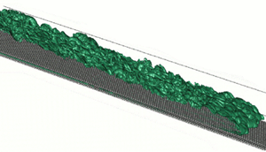
The  $c=0.1$ salinity contours shown in figure 3 demonstrate the spatio-temporal development of the flow for the representative simulation S3L15B, with
  $d_p=0.066$ and
  $Re_H = 10\ 355$. At
  $t/T_H =3.3$, the current displays coherent spanwise Kelvin–Helmholtz vortices, along with regular, small frontal lobes that move along the grooves between the top layer of spheres and hence reflect the periodicity of the bed arrangement. At
  $t/T_H=7.7$ these lobes remain nearly periodic, although their wavelength has doubled, while the tail is already fully three-dimensional. By
  $t/T_H=16.5$ the entire current has transitioned to a turbulent state.

Figure 3. The  $c=0.1$ salinity isosurface for simulation S3L15B at times
  $t/T_H=3.3$, 7.7 and 16.5. While the early stage of the current is dominated by coherent spanwise vortices, the flow transitions to a fully turbulent state later on.
Figure 4(a) displays the instantaneous salinity field in the plane  $z=0.4825$ for
  $t/T_H=17.6$, along with the projected velocity vectors. The current is seen to mix vigorously with the ambient fluid along the upper interface. The close-ups in (b,c) focus on the detailed flow features near the top of the particle bed, and indicate the numerical resolution of 40 grid cells per particle diameter, by showing the velocity vectors and salinity values at every grid point. The close-ups furthermore visualize the fluid exchange between the current and the bed, as dense current fluid leaks through the gaps between the spheres into the pore spaces. In addition, they show that the flow separates from the top of the spheres, which results in the strong deformation and folding of the fluid interface and thereby promotes mixing.

Figure 4. Concentration  $c$ (in blue) and velocity vectors in the plane
  $z=0.4825$, for simulation S3L15B at
  $t/T_H=17.6$. Panel (a) demonstrates that the current mixes vigorously with the ambient fluid along the upper interface, while it also exchanges fluid with the porous bed. The close-ups in (b,c), indicated by black rectangles in (a), highlight details of this current–bed interaction. Panel (b) shows every grid cell, so that it provides a measure of the spatial resolution.
Figure 5 displays the salinity concentration field averaged in the spanwise  $z$-direction over the fluid region only,
  $\langle c \rangle _{z}/ \langle \xi _f \rangle _z$, for simulation S3L15B at times
  $t/T_H=$ 7.7, 12.1 and 26.4. The current front propagating above the particle bed is qualitatively similar to that advancing over a flat bottom (Härtel et al. Reference Härtel, Meiburg and Necker2000). In addition, we observe a second front inside the porous bed that moves much more slowly, which is consistent with earlier experimental observations by Cenedese et al. (Reference Cenedese, Nokes and Hyatt2018). This second, slower front is driven by the dense fluid that leaks into the bed along the entire length of the current. The small difference between the salinity concentration values above and inside the bed in the lock region is due to numerical errors associated with the volume-of-fluid method, which cause a slight diffusive salinity flux into the particles.

Figure 5. Spanwise-averaged salinity  $\langle c \rangle _{z}/ \langle \xi _f \rangle _z$ in the head region of simulation S3L15B, at times
  $t/T_H$= 7.7 (a), 12.1 (b) and 26.4 (c). A conventional gravity current front propagates above the bed, while a second front advances more slowly inside the bed. With time, both the buoyant height
  $h$ (long–short dashed line) and the envelope
  $h_c$ (dashed line) of the current become more uniform along the length of the current.
During the early stages of the flow, the spanwise coherent Kelvin–Helmholtz vortices mentioned earlier mix the two fluids across nearly the entire free depth of the flow, cf. figure 5(a). Later on, after the flow has become fully three-dimensional and turbulent, the most intense mixing is restricted to a narrower region around the interface. Visual inspection of the  $c=0.1$ concentration isosurfaces at various intermediate times (not shown) indicates that the simulation with
  $Re_H=10\ 355$ (case S3L15C) transitions to turbulence somewhat earlier than the one for
  $Re_H=7486.2$ (case S1L15A), in line with our expectation that higher Reynolds numbers should promote more vigorous turbulence. We note that the dense current fluid quickly enters the spaces between the upper half of the top layer of spheres, as the resident light fluid in these exposed pores is easily carried away by the current. The infiltration of the current fluid into the lower layers of the sediment bed takes much longer, however, as the dense current fluid has to displace the lighter, resident fluid via a Rayleigh–Taylor-like instability in an effective porous medium. With time, both the buoyant height
  $h$ (long–short dashed line) and the current envelope
  $h_c$ (dashed line) tend to become more uniform along the length of the current, see figure 5(c) for
  $t/T_H=26.4$.
Figure 6 displays the salinity concentration field averaged in the spanwise  $z$-direction over the fluid region only,
  $\langle c \rangle _{z}/ \langle \xi _f \rangle _z$, for the experiment E3L15 at times
  $t/T_H= 7.7$, 12.1, and 26.4. The current front propagating above the particle bed is qualitatively similar to the simulations shown in figure 5. The simulations show a less uniform buoyant height and current envelope at earlier times because the experiments transitioned to a fully turbulent state at earlier times.

Figure 6. Spanwise-averaged salinity  $\langle c^+ \rangle _{z}$ in the head region for experiment E3L15, at times
  $t/T_H$= 7.7 (a), 12.1 (b) and 26.4 (c). Current propagates above bed similarly to the simulation counterparts in figure 5; however, with a more uniform buoyant height
  $h$ (long–short dashed line) and the envelope
  $h_c$ (dashed line).
Occasionally, it is preferable to analyse the flow in the reference frame moving with the front, with the front location at the origin of the coordinate system
 \begin{gather} c^+( {\boldsymbol{x} } - \boldsymbol{e}_x x_F(t ),t) = c ( {\boldsymbol{x}}, t ), \end{gather}
 \begin{gather}{\boldsymbol{u}}^+ ( {\boldsymbol{x}} - \boldsymbol{e}_x x_F(t) ,t ) = \boldsymbol{u} ( {\boldsymbol{x} } , t ) - v_F(t) \boldsymbol{e}_x . \end{gather}
We denote variables in this reference frame by a  $^+$-superscript. Figure 7 shows the spanwise-averaged concentration
  $\langle c^+ \rangle _{z}$ for experiment 3L15 at two different times. In addition to averaging in the spanwise direction, which is inherent to the LA method, we average the distribution around the given times by
  $\pm 1 T_H$ in order to smooth out fluctuations. For comparison, we display the corresponding simulation results for
  $t/T_H=22$ in (c).

Figure 7. Spanwise-averaged salinity  $\langle c \rangle _{z}$ in the head region for experiment E3L15, at times
  $t/T_H=5.3$ (a) and 22 (b). The panels also include the buoyant height
  $h$ (long–short dashed line) and the current envelope
  $h_c$ (dashed line). Corresponding simulation results for
  $t/T_H= 22$, shown in (c), are seen to agree closely with the experimental values. All distributions are averaged around the given time for
  $\pm 1 T_H$.
We note that the early experimental salinity field at  $t/T_H=5.3$ does not indicate the presence of the strong, spanwise coherent Kelvin–Helmholtz vortices that we had observed during the initial simulation stages of the simulation, cf. figure 5(a). This is likely a result of the much stronger initial perturbation introduced in the experiment by the removal of the gate, which causes the flow to transition to a fully three-dimensional turbulent state more rapidly than in the simulation. Nevertheless, by
  $t/T_H=22$ the experimental and computational concentration fields agree closely, especially with regard to the buoyant height as a function of the streamwise coordinate.
3.3. Front position and velocity
A key question concerns the influence of the porous bed on the front velocity of the current. Figure 8 presents experimental results for the non-dimensional front location  $(x_F -x_0)/H$ as function of time, where the value of zero corresponds to the front being at the position of the lock. While (a) shows values for the single-layer flows and the flat bottom, (b) provides corresponding data for the three-layer flows. The two-layer case behaves qualitatively similar, so that it is not shown. Within each panel the water depth
  $\tilde L_y$ is varied in order to assess its influence. Table 1 lists all experimental parameters.

Figure 8. Front location and velocity as functions of time, for the experiments listed in table 1. The left (right) column shows results for a single layer (three layers) of spheres. The upper (lower) row presents the front locations (front velocities) in free depth scales.
The experimental time  $\tilde t$ was normalized with the free depth time
  $\mathcal {T}_H$, and the front position with the free depth
  $\tilde H$. The time
  $\tilde t=0$ corresponds to the moment when the lock is opened. For a constant number of layers, this scaling causes the curves for the front locations to collapse approximately, although the shallower cases still propagate somewhat more slowly even when scaled with these free depth units, reflecting their effectively lower Reynolds numbers. In particular, we note that the current advancing over a smooth bottom travels only a few percentage points faster than the one propagating over a single layer of spheres. This indicates that during the early stages of the flow, the bottom roughness and the loss of current fluid into the porous bed of a single layer of spheres do not significantly retard the current.
Differentiation of the location values in (a,b) yields the front velocities, shown in (c,d), normalized with  $\mathcal {U}_H$, as a function of time. For all water depths the front velocity
  $\tilde v_F/ \mathcal {U}_H$ decreases with time, although this trend is most pronounced for the shallow water depths, which indicates that over time the bed roughness and porosity have a relatively larger influence on shallower currents.
Very prominent features of the front velocity data are their strong oscillations in time, which to the best of our knowledge had not been reported in earlier laboratory experiments. We hypothesize that these front velocity oscillations are caused by the presence of seiche waves generated by the removal of the lock gate. In order to test this hypothesis, let us consider the first seiche mode in a channel, which has a wavelength  $\lambda$ of twice the channel length. For our experiments this wavelength is large compared to the water depth, so that we can consider the seiche a shallow, linear wave with a phase speed
  $\tilde c_w = \sqrt {g\tilde H}$. The period
  $\tilde T_w$ of the wave, and the maximum speed
  $\tilde u_w$ of a fluid particle beneath the surface are given by
 \begin{gather} \tilde T_w = \frac{\tilde \lambda}{\tilde c_w} = \frac{2 \tilde L_x}{\sqrt{g\tilde H}}, \end{gather}
 \begin{gather}\tilde u_w = \frac{g \tilde \chi_w}{\tilde c_w} = \frac{g\tilde \chi_w}{\sqrt{g \tilde H}} , \end{gather}
where  $\tilde \chi _w$ denotes the maximum free surface deflection of the wave, which is small enough to be hardly visible in the experiment. For experiment E3L15 (
 $\tilde {H} = 0.126$ m and
  $L_x = 6.2$ m) (3.5) gives a period of
  $\tilde {T}=11.2$ s, or
  $\tilde {T}/\mathcal {T}_H = 7.4$. This value closely matches the oscillation period observed for E3L15 in figure 8. For the other experiments we found a similar level of agreement. For E3L15 the maximum velocity was 0.5 cm s
 $^{-1}$ greater than the mean. We employ this value as an estimate for the maximum velocity of a fluid particle beneath the surface in the absence of the current. Equation (3.6) then yields a maximum free surface deflection of 0.6 mm, which is small enough not to be noticed in most laboratory set-ups. In the following discussion, we assume that the seiche waves did not impact the mean current behaviour, beyond causing the current velocity to oscillate. We furthermore remark that the simulations do not generate seiche modes, as they assume a rigid upper surface.
Figure 8(c,d) includes linear fits to the front velocity data over the entire time  $\tilde T_{exp}$ of the experiments in order to better visualize the trends in the data. We fit (by means of minimizing the squared error
  $\epsilon ^2$) the slope
  $\alpha$ to the experimental data, which formally reads as
 \begin{equation} \tilde v_F / \mathcal{U}_H = \langle \tilde v_F \rangle_t/\mathcal{U}_H+ \alpha (\tilde t - \tilde T_{exp}/2 -\tilde t_0)/\mathcal{T}_H + \epsilon.\end{equation}
In (3.7), the average front velocity is obtained as  $\langle \tilde v_F \rangle _t = (\tilde x_F(\tilde T_{exp})- \tilde x_F(\tilde t_0)) / \tilde T_{exp}$, where
  $\tilde t_0$ is the time when the front is detected initially. Moreover, we define the densimetric Froude number
 \begin{equation} Fr(t)=\tilde v_F(t) / \mathcal{U}_H. \end{equation}
Column 9 of table 1 provides the average dimensionless front speeds. For most experiments the front velocity decreases with time, although for the deeper cases with only one particle layer, we observe a small increase during the analysed time interval. In general, the currents slow down more rapidly for larger relative bed heights  $\tilde \eta / \tilde H$.
We perform a corresponding fit for the simulations, although there we exclude the initial laminar phase of the flow. The time interval  $t\in \tau =[\tau _0, \tau _1]$ over which we evaluate the linear fit is given in table 3. In order to conduct meaningful comparisons, we evaluate the linear fit (3.7) at identical times
  $t/T_H=20$ for all experiments and simulations, to obtain
  $Fr|_{t/T_H=20}$. When plotting
  $Fr|_{t/T_H=20}$ against
  $d_p/H$, see figure 9, with error bars included based on the range of repeat experiments, we find that the Froude number is primarily a function of the relative particle size
  $d_p/H$, whereas the number of layers generally plays only a secondary role. An obvious exception to this rule is the single-layer case (square symbol) for large
  $d_p/H$, which differs substantially from the two- and three-layer cases with a similar
  $d_p/H$ (star and diamond symbol), in line with the observations reported in § 3.4.

Figure 9. Experimental and numerical results showing the correlation between sphere diameter  $d_p/H$ and Froude number evaluated at
  $t/T_H=20$,
  $Fr|_{t/T_H=20}$. Different symbol shapes represent different numbers of layers, with red (black) symbols representing experiments (simulations). Error bars for experiments are based on the range of repeat experiments. Simulations for constant
  $d_p/H$ but changing Reynolds and Schmidt numbers are included. The precise parameter values can be found in table 3 (simulations) and table 1 (experiments). As a general trend, the front velocity decreases with increasing particle size, whereas the number of layers plays a secondary role.
Cenedese et al. (Reference Cenedese, Nokes and Hyatt2018) carried out lock-exchange experiments with similar depths to those in the experiments reported here. They found Froude numbers similar to ours for currents propagating over smooth beds. These are also similar to other experimental studies of gravity currents over smooth beds (Simpson Reference Simpson1999; Shin et al. Reference Shin, Dalziel and Linden2004; Cantero et al. Reference Cantero, Balachandar and Garcia2007). Cenedese et al. (Reference Cenedese, Nokes and Hyatt2018) also carried out experiments with staggered beds of vertically arranged circular cylinders and when these were densely distributed the currents propagated atop the roughness. With cylinder heights of 10 mm, the same roughness height as our experiments with 1 layer of particles, they observed Froude numbers consistently lower than ours. We explain this by their experiments having a larger and more unobstructed volume of fluid within the bed such that the vertical exchange of fluid between the bed and the current head was larger than in our experiments.
Figure 10(a) displays the front velocities of experiment E3L15 and the corresponding simulation S3L15C as functions of time.

Figure 10. Comparison of experimental and numerical results for the front velocities/ densimetric Froude numbers. In (a) the evolution for experiment E3L15 is compared to different simulations showing a close fit between the experiment and simulations. Panel (b) compares experiments E0L20, E3L20, E1L15, E3L15 and E3L10 with simulations S0L15B, S3L20A, S3L15B and S3L10A in terms of time-averaged densimetric Froude numbers  $\langle v_F/ U_H \rangle _{\tau _{over}}$, where cases are categorized by the non-dimensional particle diameters
  $d_p/H$. For the exact values, see table 4. These show experiments to generally have a larger front speed than the simulations with this difference being more prominent when
  $d_p/H$ is small.
Table 4. Experimental and simulation values of front velocities and averaged buoyant heights. The averages are taken over  $\tau _{over}$, which is the time interval for which we have both experimental and simulation data in figures 10 and 12, respectively.

 $^{a}$Simulation S0L15A was carried out with no-slip boundaries at
  $z=0, L_z$.
 $^{b}$Simulations S0L15C and S3L15C were performed with
  $Sc=1$, as compared to the standard value of
  $Sc=7$.
The experimental data again show the pronounced seiche oscillations, while the simulation results exhibit somewhat smaller, more random-like variations. Nevertheless, experimental and numerical front velocities are seen to fluctuate around comparable mean values, and they show similar rates of decline. For a quantitative comparison, we average the experimental and computational front velocities over the time interval  $\tau _{over}$ from
  $2 < t/T_H < 28$, in order to obtain
  $\langle v_F/ U_H \rangle _{\tau _{over}}$ shown in figure 10(b). The experimental front velocities are generally slightly higher than the computational values. This difference tends to increase as
  $d_p/H$ decreases, such that the difference is largest for the smooth case. We need to keep in mind, however, that for the smooth case the experimental Reynolds number was about twice that of the corresponding simulation, which may account for much of this difference.
In order to assess the influence of  $Re$ and
  $Sc$ on the front velocity, we carried out two additional simulations for the smooth case. While S0L15B uses the standard set-up, S0L15A employs no-slip sidewalls, and S0L15C has a reduced Schmidt number value of
  $Sc=1$. We found that the lower
  $Sc$-value slightly reduced the front velocity, while the no-slip sidewall affected the front velocity by much less than one per cent.
3.4. Current height
The velocity of a gravity current, along with its destructive potential, are largely functions of the buoyant height. This height, in turn, depends on the net exchange of fluid between the frontal region and the tail section of the current, as well as on the leakage of current fluid into the porous bed. In this section, we will present results for the buoyant height of the current front as a function of time, and subsequently analyse the respective fluid exchange of the front with the tail section and the bed.
Let us consider the average height  $h_M$ of a current within a distance
  $4H$ behind the front. Figure 11 presents experimental results for
  $h_M/H$ as a function of time for different parameter combinations. While all experiments show a decline of
  $h_M/H$ with time, the rate of this decline depends on the specific experimental conditions. Panel (a) demonstrates that, when the number of sphere layers is held constant at three, the buoyant height decreases more slowly in deeper water, i.e. for a larger ratio of buoyant height to bed height,
  $h_M/\eta$. In (b), we recognize that, in deep water, one, two and three layers of spheres result in approximately identical buoyant heights with similar rates of decline. However, this rate of decline is significantly larger than for a current over a flat bottom (E0L20, orange line).

Figure 11. The spatially averaged current height  $h_M$ as a function of time for four groups of experiments: (a) constant number of particle layers, but varying water depth; (b) constant water depth, but different numbers of layers; (c) water depth of 15 cm, varying number of layers; and (d) water depth of 10 cm, varying number of layers.
Panels (c,d) suggest that, for shallower total water depth, the difference between currents propagating over one, two or three layers increases. Taken together, these observations indicate that currents over porous beds behave in a fundamentally different way from those over flat beds, and that the exact depth of the porous bed becomes influential only in relatively shallow water. This suggests that a thick current traveling in deep water moves so fast that only fluid from the uppermost pores gets mixed into the current front. Shallower currents that travel more slowly, on the other hand, are more likely to allow fluid from the lower pores to rise and become mixed into the current front. The fluid exchange between the current and the bed will be analysed in more detail below.
Figure 12 compares the buoyant front height  $h_M$ for the simulations to the corresponding experimental values. The time-averaged values
  $\langle h_M \rangle _{\tau _{over}}$ are provided in table 4. We note that, early on, the simulations tend to have larger buoyant front heights than the corresponding experiments, whereas the agreement improves at later times. This may at least partially be due to the perturbations introduced in the experiments by the removal of the gate and by the step in the sediment bed height, which are likely to promote an earlier transition to a fully turbulent state. Furthermore, the current height is seen to decrease for larger Reynolds number in the shallow simulations, which may again reflect the earlier transition to turbulence, cf. simulations S3L10A and S3L10B in figure 12(c). Finally, (d) shows that for smooth currents a lower Schmidt number is associated with a decrease in
  $h_M/H$, while for rough beds panel (b) shows no significant difference between the simulations for
  $Sc=7$ and
  $Sc=1$.

Figure 12. Comparison of experimental and numerical results for the front height  $h_M$. The agreement generally improves with time, which suggests that the discrepancy is mainly due to differences in the initialization of the currents.
The decrease in  $h_M$ indicates that the current head loses salinity either into the bed or into the tail section of the current. This issue will be discussed in more detail below. In order to further analyse the dilution of the current front, we calculate the height
  $h_r$ as the maximum
  $y$-value where
  $\langle c\rangle _z=0.1$, at the fixed streamwise location
  $x=-2H$ relative to the front location of the current. Figure 13(a) shows that for the three-layer experiments and the smooth bottom case, respectively,
  $h_r$ decreases with time. Figure 13(b) indicates that
  $h_M$ decreases even more rapidly than
  $h_r$, so that the currents not only see a reduced height, but also become more dilute.

Figure 13. Experimental measurements for  $h_r/H$ (a), and
  $h_M/h_r$ (b) indicate that as their height decreases, the currents also become more dilute.
3.5. Streamwise velocity profiles
Figure 14 compares the streamwise velocity profiles for experiments and simulations of gravity currents over a smooth wall, as well as over one or three layers of spherical particles. The velocity profiles are evaluated at a distance  $2H$ behind the front, and they are averaged both in the spanwise direction and over the time interval
  $13 \le t/T_H \le 15$. The peak velocities in both simulations and experiments are somewhat larger for the smooth wall, suggesting that rough sediment beds enhance the vertical mixing of streamwise momentum. Near the smooth wall, the velocity is smaller than near the surface of the sediment beds, which indicates that gravity currents propagating over rough beds see a small effective slip velocity at the bed surface. The above velocity profiles are similar to those observed by Zhou et al. (Reference Zhou, Cenedese, Williams, Ball, Venayagamoorthy and Nokes2017) in what the authors refer to as the overflowing regime.

Figure 14. Streamwise velocity profiles, averaged in the spanwise direction, for zero, one and three layers of spheres. The profiles are evaluated at location  $x= x_F-2H$, and they are averaged over the time interval
  $13 \le t/T_H \le 15$. When employing the PTV technique, the velocity values within approximately
  $3$ mm of the bottom and the top of the flume are affected by reflections, so that we do not show any experimental data in those regions.
4. Analysis of mass and momentum transfer
4.1. Mass transfer
The experimental and simulation results presented in the preceding section show several interesting findings regarding the influence of the porous particle bed on the overall gravity current properties. Among them are the exchange of fluid between the current and the bed, a somewhat reduced front velocity that depends mostly on the particle size, a more rapid decrease of the current height and front velocity with time, and a modified velocity profile within the current due to enhanced vertical mixing of streamwise momentum. In order to obtain more detailed insight into the mechanisms by which the particle bed effects these changes, we now proceed to analyse the mass and momentum transfer between the current and the bed in depth.
We begin by analysing the transport of salinity into and out of the current head, in the reference frame moving with the front. Towards this end, we focus on the control volume  $M(t)=[x_F(t)-x_{ML}, x_F(t)+ x_{MR}] \times [\eta , L_y] \times [0, L_z]$, with
  $x_{ML}=4H$ and
  $x_{MR}=0.5H$. Integrating transport equation (2.12) over this volume and dividing by its size
  $V_M= M_x H L_z$, where
  $M_x=x_{ML}+x_{MR}= 4.5H$, yields
 \begin{equation} \partial_t \frac{1}{V_M} \int_M c \, \textrm{d}V = \frac{1}{V_M} \int_{\partial M} \left [ v_F c \boldsymbol{e}_x - \boldsymbol{u} c + Pe_L^{-1} \boldsymbol{\nabla} c \right ]\boldsymbol{\cdot} \boldsymbol{n} \, \textrm{d}A ,\end{equation}
with  $\boldsymbol {n}$ representing the outward normal to the boundary
  $\partial M$ of control volume
  $M$. By introducing the streamwise velocity in the moving reference frame
  $u_x^+= u_x-v_F$ and neglecting the small contributions due to diffusion, we obtain
 \begin{equation} \partial_t \langle c \rangle_M = \langle u_x^+ c^+ \rangle_{\partial M, W }\frac{1}{M_x} + \langle u_y^+ c^+ \rangle_{\partial M, S }\frac{1}{H}.\end{equation}
Here, the volume average over  $M$ is denoted by
  $\langle \rangle _M$, while
  $\langle \rangle _{ \partial M, W}$ and
  $\langle \rangle _{ \partial M, S}$ indicate the surface averages of the fluxes across the western and southern boundaries, used to define the boundaries at
  $x^+ = -4H$ and
  $y=\eta$, respectively.
Figure 15 presents the temporal variation of the terms in the mass balance equation (4.2), for one flow over a smooth wall and three flows over three particle layers of different size. We observe that over time all current heads lose salinity, although the loss rate tends to decrease with time for all flows except the one with the largest particles. The relatively large temporal fluctuations in the rate of loss to the current tail may be related to vortical structures as well as variations in the interface height. Interestingly, the loss of current fluid into the bed increases with particle size  $d_p/H$, whereas the loss of salinity to the tail (blue dashed-dotted line) decreases. The reasons behind this influence of the particle size will be discussed below.

Figure 15. Mass balance terms according to (4.2), averaged over a moving window of two time units. The loss of current fluid into the bed (green line) increases with particle size, while the loss of head fluid to the tail (blue dash-dotted line) decreases for larger particles.  $(a)\ \textrm{S0L15B}, d_{p}/ H = 0; (b)\ \textrm{S3L20A}, d_{p}/H = 0.056; (c)\ \textrm{S3L15B}, d_{p}/H = 0.081; (d)\ \textrm{S3L10B}, d_{p}/H = 0.14.$
Figure 16 presents simulation results in the moving reference frame for the averaged salinity flux  $\langle c^+ u_x^+\rangle _{z,\tau }$ across the western boundary at
  $x^+ = -4H$. The profiles shown are averaged over a time interval
  $\tau =[\tau _0, \tau _1]$ that excludes the initial laminar evolution, with the specific time values provided in table 3. Compared to the flow over a smooth wall, the flows with particle layers exhibit lower salinity fluxes from the head into the tail just above
  $y = \eta$, and from the tail into the head further away from the lower boundary. This observation is consistent with the velocity profiles shown in figure 14, and it reflects the influence of the effective slip velocity at
  $y = \eta$ mentioned earlier for the flows over particle beds, along with increased vertical mixing in those flows. We will further explore the vertical mixing of momentum in § 4.2.

Figure 16. Streamwise salinity flux in the moving reference frame  $\langle u_x^+c^+ \rangle _{z,\tau }$ across the western boundary at
  $x^+=-4H$ as a function of the vertical coordinate, shown on a log scale. Compared to a flow over a smooth wall, the flows with particle beds exhibit reduced salinity fluxes from the head into the tail near the lower boundary, and from the tail into the head further away from the boundary.
Figure 17 analyses the time-averaged salinity flux from the current head into the bed, again in the moving reference frame. At the level of the bed surface,  $y = \eta$, (a) shows that this flux has a pronounced maximum over the interval
  $0>x^+/H>-1$, while it levels off thereafter. This indicates that the current front is very effective at sweeping the ambient fluid out of the primary pore spaces and replacing it with current fluid. Here we define the primary pore spaces as the exposed pore spaces between the upper halves of the topmost layer of spheres. Larger particle sizes are associated with a larger primary pore space volume, and thus result in an increased vertical flux. The high-frequency oscillations reflect the periodicity of the bed arrangement.

Figure 17. Time-averaged vertical salinity flux from the current head into the bed. (a) Flux at the top of the bed,  $y = \eta$, and (b) flux at the centre of the first particle layer,
  $y= \eta - d_p/2$. The different lines correspond to simulations S3L20A, S3L15B, S3L10B, S3L10C and S1L15A (top to bottom of the legend). The brown short–long dashed line corresponds to a single layer of particles, whereas all other simulations have three layers. The small salinity flux into the bed for
  $x>0$ results from our definition of the front as the location where the current height
  $h=0.1$, so that the current extends slightly beyond
  $x=0$.
The subsequent transport of current fluid into the deeper pore layers occurs more slowly. This is demonstrated by figure 17(b), which shows that the vertical flux at the centre of the first particle layer,  $y= \eta - d_p/2$, ramps up only gradually behind the current front. A comparison of (a,b) indicate that for
  $x/H < -1$ this flux into the deeper pore spaces roughly equals the flux at the bed surface, which suggests that by then the ambient fluid has largely been removed from the primary pore volume. The effective permeability of the bed increases with the particle size, which explains the enhanced salinity flux into the deeper layers of the bed for larger particles, as seen in (b). Interestingly, the
  $Re_H = 11\ 000$ simulation (beige solid line) transports more salinity into the bed than the
  $Re_H = 8000$ one, which may reflect the mobility increase due to the lower viscosity resistance. The single-layer simulation (brown line) shows a reduced flux due to a lower volume of bed fluid that can be exchanged, as compared to an equivalent three-layer simulation (green line).
From geometric considerations, it follows that the primary pore space volume  $V_{inter}$ per
  $x,z$-base area
  $A$ is
 \begin{equation} V_{inter}/A=K_{inter}d_p, \quad\text{where } K_{inter}= \frac{\sqrt{3} - {\rm \pi}/3}{2\sqrt{3}}=0.1977 , \end{equation}
so that the current front overruns primary pore space volume per unit width at the rate  $\langle v_F \rangle _{\tau } K_{inter}d_p$. Within the distance
  $H$ behind the front, current fluid enters the bed at the rate
  $\int _{-H}^{0} \langle u_y^+ c^+ \rangle _{z, \tau } \textrm {d}x$. Hence
 \begin{equation} \sigma= \frac{\int_{-H}^{0} \langle u_y^+ c^+ \rangle_{z, \tau} \textrm{d}x }{- \langle v_F \rangle_{\tau} K_{inter}d_p},\end{equation}
denotes the fraction of primary pore space fluid that is swept out within the distance  $H$ behind the front. Figure 18 indicates that
  $\sigma$ increases with the particle diameter, and typically lies in the range of
  $0.5\pm 0.1$. This confirms our earlier hypothesis that a significant fraction of the primary pore fluid gets flushed out within a distance
  $H$ behind the front.

Figure 18. Fraction  $\sigma$ of the primary pore space fluid that is flushed out by the current within a distance
  $H$ behind the front.
4.2. Momentum transfer
To analyse the momentum budget, we integrate the momentum balance
 \begin{equation} \partial_t \boldsymbol{u} + \boldsymbol{\nabla} \boldsymbol{\cdot} ( \boldsymbol{u} \boldsymbol{u})= -\boldsymbol{\nabla} p + Re^{-1} \boldsymbol{\nabla} \boldsymbol{\cdot} \left ( \boldsymbol{\nabla} \boldsymbol{u} + (\boldsymbol{\nabla} \boldsymbol{u})^T \right ) - \boldsymbol{e}_y c \end{equation}
over the moving control volume  $\hat M=[x_F-4H, x_F+ 0.5H ]\times [\eta , \eta +\zeta ]\times [ 0, L_z]$ and divide by the spanwise domain width
  $L_z$. Note that
  $\hat M$ does not cover the entire vertical extent of the domain, but only the region from the bed surface at
  $y=\eta$ to the distance
  $\zeta$ above the bed where the streamwise velocity in the moving reference frame vanishes. Hence
  $y= \eta + \zeta$ can be viewed as the boundary between the current and the ambient counterflow. Figure 19 displays the spanwise-averaged value of
  $\zeta$ at different times, relative to the front position. It shows that both for a smooth wall and a rough bed
  $\zeta /H$ fluctuates around the value of 0.3 in the tail, so that we pick
  $\zeta /H=0.3$ as the upper boundary of the control volume for the momentum balance.

Figure 19. Boundary between the current and the counterflow for evaluating the momentum balance, as defined in the text. (a) Flow simulation S0L15B over a smooth wall, and (b) flow simulation S3L20A over a bed of three particle layers.
In compact notation, we can write the  $x$-component of the integrated (4.5) as
 \begin{equation} \zeta M_x \partial_t \langle u_x \rangle_{ \hat M} =\zeta { \omega}_f + \zeta {\tau}_p + M_x {\tau}_h+ M_x{ \tau}_b , \end{equation}
where the individual terms on the right-hand side are defined as
 \begin{equation} \left.\begin{array}{c@{}} \omega_f(t) = \langle u_x u_x - v_F u_x \rangle_{\hat M, W} - \langle u_x u_x - v_F u_x \rangle_{\hat M, E} , \\ \tau_p(t)= \langle\, p \rangle_{\hat M, W} - \langle\, p\rangle_{\hat M, E} , \\ \tau_h(t)= -\langle u_y u_x \rangle_{\hat M, N} + \dfrac{1}{Re_L} \langle \partial_y u_x \rangle_{\hat M, N} , \\ \tau_b(t)= +\langle u_y u_x \rangle_{\hat M, S}- \dfrac{1}{Re_L} \langle \partial_y u_x \rangle_{\hat M, S} . \end{array}\right\} \end{equation}
The terms in (4.6) represent, from left to right, the time rate of change of  $x$-momentum within the control volume, the net convective momentum flux across the east and west boundaries (
 $\omega _f$), the net pressure stress (
 $\tau _p$), the momentum flux through the top boundary of the current at a distance
  $\zeta$ above the bed (
 $\tau _h$) and the bed stress (
 $\tau _b$) due to viscous stress and the convection of momentum. Note that we neglect the viscous stresses at the west and east boundaries, along with the
  $x$-derivative of the vertical velocity at the south and north boundaries, as these terms are small.
Figure 20 displays the terms of (4.6) for the representative simulation S3L10B. We observe that the bottom friction  $\tau _b$ represents the main stress retarding the current, with a smaller contribution coming from the top friction
  $\tau _h$. These retarding forces are largely balanced by the convective momentum inflow
  $\omega _f$ and the streamwise pressure drop
  $\tau _p$, although the current still experiences a slight overall net deceleration. A detailed comparison with results from other simulations (not shown) indicates that the relative magnitude of the terms is similar for all simulations, although the absolute values can vary significantly, as will now be discussed for the bottom friction term.

Figure 20. Contributions to the streamwise momentum balance in the control volume for simulation S3L10B, according to (4.6). The data have been smoothed by employing a moving average extending over two time units. The retarding influence of the bottom and top friction is largely balanced by the convective inflow of momentum and the streamwise pressure drop.
4.2.1. Bottom friction
In order to explore the dependence of the bottom friction on the particle size, we define the friction coefficient  $C_f$ as
 \begin{equation} C_f(x,z,t) = -\frac{u_y u_x - Re_L^{-1} \partial_y u_x}{v_F^2/2} \quad \text{for } y=\eta . \end{equation}
Here, we included the convective transport of momentum as well, because a potential simplified model of the bed might assume an impermeable surface at  $y=\eta$ and then
  $C_f$ could be used to represent the full momentum transport.
Time-averaged friction coefficient data (the averaging interval is given in table 3) are provided in figure 21. These demonstrate that the friction coefficient increases with the particle size. Even for the smallest particles, the bottom friction is substantially larger than for the smooth wall. Closer inspection of the results shows that most of this increase stems from the convective term  $\langle u_y u_x \rangle _{z,\tau }$, which increases significantly for the largest particles with
  $d_p=0.1$.

Figure 21. Time-averaged bottom friction coefficient  $\langle C_f \rangle _{z, \tau }$ according to definition (4.8), for simulations S0L15B, S3L20A, S3L15B, S3L10C and S1L15A (from top to bottom in the legend).
Figure 22(a) displays the mean vertical velocity at the top of the bed as a function of the streamwise coordinate for selected simulations. The figure demonstrates that ahead of the front fluid is ejected out of the bed, while it is pushed into the bed below the current head. Panel (b) shows the variance of the vertical velocity at  $y=\eta$ for the same set of simulations sharing the line style with (a). We find that its value increases with the particle size and the Reynolds number, as a result of the increased fluid mobility within the bed.

Figure 22. (a) Mean vertical velocity component at the top of the bed for five simulations of flows over particle beds (S3L20A, S3L15B, S1L15A, S3L10B, S3L10C) (from top to bottom in the legend). Fluid is ejected out of the bed ahead of the front, and into the bed below the gravity current head. (b) Variance of the vertical velocity. This quantity increases with the particle size and the Reynolds number, reflecting the increased mobility of the fluid within the bed.
Based on Darcy's law, we can estimate the magnitude of the vertical velocity  $u_D$ into the porous bed as
 \begin{equation} u_D \frac{\mu}{\tilde K}= \boldsymbol{\nabla} p, \end{equation}
where  $\tilde K$ denotes the permeability of the bed. Carman (Reference Carman1997) showed empirically for flow through glass spheres with a porosity
  $\phi _f$ that the permeability can be approximated by
 \begin{equation} \tilde K = \frac{d_p^2\phi_f^3}{180(1-\phi_f)^2}. \end{equation}
 For a densely packed bed with  $\phi _f = 0.26$ and
  $d_p=0.01$ m, this results in a permeability of
  $\tilde K = 1.8\times 10^{-8}$ m
 $^2$. For a current height of approximately half the depth and negligible dilution, we can write (4.9) as
 \begin{equation} u_D =\frac{\frac{1}{2}{\rm \Delta} \rho g \tilde{H} \tilde{K}}{\rho_1\tilde{H}\nu} = \frac{1}{2}\mathcal{U}_H\frac{\tilde K}{\tilde H^2}Re_H,\end{equation}
or
 \begin{equation} u_D/ \mathcal{U}_H = \frac{1}{2}\frac{\tilde K}{\tilde H^2}Re_H. \end{equation}
 We find that this predicts the correct order of magnitude for the downward velocities in figure 22(a). However, it significantly underpredicts the increasing velocities into the bed with increasing  $d_p$, and overpredicts the increase in velocity with Reynolds number. The imperfections in applying the Darcy model to the flow into the bed are not unexpected because of the shallow depth of the rough bed, the relatively large size of the grains, and the sidewalls adding complexity to the flow. Due to the large pore size a Darcy–Brinkman formulation may be more applicable to the problem. The empirical constants in such a model are less accurately predictable and the model would still experience imperfections due to the sidewalls and the shallow depth of the bed.
Based on classical investigations of turbulent flows over rough walls (Nikuradse Reference Nikuradse1931; Schlichting Reference Schlichting1936; Pope Reference Pope2000), we expect the bottom friction to depend on the ratio of the particle radius to the thickness of the viscous sublayer. In order to be able to estimate the latter, we introduce the friction velocity
 \begin{equation} u_\tau =\frac{\sqrt{ \nu \partial_{ \tilde y} \tilde u_x}} {\mathcal{U}_L }= \sqrt{\partial_y u_x/ Re_L } , \end{equation}
and a length scale  $L_W$ for the near-wall region
 \begin{equation} L_W = \frac{\nu}{\tilde u_\tau \tilde L_y} = (\partial_y u_x Re_L )^{-1/2} = u_\tau^{-1} Re_L^{-1}. \end{equation}
Figure 23(a) displays streamwise velocity profiles in wall units (solid line) at  $x-x_F= -2H$, for three different simulations. A comparison with the linear profiles
  $u_\tau y/L_W+ u_x(y=\eta ) / u_\tau$ (dashed line) demonstrates that the viscous sublayer extends to the typical value of five wall units, i.e.
  $y-\eta \approx 5L_w$. Panel (b) shows the mean friction coefficient as a function of the particle radius normalized by the wall unit
  $L_W$. All of the cases with particle layers are seen to fall into the transitional roughness regime
  $10<d_p/(2L_W)<30$, indicating that the particle radius is slightly to substantially larger than the viscous sublayer thickness. Interestingly, the friction coefficient strongly increases once the particle radius exceeds about twenty wall units, as a result of the increased advective momentum mixing seen earlier in figure 22. This observation is consistent with the work of Fang et al. (Reference Fang, Han, He and Dey2018) and Manes et al. (Reference Manes, Pokrajac, McEwan and Nikora2009), who investigated open channel pressure-driven flows over fixed beds of spheres, finding enhanced momentum mixing for larger bed permeabilities.

Figure 23. (a) Spanwise- and time-averaged streamwise velocity profiles, evaluated  $2H$ behind the front and scaled with wall units, cf. (4.13) and (4.14). Panel (b) shows the averaged friction coefficient, (4.8), as a function of the particle size scaled with the wall length
  $L_W$. The values of the wall lengths are
  $L_W=2.2\times 10^{-3}$,
  $2.2\times 10^{-3}$,
  $1.9 \times 10^{-3}$,
  $2.2\times 10^{-3}$,
  $1.8\times 10^{-3}$ and
  $2.0\times 10^{-3}$, respectively, for simulations S0L15B, S3L20A, S3L15B, S3L10B, S3L10C and S1L15A. Note that the friction coefficient increases significantly when the particle radius exceeds approximately twenty wall units.
5. Discussion and conclusion
We have presented a detailed experimental and computational study into gravity currents propagating over fixed beds of monodisperse spherical particles. The investigation provides insight into how the number of particle layers and the ratio of particle size to water depth affect the exchange of mass and momentum between the current and the bed, and hence the decay of current height and velocity with time.
We find that the mass exchange between the current and the bed involves two separate steps that operate on different time scales. In a first step, the dense current front rapidly sweeps away the resident fluid in the exposed pore spaces between the top layer of spheres. We develop a conceptually simple quantitative model for this process that compares well with experimental and simulation data. As a second step, a buoyancy-driven vertical exchange flow between the current and the deeper pores is set-up that takes significantly longer to develop. This process depends on the permeability of the bed, which in turn is a function of the particle diameter, and it plays an important role mostly for shallow currents that travel relatively slowly.
The momentum exchange between the current and the bed strongly depends on the particle size as well, and especially on its relative magnitude compared to the viscous sublayer of the current. The bottom friction is moderate when the particle size is smaller than or comparable to the thickness of the viscous sublayer, but it jumps for particles that strongly protrude from the sublayer, leading to a more rapid deceleration of the flow. At the same time, the number of particle layers is seen to affect the front velocity only weakly.
We note that the present lock-exchange experiments and simulations focused primarily on the early stages of the gravity current development. While we expect that the current/bed interaction gains in importance during the later stages of the flow, when the current becomes shallower and slows down as a result of viscous effects, current experimental and simulation resources did not allow us to address these late stages.
Acknowledgements
A.M. and R.N. would like to thank I. Shephard and K. Wines, P. Bruneau and P. Branje for their expertise and help with the experimental apparatus at the University of Canterbury. A.M. wishes to acknowledge the financial support provided to him through the University of Canterbury doctoral scholarship. E.M. gratefully acknowledges support from the National Science Foundation under grant CBET-1803380, from the Army Research Office under grant W911NF-18-1-0379 and through NEEC grant N00174-16-C-0013. T.K. acknowledges financial support by the Deutsche Forschungsgemeinschaft under grant KO5515/1-1. This work used the Extreme Science and Engineering Discovery Environment (XSEDE) Stampede 2 at the TACC through allocation TG-CTS150053. We would like to thank the three anonymous referees for their valuable comments, which significantly improved the final paper.


