2.1. Governing equations for interfacial two-phase flow

As the stability computations are facilitated using the same numerical methods as the nonlinear solver, a recapitulation of the discretisation and schemes used in this work is given here. From a physical viewpoint, it is assumed that both fluid phases are separated by an interface of negligible thickness. The molecular imbalance of cohesive forces between both fluids is modelled as a surface tension force, acting on the interface. The numerical representation of the phases and the interface can be either Lagrangian or Eulerian. Current nonlinear solvers usually use the level set method (Sussman, Smereka & Osher Reference Sussman, Smereka and Osher1994), the VOF (e.g. Scardovelli & Zaleski Reference Scardovelli and Zaleski1999) or methods derived thereof, all of which use an Eulerian representation, resulting in a non-conformal interface representation of finite thickness. The incompressible continuity and momentum equations, including variable density and surface tension, are given in unified form as

(2.1a)\begin{gather} \partial_t \rho + \boldsymbol{u} \boldsymbol{\cdot} \boldsymbol{\nabla} \rho = 0, \end{gather}

(2.1b)\begin{gather}\rho (\partial_t \boldsymbol{u} + \boldsymbol{u} \boldsymbol{\cdot} \boldsymbol{\nabla} \boldsymbol{u} ) ={-}\boldsymbol{\nabla} p + \boldsymbol{\nabla} \boldsymbol{\cdot} \left( \mu \boldsymbol{\mathsf{D}} \right) + \sigma \kappa \boldsymbol{n} \delta(\boldsymbol{x}-\boldsymbol{x_s}) \end{gather}

with $\boldsymbol {u} = (u,v,w)^{\textrm {T}}$ the velocity vector, $\rho$ the density, $\mu$ the dynamic viscosity, $p$ the pressure and $\boldsymbol {x_s}$ the position of the interface. The deformation tensor is $\boldsymbol{\mathsf{D}} = \boldsymbol {\nabla } \boldsymbol {u} + \boldsymbol {\nabla }^{\textrm {T}} \boldsymbol {u}$. Density and viscosity differ between the phases but are constant within each phase. The right-most term in (2.1b) represents the surface tension force along the interface, and is composed of the surface tension coefficient $\sigma$, the local interface curvature $\kappa$, the unit normal vector of the interface $\boldsymbol {n}$ and $\delta$, the Dirac $\delta$-function that is non-zero on the interface. Using a Heaviside function $H(\boldsymbol {x}-\boldsymbol {x_s})$, that is $1$ in phase $1$ and $0$ in phase $2$, $\rho$ and $\mu$ can be expressed as

(2.2a)\begin{gather} \rho = \rho_{2} + H(\rho_{1} - \rho_{2}), \end{gather}

(2.2b)\begin{gather}\mu = \mu_{2} + H(\mu_{1} - \mu_{2}). \end{gather}

2.2. Interface representations

Numerically, $H$ and $\delta$ are approximated as $H_\epsilon$ and $\delta _\epsilon$ where $\epsilon$ is a characteristic length scale related to the local grid size $\varDelta$. The method of computing the surface tension term is closely related to the immersed boundary method, introduced by Peskin (Reference Peskin1972) where we find a volumetric representation of the surface force as

(2.3)\begin{equation} \sigma \kappa \boldsymbol{n} \delta(\boldsymbol{x} - \boldsymbol{x_s}) = \sigma \kappa \boldsymbol{\nabla} H_\epsilon(\boldsymbol{x} - \boldsymbol{x_s}). \end{equation}

While several numerical representations of $H_\epsilon$ are possible, we will focus on two variants of the continuum surface force (CSF) method (Brackbill, Kothe & Zemach Reference Brackbill, Kothe and Zemach1992). In the CSF method, combined with the VOF method we set

(2.4)\begin{equation} H_\epsilon(\boldsymbol{x} - \boldsymbol{x_s}) = c(\boldsymbol{x}) = \begin{cases} 0, & \mathrm{for} \ \boldsymbol{x}\ \text{in phase 1}, \\ 1, & \mathrm{for} \ \boldsymbol{x}\ \text{in phase 2}, \\ 0.5, & \mathrm{for} \ \boldsymbol{x}\ \text{at the interface}, \end{cases} \end{equation}

where $c$ is the volume fraction field and $\epsilon = \varDelta$, the grid size. We then find $\boldsymbol {n} \delta = \boldsymbol {\nabla } c$. Similarly, when combining the CSF method with a level set method, we can find a smooth approximation

(2.5)\begin{equation} H_\epsilon(\boldsymbol{x} - \boldsymbol{x_s}) =H_\epsilon (\phi(\boldsymbol{x})) = \begin{cases} 0, & \mathrm{if}\ \phi <{-}\epsilon, \\ 1, & \mathrm{if}\ \phi > \epsilon, \\ \dfrac{1 + \phi/\epsilon + \sin({\rm \pi}\phi/\epsilon)/{\rm \pi}}{2}, & \mathrm{otherwise}, \end{cases} \end{equation}

where $\phi$ is usually chosen as a signed distance function with respect to the interface

(2.6)\begin{equation} \phi(\boldsymbol{x}) = \begin{cases} \phi > 0, & \mathrm{for}\ \boldsymbol{x}\ \text{in phase 1}, \\ \phi < 0, & \mathrm{for}\ \boldsymbol{x}\ \text{in phase 2}, \\ \phi = 0, & \mathrm{for}\ \boldsymbol{x}\ \text{at the interface}. \end{cases} \end{equation}

Here, we find $\boldsymbol {n} \delta = \boldsymbol {\nabla } \phi /|\boldsymbol {\nabla } \phi |\delta _\epsilon$ where the smooth delta function can be obtained as $\delta _\epsilon = \mathrm {d}H_\epsilon (\phi )/\mathrm {d}\phi$. Both methods usually lead to a characteristic interface thickness of $O(\varDelta )$ (Popinet Reference Popinet2018). Since $\rho$ is directly coupled to $c$ or $\phi$, respectively, (2.1a) is equivalent to the advection of $c$ or $\phi$

(2.7a)\begin{gather} \partial_t c + \boldsymbol{\nabla} \boldsymbol{\cdot} (c \boldsymbol{u})= 0, \end{gather}

(2.7b)\begin{gather}\partial_t \phi + \boldsymbol{\nabla} \boldsymbol{\cdot} (\phi \boldsymbol{u})= 0. \end{gather}

In Basilisk, the CSF method in combination with a VOF interface representation is used. However, for reasons described in § 3.3, we will adopt aspects of the level set method for the derivation and solution of the linearised code.

The discretisation of (2.3) warrants special attention as well-balanced schemes have to be used which are able to recover equilibrium solutions of certain continuous problems, thus avoiding the problem of so-called parasitic currents (Harvie, Davidson & Rudman Reference Harvie, Davidson and Rudman2006). An extensive discussion of this matter is given in Popinet (Reference Popinet2018). An essential requirement is that the same discrete operators are used for the gradients of the pressure $p$ and the Heaviside function $H_\epsilon$. The computation of the normals and curvature depends on the method used for the interface representation. Since for the level set method, $\phi$ is a continuous function, the curvature is easily computed as

(2.8a)\begin{gather} \boldsymbol{n} = \dfrac{\boldsymbol{\nabla} \phi}{|\boldsymbol{\nabla} \phi|}, \end{gather}

(2.8b)\begin{gather}\kappa = \boldsymbol{\nabla} \boldsymbol{\cdot}\boldsymbol{n}. \end{gather}

However, for the VOF–CSF method, direct derivation of $c$ leads to problematic curvature estimates because of its discontinuity. Therefore Basilisk, uses a height-function method that gives second-order accurate curvature estimates (Cummins, Francois & Kothe Reference Cummins, Francois and Kothe2005).

For illustration, in two dimensions a close-to-horizontal interface can be described by $y = h_y(x)$, where $h_y$ is the vertical distance to the interface at a given $x$. The normals and curvature of this interface are then computed as

(2.9a)\begin{gather} \boldsymbol{n} = \dfrac{(h_{y}',1)}{(1+h_y^2)^{1/2}}, \end{gather}

(2.9b)\begin{gather}\kappa = \dfrac{h_{y}''}{(1+h_y'^2)^{3/2}}. \end{gather}

For an interface $x = h_x(y)$ the procedure is similar. An extension to three dimensions is straightforward and described in Popinet (Reference Popinet2009).

2.3. Discretisation in Basilisk

The equation system (2.1) is discretised on regular Cartesian grids using a staggered-in-time discretisation, which is second-order accurate, yielding the following velocity and volume fraction update at every time step (Popinet Reference Popinet2003, Reference Popinet2009):

(2.10a)\begin{gather} \hspace{-4pc}\boldsymbol{u}^{n+1} = \boldsymbol{u}^{n} + \Delta t ( - \boldsymbol{u}^{n+1/2} \boldsymbol{\cdot} \boldsymbol{\nabla} \boldsymbol{u}^{n+1/2} - \boldsymbol{\nabla} p^{n+1}/\rho_{n+1/2}\nonumber\\ \hspace{4pc}+ \boldsymbol{\nabla} \boldsymbol{\cdot} [2 (\mu/\rho)_{n+1/2} (\boldsymbol{\mathsf{D}}_n + \boldsymbol{\mathsf{D}}_{n+1})] + [\sigma/\rho \kappa \boldsymbol{\nabla} c ]_{n+1/2}\vphantom{\boldsymbol{u}^{n+1/2}}), \end{gather}

(2.10b)\begin{gather} c^{n+1/2} = c^{n-1/2} - \Delta t \boldsymbol{\nabla} \boldsymbol{\cdot} (c^n \boldsymbol{u}^n ). \end{gather}

Pressure and velocity are decoupled using a standard time-splitting projection scheme (Chorin Reference Chorin1969). The advection term is computed using the Bell–Colella–Glaz (BCG) second-order unsplit upwind scheme (Bell, Colella & Glaz Reference Bell, Colella and Glaz1989), as will be described in § 3.2. A geometric VOF method is used to advect the volume fraction in (2.7a). The advection of a level set function $\phi$ is equivalent to the advection of a passive scalar which is advected using

(2.11)\begin{equation} \phi^{n+1/2} = \phi^{n-1/2} - \Delta t ~ \boldsymbol{\nabla} \boldsymbol{\cdot} (\phi^n \boldsymbol{u}^n ). \end{equation}

3.1. Derivation of the linearised equations

In order to obtain the linearised equations, we first non-dimensionalise the nonlinear equations (2.1b) with respect to $\rho _1$, $\mu _1$ and a suitable reference length and velocity scale, thus obtaining

(3.1)\begin{align} &[\tilde{\rho} + H_\epsilon(\phi) (1 - \tilde{\rho})] (\partial_t \boldsymbol{u} + \boldsymbol{u} \boldsymbol{\cdot} \boldsymbol{\nabla} \boldsymbol{u} )\nonumber\\ &\quad ={-}\boldsymbol{\nabla} p + \dfrac{1}{Re}\boldsymbol{\nabla} \boldsymbol{\cdot} [ (\tilde{\mu} + H_\epsilon(\phi) (1 - \tilde{\mu})) (\boldsymbol{\nabla} \boldsymbol{u} + \boldsymbol{\nabla}^{\textrm{T}} \boldsymbol{u}) ] + \dfrac{1}{We} \kappa \boldsymbol{n} \delta_\epsilon(\phi), \end{align}

where we have used the level set methodology to account for the two phases. The Reynolds number is $Re = \rho _1 U_{{ref}} D_{{ref}} /\mu _1$, the Weber number is $We = \rho _1 U^2_{{ref}} D_{{ref}} /\sigma$, $\tilde {\rho } = \rho _2/\rho _1$ and $\tilde {\mu } = \mu _2/\mu _1$. Note that, from (3.1) onward, all quantities are assumed to be dimensionless.

Starting point for the assessment of linear stability is the decomposition of the flow into a basic state and an infinitesimal perturbation, $\boldsymbol {u} = \boldsymbol {U} + \zeta \boldsymbol {u'}$ and $p = P + \zeta p'$ for the velocity and pressure respectively, with $\zeta \ll 1$. A similar linearisation is done for the level set function $\phi = \varPhi + \zeta \phi '$. Therewith associated are a perturbed curvature $\kappa = K +\zeta \kappa '$ and a normal vector $\boldsymbol {n} = \boldsymbol {N} +\zeta \boldsymbol {n}'$. We also make use of the base flow volume fraction $C$ but, as will be described in § 3.3, the use of a perturbation volume fraction poses several challenges and is thus avoided.

We insert the respective decompositions into ((3.1), (2.7b)) and retain only leading-order terms in $\zeta$. Dropping $\zeta$ for convenience, we arrive at

(3.2a)\begin{gather} [\tilde{\rho} + H_\epsilon(\varPhi) (1 - \tilde{\rho})] (\partial_t \boldsymbol{u'} + \boldsymbol{u'} \boldsymbol{\cdot} \boldsymbol{\nabla} \boldsymbol{U} + \boldsymbol{U} \boldsymbol{\cdot} \boldsymbol{\nabla} \boldsymbol{u'} ) + 2[\delta_\epsilon(\varPhi)\phi'(1-\tilde{\rho})](\boldsymbol{U} \boldsymbol{\cdot} \boldsymbol{\nabla} \boldsymbol{U}) \nonumber\\ \hspace{-6.5pc} ={-}\boldsymbol{\nabla} p' + \dfrac{1}{Re} \boldsymbol{\nabla} \boldsymbol{\cdot} [ (\tilde{\mu} + H_\epsilon(\varPhi) (1 - \tilde{\mu})) ( \boldsymbol{\nabla} \boldsymbol{u'} + \boldsymbol{\nabla}^{\textrm{T}} \boldsymbol{u'} ) ]\nonumber\\ \hspace{-2.2pc} + \dfrac{1}{Re} \boldsymbol{\nabla} \boldsymbol{\cdot} [ (\delta_\epsilon(\varPhi)\phi'(1-\tilde{\mu}) ( \boldsymbol{\nabla} \boldsymbol{U} + \boldsymbol{\nabla}^{\textrm{T}} \boldsymbol{U} )] + \boldsymbol{F}_{s}(\varPhi,\phi'), \end{gather}

(3.2b)\begin{gather}\partial_t \phi' + \boldsymbol{\nabla} \boldsymbol{\cdot} (\varPhi \boldsymbol{u'}) + \boldsymbol{\nabla} \boldsymbol{\cdot} (\phi' \boldsymbol{U}) = 0, \end{gather}

where we have used the fact that $\delta _\epsilon (\varPhi )$ is obtained as the distributional derivative of $H_\epsilon (\varPhi )$, during linearisation of terms involving $H_\epsilon (\phi )$. We further note that, as described in § 2.2, $H_\epsilon (\varPhi )$ can be replaced by $C$. Thereby, we retain an interface thickness of $O(\varDelta )$. Due to the involvement of two immiscible phases, the linearised equations contain a number of additional terms, compared to the linearised incompressible equations of a single fluid phase: the transport of the perturbation velocity by the base flow velocity and vice versa is scaled by the base flow density field. Additionally, a new advective term, composed only of the base flow velocity, appears that is acted upon by the perturbation density field. When comparing to a usual multi-domain approach of Navier–Stokes or Orr–Sommerfeld equations, where the interface height appears as a variable, this term corresponds to multiplication of the same base flow terms with a perturbation of the interface height. Similarly, a scaling of the perturbation velocity diffusion by the base flow viscosity field is introduced and a new term, representing the action of the perturbation viscosity field on the base flow velocity diffusion, appears.

The linearised surface tension force is given as

(3.3)\begin{equation} \boldsymbol{F}_{s}(\varPhi,\phi') = \dfrac{1}{We} [ \kappa' \boldsymbol{N}\delta_\epsilon(\varPhi) + K \boldsymbol{n}'\delta_\epsilon(\varPhi) + K \boldsymbol{N}\phi' \partial_\varPhi \delta_\epsilon(\varPhi)], \end{equation}

where $\partial _\varPhi$ in the right-most term denotes the functional derivative with respect to $\varPhi$, and $f(\partial _\varPhi \delta _\epsilon (\varPhi )) = (\partial _\varPhi f) \delta _\epsilon (\varPhi )$ for some test function $f$. As long as $\varPhi$ has signed distance, we can make use of the fact that, at the interface, any change of $\varPhi$ is along the normal $\boldsymbol {N}$, such that $\partial _{\boldsymbol {N}}\varPhi = 1$. Hence, we have

(3.4)\begin{equation} \partial_\varPhi (K\boldsymbol{N}\phi') \delta_\epsilon(\varPhi) =\partial_{\boldsymbol{N}} (K\boldsymbol{N}\phi')(\partial_{\boldsymbol{\varPhi}}\boldsymbol{N}) \delta_\epsilon(\varPhi) =\partial_{\boldsymbol{N}} (K\boldsymbol{N}\phi')\delta_\epsilon(\varPhi). \end{equation}

Consequently, we can write

(3.5)\begin{equation} K \boldsymbol{N}\phi' \partial_\varPhi \delta_\epsilon(\varPhi) = \boldsymbol{N} \boldsymbol{\cdot} \boldsymbol{\nabla} (K \boldsymbol{N}\phi') \delta_\epsilon(\varPhi). \end{equation}

The three terms representing the linearised surface tension force account for the action of the perturbation curvature on the basic state normal at the unperturbed interface and vice versa, as well as the action of the perturbed interface on the basic state curvature and normal. Similar terms can be identified in the linearised multi-domain formulation, there multiplied with the perturbation of the interface height (see Tammisola et al. Reference Tammisola, Lundell and Söderberg2012).

3.2. Implementation of linearised advection and diffusion terms

The computation of the linearised advection terms is facilitated using a slightly modified version of the numerical scheme that is used for the nonlinear advection in Basilisk. Here, we give a general overview of the scheme and necessary modifications. For the calculation of the nonlinear advection term $\boldsymbol {u}^{n+1/2} \boldsymbol {\cdot } \boldsymbol {\nabla } \boldsymbol {u}^{n+1/2}$ in (2.10a), a prediction of the velocity on the cell faces $\boldsymbol {u}_f^{n+1/2}$ is computed with a variant of the BCG scheme (Bell et al. Reference Bell, Colella and Glaz1989), using the pressure gradient and body forces at $t = n$. Solenoidality of the predicted velocity is enforced in a projection step. The advection step itself is performed by an isolated function which takes two arguments, a scalar field, in this case the cell centred velocity field $\boldsymbol {u}^{n}$, as well as $\boldsymbol {u}_f^{n+1/2}$, to compute the advection fluxes of $\boldsymbol {u}$.

For the linearised advection step, a prediction of the basic state velocity is not needed, since it is either stationary or known at all time steps (in case of a time-periodic base flow). Thus, the two linear advection terms can be computed by calling the advection routine twice, using $\boldsymbol {u'}^{n}$ and $\boldsymbol {U}_f^{n+1}$, or $\boldsymbol {U}^{n+1}$ and $\boldsymbol {u'}_f^{n+1/2}$. A small technicality is involved when advecting $\boldsymbol {U}^{n+1}$. The advection routine is implemented so that it by default adds the action of the advection to the tracer fields that are advected, i.e. $\boldsymbol {U}^{n+1}$. However, for both advection terms, the action needs to be added to $\boldsymbol {u'}^{n}$. To ensure this, minor modifications of the routine are necessary.

The second advection term, stemming from the density variation between the fluids, is computed again using the same BCG scheme. The diffusion term is added explicitly, as it only contains the basic state velocity.

3.3. Implementation of linearised interface advection

An adaptation of Basilisk's geometric VOF scheme for linear perturbation analysis is not straightforward. A naive linearisation of the volume fraction transport equation and the associated interface fluxes, as well as the geometric interface reconstructions would retain the scheme's inherent property of computing finite amplitude waves. The reason is rooted in the way the interface location is defined in VOF methods. As seen from (2.4), a cell where $0 < c < 1$ contains an interface segment. As soon as this cell becomes either full ($c=1$) or empty ($c=0$), the interface segment moves to one of the neighbouring cells. Thus, without further modifications of the schemes, a growing disturbance $c'$ in a cell would eventually lead to $c' = 1$ and the disturbed interface would move to an adjacent cell, producing a finite movement of the perturbed interface with respect to the basic state interface and makes a evaluation of the interface displacement difficult. As the level set function $\phi$ is not bounded between $0 < \phi < 1$, a disturbance $\phi '$ can grow to any value. Its interpretation is therefore more straight forward: the value of a disturbance $\phi '$ along the basic state interface is a measure for its displacement.

Another aspect that complicates the use of a linearised VOF method is the height-function-based curvature computation in Basilisk. Depending on the orientation of the interface, case distinctions are needed, regarding the choice of the component of the height functions for computing the curvature (i.e. horizontal or vertical heights in a two-dimensional problem). The introduction of perturbed height functions to calculate the curvature of the perturbed interface would add further case distinctions and complexity. By using a level set representation of the interface, as introduced above, these problems are avoided.

Since the VOF method is used for the computation of the base flow volume fraction $C$, an accurate reconstruction of the basic state level set field $\varPhi$ from $C$ is needed. In general, one would need to compute the interface segments in each interfacial cell, where $0 < C < 1$, in order to compute the distance to the interface in each cell throughout the domain. However, in the present study the basic state interface is close to horizontal, and thus is consistently described by the height-function field $h_y(x)$, used to compute the basic state curvature (see § 2.2). Therefore, we can use $\varPhi _s = h_y(x)$ as an initial, shifted level set function, which is re-distanced by solving a Hamilton–Jacobi-type equation

(3.6)\begin{equation} \left. \begin{gathered} \dfrac{\partial \varPhi}{\partial t^+} = \mathrm{sgn}(\varPhi_s)(1-|\boldsymbol{\nabla} \varPhi|),\\ \varPhi(\boldsymbol{x},t^+=0)=\varPhi_s. \end{gathered} \right\} \end{equation}

The shifted level set is integrated in a pseudo-time $t^+$ until a steady state is reached. The resulting level set $\varPhi$ is a signed distance function, such that $|\boldsymbol {\nabla } \varPhi | =1$. Note that, for the nonlinear case, $\phi$ loses its signed distance properties during advection. Thus, it needs to be re-distanced every few time steps. In principle, this carries over to $\phi '$ in the linear computations. Thus a linearised re-distancing function

(3.7)\begin{equation} \left. \begin{gathered} \dfrac{\partial \phi'}{\partial t^+} ={-}\varPhi \left( \dfrac{\partial \phi'}{\partial x} \dfrac{\partial \varPhi}{\partial x} + \dfrac{\partial \phi'}{\partial y} \dfrac{\partial \varPhi}{\partial y} \right),\\ \phi'(\boldsymbol{x},t^+=0)=\phi'_s, \end{gathered} \right\} \end{equation}

can be used to re-distance $\phi '_s$. The resulting $\phi '$ has zero gradient in the base flow surface-normal direction. Since the perturbed level set field corresponds to a displacement of the basic state level set contours, after re-distancing, all level set contours are displaced equally. However, we have found that re-distancing has no discernible influence on the results of the present linear computations. In the nonlinear case, there are several reasons for re-distancing $\phi$. One aspect is that the delta function, defining the interface, is calculated from $\phi$. Consequently, as $\phi$ loses its signed distance properties, the computation of the interface location becomes inaccurate. Here, the linearised level set is only used to compute the perturbed normal vector and curvature, since the base flow interface is known a priori. Both computations were not affected by the re-distancing in our tests. Another reason is the possible degeneration of numerical gradients if $\phi$ deviates significantly from a signed distance function. Again, we have not found this to be a source of error in our computations.

3.4. Implementation of the linearised surface tension force

For computing the linearised surface tension force, we utilise the volume fraction $C$ of the basic state interface as well as the level set functions $\varPhi$ and $\phi '$. In two dimensions, the normal vectors are computed using the level sets as

(3.8a)\begin{gather} \boldsymbol{N} = \dfrac{\boldsymbol{\nabla} \varPhi }{|\boldsymbol{\nabla} \varPhi|} = \dfrac{\left( \dfrac{\partial \varPhi}{\partial x}, \dfrac{\partial \varPhi}{\partial y}\right)}{\sqrt{\left(\dfrac{\partial \varPhi}{\partial x}\right)^2 + \left(\dfrac{\partial \varPhi}{\partial y}\right)^2}}, \end{gather}

(3.8b)\begin{gather}\zeta\boldsymbol{n'} = \dfrac{\left( \dfrac{\partial \zeta\phi'}{\partial x}, \dfrac{\partial \zeta\phi'}{\partial y}\right)}{\sqrt{\left(\dfrac{\partial \varPhi}{\partial x}\right)^2 + \left(\dfrac{\partial \varPhi}{\partial y}\right)^2}} - \left( \dfrac{\partial \varPhi}{\partial x}, \dfrac{\partial \varPhi}{\partial y}\right) \dfrac{\left( \dfrac{\partial \zeta\phi'}{\partial x} \dfrac{\partial \varPhi}{\partial x} + \dfrac{\partial \zeta\phi'}{\partial y} \dfrac{\partial \varPhi}{\partial y}\right)}{\left[\left(\dfrac{\partial \varPhi}{\partial x}\right)^2 + \left(\dfrac{\partial \varPhi}{\partial y}\right)^2\right]^{3/2}}. \end{gather}

Note that, although $|\boldsymbol {\nabla } \varPhi | = 1$, we include the corresponding terms in the computation of the normal vectors, as this leads to smoother numerical approximations. A detailed derivation of $\boldsymbol {n'}$ is given in Appendix A.

The basic state curvature $K$ is computed similarly to $\kappa$ in the nonlinear case using height functions as described in § 2.2. The curvature of the perturbed interface is computed from $\varPhi$ and $\phi '$ as

(3.9)\begin{equation} \kappa' = \boldsymbol{\nabla} \boldsymbol{\cdot} (\zeta \boldsymbol{n'}). \end{equation}

The full expansion of $\kappa '$ is given in Appendix A. Further, we make use of the fact that

(3.10a,b)\begin{equation} \boldsymbol{N}\delta(\varPhi) = \boldsymbol{\nabla} C \quad \mathrm{and} \quad \delta(\varPhi) = |\boldsymbol{\nabla} C|, \end{equation}

to compute terms which involve either $\boldsymbol {N}\delta (\varPhi )$ or $\delta (\varPhi )$. Consistently with the replacement of $H_\epsilon (\varPhi )$ by $C$ in § 3.1, this choice as well retains an interface thickness of $O(\varDelta )$.

4.1. Eigenvalue problem

The linear system (3.2) is rewritten in compact form as

(4.1)\begin{equation} {\frac{\partial \boldsymbol{q}'}{\partial t}} = {\bf \mathcal{L}}(\boldsymbol{Q})\boldsymbol{q}', \end{equation}

where $\boldsymbol {q}' = (\boldsymbol {u}',\phi ')^{\textrm {T}}$, and ${\bf \mathcal{L}}(\boldsymbol {Q})$ is the linearised Navier–Stokes operator, which might be stationary or non-stationary, depending on the base flow $\boldsymbol {Q} = (\boldsymbol {U},\varPhi )^{\textrm {T}}$. For the former case, we then seek eigenmodes of ${\bf \mathcal{L}}$ of the form

(4.2)\begin{equation} \boldsymbol{q}' (x,y,z,t) = \exp(\lambda_j t) \boldsymbol{\hat{q}}_j (x,y,z), \end{equation}

where both $\lambda _j$ and $\boldsymbol {\hat {q}}_j$ are generally complex valued. The corresponding eigenvalue problem may be written as

(4.3)\begin{equation} {\bf \mathcal{L}} \boldsymbol{\hat{q}}_j = \lambda_j \boldsymbol{\hat{q}}_j. \end{equation}

This eigenvalue problem could in principle be solved directly, to give all eigenvalues, or via various time-stepping techniques, which would yield one or several of the dominant eigenvalues of the system, i.e. those of largest magnitude. However, the eigenvalues determining the stability of the system are the leading eigenvalues, which have the largest real part, that in turn might be close to zero near a bifurcation point. Following Tuckerman & Barkley (Reference Tuckerman and Barkley2000), the dominant eigenvalue can be extracted with the exponential power method.

The general solution to (4.1) is

(4.4)\begin{equation} \boldsymbol{q}' (t+\tau) = \boldsymbol{A} \boldsymbol{q}'(t) = \exp({\bf \mathcal{L}}\tau) \boldsymbol{q}'(t), \end{equation}

where the dominant eigenvalues of $\boldsymbol {A}$ are the leading eigenvalues of ${\bf \mathcal{L}}$. Thus, we obtain an alternative eigenvalue problem

(4.5a,b)\begin{equation} \boldsymbol{A} \boldsymbol{\hat{q}}_j = \mu_j \boldsymbol{\hat{q}}_j, \quad \mu_j = \exp(\lambda_j\tau). \end{equation}

For a stationary base flow, the frequency of an eigenmode is given by the imaginary part of the eigenvalue $\mathrm {Im}(\lambda _j)$ whereas its growth rate is given by the real part $\mathrm {Re}(\lambda _j)$. Consequently, the system is linearly unstable when any $\mathrm {Re}(\lambda _j)$ is positive. Since for a stationary $\boldsymbol {Q}$, the stability is determined by the long-time behaviour of a perturbation, $\tau$ is an arbitrary value, which, however, should allow for a reasonable evolution of the perturbation (Barkley et al. Reference Barkley, Blackburn and Sherwin2008).

4.2. Iterative solution

Besides the power method, which is able to recover the single most dominant eigenvalue, the Arnoldi method (Saad Reference Saad2011) is a suitable choice to recover a number of dominant eigenvalues.

The method utilises a standard orthogonal projection of $\boldsymbol {A}$ onto a lower-dimensional Krylov subspace that allows for an approximate direct evaluation of $\boldsymbol {A}$. To this end, we construct a sequence

(4.6)\begin{equation} \boldsymbol{K}_n (\boldsymbol{A},\boldsymbol{q}_0) = [\boldsymbol{q}_0,\boldsymbol{A}\boldsymbol{q}_0,\ldots, \boldsymbol{A}^{n-1}\boldsymbol{q}_0] \end{equation}

which spans the Krylov subspace on which $\boldsymbol {A}$ is projected. In practice, a direct construction of $\boldsymbol {A}$ is not needed in order to build $\boldsymbol {K}_n$. We only need to be able to compute the repeated action of $\boldsymbol {A}$ on $\boldsymbol {q}_0$ which is precisely described by (4.4). The Krylov sequence can thus be updated by repeated time stepping of the linearised solver. The methodology to construct $\boldsymbol {K}_n$ and to compute the corresponding eigenpairs is that of the standard Arnoldi method with a modified Gram–Schmidt orthogonalisation. Following Barkley et al. (Reference Barkley, Blackburn and Sherwin2008), the part of the initial vector $\boldsymbol {q}_0$ concerning the velocities is prescribed as random fluctuations and solenoidality is enforced through the linearised solver. We do not impose any initial fluctuations on the level set field, instead we let the perturbation velocity generate those fluctuations consistently through (3.2b).

5.1. Nonlinear simulation

In the study of Tammisola et al. (Reference Tammisola, Lundell and Söderberg2012) no numerical or experimental validation of the studied configurations is performed. Therefore, it remains to be shown whether the computed linear modes really are present in the nonlinear flow, and if so, whether their shapes and frequencies are accurately predicted by linear theory. We therefore present nonlinear results for selected configurations of their study, with a focus on wake-type flows.

All flows are computed in a long channel with a half-channel height $h_1 + h_2 = 2$ where $h_1 = h_2 = 1$ are the heights of the respective fluid streams in the half-channel at the inlet, and subscripts 1 and 2 refer to the inner and outer fluid stream, respectively. The resulting confinement ratio is $h = h_2 / h_1 = 1$. The plug flow velocity ratio of both streams at the inlet is $\varLambda ^{-1} = (U_1 + U_2) / (U_1 - U_2) = -1.4$. The density and viscosity ratios are $\rho _2 / \rho _1 = 1$ and $\mu _2 /\mu _1 = 1$. The configuration and flow field at subcritical conditions are shown in figure 1. Upon non-dimensionalisation of the linearised equations, using $U_2$ and $h_2$, the Reynolds number $Re$ and the Weber number $We$ are given as

(5.1a,b)\begin{equation} Re = \dfrac{\rho_2 U_2 h_2}{\mu_2}, \quad We= \dfrac{\rho_2 U_2^2 h_2}{\sigma}. \end{equation}

Figure 1. (a) Velocity profile at the inlet and interface separating the fluid phases at subcritical conditions ($We = \infty$). (b) Velocity field $u$ and interface at the same conditions.

We fix $Re = 316$ and vary $We$ to track the behaviour of the computed instabilities.

For the simulations, we use a uniformly spaced grid of $N_x \times N_y = 1024 \times 128$ mesh points, corresponding to 10 levels of refinement in the streamwise direction and spanning a non-dimensional area of $L_x \times L_y = 32 \times 4$.

The domain is initialised with $\boldsymbol {u} = 0$ and $c = 0$. At the left domain boundary $\varOmega _1$ an inlet velocity is imposed such that

(5.2a)\begin{gather} u\vert_{\varOmega_1} = \begin{cases} 1, & \mathrm{if}\ |y| > 1,\\ \dfrac{1 +\varLambda}{1 - \varLambda}, & \mathrm{if}\ |y|\leq 1, \\ \end{cases} \end{gather}

(5.2b)\begin{gather}\left.\dfrac{\partial p}{\partial x}\right|_{\varOmega_1} = 0, \end{gather}

(5.2c)\begin{gather}c\vert_{\varOmega_1} = \begin{cases} 0, & \mathrm{if}\ |y| > 1,\\ 1, & \mathrm{if}\ |y|\leq 1. \\ \end{cases} \end{gather}

For the right boundary $\varOmega _2$, a standard outflow condition

(5.3a)\begin{gather} \left.\dfrac{\partial u}{\partial x}\right|_{\varOmega_2} = 0 , \end{gather}

(5.3b)\begin{gather}p\vert_{\varOmega_2} = 0, \end{gather}

(5.3c)\begin{gather}\left.\dfrac{\partial c}{\partial x}\right|_{\varOmega_2} = 0, \end{gather}

is used. The top and bottom boundaries $\varOmega _3$ are equipped with no-slip conditions. Time stepping is adaptive, based on a Courant condition

(5.4)\begin{equation} \Delta t \leq 0.5 \min \left\{ \dfrac{\varDelta}{u}, \sqrt{\dfrac{\rho_1 \varDelta^3}{{\rm \pi} \sigma}} \right\}, \end{equation}

where $\varDelta$ denotes the grid spacing. The second term inside the braces accounts for the propagation of capillary waves along the interface. Note that, especially for high surface tensions and small cell sizes, this term is significantly more restrictive than the first term. We monitor the energy of the system via the Euclidean norm $\|\boldsymbol {u}^2\|_2$ to check whether a steady state or a stable limit cycle has been reached. In the latter case a dynamic mode decomposition (DMD) is used for a modal decomposition of the flow field (Rowley et al. Reference Rowley, Mezić, Bagheri, Schlatter and Henningson2009; Schmid Reference Schmid2010). The DMD yields an approximation of the Koopman operator, a linear infinite-dimensional operator describing a nonlinear dynamical system. As a consequence, the frequencies associated with the DMD modes correspond to the modal frequencies of the dynamical system. Further, with the mean flow subtracted, the DMD modes are equivalent to modes of a discrete Fourier transformation, but they usually require a lot less samples (Chen, Tu & Rowley Reference Chen, Tu and Rowley2012). A sequence composed of $2000$ consecutive snapshots $\boldsymbol {u}$ and $c$ every $\Delta t = 0.5$ for $t > 1000$ is used for computation of the Ritz values $\lambda _j$. The dependence of the dominant DMD mode on the grid resolution is given exemplarily in table 2 for $We = 12.5$.

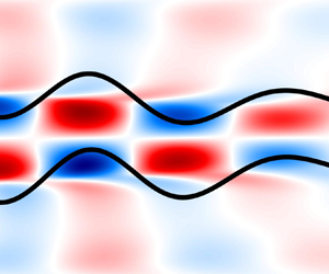
Following, Tammisola et al. (Reference Tammisola, Lundell and Söderberg2012), we compute the nonlinear flow for a variety of Weber numbers ranging from $We = 3.\bar {3}$ to $We = 16.\bar {6}$. In figure 2, the spectra obtained from the DMD and the corresponding mode shapes with the largest amplitude that dominate the flow are displayed for several investigated $We$ where an unsteady solution is found. The interface amplitude is overlayed on the modes. These are the same Weber numbers that are presented in Tammisola et al. (Reference Tammisola, Lundell and Söderberg2012).

Figure 2. (a) Magnitude of the DMD modes at each frequency, extracted from the nonlinear simulation. (b) Shapes of the dominant modes at the respective Weber numbers.

For Weber numbers larger than $We \approx 16$, all disturbances decay, and the flow settles to a steady solution. For $We = 12.5$, a periodic solution is seen that gives rise to a sinuous mode with its amplitude maximum located around $x = 8$. For increasing surface tension, at $We = 10$, three sinuous modes are observed. One mode is the same as seen for $We = 12.5$, which has moved slightly upstream (amplitude maximum $x = 7.5$) and has a lower frequency and amplitude. The second and third mode show a short-wave structure in the vicinity of the inlet, with the amplitude maximum located at around $x = 1.9$, and a long-wave structure located further downstream with an amplitude maximum around $x = 13$. These modes have a higher (almost similar) frequency and a generally larger amplitude than the first mode. Further, both of these modes display opposite slight asymmetries in the amplitude in the short-wave structure in the vicinity of the inlet. Note that, in figure 2(b), only one of these modes is shown. For $We = 6.\bar {6}$ three modes are found. The most energetic mode has a varicose structure with an amplitude maximum located at around $x = 4$. The other modes are the sinuous modes, observed for $We = 12.5$ and $We = 10$, with their amplitude maximum shifted far upstream. At $We = 5$ a single varicose mode with its amplitude maximum close to the inlet at around $x = 2.6$ is found. For even higher surface tension the flow becomes globally stable again, so that for $We = 3.\bar {3}$ a steady solution is obtained.

To give a broader overview over the complexity of the dynamics in the flow and see in which Weber number regime the dominant modes are unstable, their frequencies are plotted vs the respective Weber numbers in figure 3(a). Additionally, in figure 3(b) a bifurcation diagram is shown by plotting the local minima and maxima of the transversal velocity $v$ at $(x,y) = (5,0)$, within the time period after the saturation. From the above presentation it is seen that, under the influence of surface tension, the flow undergoes a series of bifurcations that gives rise to an increasingly complex modal interplay that governs the flow dynamics. Starting from a stable fixed point solution, a first Hopf bifurcation occurs between $We = 16.\bar {6}$ and $We = 12.5$ where the flow reaches a stable limit cycle, governed by a periodic oscillation produced by sinuous mode 1. In figure 3(b), this is characterised by a distinct minimum and maximum of $v$. A second mode, sinuous mode 2 bifurcates between $We = 12$ and $We = 11$. Both sinuous modes have incommensurate frequencies, resulting in a quasiperiodic motion and thus the limit cycle loses its stability to a torus. As noted above, a separate mode very similar to sinuous mode 2, with a slightly lower frequency is observed at $We = 10$. Both modes, sinuous mode 1 and 2, are still active at $We = 6.\bar {6}$ and vanish between $We = 6.\bar {6}$ and $We = 5$. Between $We = 9$ and $We = 8$ a third mode with an incommensurate frequency, varicose mode 1, emerges that governs the dynamics until the flow returns to a stable fixed point again between $We = 5$ and $We = 3.\bar {3}$. Additionally, as is seen in figure 2(a) for $We = 10$ and $We = 6.\bar {6}$, a dense set of frequency peaks around the dominating peaks, as well as some very low frequencies are seen in the spectra. While not shown, this behaviour is also visible in the spectra for other intermediate Weber numbers. Furthermore, for $We = 12.5, 5$ a more pronounced influence of the first harmonic mode is seen as compared to the other presented $We$. While a thorough investigation of these additional modes and their dynamics is beyond the scope of this work, they are likely the result of nonlinear interactions between the described modes and/or higher harmonics. As a result of the presence of several competing modes for $11 \leq We \leq 6.\bar {6}$, in this regime, the flow is attracted towards higher-dimensional states, characterised by quasiperiodic or chaotic oscillations. This is characterised in figure 3(b) by an increasingly dense variety of minima and maxima at the respective Weber numbers. In § 5.4 we will compare linear and nonlinear dynamics.

Figure 3. (a) Dominant frequencies of the appearing modes extracted from the DMD in the flow for all investigated Weber numbers. (b) Bifurcations illustrated by the min–max values of $v$ at $(x,y) = (5,0)$.

5.2. Base flows

For the validation of the linear solver, we choose the basic state solution obtained for $We_{base} = \infty$, as it bears closest resemblance to the results of Tammisola et al. (Reference Tammisola, Lundell and Söderberg2012) who obtained the base flow by computing a single-phase flow without interface and surface tension, exploiting the fact that in the absence of surface tension the flow is globally stable. The interface was introduced a posteriori by computing a streamline from $\boldsymbol {x}=(0,1)^{\textrm {T}}$. It was argued that, for this particular configuration, the curvature of the unperturbed interface is generally small, except for a small region very close to the inlet ($x<0.1$), and thus surface-tension-induced pressure gradients are probably negligible even for very high surface tension.

We have verified this assumption by computing the steady state solution at $We_{base} = \infty$, where the flow is globally stable, and $We_{base} = 12.5$, where the flow is only unstable for sinuous perturbations and thus can be obtained by imposing symmetry conditions at $y=0$. Additionally, we have computed the interface as a streamline on the single-phase base flow. The interface coordinates of the first two base flows are computed by reconstructing the piecewise linear interface segments from the respective volume fractions using the same routines that are used by the VOF advection scheme. The interface is plotted in figure 4(a) and the relative errors, with respect to the single phase flow, where a streamline is computed as interface, are given in table 1. For both, $We_{base} = \infty$ and $We_{base} = 12.5$, the error is below 1 %. The remaining error between the streamline interface and the interface for $We_{base} = \infty$ is probably rooted in the inaccuracy of the advection scheme as will be addressed in the next paragraph. The relative error of the base flow interface for increasing grid resolutions is shown in table 2. As is seen, the relative error between the highest and second highest resolution is again, below 1 %. For the present flow configuration it is therefore justified to use the base flow at $We_{base} = \infty$ for the linear computations.

Figure 4. (a) Interface position and (b) curvature of the respective base flows.

Table 1. Relative error of the basic state interface $I$. Errors are measured against the streamline-constructed interface of the single-phase flow $I_{s}$. The Weber numbers of the respective two-phase solutions are stated as subscripts.

Table 2. Convergence of the nonlinear and linear flow for increasing level of refinement. Shown is the relative error of the basic state interface for $We_{base} = \infty$, the convergence of the frequency $\mathrm {Im}(\lambda )$ of the dominant DMD mode of the nonlinear simulation and of the most unstable eigenvalue $\lambda$ of the linear analysis for $We = 12.5$.

It has to be noted that, despite the marginal differences between the interfaces of the basic states, the convergence of the case $We_{base} = 12.5$ is worse than for $We_{base} = \infty$ or for the case of the single-phase flow. While for the latter two cases an error $\|\boldsymbol {u}^{n+1}-\boldsymbol {u}^{n}\|_{\infty } =O(10^{-16})$ is reached, for the former it remains above $O(10^{-6})$. The reason for this behaviour is probably the occurrence of spurious currents. These are generally not considered an issue for equilibrium solutions of interfacial flows without velocity of the background fluid, when employing well-balanced schemes for computing the surface tension term. However, in the dynamic case where the background fluid has non-zero velocity, the problem persists due to numerical errors of the interface advection. These induce curvature errors which, again, induce errors in the velocity. As demonstrated in Popinet (Reference Popinet2009) for a translating droplet, the induced error in the velocity field is relatively insensitive to increased mesh resolution (its $L_\infty$ norm shows less than first-order convergence) and scales approximately with $We^{-1/2}$. The implications are readily seen in the curvature plot in figure 4(b). Since the $\kappa$ involves the second derivative of the height function of the interface, the numerical errors of the advection scheme produce significant oscillations in the curvature for $We_{base} = 12.5$. These are especially pronounced close to the inlet where the shear of the fluid streams is largest. To a lesser degree, these oscillations are also seen for $We_{base} = \infty$, but since the surface tension force is zero, there is no two-way coupling between the curvature and the velocity. Consequently, the disturbances are weaker and the convergence of the velocity field is not affected.

In preliminary computations we have assessed the effect of using finite Weber number base flows, as the one for $We_{base} = 12.5$, for the linear computations. However, due to the spurious advection errors in the base flow, spurious modes occurred in our results that hampered a successful analysis. Abadie, Aubin & Legendre (Reference Abadie, Aubin and Legendre2015) have shown that advection of the interface using a level set method may lead to a reduction of dynamic spurious currents as opposed to the VOF method that is used here. This could be a possible avenue towards reducing the base flow curvature errors for finite Weber numbers in a future study.

5.3. Computation of linear global modes

In § 5.1 we have seen that the action of surface tension on the base flow leads to a complex dynamics, with often several distinct modes being visible in the flow. Here, we investigate whether linear analysis can successfully predict the destabilisation that gives rise to the observed nonlinear dynamics. Further, we aim to compare the present linear results with those of Tammisola et al. (Reference Tammisola, Lundell and Söderberg2012). Therefore, we limit the analysis to the $We$ investigated in their study.

The computation of linear global modes is done by constructing a low-dimensional subspace representation of the linearised Navier–Stokes operator, using the Arnoldi method as outlined in § 4.2. The Krylov vectors spanning the subspace are obtained by time stepping of the linearised solver. The integration time $\tau$ between two consecutive snapshots is arbitrary, however, in order to satisfy the Nyquist criterion, at least two sample points are needed to resolve the highest desired frequency. Furthermore, too small values of $\tau$ may lead to insufficient temporal separation between consecutive Krylov vectors, thus hindering convergence of the method within a reasonable subspace dimension. In practice we choose $\tau = 1.5$. We have checked that the integration time, within the stated restrictions, does not influence the obtained results to a relevant degree. Arnoldi iterations are performed until a residual $\|\boldsymbol {A}\boldsymbol {\hat {q}}_j - \mu _j\boldsymbol {\hat {q}}_j\| < 10^{-6}$ for all unstable eigenvalues is reached. The grid independence is demonstrated in table 2 for the unstable eigenvalue, computed for $We = 12.5$.

The computed growth rates $\mathrm {Re}(\lambda )$ and frequencies $\mathrm {Im}(\lambda )$ are given in figure 5 for the stated Weber numbers. Both are compared to the results of Tammisola et al. (Reference Tammisola, Lundell and Söderberg2012). Further, the frequencies are compared to the mode frequencies obtained in the nonlinear simulation. The area within the dashed vertical lines corresponds to the range of Weber numbers where the nonlinear flow is unsteady. A direct comparison of the computed eigenvalues of the present study and those computed in Tammisola et al. (Reference Tammisola, Lundell and Söderberg2012) is given in table 3. Further, in figure 6(a) the growth rates, obtained from the linear analysis for $We = 5, 6.\bar {6}, 10, 12.5$, are compared to the disturbance growth in the nonlinear simulation. In figure 6(b), the shapes of the computed unstable modes are presented for each Weber number where the corresponding amplitude of the interface is plotted as black line and where the amplitude is chosen arbitrarily for suitable visualisation.

Figure 5. (a) Comparison of the mode frequencies and (b) growth rates at the respective Weber numbers.

Figure 6. (a) Comparison of the velocity disturbance growth of the nonlinear simulation $v$ at $(x,y) = (5,0)$ and the exponential growth rate of the most unstable linear global modes of the present analysis. (b) Mode shapes of the respective eigenmodes. The corresponding eigenvalue $\lambda$ is given for each mode.

Table 3. Eigenvalues $\lambda$ of the present linear analysis, the ones of Tammisola et al. (Reference Tammisola, Lundell and Söderberg2012) and frequencies $\mathrm {Im}(\lambda )$ of the dominant DMD modes of the nonlinear simulation at the respective Weber numbers.

The frequency values of the linear analysis and their nonlinear equivalents are very similar in all cases. They compare especially well in the upper regime of unstable Weber numbers, for $We = 10$ and $We = 12.5$. In both cases, all unstable modes are sinuous. In line with the nonlinear simulation, sinuous mode 1 from $We = 12.5$ is still unstable for $We = 10$ and $We = 6.\bar {6}$ and the appearance of sinuous mode 2, that is the most unstable mode for $We = 10$ and remains unstable for $We = 6.\bar {6}$, is accurately predicted. The predicted mode shapes at both $We$ show good agreement compared to the DMD modes in figure 2(b), both in terms of shape and streamwise position of the amplitude maximum. For $We = 6.\bar {6}$, the most unstable mode is varicose mode 1. In contrast to the computed DMD modes, the linear global modes at $We = 6.\bar {6}$ show a more regular and symmetric structure and their frequencies are slightly over-predicted. We believe this is not a shortcoming of the linear analysis but rather an indication that the quasiperiodicity of the dynamics induces non-negligible nonlinear interactions in the flow that lead to a departure of from the linear dynamics presented here. For $We = 5$, varicose mode 1 is the only unstable mode predicted. Its frequency is, again, slightly over-predicted which again can be attributed to a non-negligible nonlinearity in the flow dynamics.

Turning to the growth rates, in figure 6(a) a comparison of the present growth rates with the energy growth of the nonlinear simulation is shown. Therefore, we initialise the nonlinear flow from the steady base flow with $We_{base} = \infty$ and monitor the disturbance growth via the $v$ component of the velocity at $(x,y) = (5,0)$ where $V = 0$. The plotted time series of the nonlinear energy growth is obtained by computing the logarithm of the envelope of the modulus of the monitored velocity signal. The lines representing the growth rates of the linear analysis are shifted for suitable alignment with the nonlinear time series. For $We = 12.5$, a sufficiently long time interval of approximately exponential growth is seen that is in agreement with the obtained growth rates. For $We = 10$ and $We = 6.\bar {6}$, intervals of exponential growth are less clear which may be due to the competing modes that are observed at this Weber numbers and that prevent a clear exponential growth of a single mode from being observed. Furthermore it could be hypothesised that transient growth leads to short time amplification of additional modes that further influence the observed energy growth. Nevertheless, the modal growth rates obtained in the linear analysis agree reasonably well with the overall energy growth, observed in the nonlinear flow at $We = 10, 6.\bar {6}$. For $We = 5$, an interval of clear exponential growth is seen that is in good agreement with the predicted growth rate of the linear analysis.

Comparing the present results to the study of Tammisola et al. (Reference Tammisola, Lundell and Söderberg2012), good agreement is seen between the computed mode frequencies and those of Tammisola et al. (Reference Tammisola, Lundell and Söderberg2012). In particular, both linear analyses show similar over-predictions of the frequencies for $We = 5, 6.\bar {6}$. On the other hand, the present growth rates show notable deviations, compared to their results. For $We = 6.\bar {6}, 10, 12.5, 16.\bar {6}$ the present growth rates are always higher, up to almost a factor of 2, whereas for $We = 3.\bar {3}$ they are notably lower. The prediction of the bifurcation points also differs. For $We = 3.\bar {3}$, Tammisola et al. (Reference Tammisola, Lundell and Söderberg2012) still predict an unstable eigenvalue, while in the present study, the flow is already linearly stable, consistent with the nonlinear simulation. Several reasons for the different growth rates in both studies may be found. Generally, the growth rates obtained in both analyses are rather small for all computed Weber numbers. Therefore, slight differences in the employed numerical schemes may lead to large relative changes in the growth rates. From a numerical perspective, the treatment of the interface and surface tension via separate domains and coupling conditions in Tammisola et al. (Reference Tammisola, Lundell and Söderberg2012) might be a source for differences. Further, the use of Chebyshev polynomials in their study, while spectrally accurate, introduces a non-uniform grid spacing which leads to a reduced resolution in the centre of the respective domains. Another possible reason is the use of a streamline-based reconstruction of the interface which is shown to result in a slightly smaller interface curvature, as seen in figure 4(b). These differences are especially prominent close to the inlet, where the global mode at this Weber number is localised.

5.4. Comparison of nonlinear and linear dynamics

In §§ 5.1 and 5.3 we have analysed the nonlinear and linear dynamics of plane wakes under the influence of surface tension and have found that the linear analysis reliably predicts the dominant modes, seen in the nonlinear flow, to be linearly unstable. However, from figure 2(a) it is as well seen that for the intermediate Weber numbers studied there, the nonlinear dynamics contains significantly more modes than the linear analysis predicts. Hence, these modes are the result of nonlinear harmonic interactions resulting from the quadratic nonlinearity of the advection term or the higher-order geometric nonlinearity of the surface tension term. It is therefore worthwhile to shed more light on the validity of the linear dynamics for approximating the nonlinear flow. To this end, we use the dominant DMD modes that are shown in figure 2(b), and which we have seen to closely correspond to the linear modes presented figure 6(b) and table 3, to construct a low-dimensional approximation of the nonlinear dynamics of the flow.

The departure of the linear dynamics towards the full nonlinear dynamics can be analysed by employing the time-averaged mean flow, as has been shown in various works in recent times (e.g. Barkley Reference Barkley2006; Oberleithner, Rukes & Soria Reference Oberleithner, Rukes and Soria2014; Boujo, Bauerheim & Noiray Reference Boujo, Bauerheim and Noiray2018; Schmidt & Oberleithner Reference Schmidt and Oberleithner2020). According to the theory established therein, the nonlinear saturation process is driven by the interaction of higher harmonics with their complex conjugates through the Reynolds stress divergence that modifies the base flow towards the mean flow. As a consequence, eigenmodes that are unstable with respect to the base flow become marginally stable on the mean flow. Simultaneously, the mean flow modification may alter the structure and frequency of the eigenmodes through the linear perturbation equation. The remaining difference from the full nonlinear flow is accounted for by nonlinear interactions between different harmonics. In the present work, the frequencies of the linear modes are in close correspondence to their equivalent nonlinear modes which indicates that these modes are not significantly affected by the mean flow modification. Hence, the constructed model can be seen as a representation of the linear dynamics around the mean flow. The difference between the reduced and full dynamics is the nonlinear interactions between different harmonics and, thus, it is reasonable to assume that a comparison of the reconstructed and full dynamics yields an appropriate qualitative picture of how far the linear and nonlinear dynamics are apart.

In figure 7, we present velocity phase trajectories of the full and reconstructed dynamics using probes located at the approximate streamwise location of the respective amplitude maxima of the oscillation of the nonlinear flow. For a clean visual representation, we plot the velocity histories using a time lag of one period $\tau = 1/\mathrm {Im}(\lambda )$ where $\mathrm {Im}(\lambda )$ is chosen as the frequency of the mode with the largest amplitude for each respective Weber number (i.e. sinuous mode 1 ($We = 12.5$), sinuous mode 2 ($We = 10$), varicose mode 1 ($We = 6.\bar {6},5$)). To get a better view of the cross-sections of the phase space we plot a variant of Poincaré sections in figure 8. The section is chosen such that the phase trajectory crosses it every completed cycle $n$, established by the period $\tau$.

Figure 7. Qualitative representation of the velocity phase trajectories at $(x,y) = (8,0)$ ($We = 12.5$), $(x,y) = (8,0)$ ($We = 10$), $(x,y) = (6,0)$ ($We = 6.\bar {6}$) and $(x,y) = (4,0)$ ($We = 5$). The upper row in black shows the full dynamics and the lower row in blue the reconstructed dynamics. All plots are equally scaled.

Figure 8. Qualitative Poincaré sections of the trajectories presented in figure 7. Sections are chosen such that trajectories cross every completed cycle $n$. The upper row in black shows the full dynamics and the lower row in blue the reconstructed dynamics. All plots are equally scaled.

As is expected from the analysis in § 5.1, for $We = 12.5$ and $We = 5$, the full nonlinear dynamics is represented by a limit cycle. Thus a closed orbit is seen in figure 7 which, however, shows a notable deformation, caused by higher harmonic modes. The reconstructed mono-frequent dynamics lacks this higher harmonic influence which results in a slightly smaller orbit and thus a reduced velocity amplitude. As expected for a limit-cycle solution, both trajectories cross the section plane at a fixed point in figure 8. For $We = 10$ and $We = 6.\bar {6}$, the trajectories of the full nonlinear dynamics show complex patterns and the orbits fill a closed region in the phase space, possibly indicating chaotic behaviour. The reconstructed dynamics each consists of three incommensurate frequencies, thus forming a quasiperiodic cycle on a 3-torus. The reconstruction shows a significantly different behaviour compared to the full dynamics and particularly for $We = 10$ results in a overall lower amplitude oscillation. For both Weber numbers, the section plots in figure 8 show the trajectory crossings clustered broadly around the fixed points, observed for $We = 12.5, 5$. While the crossings of the reconstructed dynamics show regular closed paths, indicative of quasiperiodicity, the full dynamics does not exhibit clear paths, again suggesting a chaotic behaviour.