


1. Introduction
Macroalgae, also known as seaweeds, are an important component in temperate marine ecosystems (Dayton Reference Dayton1985; Schiel & Forster Reference Schiel and Forster2015). Providing shelter, food and protection for many species of marine living creatures, macroalgae play a paramount role in preserving biodiversity and promoting sustainable aquaculture production. Macroalgal forest harvesting also contributes enormously to various applications, such as remediation of eutrophication pollution, biofuel production, food and pharmaceutical processing, etc. The desire to increase the productivity of aquaculture spurs the growing need for aquafarm development in the ocean, where the canopy grows near the surface and is supported by a floating structure (Troell et al. Reference Troell, Joyce, Chopin, Neori, Buschmann and Fang2009; Stevens & Petersen Reference Stevens and Petersen2011). The macroalgal canopy alters the surrounding flow conditions by dampening the currents and wave motions (Rosman et al. Reference Rosman, Koseff, Monismith and Grover2007). These flow modifications have profound implications for the nutrient uptake and associated processes of sedimentation and recruitment (Duggins, Eckman & Sewell Reference Duggins, Eckman and Sewell1990; Plew Reference Plew2011b). Therefore, understanding and quantifying the diverse hydrodynamic processes that occur in the presence of macroalgal farms is essential in evaluating and designing optimal farm configurations, as well as assessing their environmental impacts.
From a hydrodynamics perspective, aquatic vegetation can be classified as submerged, emergent or suspended based on its growth form. Submerged and emergent vegetation are attached to the bottom floor, and occupy a fraction or all of the water depth. The flow structures and mass transport over such canopies have been well documented (Nepf Reference Nepf2012a,Reference Nepfb; Yan et al. Reference Yan, Nepf, Huang and Cui2017). Particular attention has been given to the shear layer turbulence at the canopy top (for submerged canopy), which prompts the generation of canopy-scale coherent structures that dominate the momentum and scalar exchanges between the canopy and the free flow above. Suspended canopies, such as the macroalgal farm considered here, extend downward from the surface and occupy the upper part of the water body (Plew et al. Reference Plew, Stevens, Spigel and Hartstein2005, Reference Plew, Spigel, Stevens, Nokes and Davidson2006; Stevens & Petersen Reference Stevens and Petersen2011). The flow and canopy interactions for this configuration remain less explored as compared to the bottom-mounted counterpart (Stevens & Plew Reference Stevens and Plew2019).
For suspended vegetation, the vertical discontinuity in drag beneath the canopy also leads to a shear layer, which penetrates a finite distance into the canopy and mediates the turbulent exchanges between the canopy and the underlying flow (Plew Reference Plew2011a). Through laboratory experiments of suspended canopies in shallow waters, Plew (Reference Plew2011a) concluded that the additional bottom boundary layer (BBL) associated with the ocean floor affects the penetration of the shear layer into the suspended canopy. Based on the measurements of Plew (Reference Plew2011a), Huai et al. (Reference Huai, Hu, Zeng and Han2012) proposed a simple analytical model for the vertical profile of streamwise velocity. While these studies focus on flow over uniform canopies (i.e. essentially infinite size), where the flow has been fully adjusted to the canopy, common aquaculture structures are of finite size and the corresponding canopy flow displays distinct spatial distribution patterns.
The finite dimensions and spatial arrangement of the suspended canopy lead to flow patterns different from the fully developed scenario (Tseung, Kikkert & Plew Reference Tseung, Kikkert and Plew2016). According to Tseung et al. (Reference Tseung, Kikkert and Plew2016) and Zhao, Huai & Li (Reference Zhao, Huai and Li2017), the flow over a suspended canopy of finite size is similar to the terrestrial flow over forest patches (Belcher, Jerram & Hunt Reference Belcher, Jerram and Hunt2003), and it can be divided into four zones of distinct mean flow behaviour in the downstream direction: (i) the upstream adjustment zone, (ii) the transition zone, (iii) the fully developed zone and (iv) the wake zone. The distance over which the velocity profile reaches a fully developed state is affected by canopy geometry (e.g. plant density and stem diameter) (Rosman et al. Reference Rosman, Monismith, Denny and Koseff2010). Zhou & Venayagamoorthy (Reference Zhou and Venayagamoorthy2019) examined the effect of a circular patch of suspended canopy on the mean flow dynamics in deep water, and found out that the patch geometry poses another impact on the adjustment of flow pathways. In the light of these studies, we are motivated by the water flow over an aquaculture farm of finite size in the deep ocean, and seek to explore how the ocean mixed layer (OML) evolves as it approaches and flows over the farm under typical ocean conditions.
In the marine environment, ocean waves have a profound influence on the water flow and the exchange of nutrients between kelp forests and ambient water. In many studies, this effect is characterized in terms of the Stokes drift (Gaylord et al. Reference Gaylord2007; Rosman et al. Reference Rosman, Koseff, Monismith and Grover2007), which refers to the net motion of fluid parcels in the direction of wave propagation that arises from the unclosed orbital motions for finite amplitude waves (Monismith & Fong Reference Monismith and Fong2004). Rosman et al. (Reference Rosman, Koseff, Monismith and Grover2007) explored the effects of giant kelp forests on ocean flows through a field experiment at the coast of Santa Cruz, California. They highlighted the importance of the Stokes drift in cross-shore transport within the kelp canopy. Rosman et al. (Reference Rosman, Denny, Zeller, Monismith and Koseff2013) conducted experiments at a scaled laboratory flume to examine the interaction of surface waves and currents with kelp forests, and concluded that these interactions must be taken into account when modelling flow and transport within kelp forests.
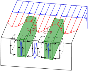
One of the distinct features widely observed in the upper ocean is the presence of Langmuir circulations, which consists of counter-rotating vortices near the ocean surface roughly aligned with the wind direction (Thorpe Reference Thorpe2004). It is well accepted that the Langmuir circulations are generated by the interaction between the wind-driven shear current and the Stokes drift velocity induced by the surface gravity waves through the the Craik–Leibovich (CL) type 2 instability (Craik Reference Craik1977; Leibovich Reference Leibovich1983). The associated ocean flows are referred to as Langmuir turbulence (McWiliams, Sullivan & Moeng Reference McWiliams, Sullivan and Moeng1997), which can be numerically modelled by adding a vortex force into the momentum equation without the need to resolve the surface gravity waves (Skyllingstad & Denbo Reference Skyllingstad and Denbo1995; McWiliams et al. Reference McWiliams, Sullivan and Moeng1997; Yang et al. Reference Yang, Chen, Chamecki and Meneveau2015; Chamecki et al. Reference Chamecki, Chor, Yang and Meneveau2019). The increased level of turbulence intensity promoted by Langmuir circulations is expected to affect the supply and uptake of nutrients within the marine ecosystem (Barton et al. Reference Barton, Ward, Williams and Follows2014).
In this study, we use a fine-scale large eddy simulation (LES) model to explore the development of an OML in the presence of a large macroalgal farm under typical current and wave regimes. The main goal of the present work is to characterize the hydrodynamics around a macroalgal suspended farm and advance our understanding of canopy flows in the ocean. We assume that the ocean is deep enough so that the flow is free from the complexities of BBL. Section 2 describes the numerical approach for modelling oceanic boundary layer flow over a macroalgal canopy. A triple-decomposition strategy is used to separate the flow field into the contributions due to mean flow, secondary flow resulting from the farm drag and transient fluctuations. Section 3 describes the main characteristics of the flow field and the emergence of persistent flow structures termed ‘attached Langmuir circulations’. Section 4 discusses the underlying mechanism of generation of attached Langmuir circulations, and characterizes their spatial development. Section 5 describes the energy conversion among the three components of the flow field. Conclusions are drawn in § 6.
2. Methods
2.1. Mathematical model
For the past three decades, the LES technique has been widely adopted to study turbulence in the OML. Detailed discussion of the LES framework and assumptions underpinning its applicability can be found in the review paper by Chamecki et al. (Reference Chamecki, Chor, Yang and Meneveau2019). In the present work, the dynamics of Langmuir turbulence in the presence of a macroalgal canopy is captured using the LES method by solving the wave-averaged equations described by McWiliams et al. (Reference McWiliams, Sullivan and Moeng1997). This mathematical model is built upon the original CL equations (Craik & Leibovich Reference Craik and Leibovich1976) with the inclusion of planetary rotation and Stokes drift advection of scalar fields,
 \begin{gather} \boldsymbol{\nabla}\boldsymbol{\cdot}{\widetilde{\boldsymbol{u}}}=0, \end{gather}
 \begin{gather} \frac{\partial{\widetilde{\boldsymbol{u}}}}{\partial{t}}+{\widetilde{\boldsymbol{u}}} \boldsymbol{\cdot}\boldsymbol{\nabla}{\widetilde{\boldsymbol{u}}} ={-} \boldsymbol{\nabla}{\varPi}-f\boldsymbol{e_z}\times \left(\widetilde{\boldsymbol{u}}+\boldsymbol{u}_s-\boldsymbol{u}_g\right) \nonumber\\ \qquad\qquad\qquad\qquad\qquad\qquad\qquad +\,\boldsymbol{u}_s \times \widetilde{\boldsymbol{\zeta}}+ \left(1-\frac{\widetilde{\rho}}{\rho_0}\right)g\boldsymbol{e_z}+\boldsymbol{\nabla} \boldsymbol{\cdot}{{\boldsymbol{\tau}}^d}-\boldsymbol{F}_D, \end{gather}
 \begin{gather} \frac{\partial{\widetilde{\rho}}}{\partial{t}}+ \left(\widetilde{\boldsymbol{u}}+ \boldsymbol{u}_s\right) \boldsymbol{\cdot}\boldsymbol{\nabla} \widetilde{\rho}=\boldsymbol{\nabla}\boldsymbol{\cdot}{\boldsymbol{\tau}_\rho}, \end{gather}
Here, the tilde indicates grid-filtered variables,  $\widetilde {\rho }$ is the filtered seawater density,
  $\rho _0$ is the reference density,
  $\varPi$ is the generalized pressure,
  $f$ is the Coriolis frequency,
  $g=9.81\ \mathrm {m}\ \textrm {s}^{-2}$ is the gravitational acceleration,
  $\boldsymbol {e_z}$ is the unit vector in the vertical direction and
  ${\widetilde {\boldsymbol {u}}}=({\widetilde {u}, \widetilde {v}, \widetilde {w}})$ is the velocity vector represented in the Cartesian coordinate system
  $\boldsymbol {x}=({x}, {y}, {z})$, with
  $x$,
$x$,  $y$ and
  $z$ being the downstream, cross-stream and vertical directions, respectively. The vertical coordinate is defined positive upward with
  $z=0$ at the ocean surface. The geostrophic current
  $\boldsymbol {u}_{g}=(u_g, 0, 0)$ is driven by an external mean pressure gradient force with magnitude
  $fu_g$ applied in the
  $y$-direction. The canopy is treated as a source of flow resistance, and its effect is accounted for by adding a drag force
  $\boldsymbol {F}_D$ to the momentum equation.
In (2.2) and (2.3),  ${\boldsymbol {\tau }^d}$ is the deviatoric part of the subgrid-scale (SGS) stress tensor
  $\boldsymbol {\tau } =\widetilde {\boldsymbol {u}}\widetilde {\boldsymbol {u}}-\widetilde {\boldsymbol {u}\boldsymbol {u}}$, and
  ${\boldsymbol {\tau }_\rho } = \widetilde {\boldsymbol {u}}\widetilde {\rho }-\widetilde {\boldsymbol {u}\rho }$ is the SGS buoyancy flux. We assume that the changes in the seawater density
  $\rho$ are caused by the varying potential temperature
  $\theta$, and these two variables are linearly related by
  $\rho =\rho _0[1-\alpha (\theta -\theta _0)]$, where
  $\alpha =2\times 10^{-4}\ \mathrm {K}^{-1}$ is the thermal expansion coefficient, and
  $\theta _0$ is the reference potential temperature at which
  $\rho _0$ is measured. The SGS stress tensor is modelled using the Lagrangian scale-dependent dynamic Smagorinsky SGS model (Bou-Zeid, Meneveau & Parlange Reference Bou-Zeid, Meneveau and Parlange2005). Then, the SGS buoyancy flux is parameterized using an eddy diffusivity closure with a prescribed value of SGS Prandtl number
  $Pr_t=0.4$. The viscous force is assumed to be negligible for the high Reynolds number flows considered in the present study.
The Stokes drift  $\boldsymbol {u}_{s}$ induced by surface gravity waves is imposed in the governing equations to reflect the time-averaged effects of the wave field on the oceanic turbulence, since the surface wave motions are not explicitly resolved in our simulations. The third term on the right-hand side of (2.2) is the CL vortex force
  $\boldsymbol {u}_s \times \widetilde {\boldsymbol {\zeta }}$ (here
  $\widetilde {\boldsymbol {\zeta }}=\boldsymbol {\nabla }\times \widetilde {\boldsymbol {u}}$ is the vorticity field), which represents the interaction of wind-driven turbulence and surface gravity waves. For simplicity, we only consider a steady monochromatic wave. Assuming that the surface gravity wave propagates along the mean wind direction (i.e. the
  $x$-direction), the Stoke drift velocity reduces to
  $\boldsymbol {u}_{s}=(u_s(z), 0, 0)$, where
  $u_s$ is given by
 \begin{equation} u_s={U_s}\,\textrm{e}^{2kz}, \end{equation}
in which  $k$ is the wavenumber and
  $U_s$ is the wave-induced Stokes drift at the surface. Then, the vortex force
  $\boldsymbol {u}_s \times \widetilde {\boldsymbol {\zeta }}$ reduces to
  $(0, -u_s \widetilde {\zeta }_z, u_s \widetilde {\zeta }_y)$. Note that the presence of the canopy can attenuate the waves and impact the Stokes drift profile (Rosman et al. Reference Rosman, Denny, Zeller, Monismith and Koseff2013). Based on the approach developed by Dalrymple, Kirby & Hwang (Reference Dalrymple, Kirby and Hwang1984), we have estimated the effects of canopy drag on the surface waves for the specific canopy and wave parameters used in this study and found only a small attenuation of approximately
  $3\,\%$ in wave amplitude and
  $6\,\%$ in the magnitude of the Stokes drift (see Appendix B). These estimates are consistent with those obtained in flume measurements by Rosman et al. (Reference Rosman, Denny, Zeller, Monismith and Koseff2013). For the sake of simplicity, we neglect wave attenuation in this study.
Finally, there is evidence suggesting that surface waves can induce a mean current in the direction of the wave propagation within aquatic canopies (Luhar et al. Reference Luhar, Coutu, Infantes, Fox and Nepf2010, Reference Luhar, Infantes, Orfila, Terrados and Nepf2013; Abdolahpour, Hambleton & Ghisalberti Reference Abdolahpour, Hambleton and Ghisalberti2017; Chen, Liu & Zou Reference Chen, Liu and Zou2019; van Rooijen et al. Reference van Rooijen, Lowe, Rijnsdorp, Ghisalberti, Jacobsen and McCall2020). This wave-induced current is caused mainly by the reduction of the wave orbital velocity within the canopy, and inclusion in our model would require explicitly resolving the surface waves. We used the empirical results in the literature (see Abdolahpour et al. Reference Abdolahpour, Hambleton and Ghisalberti2017; Chen et al. Reference Chen, Liu and Zou2019) to estimate the maximum magnitude of this wave-induced current for the suspended farm simulated here, and found out that it is a reasonably small fraction (approximately 20 %) of the steady geostrophic current  $u_g$ imposed in our simulations. Thus, we expect the overall effects of this wave-induced current to be small, and we neglect them in adopting a wave-averaged approach.
2.2. Numerical representation of macroalgal farm
For the cultivation of macroalgae, the aquaculture structures being deployed in the open ocean are varied, but common practice is to suspend seeded materials from surface buoys and mooring structures (Charrier, Wichard & Reddy Reference Charrier, Wichard and Reddy2018). One possible configuration for the cultivation strategy for the macroalgae of interest (giant kelp) is shown in figure 1(a). The macroalgal farm comprises parallel lines of seeded growing ropes with a length of  $W_{MF}=8$ m coiled around a backbone (or longline). Each backbone line, with a length
  $L_{MF}$, is anchored at each end and connected to surface buoys (not shown). Each macroalgae consists of 8 fronds with an average length
  $h_{MF}=19$ m, which are assumed to be in an upright posture by virtue of the buoyancy provided by the gas-filled floats (called pneumatocysts). The lateral spacing between two adjacent rows of canopy elements is
  $S_{MF}=26$ m.

Figure 1. Schematic of the spatial morphology of the suspended macroalgal farm: (a) spatial arrangement of the macroalgal farm; (b) frond area density profile for each row of macroalgal canopy,  $a(z)$, normalized by the canopy height
  $h_{MF}$.
The frond surface area of the cultivated macroalgae species is obtained by conversion of vertically resolved algal biomass generated from a macroalgal growth model (C. Frieder, personal communication) using allometric relationships (Fram et al. Reference Fram, Stewart, Brzezinski, Gaylord, Reed, Williams and MacIntyre2008). To simplify the numerical modelling, the frond surface area is redistributed uniformly within each canopy row in the horizontal directions, while the spatial arrangement of the row structure is resolved in the simulation. The fraction occupied by macroalgae has a total foliage area density (FAD) profile denoted as  $a(z)$, which is shown in figure 1(b). FAD is the total (one-sided) frond surface area per unit volume of space (
 $\mathrm {m}^{-1}$), without explicit differentiation among blades, fronds and stipes, etc. Since our main focus here is to examine the adjustment of OML as it flows over the farm, canopy parameters such as
  $a(z)$,
  $h_{MF}$,
  $S_{MF}$ are kept constant (the only exception being the length
  $L_{MF}$) and a sensitivity study to farm design is beyond the scope of this study.
The drag per unit mass  $\boldsymbol {F}_D$ in (2.2) represents the effect of the canopy as a momentum sink for the flow field, and it is parameterized as (Shaw & Schumann Reference Shaw and Schumann1992; Pan, Chamecki & Isard Reference Pan, Chamecki and Isard2014),
 \begin{equation} \boldsymbol{F}_D=\tfrac{1}{2}C_D a(z){\boldsymbol{\mathsf{P}}} \boldsymbol{\cdot}|\widetilde{\boldsymbol{u}}| \widetilde{\boldsymbol{u}}, \end{equation}
in which  $C_D$ is the drag coefficient and
  $|\widetilde {\boldsymbol {u}}|$ is the magnitude of the resolved velocity vector. For the sake of simplicity, the tilde symbols used to denote resolved variables are omitted hereafter. The coefficient tensor
  ${\boldsymbol{\mathsf{P}}} = P_x\boldsymbol {e_x}\boldsymbol {e_x} + P_x\boldsymbol {e_y}\boldsymbol {e_y} + P_z\boldsymbol {e_z}\boldsymbol {e_z}$ is employed here to account for the projection of total foliage area onto the orthogonal planes with normal in each one of the Cartesian directions. Note that the expression for
  ${\boldsymbol{\mathsf{P}}}$ involves the dyadic products of the standard basis vectors
  $\boldsymbol {e_x}$,
  $\boldsymbol {e_y}$ and
  $\boldsymbol {e_z}$, so that
  ${\boldsymbol{\mathsf{P}}}$ is also a second-order tensor. This projection operation is commonly used for terrestrial canopies (Legg & Powell Reference Legg and Powell1979; Aylor & Flesch Reference Aylor and Flesch2001; Pan et al. Reference Pan, Chamecki and Isard2014), and the coefficients
  $P_x$,
  $P_y$ and
  $P_z$ depend on the geometry of the canopy and thus on the specific details of each plant species (Aylor & Flesch Reference Aylor and Flesch2001). In the absence of observational data to specify these coefficients, we make the assumption of isotropic distribution of FAD (e.g. the fraction of FAD projected towards each direction is always the same), which corresponds to
  $P_x = P_y = P_z = 1/2$.
The drag coefficient  $C_D$ is a key input parameter in the drag model (2.5) that can affect the accuracy for the prediction of turbulence statistics (Pinard & Wilson Reference Pinard and Wilson2001). Generally,
  $C_D$ is estimated from the reduced momentum balance based on experimental measurements, where large uncertainty exists depending on the formulations of the momentum equation being used (Cescatti & Marcolla Reference Cescatti and Marcolla2004; Pan, Chamecki & Nepf Reference Pan, Chamecki and Nepf2016) and quality of measurements (Pinard & Wilson Reference Pinard and Wilson2001; Marcolla, Pitacco & Cescatti Reference Marcolla, Pitacco and Cescatti2003). Many numerical studies of atmospheric boundary layer flows used a height-averaged
  $C_D$ of constant value for terrestrial canopies (Shaw & Schumann Reference Shaw and Schumann1992; Dupont & Brunet Reference Dupont and Brunet2008; Finnigan, Shaw & Patton Reference Finnigan, Shaw and Patton2009). For a flexible canopy like that of macroalgae, the canopy elements can bend back and forth with the moving water, leading to reduced fluid drag relative to the rigid and upright vegetation (Boller & Carrington Reference Boller and Carrington2006; Luhar & Nepf Reference Luhar and Nepf2011). Pan et al. (Reference Pan, Chamecki and Isard2014) introduced a velocity-dependent
  $C_D$ in their LES study to account for the reconfiguration of a flexible cornfield in response to the surrounding flow (Vogel Reference Vogel1989). However, giant kelp elements do not bend with the flowing water in the same way as many terrestrial plants or seagrasses do, because they possess many gas-filled floats that can keep the fronds upward to the surface via buoyancy forces (Koehl & Wainwright Reference Koehl and Wainwright1977; Henderson Reference Henderson2019). In our LES cases, we use the value of
  $C_D = 0.0148$ reported in the experimental study of Utter & Denny (Reference Utter and Denny1996), which measured the drag coefficient on Macrocystis pyrifera fronds by towing a single plant from a boat in a field experiment. It should be noted that Utter & Denny (Reference Utter and Denny1996) modelled the canopy drag by a power law of the local velocity with an exponent of 1.6 to account for the drag reduction resulting from plant reconfiguration, while we assume the relationship between these two variables to be quadratic (2.5).
Apart from the fluid drag force, macroalgae are subjected to elastic and buoyant forces, both of which act to resist bending. The subtle balance among these forces determines the posture of macroalgae (Luhar & Nepf Reference Luhar and Nepf2011; Henderson Reference Henderson2019). Estimates given in Appendix A show that kelp stipes remain approximately upright in the flow, except for an oscillatory motion with amplitude comparable to the wave orbital displacement. In fact, this assumption is implicit in the parametric model for the drag force (2.5): the wave orbital velocity is not included in the drag calculation, implying that macroalgae oscillate with the wave orbital velocity (note that this assumption is consistent with the idea that the macroalgal canopy does not impact the waves).
2.3. Numerical scheme
The present LES framework employs a Cartesian grid using a vertically staggered arrangement, with the horizontal velocity components, pressure and potential temperature  $(u, v, p, \theta )$ defined at the cell centre, while the vertical velocity component
  $(w)$ is stored at the cell face. Spatial derivatives in the horizontal directions are treated with pseudo-spectral differentiation, while the derivatives in the vertical direction are discretized using a second-order centred-difference scheme. Aliasing errors associated with the nonlinear terms are removed via padding based on the 3/2 rule. Time advancement is performed using the fully explicit second-order accurate Adams–Bashforth scheme. The numerical code has been validated against the LES study of McWiliams et al. (Reference McWiliams, Sullivan and Moeng1997) for Langmuir turbulence in the deep ocean by Yang et al. (Reference Yang, Chen, Chamecki and Meneveau2015).
The LES domain with dimensions of  $L_x \times L_y \times L_z$ is shown in figure 2. For clarity, the origin of the coordinate system is defined at the leading edge of the farm in the central longitudinal plane, and the
  $z$-axis is pointing upward. The top boundary is specified as a non-deforming surface exposed to wind shear stress. A sponge layer is imposed within the bottom 20 % of the domain to damp out fluctuations of velocity and temperature, thus avoiding the reflection of the internal gravity waves.

Figure 2. Sketch of the LES computational model for Langmuir turbulence with the presence of suspended macroalgal farm in the deep ocean: (a) side view and (b) plan view. A fringe region of length  $L_{fr}$ towards the end of the domain is used to force the velocity and potential temperature back to the inflow, so periodic conditions are satisfied in the horizontal plane.
The backbone line is at a depth  $h_{b}=20$ m below the surface while the canopy height is
  $h_{MF}=19$ m, leaving a canopy-free layer at the top 1 m near the ocean surface to represent typical harvest practices. A domain depth of
  $L_z=6h_{b}$ is chosen to avoid interference with the bottom boundary condition as the flow is deflected below the canopy. The cross-stream domain size
  $L_y=8S_{MF}$ is tailored to encompass
  $N=8$ parallel rows of macroalgae, the longitudinal axes of which are aligned in the downstream direction. Periodic boundary conditions are imposed in the horizontal directions, which will enable us to exclude the complexities brought by the limited width of the farm. The inlet is positioned
  $L_u=7.5h_{b}$ upstream of the farm leading edge, and the outlet is at a distance
  $L_d=12.5h_{b}$ downstream of the farm trailing edge. Thus, the domain size in the downstream direction is
  $L_x = L_{MF}+20h_{b}$.
A fringe region of length  $L_{fr}=5h_{b}$ is used at the end of the domain (see figure 2) to enable simulations of spatially evolving boundary layer flows in a periodic domain using pseudo-spectral numerics (Stevens, Graham & Meneveau Reference Stevens, Graham and Meneveau2014). Specifically, the inflow turbulence profile at the inlet of the domain is provided by a precursor simulation carried out with identical conditions in the absence of the farm. After the precursor simulation reaches a fully developed turbulence regime, a region of length
  $L_{fr}$ is duplicated from the precursor simulation on the fringe region of the actual simulation at the end of every time step. Then, any variable
  $\phi$ (i.e. velocity and potential temperature) in the fringe region is determined as a weighted average of fields in the precursor and actual simulations (also see Stevens et al. Reference Stevens, Graham and Meneveau2014),
 \begin{equation} \phi(x,y,z,t) = f(x) \cdot \phi_{pre}(x,y,z,t) + \left[1-f(x)\right] \cdot \phi_{act}(x,y,z,t), \end{equation}
in which  $\phi _{pre}$ and
  $\phi _{act}$ are, respectively, the field in the precursor and actual domains, and
  $f(x)$ is the weighting function expressed as,
 \begin{equation} f(x) = \left\{\begin{array}{@{}ll} \dfrac{1}{2}\left[ 1 - \cos{\left({\rm \pi} \dfrac{x-x_s}{x_e-x_s} \right)} \right], & x_s \le x \le x_e \\ 1, & x > x_e. \end{array}\right. \end{equation}
Here,  $x$ represents the downstream position,
  $x_s=L_x-L_u-L_{fr}$ is the starting point of the fringe region and
  $x_e = L_x-L_u-\frac {1}{4}L_{fr}$ is the position beyond which
  $\phi =\phi _{pre}$. The length of the fringe region must be large enough to enable a smooth transition of the field
  $\phi$ from the farm wake flow to the inflow condition. To avoid any possible upstream influence from the fringe region, only solutions up to
  $x=x_s-3h_{b}$ are analysed.
2.4. Simulation parameters
Our major goal is to report new flow features that develop around suspended aquafarms under realistic oceanic conditions. Therefore, instead of exploring the vast parameter space of possible ocean states (e.g. varying degrees of wind, waves, currents and surface buoyancy forcing, etc.), we only focus on one set of very typical conditions encountered in the deep ocean. The flow is driven by two main forcings, i.e. the overlying atmospheric flow and a geostrophic current, in a uniformly rotating environment with the Coriolis frequency  $f=1.0 \times 10^{-4}\ \mathrm {s}^{-1}$ (corresponding to a latitude of 45
 $^{\circ }$N). The simulation parameters are chosen to be the same as those used in McWiliams et al. (Reference McWiliams, Sullivan and Moeng1997), which serves as benchmark case in the literature on Langmuir turbulence (Polton et al. Reference Polton, Smith, MacKinnon and Tejada-Martínez2008; Skitka, Marston & Fox-Kemper Reference Skitka, Marston and Fox-Kemper2020). A constant wind stress
  $\tau _w=0.37\ \mathrm {N}\ \textrm {m}^{-2}$ is applied at the air–sea interface and aligned with the wave field in the downstream direction. The corresponding wind speed at 10 m height is
  $U_{10}=5\ \mathrm {m}\ \textrm {s}^{-1}$, and the friction velocity at the ocean surface is
  $u_*=6.1\times 10^{-3}\ \mathrm {m}\ \textrm {s}^{-1}$. The wave field consists of monochromatic waves with wavelength
  $\lambda =60\ \mathrm {m}$ (corresponding to a wave period
  $T_w=6.2\ \mathrm {s}$) and amplitude
  $a_w=0.8\ \mathrm {m}$, corresponding to
  $U_s=0.068\ \mathrm {m}\ \textrm {s}^{-1}$. The resulting turbulent Langmuir number
  $La_t=\sqrt {u_*/U_s}=0.3$, which is typical for wind–wave equilibrium conditions in the open ocean (Belcher Reference Belcher2012).
A geostrophic current  $u_g=0.2\ \mathrm {m}\ \textrm {s}^{-1}$ in the downstream direction is superimposed on the flow field to represent the effect of mesoscale flow features, which are considered to behave as a constant flow on the time and spatial scales of interest here (5 h and a few kilometres). The upper mixed layer is bounded by a stably stratified layer below with a constant temperature gradient
  $\mathrm {d}\theta /\mathrm {d}z = 0.01\ \mathrm {K}\ \textrm {m}^{-1}$. Since surface heating or cooling would add another layer of complexity associated with buoyancy effects on turbulence, we assume zero buoyancy flux at the ocean surface for the simulations considered here.
Table 1 summarizes the simulation parameters and resolution of six different cases considered here. In the table,  $N_x$,
  $N_y$ and
  $N_z$ are the number of grid points in the
  $x$,
$x$,  $y$ and
  $z$ directions, respectively. Simulation cases CLT/LT and CST/ST represent the modelling of Langmuir turbulence and pure shear-driven turbulence in the presence/absence of macroalgal farm, respectively. These four cases are carried out to evaluate the effects of macroalgal canopy and the role of surface gravity waves on the flow features. The shear-driven cases CST and ST are conducted in the absence of any surface wave forcing, i.e. the wave-induced Stokes drift velocity is zero. For a boundary layer flow within and under a suspended canopy of finite size, whether or not the boundary layer can reach a fully developed stage depends on the length of the canopy (Tseung et al. Reference Tseung, Kikkert and Plew2016). Thus, Langmuir turbulence in the presence of a longer farm (
 $L_{MF}=800$ m), referred to as case CLTL, is performed to explore the limit of fully developed flow. We focus mostly on the results of the CLT simulation and use CLTL only when investigating the downstream flow development. The mesh is uniformly distributed, with a horizontal resolution
  $\varDelta _h=2$ m and vertical resolution of
  $\varDelta _z=0.5$ m. To confirm that the resolution is sufficient, case CLTF is performed under the same setup as CLT, but with finer-scale resolution (twice the resolution) in all three directions.
Table 1. Parameters of the LES runs.

Cases LT and ST are initialized with a converged solution based on a initial mixed layer depth (MLD) of 20 m, from which the inertial oscillations have been removed. The turbulence is confined to the upper mixed layer and the water column below is stably stratified. Then, cases LT and ST serve as precursor simulations to provide time-varying turbulent inflow conditions for cases CLT(F/L) and CST, respectively. The simulations CLT(F/L) and CST are first carried out for 15 000 s to allow for the adjustment of the surface boundary layer to the macroalgal canopy. After the turbulent flow has reached a quasi-equilibrium state, the flow field is averaged over another 9000 s to obtain turbulence statistics. Finally we note that even though turbulence scales with  $u_*/La_T^{2/3}$ in Langmuir turbulence (Grant & Belcher Reference Grant and Belcher2009), we use the surface friction velocity
  $u_{*}$ as the scaling velocity throughout the paper to facilitate the comparison between Langmuir and shear-driven turbulence.
A snapshot of the vertical velocity  $w/u_*$ on a horizontal plane at
  $z=-0.25h_{b}$ for case CLTF is shown in figure 3. The elongated streaks of downward vertical velocity readily observed upstream of the farm leading edge are signatures of Langmuir circulations. They are oriented to the right of the wind direction (i.e.
  $x$-direction), and are transient structures that are continuously generated and dissipated. As the OML flows into the farm, however, a persistent pattern with stronger downward and upward velocities alternating laterally is clearly seen, roughly parallel to the canopy rows. The magnitude of
  $w/u_*$ within the farm region can be as large as 8.0 (the colour bar has been saturated), while the typical values for Langmuir and shear turbulence in the absence of the farm for the same ocean conditions are 1.6 and 0.75, respectively (e.g. see McWiliams et al. Reference McWiliams, Sullivan and Moeng1997). This quasi-stationary pattern of alternating upwelling and downwelling regions indicates the existence of counter-rotating cells, hereafter referred to as attached Langmuir circulations (as discussed below). These secondary flow structures extend beyond the trailing edge in the farm wake zone.

Figure 3. Snapshot of the normalized vertical velocity  $w/u_*$ on a horizontal plane (
 $z=-0.25h_{b}$) for case CLTF. The black dashed rectangles represent the region occupied by the macroalgal canopy. The blue and red colours indicate downwelling and upwelling regions.
2.5. Flow decomposition
The statistics for cases LT and ST are obtained by averaging both temporally and horizontally, indicated by  $\langle \bar {\ \cdot \ } \rangle$. Note that the time average and spatial average are indicated by an overbar and a pair of angled brackets, respectively. The physical quantities for CLT and CST are first averaged in the temporal dimension. Because of the three-dimensional spatial heterogeneity of the flow, these time-averaged statistics are subject to larger random errors than the spatial-temporal averaging used for cases LT and ST. Thus, either a spatial or phase averaging operation in the cross-stream
  $y$ direction is also used, indicated respectively by
  $\langle \ \rangle _y$ or
  $\langle \ \rangle _p$. Given the idealized cross-stream canopy heterogeneity, the cross-phase average defined here, different from the wave-phase average introduced in deriving (2.2), corresponds to averaging over equivalent positions in cross-stream phases. For any time-averaged field
  $\bar {\phi }$, the cross-phase averaging can be expressed as,
 \begin{equation} \left \langle{\bar{\phi}}\right \rangle_p (x,y,z) =\frac{1}{N} \sum_{n=0}^{N-1} {\bar{\phi}}(x,y+nS_{MF},z), \end{equation}
where  $N=8$ is the number of canopy rows.
Hereafter, we use the cross-stream average to define the (primary) mean field  $\langle \bar {\phi } \rangle _{y}(x,z)$, and the deviations from the mean field are decomposed into a secondary-flow component and a transient component. Thus, instantaneous flow quantities, such as the velocity field
  $\boldsymbol{u}$, can be represented by,
 \begin{equation} \boldsymbol{u}=\bar{\boldsymbol{u}}+\boldsymbol{u}'=\left\langle \bar{\boldsymbol{u}}\right\rangle_y+ \bar{\boldsymbol{u}}^c+\boldsymbol{u}'. \end{equation}
Here,  $\boldsymbol {u}'$ denotes the transient fluctuation from
  $\bar {\boldsymbol {u}}$, while the secondary-flow disturbance
  $\bar {\boldsymbol {u}}^c=\bar {\boldsymbol {u}}-\left \langle \bar {\boldsymbol {u}}\right \rangle _y$ is stationary in time and represents the lateral structure of the time-averaged velocity field induced by the farm geometry. As the transient fluctuation and secondary-flow disturbance are uncorrelated, the covariance between the velocity component
  $u_i$ and any field
  $\phi$ can be written as,
 \begin{equation} \left\langle \overline{u_i\phi}\right\rangle_y=\left\langle \overline{u_i}\right\rangle_y \left\langle \bar{\phi}\right\rangle_y+\left\langle \overline{u_i}^c \bar{\phi}^c\right\rangle_y+ \left\langle \overline{u_i'\phi'}\right\rangle_y. \end{equation}
The three terms on the right-hand side represent the of contributions from the mean flow, the secondary-flow part and the transient part, respectively.
Finally, in some cases we further average results in the vertical direction (depth averaged), from the free surface  $z = 0$ to a fixed depth
  $z = z_t$ with
  $z_t=-2h_b$, which are then represented by
 \begin{equation} \langle \bar{\boldsymbol{u}} \rangle_{yz} = \frac{1}{|z_t|}\int_{z_t}^{0} \langle \bar{\boldsymbol{u}} \rangle_y \,\mathrm{d}z. \end{equation}
3. Langmuir turbulence in the presence of a canopy
3.1. Adjustment of the mean flow
The OML undergoes significant changes as it approaches and flows over the farm. Here, we present the mean flow for case CLTL to offer a more complete picture of the spatial development of the upper OML. Figure 4(a) shows the hodographs of the mean horizontal velocity vector ( $\langle \bar {u} \rangle _y,\ \langle \bar {v} \rangle _y$) at four different downstream positions. Upstream of the canopy leading edge (
 $x/h_b = -5$, purple line), the hodograph follows a typical Stokes–Ekman spiral in Langmuir turbulence, with the cross-stream velocity pointing to the right of the wind stress (i.e.
  $\langle \bar {v} \rangle _y<0$) and most of the shear located near the surface (the horizontal velocity is nearly uniform within most of the OML depth due to strong vertical mixing). As the flow moves into the farm (
 $x/h_b = 10, 20, 30$), the hodographs become very distorted due to the large effect of the canopy drag. Despite the very complex behaviour of the mean flow, some features are noteworthy. At
  $x/h_b = 20$ (blue line), the cross-stream component of the flow switches direction within the OML, and at
  $x/h_b = 30$ (red line), the cross-stream flow is completely reversed (i.e. to the left of the wind direction within the entire depth of the OML). Also included in the figure is the downstream variation of the depth-averaged horizontal velocity vector (
 $\langle \bar {u} \rangle _{yz},\ \langle \bar {v} \rangle _{yz}$) (black line). Downstream of the leading edge, we can see that the depth-averaged mean flow direction changes sign at
  $x/h_b \approx 18$, indicating a change in the direction of cross-stream advection within the farm.

Figure 4. (a) Hodographs of the mean velocity vector ( $\langle \bar {u} \rangle _y,\ \langle \bar {v} \rangle _y$) in the vertical at four different downstream positions as noted in the legend are also included, and downstream variation of the depth-averaged mean velocity vector (
 $\langle \bar {u} \rangle _{yz},\ \langle \bar {v} \rangle _{yz}$) (black line); (b) profiles of the resolved momentum stress
  $\langle \overline {u'w'}\rangle _y$ at these selected downstream locations. Circles indicate values at the surface
  $z/h_b = 0$, and asterisks indicate the canopy bottom
  $z/h_b = -1$.
The overall change in the direction of the cross-stream flow can be understood based on the differences of surface and bottom boundary layers in the presence of the rotation. In the northern hemisphere, the horizontal transport is oriented to the right of the wind stress in surface Ekman layers, and to the left of the main current in bottom Ekman layers (McWilliams Reference McWilliams2006). In the present case, the canopy introduces a vertically distributed drag that is more pronounced near the bottom of the farm (where the LAD and the mean velocities are larger). Therefore, the sign of  $\langle \bar {v} \rangle _y$ depends critically on the relative importance of shear stresses at the top and bottom of the farm. Specifically, if the stress near the ocean surface dominates over the stress around the canopy bottom, then
  $\langle \bar {v} \rangle _y$ is aligned to the right of the wind as in the wind-stress-driven mixed layer (McWiliams et al. Reference McWiliams, Sullivan and Moeng1997); if the stress at the canopy bottom prevails, then the flow behaves more like a BBL above the canopy bottom and
  $\langle \bar {v} \rangle _y$ is directed to the left of the wind (right of the bottom stress) (Taylor & Sarkar Reference Taylor and Sarkar2008). Because the former scales with
  $u_*$ and the latter with
  $u_g$, we expect the flow behaviour for a fixed canopy configuration to depend on the ratio
  $u_g/u_*$. Figure 4b shows the vertical profiles of
  $\langle \overline {u'w'}\rangle _y$ at the selected four downstream locations. It clearly shows that the turbulence within the farm has not reached a fully developed state in the downstream direction, and the complexity of hodographs from figure 4(a) also reflects this fact. Along the
  $x$-direction, the flow transitions from a surface-stress-dominated regime to a bottom-stress-dominated flow, which explains the switch in mean cross-stream flow direction shown in figure 4(a).
Figure 5 displays the mean vertical velocity  $\langle \bar {w} \rangle _y/u_{*}$ along the
  $x{-}z$ plane for case CLTL. The region occupied by the macroalgal canopy is highlighted in a dashed rectangle. The
  $\langle \bar {w} \rangle _y/u_{*}$ exhibits a small value near the inlet, which implies that the macroalgal farm poses a minor impact on the inflow. As the flow approaches the macroalgal farm, the canopy drag obstructs the fluid. The associated pressure gradient across the leading edge decelerates the flow within a region upstream of the canopy (termed the ‘impact region’ in Belcher et al. Reference Belcher, Jerram and Hunt2003) and induces a downward vertical motion under the canopy near the leading edge by continuity. Similarly, the pressure drop across the trailing edge causes the wake flow return to its inflow profile, leading to an upward motion into the wake of the farm.

Figure 5. The time- and cross-stream-averaged vertical velocity  $\langle \bar {w} \rangle _y$, normalized by
  $u_{*}$, for case CLTL along the
  $x{-}z$ plane. The black dashed rectangle represents the location where the macroalgae are planted. The black solid line marks the MLD, which is defined as the position where the temperature exceeds a certain percentage of the mixed layer value.
The solid line in figure 5 illustrates the downstream variation of the MLD, denoted as  $z_i$. As it develops downstream, the shear turbulence near the bottom of the macroalgal canopy gradually erodes the stratification by entraining denser water into the upper mixed layer. Here, we define MLD as the location at which the potential temperature first exceeds a certain percentage of the mixed layer temperature
  $\theta _{ML}$. Thus
 \begin{equation} z_i = \{z: \langle \theta \rangle_y (x, z) - \theta_{ML} = \chi \theta_{ML}\}, \end{equation}
where  $\chi$ is a predefined constant. This definition is adapted from the potential temperature contour method in Sullivan et al. (Reference Sullivan, Moeng, Stevens, Lenschow and Mayor1998). The downstream evolution of the MLD indicates that, for the present configuration in which the MLD is comparable to the depth of the backbone line, the shear layer at the bottom of the farm creates a local perturbation in the depth of the OML, which seems to recover downstream of the farm.
3.2. Attached Langmuir circulations
Figure 6 shows the contours of the secondary-flow part of the vertical velocity  $\langle \bar {w}^c \rangle _p/u_{*}$ for case CLT in the cross-sections noted in the caption. In the figure, we can observe a regular pattern of
  $\langle \bar {w}^c \rangle _p$ alternating between positive and negative values along the cross-stream direction, indicating the steady upwelling and downwelling motions induced by the presence of the canopy. This organized pattern is the signature of pairs of steady counter-rotating circulatory flows with axis approximately aligned in the streamwise direction. These upwelling and downwelling regions extend to the bottom of the OML. We infer that these flows are primarily driven by the wave–current interaction since these features are not observed in the shear-driven case CST (not shown). We refer to these flow structures as attached Langmuir circulations because (i) their position is determined by the spatial structure of the canopy, and (ii) their formation depends critically on the wave-induced Stokes drift via a mechanism that resembles the CL type 2 instability, which will be described in § 4.

Figure 6. The normalized secondary-flow part of vertical velocity  $\langle \bar {w}^c \rangle _p/u_{*}$, averaged over time and cross-phase, for case CLT on a
  $x$–
$x$– $y$ plane at
  $z=0.5h_{b}$ (a), and
  $y$–
$y$– $z$ planes (facing upstream) at
  $x=2.5h_{b}$ (b),
  $x=7.5h_{b}$ (c),
  $x=12.5h_{b}$ (d) and
  $x=17.5h_{b}$ (e). The black solid line marks the MLD. The black dashed rectangles represent the location where the macroalgae are planted. The velocity has been cross-phase averaged and remapped to the entire plane. The extreme colours of the colour bar are saturated to highlight the spatial variation of the strength of the cell pattern.
While the standard Langmuir circulations appear as unsteady structures that move around in the flow (see figure 3), the attached Langmuir cells are more steady and regularly spaced. For the present canopy configuration, the separation between neighbouring pairs of attached Langmuir cells is determined by the lateral spacing between consecutive rows of canopy elements, but test runs suggest that this could change if the distance between canopy rows is significantly larger (not shown). As the flow moves downstream, the strength of the canopy-induced Langmuir circulations exhibits a non-monotonic variation. The downwelling velocity reaches its maximum value at  $x \approx 7.5h_{b}$ with a magnitude of approximately
  $8u_*$ (figure 6b). The cell pattern then gradually decays until
  $x \approx 12.5h_{b}$ (figure 6c), and recovers at a lower level further downstream towards the trailing edge of the farm (figure 6d). The orientation of Langmuir cells can be identified by the elongated downwelling streaks. Owing to the non-zero component in the mean cross-stream velocity (see figure 4a), the canopy-attached Langmuir circulations are oblique to the downstream direction. The upwelling and downwelling bands are mildly deflected to the right of the wind for
  $x/h_{b}< 10.0$, and then aligned somewhat to the left of the wind for
  $x/h>10.0$, in agreement with the change in cross-stream velocity discussed in the previous section. This complex pattern is discussed further in § 4, where results for the long farm case (case CLTL) are presented.
As clearly seen in figures 3–6, the flow field has not reached a fully developed state at the trailing edge of the farm (true for both the short and long farms). For canopy flows, the canopy-drag length is defined as  $L_c = (\frac {1}{2} C_D \bar {a})^{-1}$ where
  $\bar {a} = W_{MF}/(S_{MF}h_{b})\int _{-h_{b}}^0 a(z)P_x\,\mathrm {d}z$ is the effective FAD. This length scale neglects the vertical and horizontal structure of the canopy, and characterizes the distance over which the flow adjusts to the mean drag of canopy elements (Belcher et al. Reference Belcher, Jerram and Hunt2003; Rominger & Nepf Reference Rominger and Nepf2011). The values reported in § 2 yield
  $\bar {a}h_b \approx 7.0$ and
  $L_c \approx 19.2h_{b}$. Note that the short and long farms have lengths of approximately equal to
  $L_c$ and
  $2L_c$, suggesting that the upper mixed layer flow does not fully adjust to the canopy in these two cases.
To quantify the strength of the attached Langmuir circulations, we focus on the three components of velocity variances due to the contribution from the secondary flow. Figure 7 shows the downstream variation of the depth-averaged mean velocity variances for cases CLT and CST. The results from CLTF are also included to examine the sensitivity to grid resolution. The comparison shows that the finer resolution simulation (CLTF) yields relatively larger variances than CLT in all three velocity components, but the overall variations observed in CLTF conform qualitatively to those in CLT. Thus, we consider the simulations with moderate resolution (CLT and CST, etc.) to be a good starting point to explore Langmuir turbulence in the presence of marine plants. It is interesting to note that  $\langle \bar {u}^c \bar {u}^c \rangle _{yz}$ shows negligible differences within the farm between CLT and CST, suggesting that the canopy effect on the streamwise velocity component of the secondary flow is not impacted by the surface waves. This also indicates that
  $\langle \bar {u}^c \bar {u}^c \rangle _{yz}$ is dominated by the lateral variation in mean velocity due to the spatially varying drag. For case CST, the magnitudes of
  $\langle \bar {v}^c \bar {v}^c \rangle _{yz}$ and
  $\langle \bar {w}^c \bar {w}^c \rangle _{yz}$ within the canopy exceed their upstream levels by roughly an order of magnitude, suggesting that the presence of canopy rows leads to some secondary circulations driven by adjustment to the canopy drag, which may also be impacted by spatial variation in the turbulent stresses (i.e. Prandtl's secondary flow of the second kind) (Bradshaw Reference Bradshaw1987). In the simulation with the Stokes drift (case CLT), however,
  $\langle \bar {v}^c \bar {v}^c \rangle _{yz}$ and
  $\langle \bar {w}^c \bar {w}^c \rangle _{yz}$ are approximately two orders of magnitude greater than that in the Stokesless simulation (case CST). The downstream enhancement and reduction of
  $\langle \bar {v}^c \bar {v}^c \rangle _{yz}$ and
  $\langle \bar {w}^c \bar {w}^c \rangle _{yz}$ within the canopy for case CLT are consistent with the pattern of the vertical velocity in figure 6. Therefore, we conclude that, for the present configuration, the presence of Stokes drift is a key factor enabling the mean streamwise flow structure induced by the farm drag to develop into strong secondary circulations. As discussed above, these eddies are roughly two-dimensional with centrelines approximately aligned in the downstream direction, justifying the nomenclature ‘attached Langmuir circulations’. Based on these results, hereafter, we interpret the streamwise component of the secondary flow as a product of the spatial structure of the canopy drag, and the cross-wise and vertical components of the secondary flow in simulations with Stokes drift as attached Langmuir circulations.

Figure 7. The cross-stream- and depth-averaged secondary-flow part of velocity variances for CLT (solid lines) and CST (dashed lines), together with the results from CLTF (dash-dotted line). The vertical dotted lines mark the leading and trailing edges of the farm.
3.3. Langmuir turbulence intensity
Langmuir turbulence intensity is often characterized by large vertical velocity variance. Our interest is centred on how the macroalgal farm alters the spatial evolution of turbulence levels and associated turbulent mixing efficiency. In the figure 8, we plot the time- and cross-phase-averaged vertical velocity variance due to transient eddies  $\langle \overline {w'w'} \rangle ^{1/2}_p/u_{*}$ for case CLT. Similar to that in standard Langmuir turbulence, the vertical intensity
  $\langle \overline {w'w'} \rangle ^{1/2}_p/u_{*}$ peaks at a subsurface level, even in the presence of a shear layer near the surface due to canopy discontinuity (top 1 m). In the near field downstream of the leading edge (
 $0 < x/h_{b} < 4$),
  $\langle \overline {w'w'} \rangle ^{1/2}_p/u_{*}$ is decreased within the canopy and increased near the canopy bottom (figure 8a,b). This is because the canopy drag dampens the vertical kinetic energy within the canopy, but the shear layer at the canopy bottom can inject additional energy from the mean flow via shear production (see § 5). Further downstream,
  $\langle \overline {w'w'} \rangle ^{1/2}_p/u_{*}$ first increases, with the maximum value occurring at
  $9 < x/h_{b} < 11$ (figure 8a), and then decreases towards the trailing edge. The energetics of the upper mixed layer, which will be covered in § 5, suggest that the enhancement and reduction of
  $\langle \overline {w'w'} \rangle ^{1/2}_p/u_{*}$ are mainly determined by two processes: (i) the energy exchanges with the attached Langmuir circulations and (ii) the shear production associated with the lateral/vertical shear in streamwise velocity caused by the canopy structure. In the downstream cross-section (figure 8c,d), a clear pattern emerges with increased
  $\langle \overline {w'w'} \rangle ^{1/2}_p/u_{*}$ at the bottom and outer edge of the canopy rows and reduced intensity in the lower half of the canopy row where the leaf area density is high (figure 1b).

Figure 8. The transient part of the vertical velocity variance  $\langle \overline {w'w'} \rangle ^{1/2}_p/u_{*}$ for case CLT in the
  $x{-}y$ plane at
  $z=0.5h_{b}$ (a), and
  $y$–
$y$– $z$ planes at
  $x=2.5h_{b}$ (b),
  $x=7.5h_{b}$ (c),
  $x=12.5h_{b}$ (d) and
  $x=17.5h_{b}$ (e).
Figure 9 shows the comparison of the root mean square of the transient vertical velocity fluctuation  $\langle \overline {w'w'} \rangle ^{1/2}_y/u_{*}$ between Langmuir (case CLT, panel a) and shear turbulence (case CST, panel b). Upstream of the leading edge,
  $\langle \overline {w'w'} \rangle ^{1/2}_y$ from case CLT is approximately twice as large as that from case CST. This is because Langmuir turbulence yields significantly higher vertical velocity intensity compared to the pure shear-driven turbulence scenario (McWiliams et al. Reference McWiliams, Sullivan and Moeng1997; D'Asaro Reference D'Asaro2001; Harcourt & D'Asaro Reference Harcourt and D'Asaro2008). In the absence of surface wave forcing (figure 9b), the contour of
  $\langle \overline {w'w'} \rangle ^{1/2}_y/u_{*}$ is similar to what is expected for open-channel flow over a suspended canopy (see figure 16(e) in Tseung et al. Reference Tseung, Kikkert and Plew2016). The shear layer at the canopy bottom grows continually downstream and penetrates upward into the canopy, leading to the augmentation of
  $\langle \overline {w'w'} \rangle ^{1/2}_y$ within the growing shear layer. Towards the end of the farm, the shear layer penetrates over the entire canopy depth, a phenomenon that usually occurs for sparse canopies (Nepf Reference Nepf2012a). Interestingly, in the simulation that includes the wave-induced Stokes drift (figure 9a), the shear layer turbulence seems to merge with Langmuir turbulence at around
  $x/h_{b} \approx 4$, and the turbulence levels near the ocean surface are further enhanced within the canopy (for
  $6 < x/h_{b} < 12$) as compared to the Stokesless counterpart (figure 9b). This can be attributed to the presence of attached Langmuir circulations described above in § 3.2. This difference between the two cases also confirms that the enhancement of
  $\langle \overline {w'w'} \rangle ^{1/2}_p/u_{*}$ in figure 8 is due to the turbulence modulation by the attached Langmuir circulations.

Figure 9. The transient part of the vertical velocity standard deviation  $\langle \overline {w'w'} \rangle ^{1/2}_y/u_{*}$ for CLT (a) and CST (b) in the
  $x$–
$x$– $z$ plane. The black solid line marks the MLD.
Since transient eddies and attached Langmuir circulations coexist as the fluid impinges upon and flows over the farm (figure 3), it is desirable to compare the energy associated with transient eddies to that of attached Langmuir circulations. In figure 10, we plot the vertical velocity variances due to the contribution from the transient eddies and attached Langmuir circulations, as noted in the caption. Again, only some minor differences exist between CLT and CLTF within the farm region, building confidence in the use of the coarser simulations to analyse the flow. To evaluate if the flow has fully adjusted to the canopy towards the end of the farm in case CLT, the results from CLTL are also shown. The discrepancies between cases CLT and CLTL (black and red lines) are mainly located near the end of the farm in CLT ( $x/h_{b} = 20$) due to the trailing edge effect. As the farm extends further downstream (case CLTL,
  $L_{MF}=40h_{b}$),
  $\langle \bar {w}^c \bar {w}^c \rangle ^{CLT}_{yz}$ does not become uniform but still evolves in the streamwise direction within the farm (black solid line). It is observed that the attached Langmuir circulations gradually attenuate in strength from
  $x/h_{b} \approx 20$ and eventually fade away at
  $x/h_{b} \approx 32$ (black solid line). This suggests that their existence is a result of flow adjustment to the suspended farm of finite size rather than a fully developed state. While the attached Langmuir circulations disappear, the vertical velocity variance of transient eddies for case CLTL
  $\langle \overline {w'w'} \rangle ^{CLTL}_{yz}$ is increasing from
  $x/h_{b} \approx 30$ towards the end of the farm (black dashed line). The enhanced
  $\langle \overline {w'w'} \rangle ^{CLTL}_{yz}$ of transient eddies is mainly attributed to the canopy shear in the horizontal direction, which no longer assists the generation of attached Langmuir circulations as the flow has reached an equilibrium state. Except in the near field downstream of the leading edge,
  $\langle \overline {w'w'} \rangle ^{CLT}_{yz}$ is much larger than
  $\langle \bar {w}^c \bar {w}^c \rangle ^{CLT}_{yz}$ throughout the remaining part of the farm.

Figure 10. Downstream variations of  $\langle \overline {w'w'} \rangle _{yz}/u_{*}^2$ (dashed line) and
  $\langle {\bar {w}^c \bar {w}^c} \rangle _{yz}/u_{*}^2$ (solid line) for CLT (red), CST (blue), CLTF (green) and CLTL (black). The end of the farm is located at
  $x/h_{b}=20$ for CLT/CST/CLTF, and
  $x/h_{b}=40$ for CLTL. The grey dotted lines mark the values of the depth-averaged vertical velocity variance for normal Langmuir turbulence (case LT, upper line) and pure shear-driven turbulence (case ST, lower line).
3.4. Comparison with standard Langmuir circulations
To compare the attached Langmuir cells with the traditional Langmuir cells that appear in the absence of the farm, we employ a conditional sampling approach for the LES solutions to educe the coherent structure of both fields (also see McWiliams et al. Reference McWiliams, Sullivan and Moeng1997; Kukulka et al. Reference Kukulka, Plueddemann, Trowbridge and Sullivan2010; Van Roekel et al. Reference Van Roekel, Fox-Kemper, Sullivan, Hamlington and Haney2012; Shrestha & Anderson Reference Shrestha and Anderson2019). Based on the preconception of the form of cell structure, we identify the Langmuir cells by searching for the strong downwelling motion. The conditioning event  $\mathscr {E}$ is defined as all
  $(x_s,y_s,t)$ instances that satisfy
  $w(x_s,y_s,z_{*},t) \leq -{\sigma _w}|_{max}$, where
  $\sigma _w$ is the root mean square of transient vertical
  ${\rm velocity}\ {\rm and}\ z_{*}$ is the depth at which
  $\sigma _w$ attains its maximum value, denoted as
  ${\sigma _w}|_{max}$. The ordered pair
  $(x_s,y_s)$ represents a set of grid points in the horizontal space. For case LT,
  $\sigma _w =\langle \overline {w'w'} \rangle ^{1/2}$ and
  $(x_s,y_s)$ enumerates the entire horizontal domain; while for case CLT,
  $\sigma _w =\langle \overline {w'w'} \rangle ^{1/2}_y$ is a function of
  $x_s$, and
  $(x_s,y_s)$ only contains grid points at the centre of the canopy spacing along the
  $x$-direction. Thus, the conditional average for any quantity, denoted as
  $\widehat {\phi }$, is obtained with
 \begin{equation} \widehat{\phi}(x_s, y_s, x',y',z,t)=\left \langle \phi(x_s+x',y_s+y',z,t) \big| \mathscr{E}\right \rangle. \end{equation}
It should be noted that  $(x, y)$ is the absolute coordinate in the horizontal plane based on the Cartesian system defined in figure 2, while
  $(x_s, y_s)$ denotes the reference point with
  $(x',y')$ being the distance from
  $(x_s, y_s)$ in the horizontal direction. Only when the flow is horizontally inhomogeneous should
  $(x_s, y_s)$ be equal to
  $(x, y)$. To reduce the sampling error, the sampled flow field for case CLT is then further smoothed by a moving average with window size in the streamwise direction given by
  $x_s-h_{b}/2 < x < x_s+h_{b}/2$.
Figure 11 shows the contour plots of  $\widehat {w}/u_{*}$ in
  $y'$–
$y'$– $z$ planes for cases LT and CLT, as noted in the caption. Note that the mean vertical velocity
  $\langle \bar {w} \rangle _y$ has been removed for the case CLT before conditional averaging operations to better compare the distinct attached Langmuir circulations against standard Langmuir circulations (e.g.
  $\langle \bar {w} \rangle _y$ is identically zero for LT but not for CLT). In both cases (LT and CLT), the Langmuir cells extend down to the bottom of the OML. The Langmuir cell pattern for LT (figure 11a) appears asymmetrical about the longitudinal plane because of the Ekman shear. The row spacing happens to be very close in width to the natural lateral size of the downwelling region in standard Langmuir circulations, and this may be related to the geometric characteristics of the attached Langmuir cells presented here. This canopy row spacing also plays a role in determining the separation between neighbouring attached circulations, as described above, and the effects of varying row spacing should be explored in the future. The downwelling velocity is greater than the upwelling velocity for both cases, but the upwelling motions increase by an order of magnitude in the presence of the canopy. This is partly caused by the fact that the obstruction of farm rows constrains the lateral extension of upwelling regions compared to standard Langmuir turbulence regime, producing stronger upwelling to conserve mass.

Figure 11. Contour plots of the conditional-averaged transient vertical velocity  $\widehat {w'}/u_{*}$ in
  $y$–
$y$– $z$ planes for case LT (a), and case CLT at different downstream locations (b)
  $x_s=2.5h_{b}$, (c)
  $x_s=7.5h_{b}$, (d)
  $x_s=12.5h_{b}$ and (e)
  $x_s=17.5h_{b}$. The black solid line marks the MLD.
4. Mechanism for attached Langmuir circulations
The standard Langmuir cells in a horizontally uniform OML (e.g. case LT) are generated through the CL type 2 instability, which is triggered by the wave-induced Stokes drift velocity acting upon a cross-stream perturbation in an otherwise horizontally uniform current (Craik Reference Craik1977; Leibovich Reference Leibovich1983; Suzuki & Fox-Kemper Reference Suzuki and Fox-Kemper2016). The instability arises from the torques produced by the variations of vortex force  $\boldsymbol {u}_s \times \widetilde {\boldsymbol {\zeta }}$ that appears in (2.2), which leads to overturning cellular motions with downstream vorticity (Leibovich Reference Leibovich1977, Reference Leibovich1983). This flow pattern drives the well-known Langmuir circulations that are transient in nature in the sense that they can survive for long periods of time but they also occasionally merge and disappear (McWiliams et al. Reference McWiliams, Sullivan and Moeng1997).
In the presence of a suspended farm with row structure (cases CLT and CLTL), the canopy drag acts within the fraction of volume occupied by the canopy elements, thus decelerating the fluid within the farm rows and accelerating the fluid in the spacing between rows due to continuity (figure 12). The cross-stream variation of the current produced by the farm generates a persistent vertical vorticity field  $\zeta _z$ that interacts with the wave-induced Stokes drift in a way similar to the CL type 2 instability. Specifically, the vertical component of vorticity
  $\zeta _z$ associated with the cross-stream anomaly introduces a cross-stream vortex force
  $-u_s\zeta _z$ that carries fluid parcels towards the planes of local maximum
  $u$ where fluid sinks due to continuity (Leibovich Reference Leibovich1983; Thorpe Reference Thorpe2004). Because the horizontal shear is persistent within the farm and the Stoke drift associated with the waves is horizontally uniform, such interaction gives rise to the formation of attached Langmuir circulations that are stationary and stable within the farm. This leads to downwelling regions in the high velocity regions between the canopy rows and upwelling regions within the rows of canopy elements. A schematic diagram illustrating the generation of such circulations is shown in figure 12. The black closed curves provide an illustration of the swirling streamlines in the plane perpendicular to the canopy axis.

Figure 12. Sketch illustrating the mechanism for attached Langmuir circulations generated due to the presence of a farm in the upper ocean. The cross-varying current excited by the farm is rotated by the Stoke drift, producing the attached Langmuir circulations (black solid curves) that persist across the farm.
Figure 13(a,b) shows the cross-stream and vertical components of vortex force, i.e.  $-u_s\langle \overline {\zeta _z} \rangle _p$ and
  $u_s\langle \overline {\zeta _y} \rangle _p$ respectively, in the
  $x{-}y$ plane at
  $z=-0.5h_{b}$ for the CLTL case. In terms of magnitude, the cross-stream component
  $-u_s\langle \overline {\zeta _z} \rangle _p$ dominates over the vertical component
  $u_s\langle \overline {\zeta _y} \rangle _p$ down to approximately
  $x/h_{b} \le 30$, while they are both negligibly small towards the end of the longer farm. Consistent with the pattern of the coherent part of vertical velocity
  $\langle \bar {w}^c \rangle _p/u_{*}$ (figure 13c), the vortex force alternates in sign periodically across the farm, forming pairs of equal magnitude, oppositely directed forces in the cross-stream direction. Very close to the leading edge (
 $0 < x/h_{b} < 2$), as the flow just enters the farm,
  $-u_s\langle \overline {\zeta _z} \rangle _p$ is positive (pointing in the positive
  $y-$direction) and negative (pointing in the negative
  $y-$direction) near the left and right edges of the canopy rows, respectively. In consequence, the action of
  $-u_s\langle \overline {\zeta _z} \rangle _p$ drives upwelling motions within the farm rows and downwelling motions in the spacing (see figure 13c), as illustrated in figure 12. This pattern is clearly disrupted downstream of the leading edge, as discussed below.

Figure 13. The time- and cross-phase-averaged vortex force: (a) cross-stream component  $-u_s\langle \overline {\zeta _z} \rangle _p \cdot h_{b}/u_*^2$ and (b) vertical component
  $u_s\langle \overline {\zeta _y} \rangle _p \cdot h_{b}/u_*^2$; and (c) secondary-flow part of the vertical velocity
  $\langle \bar {w}^c \rangle _p/u_{*}$ for case CLTL at
  $z=-0.5h_{b}$.
To further characterize the flow structure associated with the attached Langmuir circulation, we look at the streamwise vorticity  $\zeta _x$. Figure 14 plots the contours of
  $\langle \overline {\zeta _x} \rangle _p$ for case CLTL at several cross-sections, as noted in the caption. As described above, it is the Stokes drift rotation of vertical vorticity
  $\zeta _z$ that produces downstream vorticity
  $\zeta _x$ of alternating signs in the cross-stream direction. Although the heterogeneous canopy in the absence of the Stokes drift (case CST) also generates turbulence-driven secondary flows (because of spatial variability of the turbulent stresses), it fails to yield any regular patterns in the streamwise vorticity as those shown in figure 14 (not shown).

Figure 14. The time- and cross-phase-averaged downstream vorticity  $\langle \overline {\zeta _x} \rangle _p h_{b}/u_*$ with overlaid horizontal velocity vector (a scale factor of 1/5 is applied to
  $\langle \bar {u} \rangle _p$ for better visualization) for case CLTL at
  $z=-0.5h_{b}$ (a), and in the
  $y{-}z$ plane at four different downstream locations (b)
  $x=2.5h_{b}$, (c)
  $x=7.5h_{b}$, (d)
  $x=12.5h_{b}$ and (e)
  $x=17.5h_{b}$, overlying the two-dimensional streamfunction
  $\langle \bar {\psi } \rangle _p$ (grey lines) computed from
  $\zeta _x$.
To better visualize the overturning circulations, we plot streamlines on  $y\text{--}z$ cross-sections in figure 14(b–d) (Akselsen & Ellingsen Reference Akselsen and Ellingsen2019, Reference Akselsen and Ellingsen2020). We determine the streamlines as isolines of the non-divergent two-dimensional streamfunction
  $\psi$ computed from
 \begin{equation} \frac{\partial^2 \psi}{\partial y^2} + \frac{\partial^2 \psi}{\partial z^2} ={-}\zeta_x. \end{equation}
The streamlines in figure 14 portray pairs of counter-rotating vortices, with the axes aligned to the right of the wind for  $0 < x/h_{b} < 10$ and tilted to the left of the wind after
  $x/h_{b} \approx 10$. Since the attached Langmuir cells are not strictly aligned with the
  $x$-direction, the use of
  $\langle \zeta _x \rangle _p$ only captures the largest downstream component of the three-dimensional vortices, and thus documents weaker overturning motions relative to the full form of coherent circulations. The variations of
  $\langle \overline {\zeta _x} \rangle _p$ resemble that of the secondary-flow part of vertical velocity in figure 6(a), with the maximum magnitude appearing in the near field downstream of the leading edge (
 $x=2.5h_{b} \sim 7.5h_{b}$). Towards the end of the farm, the negative downstream vortices vanish and only the weak positive vortices are left. This is mainly because the cross-stream vortex force there is not strong enough (figure 13a) to sustain a downstream counter-rotating vortex pair.
In an idealized configuration in which the incoming mean flow is perfectly parallel to the farm rows, we would expect an organized flow structure similar to that shown in figure 12. However, as is clearly seen in figures 6, 13 and 14, the patterns that emerge from the simulation are far more complex. The attached Langmuir cells meander in the cross-stream direction and their amplitude changes in a non-monotonic way as a function of distance from the leading edge of the farm. These departures from the idealized scenario are mostly caused by the cross-stream advection, as seen by the superposition of horizontal velocity vectors onto the streamwise vorticity in figure 14(a). In particular, the shift in cross-stream velocity from negative to positive around  $x/h_{b}\approx 15$, discussed in § 3.2, produces a similar change in the effect of advection, causing the upwelling motions to be displaced to the right of the farm row in the region near the leading edge (i.e. up to
  $x/h_{b}\approx 10$) and to the left of the row for
  $x/h_{b}>18$.
The same pattern observed in the upwelling/downwelling regions is clearly seen in the streamwise vorticity, as the two quantities are tied together by the overturning structure of the flow. However, the advection of the vertical and cross-stream components of vorticity is less effective, as clearly seen in the patterns of the vortex force (which reflect the patterns of  $\langle \overline {\zeta _z} \rangle$ and
  $\langle \overline {\zeta _y}\rangle$). This is mostly because the canopy drag continues to generate lateral shear at the canopy edges, strongly influencing the position of
  $\langle \overline {\zeta _z} \rangle$ and
  $\langle \overline {\zeta _y}\rangle$. As a consequence, in the region between
  $10 < x/h_{b} < 15$, the upwelling/downwelling branches of the attached Langmuir cells no longer coincide with the divergence/convergence of the cross-stream vortex force (compare figures 13(a) and 13(c)), leading to the weakening of the attached Langmuir cells around
  $x/h_{b}=12$ followed by a restrengthening at the more favourable position with the upwelling within the canopy row. This process appears mostly as an abrupt left shift of the flow structure at
  $x/h_{b}\approx 12$. Towards the end of the farm,
  $-u_s\langle \overline {\zeta _z} \rangle _p$ is significantly reduced, and is no longer capable of driving clear attached Langmuir circulations (see figures 13(c) and 14), which is also consistent with the decay of the vertical variance for the secondary-flow component of the flow seen in figure 10.
5. Mixed layer energetics
In this section, we examine the budget of the kinetic energy in the mixed layer, which will reveal the energy source for the secondary flow in our LES solutions. Following the decomposition strategy described in § 2.5, the total kinetic energy ( $K=\left \langle \overline {u_iu_i}\right \rangle _y/2$) is composed of contributions due to the mean flow, secondary flow and transient eddies as,
 \begin{equation}
K=\tfrac{1}{2}\left\langle \overline{u_iu_i}\right\rangle_y
= \underbrace{ \vphantom{ \left\langle
\overline{u_i'u_i'}\right\rangle_y }
\tfrac{1}{2}\left\langle
\overline{u_i}\right\rangle_y\left\langle
\overline{u_i}\right\rangle_y}_{K_{M}} + \underbrace{
\vphantom{ \left\langle \overline{u_i'u_i'}\right\rangle_y
} \tfrac{1}{2} \left\langle \overline{u_i}^c
\overline{u_i}^c\right\rangle_y}_{K_{SE}} +
\underbrace{\tfrac{1}{2}\left\langle
\overline{u_i'u_i'}\right\rangle_y}_{K_{TE}}.
\end{equation}
\begin{equation}
K=\tfrac{1}{2}\left\langle \overline{u_iu_i}\right\rangle_y
= \underbrace{ \vphantom{ \left\langle
\overline{u_i'u_i'}\right\rangle_y }
\tfrac{1}{2}\left\langle
\overline{u_i}\right\rangle_y\left\langle
\overline{u_i}\right\rangle_y}_{K_{M}} + \underbrace{
\vphantom{ \left\langle \overline{u_i'u_i'}\right\rangle_y
} \tfrac{1}{2} \left\langle \overline{u_i}^c
\overline{u_i}^c\right\rangle_y}_{K_{SE}} +
\underbrace{\tfrac{1}{2}\left\langle
\overline{u_i'u_i'}\right\rangle_y}_{K_{TE}}.
\end{equation}
Here,  $K_{M}$ represents the mean kinetic energy,
  $K_{SE}$ is the kinetic energy of the secondary mean flow (which includes lateral variations in the flow produced by the spatial structure of the farm and the attached Langmuir circulations) and
  $K_{TE}$ is the turbulent kinetic energy. By manipulating the governing equations (2.1) and (2.2), the transport equations for
  $K_{M}$,
  $K_{SE}$ and
  $K_{TE}$ can be obtained as follows:
 \begin{gather} \frac{\mathrm{D}{K_{M}}}{\mathrm{D}{t}} ={-}C_{M\text{-}SE}-C_{M\text{-}TE} + S_{M} + B_{M} + \varepsilon_{M} + D_{M} + T_{M} + R_{M} , \end{gather}
 \begin{gather}\frac{\mathrm{D}{K_{SE}}}{\mathrm{D}{t}} = C_{M\text{-}SE} - C_{SE\text{-}TE} + S_{SE} + B_{SE} + \varepsilon_{SE} + D_{SE} + T_{SE} , \end{gather}
 \begin{gather}\frac{\mathrm{D}{K_{TE}}}{\mathrm{D}{t}} = C_{M\text{-}TE} + C_{SE\text{-}TE} + S_{TE} + B_{TE} + \varepsilon_{TE} + D_{TE} +T_{TE}, \end{gather}
in which the material derivative  $\mathrm {D}/\mathrm {D}{t}=\partial /\partial {t} + \left \langle \overline {u_j}\right \rangle _y \partial /\partial {x_j} + u_s\partial /\partial {x}$. Note that the prescribed wave and current conditions, namely
  $\boldsymbol {u}_{g}=(u_g, 0, 0)$ and
  $\boldsymbol {u}_{s}=(u_s(z), 0, 0)$, have been invoked in deriving these equations. The first two terms on the right-hand sides of (5.2) represent the magnitude of energy conversion between
  $K_{M}$,
  $K_{SE}$ and
  $K_{TE}$ as implied in the subscripts, and are given by
 \begin{equation} \left. \begin{gathered} C_{M\text{-}SE} ={-}\left\langle \overline{u_i}^c \overline{u_j}^c\right\rangle_y \frac{\partial{\left\langle \overline{u_i}\right\rangle_y}}{\partial{x_j}}, \\ C_{M\text{-}TE} ={-}\left\langle \overline{u_i'u_j'}\right\rangle_y \frac{\partial{\left\langle \overline{u_i}\right\rangle_y}}{\partial{x_j}}, \\ C_{SE\text{-}TE} ={-}\left\langle \overline{u_i'u_j'}\frac{\partial{\overline{u_i}^c}}{\partial{x_j}}\right\rangle_y. \end{gathered}\right\} \end{equation}
Note that the Einstein summation convention is used. As an example,  $C_{M\text {-}SE}>0$ represents the rate of production of
  $K_{SE}$ at the expense of
  $K_{M}$, as this term appears as a source in the equation for
  $K_{SE}$ (5.2b) and a sink in the equation for
  $K_{M}$ (5.2a). Thus, it represents the energy transfer rate from the mean flow to the secondary flow.
The third terms on the right-hand sides of (5.2) are the Stokes production terms that reflect the energy conversion between the waves and the decomposed field,
 \begin{equation} S_{M}={-}\left\langle \bar{u}\right\rangle_y\left\langle \bar{w}\right\rangle_y\partial{u_s}/\partial{z},\quad S_{SE} ={-}\left\langle \bar{u}^c \bar{w}^c\right\rangle_y \partial{u_s}/\partial{z}, \quad S_{TE} ={-}\left\langle \overline{u'w'}\right\rangle_y \partial{u_s}/\partial{z}. \end{equation}
Interestingly, the Stokes production, which only makes a contribution to the turbulent kinetic energy in a horizontally homogeneous OML, now also appears in the budget equation of mean kinetic energy in our LES experiments because of a non-zero and spatially evolving mean vertical velocity  $\left \langle \bar {w}\right \rangle _y$ field. The fourth term is the buoyancy production term,
 \begin{equation} B_{M} = \alpha g \left\langle \bar{w}\right\rangle_y \left( \left\langle \bar{\theta}\right\rangle_y - \theta_0 \right), \quad B_{SE} = \alpha g \left\langle \bar{w}^c \bar{\theta}^c\right\rangle_y, \quad B_{TE} = \alpha g \left\langle \overline{w'\theta'}\right\rangle_y. \end{equation}
Here,  $B_{M}$ represents an exchange of mean kinetic energy
  $K_{M}$ with the potential energy. The fifth term in (5.2) is the SGS dissipation term,
 \begin{equation} \varepsilon_{M} ={-}\left\langle \overline{\tau_{ij}}\right\rangle_y\partial{\left\langle \overline{u_i}\right\rangle_y} / \partial{x_j}, \quad \varepsilon_{SE} ={-}\left\langle \overline{\tau_{ij}}^c\partial{\overline{u_i}^c}/\partial{x_j}\right\rangle_y, \quad \varepsilon_{TE} ={-}\left\langle \overline{\tau_{ij}'\partial{u_i'}/\partial{x_j}}\right\rangle_y. \end{equation}
In light of the energy cascade phenomenology (Pope Reference Pope2000), we expect most of the energy dissipation occurs in the small-scale transient eddies, while the energy loss of the large-scale mean flow and secondary flow to direct SGS dissipation effects is negligible, i.e.  $\varepsilon _{M},\ \varepsilon _{SE} \ll \varepsilon _{TE}$. Thus, we will assume
  $\varepsilon \approx \varepsilon _{TE}$ in interpreting the LES solutions, and do not partition the total dissipation
  $\varepsilon$ into three components as in (5.6a–c). The sixth term in (5.2) is the canopy destruction term,
 \begin{equation} D_{M} ={-} \left\langle \overline{u_i}\right\rangle_y\left\langle \overline{F_{D,i}}\right\rangle_y, \quad D_{SE} ={-} \left\langle \overline{u_i}^c \overline{F_{D,i}}^c\right\rangle_y, \quad D_{TE} ={-} \left\langle \overline{u_i'F_{D,i}'}\right\rangle_y, \end{equation}
which represents the energy gain/loss of each component of the flow field (i.e. mean flow, secondary flow and transient eddies) due to the action of canopy drag. The terms in flux form are grouped together as a transport term in (5.2),
 \begin{align} T_{M} &=
\frac{\partial{}}{\partial{x_j}} \left[ \left\langle
\overline{u_i}\right\rangle_y \left\langle
\overline{\tau_{ij}}\right\rangle_y+\left\langle
\overline{u_j}\right\rangle_y\left\langle
\bar{u}\right\rangle_y u_s -\left\langle
\overline{u_j}\right\rangle_y\left\langle
\bar{\varPi}\right\rangle_y \vphantom{\left\langle
\overline{u_i'u_j'}\right\rangle_y}\right. \nonumber\\
&\qquad \qquad - \left. \left\langle
\overline{u_i}\right\rangle_y\left\langle \overline{u_i}^c
\overline{u_j}^c\right\rangle_y -\left\langle
\overline{u_i}\right\rangle_y\left\langle
\overline{u_i'u_j'}\right\rangle_y \right],
\end{align}
\begin{align} T_{M} &=
\frac{\partial{}}{\partial{x_j}} \left[ \left\langle
\overline{u_i}\right\rangle_y \left\langle
\overline{\tau_{ij}}\right\rangle_y+\left\langle
\overline{u_j}\right\rangle_y\left\langle
\bar{u}\right\rangle_y u_s -\left\langle
\overline{u_j}\right\rangle_y\left\langle
\bar{\varPi}\right\rangle_y \vphantom{\left\langle
\overline{u_i'u_j'}\right\rangle_y}\right. \nonumber\\
&\qquad \qquad - \left. \left\langle
\overline{u_i}\right\rangle_y\left\langle \overline{u_i}^c
\overline{u_j}^c\right\rangle_y -\left\langle
\overline{u_i}\right\rangle_y\left\langle
\overline{u_i'u_j'}\right\rangle_y \right],
\end{align}
 \begin{equation} T_{SE} = \frac{\partial{}}{\partial{x_j}} \left\langle \overline{u_i}^c \overline{\tau_{ij}}^c - \frac{1}{2} \overline{u_i}^c \overline{u_i}^c \overline{u_j}^c -\overline{u_j}^c \bar{\varPi}^c-\overline{u_i'u_j'} \overline{u_i}^c+\overline{u_j}^c \bar{u}^c u_s \right\rangle_y, \end{equation}
 \begin{equation}T_{TE} = \frac{\partial{}}{\partial{x_j}} \left\langle \overline{u_i'\tau_{ij}'} - \overline{u_i'u_i'u_j'}/2-\overline{u_j'\varPi'} + \overline{u_j'u'}u_s-\frac{1}{2} \overline{u_j}^c \overline{u_i'u_i'} \right\rangle_y, \end{equation}
which represents the transport of kinetic energy ( $K_{M}$,
  $K_{SE}$ or
  $K_{TE}$) through resolved momentum stresses, SGS stresses and pressure. The last term on the right-hand side of (5.2a) represents the effect of Coriolis force associated with the Stokes drift and geostrophic current,
 \begin{equation} R_{M} = f\left\langle \bar{v}\right\rangle_y(u_g-u_s) \end{equation}
which transfers energy from surface waves and external larger-scale field to the mean flow (Suzuki & Fox-Kemper Reference Suzuki and Fox-Kemper2016).
Figure 15(a) shows the downstream variation of the depth-averaged kinetic energy for the triply decomposed field. Within the canopy region ( $0 < x/h_{b}<40$),
  $K_{M}$ decreases because the farm drains the mean kinetic energy by decelerating the time-mean flow. As the OML flow impinges upon the farm, both
  $K_{SE}$ and
  $K_{TE}$ increase in the near field downstream of the leading edge. While
  $K_{TE}$ maintains at a high level after that,
  $K_{SE}$ gradually decreases towards the end of the farm. This suggests that, in the presence of a suspended farm, the flow within the canopy region is in a highly turbulent state but the organized secondary circulations become less intense as the fluid moves further downstream. The downstream variations of the various production and destruction terms in the kinetic energy budget equation (5.2) for the mean flow, secondary flow and transient eddies are depicted in figure 15(b–d), respectively, using
  $u_{*}$ and
  $h_{b}$ as the scaling parameters (transport terms are not shown). To facilitate interpretation, the curves are colour coded according to the diagram depicting energy exchanges shown in figure 16, which provides a summary of the energy budget for the three components of the flow integrated over the entire farm.

Figure 15. Budget terms of the depth-averaged kinetic energy in the upper surface layer for case CLTL: (a) downstream variation of the triply decomposed kinetic energy; and partition of conversion, Stokes production, buoyancy production and canopy destruction for (b)  $K_{M}$, (c)
  $K_{SE}$ and (d)
  $K_{TE}$. The terms are normalized by
  $h_{b}/u_*^{3}$.

Figure 16. Schematic diagram of the depth-averaged energy budget for the mean flow, secondary flow and transient eddies. The arrow lines represent the transfer of energy integrated over the entire farm length, with the direction of net energy flow indicated by heavy arrowheads. The number alongside each arrow line is the farm-averaged value of the corresponding term, normalized by  $h_{b}/u_*^{3}$. Note that the transport terms are not included here, thus the energy budget for each component is not closed.
The Stokes production  $S_{M}$ is the main source for
  $K_{M}$ (figure 15b), except it is negative after
  $x/h_{b} \approx 32$, mainly because of the upward deflection near the trailing edge, i.e.
  $\left \langle \bar {w}\right \rangle _y> 0$ that makes
  $S_{M}=-\left \langle \bar {u}\right \rangle _y\left \langle \bar {w}\right \rangle _y\partial {u_s}/\partial {z}<0$. Contrary to expectations, the energy conversion term
  $-C_{M\text {-}TE}$ is mostly positive along the farm (green dashed line in figure 15b,d), indicating that the transient eddies lose kinetic energy to the mean flow. The canopy destruction term
  $D_{M}$ is the primary sink term for
  $K_{M}$ as the hydrodynamic drag imparted by the farm consistently removes the momentum from the flow (e.g.
  ${\partial {\left \langle \bar {u}\right \rangle _y}}/{\partial {x}}<0$). The energy conversion term
  $C_{M\text {-}SE}$ (red solid line in figure 15b,c) constitutes the secondary energy sink for
  $K_{M}$, i.e. energy is transferred from the mean flow to the secondary flow. This is mainly because the leading-order term of
  $C_{M\text {-}SE}$ in (5.3) is
  $-\left \langle \bar {u}^c \bar {u}^c\right \rangle _y {\partial {\left \langle \bar {u}\right \rangle _y}}/{\partial {x}}>0$. Since the geostrophic current and Stokes drift velocity are prescribed, the sign of Coriolis-related term
  $R_{M}$ in (5.9) is directly determined by the cross-stream velocity
  $\left \langle \bar {v}\right \rangle _y$, which goes to the right of the wind (i.e.
  $\left \langle \bar {v}\right \rangle _y<0$) as in standard Langmuir turbulence before
  $x/h_{b} \approx 18$ and then turns to the left of the wind (i.e.
  $\left \langle \bar {v}\right \rangle _y>0$) after that (not shown). The flow veering is largely caused by the modification of the suspended farm on the vertical momentum transfer, given that
  $f\langle \bar {v}\rangle _y \sim \partial {\langle \overline {u'w'}\rangle _y}/\partial {z}$ as yielded from a reduced form of (2.2).
In terms of the secondary flow, the canopy-related term  $D_{SE}$ is a major source term for
  $K_{SE}$ (black dotted line in figure 15c), mainly because it is the spatial arrangement of the farm that leads to persistent variations in the streamwise flow across the farm. Apart from the energy conversion from the mean flow
  $C_{M\text {-}SE}$, another important source term for the secondary mean flow is the Stokes production
  $S_{SE}$, which is the main source of energy to the attached Langmuir circulations. This is true everywhere except for the region
  $9 < x/h_{b} < 12$, where
  $S_{SE}$ is negative. In this local range,
  $S_{SE}$ serves as a sink of
  $K_{SE}$ and the energy transferred from the mean flow
  $C_{M\text {-}SE}$ is also decreasing (red solid line), which to some extent explains the local attenuation of attached Langmuir circulations at
  $x/h_{b}=12.5$ (figure 6d). For
  $x/h_{b} > 32$,
  $S_{SE}$ is approximately zero because the coherent vertical velocity
  $\bar {w}^c$ almost vanishes (figure 10) and hence the momentum stress due to the secondary flow
  $\left \langle \bar {u}^c \bar {w}^c\right \rangle _y$ in (5.4a–c) is negligibly small. These three source terms (
 $D_{SE}$,
  $S_{SE}$ and
  $C_{M\text {-}SE}$) are responsible for the maintenance of secondary flow (including the attached Langmuir circulations) in the adjustment region downstream of the leading edge, whereas the exchange with the transient eddies
  $C_{SE\text {-}TE}$ constantly extracts energy from the secondary flow to support the turbulence level (purple dashed line in figure 15c).
As shown in figure 15(d), the transient eddies feed on wave energy transferred by the Stokes drift shear (blue dash-dotted line) and energy conversion from the secondary flow. The transient eddies lose energy mostly via three processes: (i) energy transfer to the mean flow; (ii) energy removal due to the canopy drag; and (iii) energy dissipation at the small scales (represented by the SGS dissipation). As Langmuir turbulence in the presence of canopy features strong shear layers and wave forcing, and we assume no incoming or outgoing buoyancy flux at the surface, the buoyant production terms for the secondary flow and transient eddies ( $B_{SE}$ and
  $B_{TE}$) are negligibly small in comparison.
6. Conclusions
In this study, a fine-scale LES model is used to explore how Langmuir turbulence in the deep ocean evolves as it flows over and through a row-structured macroalgal farm. The ocean flow is driven by a constant wind stress and a geostrophic current, under the influences of surface gravity waves, planetary rotation and stable interior stratification. The effects of Langmuir turbulence are accounted for by adding the CL vortex force to the momentum equation without explicitly resolving the surface waves. For the case studied here, the drag force at the bottom of the farm becomes dominant over the wind forcing at the surface with increasing distance downstream of the leading edge. As a result, the mean horizontal flow switches from the canonical surface forced Ekman layer to a regime that resembles a bottom Ekman layer. This transition is evident in the change of direction of the mean current perpendicular to the wind.
Following a triple-decomposition technique, the turbulent transport is divided into contributions from the mean flow, secondary flow and transient fluctuations. We find out that the row structure of the farm causes the cross-stream variation of the current that ultimately leads to the formation of coherent circulations via a mechanism similar to CL type 2 instability theory. Specifically, the vertical vortex lines associated with this cross-varying current are tilted by the Stokes drift, driving the formation of downstream vortices that are stationary in time, phase locked in space, and periodically alternating in sign across the lateral direction. Thus, we also refer to these coherent structures as attached Langmuir circulations.
The attached Langmuir circulations are unique to the upper OML in the presence of aquacultural farms (or other distributed roughness elements) since the cross-stream variation of the current is excited by the canopy. They are roughly oriented along the rows of canopy elements, which are aligned with the wind direction within the present numerical framework. The vertical extent of attached Langmuir circulations can occupy the entire OML, with the lateral scale of the associated downwelling regions comparable to the row spacing in the farm. The potential impact of varying farm geometry and ocean conditions on these circulations is out of the scope here, but should be explored in the future.
Because the associated upwelling motions are concentrated in regions occupied by macroalgae, these attached Langmuir circulations are conducive to vertical mixing and could increase nutrient availability within macroalgal farm environments. The strength of transient eddies, characterized by cross-stream and vertical turbulence intensities (i.e.  $\langle \overline {v'v'} \rangle ^{1/2}_y$ and
  $\langle \overline {w'w'} \rangle ^{1/2}_y$), is much larger under the effect of Stokes drift associated with the surface waves (case CLT) compared to the pure shear-driven scenario (case CST), which is also consistent with previous studies in the absence of the canopy (McWiliams et al. Reference McWiliams, Sullivan and Moeng1997; D'Asaro Reference D'Asaro2001). For both cases, the suspended farm prompts a shear layer development near the canopy bottom and deepens the mixed layer as the flow moves downstream. For the simulation with Stokes drift (case CLT), in the near field downstream of the leading edge, the canopy drag dampens the turbulence, leading to the reduction of
  $\langle \overline {w'w'} \rangle ^{1/2}_p/u_{*}$ for
  $0 < x/h_{b} < 4$. Further downstream, the attached Langmuir circulations promote strong enhancement of turbulence. This enhancement slowly fades as the flow adjusts to the canopy and the strength in the secondary flow decays (figure 10). The presence of the canopy leads to the formation of the attached Langmuir circulations and to local enhancement of the turbulence. Both flow modifications are expected to enhance vertical mixing within the OML and possibly help the entrainment of nutrients from the pycnocline.
Analysis of kinetic energy budget shows that, as the flow moves downstream of the canopy leading edge, the canopy drag acts as an energy sink for the mean flow and transient fluctuations, while serving as a major source for the kinetic energy of the secondary mean flow. If the canopy is long enough, the secondary-flow pattern vanishes when the oceanic turbulence is fully adjusted to the macroalgal farm. Therefore, this flow feature arises from the adjustment of the upper mixed layer to the aquafarm.
The conclusions drawn here are valid for conditions in which the effect of Stokes drift dominates over that of wind stress and external pressure gradient forcing (i.e. the solutions are posed in the Langmuir turbulence regime). Despite the simplification made here (e.g. plant reconfiguration, monochromatic waves, etc.), we are optimistic that the findings presented above are relevant to realistic practice, and could serve as guidance for the design of large-scale macroalgae systems. Still, the attached Langmuir circulations from our LES solutions and their potential implication on nutrient uptake by aquaculture farms await field observations to confirm their veracity.
From a fluid dynamics perspective, the physical flow presented here encompasses a variety of processes (stratification, Coriolis acceleration, wave-driven transport and a canopy, etc). One of our main goals is to make it clear that these flow features are important in practice, in conditions under which macroalgal farms are deployed. As it turns out, most of the complexity involved in our setup is essential for the attached Langmuir eddies to develop (waves, mean current, non-uniform canopy and downstream flow development). There are some possible simplifications that would allow us to reduce the parameter space and simplify the problem, bringing it to a more manageable fundamental configuration (e.g. removing the effects of planetary rotation and stratification). The results in this paper warrant further investigation of a more fundamental nature in simplified conditions, which could help reconcile a bit the complexity of the flow features we discovered with a more traditional fluid dynamical investigation of the parameter space.
Acknowledgements
We thank the three anonymous reviewers for their constructive comments which led to improvements of the manuscript.
Funding
This work is supported by the ARPA-E MARINER Program (DE-AR0000920).
Declaration of interests
The authors report no conflict of interest.
Appendix A. Motion of buoyant, flexible macroalgae in upper OML
The stipe reconfiguration in response to the flowing water depends on the ocean parameters (wave amplitude, wave period and current) and the mechanical properties of macroalgae (stipe length, Young's modulus, density and buoyancy). We decompose the upper OML flow into two parts, i.e. the steady flow (geostrophic current) and oscillatory flow (wave orbital velocity), and analyse the motion of buoyant, flexible macroalgae with respect to flow components separately. For each plant, the stipe bundles are simplified to have a circular cross-section, with length  $l_s=20$ m, radius
  $r_s=0.1$ m (corresponding second moment of area
  $I={\rm \pi} r_s^4/4$), Young's modulus
  $E=1 \times 10^7$ Pa and density
  $\rho _{s}=595\ \mathrm {kg}\ \textrm {m}^{-3}$ (properties taken from Utter & Denny Reference Utter and Denny1996; Henderson Reference Henderson2019).
In a unidirectional steady current (e.g.  $u_g = 0.2\ \mathrm {m}\ \textrm {s}^{-1}$), the key parameters determining the form of macroalgae in sustained flow conditions are the dimensionless Cauchy number
  $\textit {Ca}$ (fluid drag/elastic force) and buoyancy number
  $\textit {B}$ (buoyancy force/elastic force) defined as (Luhar & Nepf Reference Luhar and Nepf2011),
 \begin{gather} Ca=\frac{1}{2}\frac{\rho C_D r_s l_s u_g^2 }{EI/l_s^2}, \end{gather}
 \begin{gather}B=\frac{\left( \rho-\rho_s \right) g {\rm \pi} r_s^2 l_s}{EI/l_s^2}, \end{gather}
in which  $\rho =1010\ \mathrm {kg}\ \textrm {m}^{-3}$ is the density of water. The ratio
  $Ca/B$ measures the relative importance of fluid drag and buoyancy force. Note that the flexibility of blades is neglected, because the blades can fold and rotate in the water, while the stipe bundles constitute the essential part governing the bending of macroalgae. As such, only the fluid drag on the stipe bundles (denominator in (A1)) is considered instead of (2.5). From the values of parameters given above, the resulting
  $Ca/B = 2.3 \times 10^{-3} \ll 1\ (Ca = 304.5,\ B = 1.3 \times 10^5)$, and the bending angle of the stipe bundles
  $\xi = 0.13^{\circ }$ (estimated by (12) in Luhar & Nepf Reference Luhar and Nepf2011), suggesting the buoyancy force dominates over the fluid drag and the stipe bundles deform very little relative to its vertical position.
For wave-induced oscillatory flows, such as a sinusoidal wave with surface elevation  $\eta = a_w \cos {( kx-\sigma t_w )}$, Henderson (Reference Henderson2019) introduced a new dimensionless buoyancy number
  $\beta$ and stiffness number
  $S$,
$S$,
 \begin{equation} \beta=\frac{\left( \rho-\rho_s \right) g r_s t_w}{\rho C_D l_s u_w}, \end{equation}
 \begin{equation}S=\frac{E I t_w}{\rho C_D r_s l_s^4 u_w}. \end{equation}
Here,  $\sigma =2{\rm \pi} /a_w$ is the angular frequency,
  $t_w=2{\rm \pi} /\sqrt {gk}$ and
  $u_w=\sigma a_w$ are the wave period and orbital velocity scale, respectively. Based on the monochromatic wave parameters reported in § 2.4 (
 $t_w=6.2$ s,
  $u_w=0.81\ \mathrm {m}\ \textrm {s}^{-1}$), the resulting
  $\beta =1.06$ and
  $S=3.2 \times 10^{-5}$. The relative magnitude of buoyancy and elasticity scales with
  $\gamma =\beta /S^{1/2}=184 \gg 1$, which suggests that the elasticity plays a negligible role here. As
  $\beta$ is of order unity, the stipe displacement and the wave-induced water motion are comparable, i.e. the stipe bend with the waves. Note that our estimates of
  $S$ and
  $\beta$ are different from those in Henderson (Reference Henderson2019) because different values of wave (e.g. period and amplitude) and canopy parameters (e.g. length and drag coefficient) are used here.
Appendix B. Deep-water wave attenuation by suspended canopies
Surface waves propagating through marine plants lose energy due to the drag exerted by the canopy, leading to attenuation in wave heights (Dalrymple et al. Reference Dalrymple, Kirby and Hwang1984). Canopyp configuration (submerged, emergent, suspended) and the associated spatial distribution patterns exert a major impact on wave attenuation (Chen et al. Reference Chen, Liu and Zou2019). The following mathematical derivation is based on the work of Dalrymple et al. (Reference Dalrymple, Kirby and Hwang1984) for damping by rigid cylinders in coastal regions, and considers suspended macroalgal farms in deep water (described previously in the main text).
Assuming that energy dissipation is dominated by the canopy drag force, the conservation of wave energy equation is
 \begin{equation} \frac{\partial \left( E_w c_g \right)}{\partial x}={-}\alpha_D \varepsilon_D, \end{equation}
in which  $E_w=\frac {1}{2}\rho g a_w^2$ is the energy density per unit area of sea surface waves,
  $a_w$ is the wave amplitude and
  $c_g = \frac {1}{2}\sqrt {g/k}$ is the wave group velocity. The prefactor
  $\alpha _D$ accounts for the reduction in dissipation arising from the motion of buoyant, flexible macroalgae, and it is a function of
  $\beta$ and
  $S$ defined in Appendix A and expressed as (Henderson Reference Henderson2019)
 \begin{equation} \alpha_D= \left[\frac{C_S S + C_\beta \beta^2}{1 + C_S S + C_\beta \beta^2} \right]^{1/4}, \end{equation}
in which  $C_S=1/4$ and
  $C_\beta =1/16$. For the highly flexible macroalgae (
 $\beta =1.06$ and
  $S=3.2 \times 10^{-5}$ in Appendix A), the value of
  $\alpha _D$ is 0.51. Here,
  $\varepsilon _D$ is the mean depth-integrated wave dissipation due to canopy drag force,
 \begin{equation} \varepsilon_D = \overline{\int_{{-}h_b}^{0} D_x u_x\,\mathrm{d} z}, \end{equation}
in which the overline denotes averaging over a complete wave period,  $u_x = \sigma a \,\textrm {e}^{kz} \cos {( kx-\sigma t )}$ is the horizontal velocity due to wave orbital motions,
  $\sigma =\sqrt {gk}$ is the angular frequency and
  $D_x = \frac {1}{2}\rho C_D \langle a \rangle _y P_x |u_x|u_x$ is the wave drag force on the canopy with
  $\langle a \rangle _y$ being the lateral-averaged FAD. Substituting (B3) into (B2) yields,
 \begin{equation} \frac{1}{2} g c_g \frac{\partial a_w^2}{\partial x} ={-}G a_w^3, \end{equation}
in which
 \begin{equation} G = \tfrac{4}{3}\alpha_D C_D P_x \sigma^3 \int_{{-}h_b}^{0} a \,\textrm{e}^{3kz} \, \mathrm{d} z. \end{equation}
The solution of (B4) is
 \begin{equation} \frac{a_{w}}{a_w^0} = \left( {1+\frac{Ga_{w}^0}{gc_g}x} \right)^{{-}1}, \end{equation}
in which  $a_{w}^0$ (
 ${=}0.8$ m here) is the incident wave amplitude before entering the macroalgal canopy. From the values of parameters reported above, the wave height decay over an 800 m (400 m) long farm is approximately 2.9 % (1.4 %), and the corresponding decay in Stokes drift velocity is 5.7 % (2.8 %).


