2. Methodology

2.1. Apparatus, instrumentation and measurement procedures

The experiments were performed in a recirculating flow loop, shown schematically in figure 1(a). Distilled water was first pumped into a large inlet tank, from which it entered the test section through a bell-shaped contraction (‘trumpet’), having an elliptical wall cross-sectional shape and a 4.2 area ratio. The test section had an annular shape with an outer diameter $D=37\ \textrm {mm}\pm 1\,\%$ and an inner diameter $d=18\ \textrm {mm}\pm 1\,\%$ (figure 1b), which gave $D_h=D-d=19\ \textrm {mm}$ and 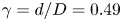$\gamma = d/D = 0.49$. The test section was modular so that its length could be extended. For the reported results, it comprised four consecutive parts, each 1.5 m long, so that the total length was $L\approx 320D_h$. Each test section part consisted of an inner and an outer glass tube, which were joined with those in the adjacent parts by machined plastic couplings. Each inner tube coupling was held in place by two vertical stainless steel wires, 0.3 mm in diameter, inserted through small holes in the outer tube coupling and kept taut by guitar tuning keys, which allowed a fine adjustment of the eccentricity. The eccentricity of each inner coupling was measured with a precision pin, which was inserted through the outer tube coupling for the measurements and retracted for the tests. Glass viewing tanks, filled with water, were fitted at several locations along the test section to permit optical access to the flow without significant distortion due to light refraction. The water was seeded with polyamide microspheres (Dantec Dynamics), having a mean diameter of 20 mm and a specific gravity of $1.03$.

Figure 1. Schematic diagrams of (a) the experimental apparatus and (b) its annular cross-section; the $x$-axis starts at the trumpet exit and is normal to the plane shown. The eccentricity is defined as $e=2\Delta y/(D-d)$.

The flow rate was measured using a calibrated ultrasonic flowmeter (Omega FDT-31). The test section Reynolds number was computed as

(2.1)\begin{equation} Re=\frac{U_b D_h}{\nu} , \end{equation}

where $U_b$ is the bulk velocity and $\nu$ is the kinematic viscosity of the fluid at the temperature of each test, measured with a thermistor inside the inlet tank, which varied from $21^{\circ }$ to $23^{\circ }$. The largest achievable Reynolds number was 12 000 and the estimated uncertainty of $\textit {Re}$ was at most 5 %. The uncertainty of the eccentricity was at most $0.05$. The standard deviation of the velocity fluctuations at the exit of the trumpet was at most 3 % of the local mean speed.

A two-component laser Doppler velocimeter (LDV; Dantec Dynamics, Fibre Flow 2-D LDV with a 160 mm focal length and a BSA F50 signal processor) was used for time-resolved measurements of the streamwise $U$ and cross-flow $W$ velocity components. Measurements were performed mainly at mid-gap between the inner and outer tubes, at the streamwise locations listed in table 1. Depending on the Reynolds number and eccentricity, the data rate varied from a few Hz to about 100 Hz. The velocity power spectral densities (PSDs) $E_{u}$ and $E_w$ were computed using the sample-and-hold method. This method cannot resolve accurately the PSD for frequencies greater than $2{\rm \pi}$ times the averaged particle data rate (Albrecht et al. Reference Albrecht, Damaschke, Borys and Tropea2003), so the range above this threshold was disregarded. Spectra were ensemble averaged over intervals 5 to 80 s long, depending on the conditions. The continuous wavelet transform, computed using the complex Morlet wavelet in the PyWavelets package (Lee et al. Reference Lee, Gommers, Waselewski, Wohlfahrt and O'Leary2019), was used to investigate the presence and frequency of quasi-periodic motions.

Table 1. Streamwise locations of measurements; positions 1, 2 and 3 were $10D_h$ upstream of the first three tube couplings and position 4 was $30D_h$ upstream of the test section discharge.

Flow visualisation was performed by observation of fluorescent dye injected isokinetically at mid-gap via a hypodermic needle inserted through the outer tube coupling. We verified that dye streak oscillations due to GI were not noticeably altered when passing from one section to another. This, together with LDV measurements closely downstream of the supporting wires and tube couplings, are deemed to be sufficient evidence that these devices did not significantly disturb the flow as far as GI was concerned.

2.2. Computational procedures

As a complement to the experimental study, numerical simulations of time-dependent, laminar flow were performed using the open source finite volume code OpenFOAM V6. The momentum and continuity equations were solved using the PISO algorithm. The equations were normalised by the hydraulic diameter $D_h$ of the channel and the bulk velocity $U_b$. All numerical schemes used were of second order, implicit in time and centred in space. The maximum Courant number was kept below 0.5; the resulting time step was between one and two orders of magnitude smaller than the period of any observed flow fluctuations. Pressure was fixed to zero at the outlet and a zero-gradient condition was imposed on all other boundaries. At the inlet, a uniform parallel flow having a velocity $u=U_b$ was imposed. In order to match as much as possible the experimental conditions, three-dimensional (3-D) velocity fluctuations generated by a pseudo-random number generator were superimposed to the inlet velocity. The standard deviations of these fluctuations were $0.02U_b$ for the streamwise velocity component and $0.01U_b$ for the two transverse components.

The mesh was generated with the open source software Gmsh (Geuzaine & Remacle Reference Geuzaine and Remacle2009). A representative mesh, consisting of hexahedral elements, is shown in figure 2 for $e=0.3$. The channel length was $330D_h$. Mesh dependence simulations were first performed in steady state, for $e=0.5$ and $\textit {Re}=500$, to determine the appropriate cross-sectional mesh density. A mesh having 3500 quadrangles in the cross-section was selected, as it produced a fully-developed velocity field that was essentially identical (within 0.3 %) to the one obtained with a mesh having 30 % more elements. The numerical solution of the base flow was validated by comparison to the theoretical solution by Snyder & Goldstein (Reference Snyder and Goldstein1965), with which it was found to be in excellent agreement.

Figure 2. Cross-section of the mesh used for the case with $e=0.3$; the shown elements were extruded in the streamwise direction to make the 3-D mesh; the detail shows the mesh near the inner wall.

The cross-sectional mesh was extruded in the streamwise direction to form prismatic elements with a uniform length $\Delta x$. This length was chosen following an additional mesh dependence study, this time for a time-dependent solution, from which we determined the GI frequency and wavelength $\lambda$ for different combinations of $\textit {Re}$ and $e$. For cases with $\lambda /D_h > 10$, which typically corresponded to flows with $\textit {Re}<1300$, we determined that the value $\Delta x = D_h$ provided sufficient accuracy. For cases with $\lambda /D_h < 10$, we used the value $\Delta x =0.5 D_h$. Simulations performed with meshes having half the value of the chosen $\Delta x$ gave comparable estimates (within 5 %) of the GI frequency and wavelength. A typical mesh had between 1.2 and 2.4 million elements.

3. Critical Reynolds number

The critical Reynolds number $\textit {Re}_c$ for each fixed $e$ was determined as the lowest $\textit {Re}$ value for which quasi-periodic cross-flow oscillations could be detected at position 4. The presence of such oscillations was confirmed by two independent methods: first, by observation of lateral motions of dye streaks injected at mid-gap with dye through a needle; and, second, by the detection of a peak in the cross-flow velocity spectrum, measured by LDV with the needle removed. Both methods gave comparable values, which are plotted in figure 3 for the entire range of eccentricities.

Figure 3. Critical Reynolds number for gap instability in eccentric annuli with $\gamma =0.5$.

The trends and the values of the present results are generally consistent with those obtained by Moradi & Tavoularis (Reference Moradi and Tavoularis2019) via a linear stability analysis at very small $e$ as well as the measurements by Choueiri & Tavoularis (Reference Choueiri and Tavoularis2015) for larger $e$, also shown in figure 3. One may note that the presently found $\textit {Re}_c$ for the case with $e=0.7$ was measurably lower than the value reported by Choueiri & Tavoularis (Reference Choueiri and Tavoularis2015). This difference is attributed to the fact that the present test section was much longer than the one in the previous study, thus allowing observation of GI onset at a lower $\textit {Re}$, but further away from the origin than it was possible in the previous study. A much stronger demonstration of the importance of channel length is provided by the case with $e=0.5$, for which, unlike the present apparatus, the test section of Choueiri & Tavoularis (Reference Choueiri and Tavoularis2015) was apparently insufficiently long for GI to become detectable in laminar flow. When applying the same logic to the present results, it becomes evident that one must consider the possibility that the presently reported experimental values of $\textit {Re}_c$ may be somewhat larger than the ideal values, which would presumably be measured in an infinitely long channel with the use of an experimental technique that has an infinite resolution, namely, at conditions that are impossible to meet in the laboratory.

Besides the experimental investigations, we have also determined the critical Reynolds number for GI by conducting numerical simulations of laminar flows in the same geometry for $e=0.5$, 0.3 and 0.1 and for $10 \leqslant \textit {Re} \leqslant 2000$. These have a much higher resolution than the experimental studies and permit the investigation of much longer channels. We have even employed the streamwise-periodic boundary condition to simulate numerically laminar flows in infinitely long channels (§ 8). Our simulations of the $e=0.5$ case have shown that quasi-periodic velocity fluctuations became detectable numerically at a Reynolds number that was close to the experimentally obtained $\textit {Re}_c$. In contrast, in the $e=0.3$ and 0.1 cases, the numerically obtained values of $\textit {Re}_c$ were significantly smaller than the experimental ones (figure 3). This apparent discrepancy between numerical and experimental estimates of $\textit {Re}_c$ can be resolved by consideration of the amplitude of cross-flows at mid-gap when $\textit {Re} \approx \textit {Re}_c$. Let us consider, for example, the $e=0.1$ case. The amplitude of cross-flows in the numerical study at $\textit {Re}_{c,{comp}} \approx 300$ was of the order of $10^{-6}U_b$, a value that is several orders of magnitude smaller than the experimental resolution. The amplitude of cross-flows in the experimental study at $\textit {Re}_{c,{exp}} \approx 1700$ was approximately $0.022U_b$. Such a cross-flow amplitude was observed in the numerical simulation of the $e=0.1$ case for $\textit {Re}'_{c,{comp}}=1600$ (a prime indicates the Reynolds number of a simulation that has a cross-flow amplitude that is comparable to the experimental value), i.e. a value that is only slightly lower than $\textit {Re}_{c,{exp}}$. For $e=0.3$, we also observed that $\textit {Re}'_{c,{comp}}$ was significantly larger than $\textit {Re}_{c,{comp}}$, whereas, for $e=0.5$, $\textit {Re}'_{c,{comp}} \approx \textit {Re}_{c,{comp}}$. It may further be noted that removing all turbulence from the inlet boundary condition did not affect our estimates of $\textit {Re}_{c,{comp}}$, but slightly increased the ones for $\textit {Re}'_{c,{comp}}$.

In conclusion, we consider the reported experimental values of $\textit {Re}_c$ to be reliable estimates of the onset of robust, albeit not necessarily dominating, GI and speculate that low-amplitude GI may be present at lower $\textit {Re}$, as suggested by our simulation results.

4. Streamwise development of gap instability

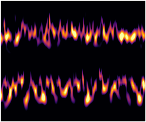
The PSD of the cross-flow velocity measured at different streamwise locations is plotted in figure 4, both for $e=0.3$ and different Reynolds numbers (top plots), and for $\textit {Re}=4000$ and different eccentricities (bottom plots). The occurrence of GI is indicated by a clear and dominant peak in the PSD, whereas the absence of such a peak indicates that GI has not occurred or is too weak to be detectable with the available means.

Figure 4. Power spectral density of the cross-flow velocity component at four different streamwise locations.

First, let us examine the cases with $e=0.3$, for which our experimental estimate was $\textit {Re}_c\approx 600$. In the ‘subcritical’ case with $\textit {Re}=520$, no GI was observed in the entire test section. In the slightly supercritical case with $\textit {Re}=630$, GI was observable only at position 4. As $\textit {Re}$ increased to 710, GI also became observable at position 3 and, following a further increase to 2000, GI was observable at positions 2, 3 and 4, although still not at position 1. One may further observe that, for a fixed position, the energy associated with GI (i.e. the area under the peak) increased with increasing $\textit {Re}$. Similar observations were made for other eccentricities for flows in the range $\textit {Re}\lesssim 2000$.

Next, let us examine the cases with $\textit {Re}=4000$, which is a value considerably larger than the corresponding $\textit {Re}_c$ for all eccentricities. A very prominent observation is that the energy of cross-motions is an order of magnitude larger for the $e=0.5$ case than for any case with a lower $e$. Another general observation is that, at position 1, GI was clearly observable only for the $e=0.5$ case and, even there, its amplitude was much smaller than further downstream. For lower eccentricities, velocity signals at position 1 were manifestly still dominated by inlet turbulence, which may have obscured the detection of GI. Such a statement is supported by our numerical simulations, which, when performed without any inlet turbulence, generally revealed the presence of a (very mild) peak at a location as close as $10D_h$ to the channel entrance. In contrast, when specifying a 2 % inlet turbulence as part of the boundary conditions, we were sometimes not able to discern a spectral peak until much further downstream, e.g. at $x \approx 150D_h$ for the $e=0.1$, $\textit {Re}=900$ case. Finally, in all cases shown in figure 4, in which there was a clear peak at position 2, the peak frequency somewhat decreased over some distance and reached a nearly constant value at positions 3 and 4.

At slightly supercritical conditions, one may plausibly anticipate that gap instability would occur intermittently, a condition that cannot be elucidated by the shape of velocity spectra alone. It is also reasonable to expect that this intermittency would decrease with increasing distance from the inlet. To address these issues, we examined time histories of the velocity along the channel. Figure 5 shows representative time histories of both the streamwise and the cross-flow velocity components for the case $e=0.5$, $\textit {Re}=520$ and for positions 2, 3 and 4. For this case, the experimental $\textit {Re}_c$ was approximately 400. One may first notice that all time histories contained intervals with strong quasi-periodic oscillations, during which the local time-averaged streamwise velocity $\bar {U}$ was high, interspersed with intervals of much weaker activity, during which $\bar {U}$ was low. These observations are consistent with the fact that cross-flows associated with GI transport high-speed fluid from the wide gap into the narrow gap region. The duration of the active intervals increased from roughly 45 % of the total time interval at position 2 to about 72 % at position 3 and reached 93 % at position 4. A visible difference between the waveforms of the streamwise and cross-flow components during active intervals is that the latter appeared to have a single dominant frequency, whereas the former was more complex and appeared to have a higher frequency content. This difference is illustrated clearly by the corresponding PSD, also shown in figure 5: all cross-flow PSD had a single strong peak at a frequency to be denoted as $f_p$, whereas the streamwise PSD had two distinct peaks, one at $f_p$ and another at $2f_p$. The single peak of the cross-flow PSD is confidently attributed to the passage of a pair of counterrotating vortices on either side of the narrow gap. The same mechanism is obviously responsible for the peak of the streamwise velocity PSD at $f_p$ (Choueiri & Tavoularis Reference Choueiri and Tavoularis2014); an explanation for the peak at $2f_p$ will be given in § 5.3.

Figure 5. (a) Time history of the dimensionless streamwise and cross-flow velocity components at positions 2 (i), 3 (ii) and 4 (iii) for $e=0.5$, $\textit {Re}=520$; (b) PSD of the corresponding streamwise (i) and cross-flow (ii) velocity fluctuations.

Lastly, despite the fact that, between position 2 and position 4, the amplitude of the peak in $E_w$ increased by a factor 2, the maximal amplitude of $W/U_b$ did not change noticeably. This indicates that the streamwise increase in spectral energy corresponding to GI activity was not due to the strengthening of cross-flows but to the increase of the portion of the time that was occupied by quasi-periodic motions.

The main observations made in this section may be summarised as follows.

1. (i) For a fixed $e$, the GI onset took place at a location that moved upstream with increasing $\textit {Re}$. For $\textit {Re} \gg \textit {Re}_c$, however, the onset location did not vary measurably with $\textit {Re}$.

2. (ii) In general, for a fixed $\textit {Re}$, GI was observed closer to the inlet at high eccentricity ($e\geqslant 0.5$) than at low eccentricity ($e\leqslant 0.3$). For instance, for $\textit {Re}=4000$, GI was observed at $70D_h$ for $e=0.5$, but only at $150D_h$ for $e\leqslant 0.3$.

3. (iii) Once GI was triggered, its energy increased and its frequency decreased downstream, reaching a nearly constant level at some distance from the inlet. For $\textit {Re} \gg \textit {Re}_c$, this distance typically corresponded to position 3 ($x\approx 230D_h$).

4. (iv) As the streamwise distance increased, the observed quasi-periodic motions across the gap became less intermittent and their amplitude became more uniform. Such effects were observed under all conditions, but were particularly noticeable for slightly supercritical conditions.

5. ‘Fully developed’ gap instability

Based on the results presented in §§ 3 and 4, one may characterise GI to be ‘fully developed’ starting from the location where its energy and dominant frequency essentially reach asymptotic levels. In most cases discussed, such requirements were met at position 4. In cases, however, in which $\textit {Re}$ slightly exceeded $\textit {Re}_c$, it seems logical that, had the channel been longer, the cross-flows might have continued to grow somewhat before settling. Similarly, in cases with $\textit {Re}$ slightly lower than $\textit {Re}_c$, GI might have been triggered at some downstream location, which would entail a (presumably small) reduction of $\textit {Re}_c$.

5.1. The effects of eccentricity and Reynolds number

The power spectral density (PSD) of the cross-flow velocity component at position 4 is shown in figure 6 for eccentricities in the range $0 \leqslant e \leqslant 0.5$ and Reynolds numbers in the range $500 \leqslant \textit {Re} \leqslant 9100$. These results are unique in the literature and allow one to make the following original observations.

1. (i) GI in a long channel occurs over a specific range of $\textit {Re}$ for $0.05 \lesssim e \lesssim 0.5$; this complements previous observations of GI occurrence in a much shorter channel, but only for higher eccentricities ($e \gtrsim 0.5$).

2. (ii) For a fixed Reynolds number, the energy within the bandwidth of the spectral peak (namely, the amplitude of cross-gap fluctuations and the portion of the time they were uninterrupted) generally decreases with decreasing eccentricity.

3. (iii) Among the cases shown in the plots, the critical Reynolds number for GI is lowest for $e = 0.5$ and increases with decreasing $e$. For example, for $\textit {Re} = 500$, the PSD has a sharp peak when $e = 0.5$, a much milder peak when $e = 0.3$ and no peak at all for lower $e$.

4. (iv) For $e=0.5$, the PSD had sharp peaks for all values of $\textit {Re}$ considered, including 9100, which corresponds to fully turbulent flow. Rather unexpectedly, for $e=0.3$, 0.2 and 0.1, no spectral peaks were observable for $\textit {Re} \geqslant 6100$, although such peaks were present at lower $\textit {Re}$. For low $e$, strong evidence of GI was thus only found in laminar, and possibly transitional, flows, but not in fully turbulent ones. This issue will be discussed in more detail in the next subsection.

Figure 6. Power spectral density of the cross-flow velocity component for selected eccentricities and Reynolds numbers.

Despite the fact that $\textit {Re}=2000$ is close to the transitional $\textit {Re}$ in concentric annuli, the observed spectral peak for the $e=0.1$, $\textit {Re}=2000$ case is attributed to GI and not to some transition mechanism. This is supported experimentally by the observation that, although the peak for the $e=0.1$ case was weaker than the peaks in the $e \geqslant 0.2$ spectra, it appeared to be very distinct in light of the absence of such a peak in the $e\lesssim 0.05$ spectrum. Strong evidence for the presence of GI in the $e=0.1$, $\textit {Re}=2000$ case is provided by our computational study of this case, which identified quasi-periodic structures with characteristics very similar to the ones observed at higher $e$. Additional computational findings regarding GI in low-$e$ flows will be presented in § 8.

5.2. On the absence of gap instability in low-$e$–high-$\textit {Re}$ flows

Figure 7(a) provides quantitative support for the previous observation that, in the range $e \lesssim 0.5$ and for a fixed $\textit {Re}$, the energy of cross-flows associated with GI generally decreases with decreasing $e$. This energy was evaluated as the integral of the cross-flow spectrum in the peak region (typically for $f\leqslant 5$ Hz) and was normalised by $U_b^2$. Figure 7(b) further supports this and other previous observations. First, when $\textit {Re} \gg \textit {Re}_c$, GI is much stronger in high-$e$ channels than in low-$e$ ones. Second, for $e \lesssim 0.3$, GI is triggered only within a range of $\textit {Re}$ and disappears when $\textit {Re} \gtrsim 4000$. In contrast, for $e = 0.5$ and 0.7, GI was found to be strong even for the largest examined $\textit {Re}$ of 12 000. The near-constancy of this energy over a long range of $\textit {Re}$ for $e = 0.7$ seems to indicate that this property could maintain the same value at indefinitely large $\textit {Re}$. Results for the $e=0.7$ case are consistent with the fact that GI was observed at much higher $\textit {Re}$ in other geometries having very small gaps (Meyer & Rehme Reference Meyer and Rehme1994; Guellouz & Tavoularis Reference Guellouz and Tavoularis2000) and in tightly-packed rod bundles (e.g. Möller Reference Möller1991; Wu & Trupp Reference Wu and Trupp1993; Krauss & Meyer Reference Krauss and Meyer1998). On the other hand, the observed downward trend for the $e=0.5$ curve suggests that the instability may also decay to an undetectable level at some higher $\textit {Re}$ (this is consistent with the LES studies of Merzari & Ninokata (Reference Merzari and Ninokata2009) for the $e=0.5$ case; these authors noted the presence of periodic coherent structures for $\textit {Re}=3200$, but not for $\textit {Re}=27\,000$); this trend thus appears to be intermediate between the trends of the $e=0.7$ and $e\leqslant 0.3$ cases.

Figure 7. Normalised energy of mid-gap cross-flows as a function of eccentricity (a) and Reynolds number (b). The gap instability (GI) energy was computed by integrating the power spectral density (PSD) in the peak region.

In view of the fact that, at low $e$, $\textit {Re}_c$ increases with decreasing $e$, it becomes evident that the range of $\textit {Re}$ over which GI can be observed diminishes with decreasing eccentricity. For the lowest achieved $0 \lesssim e \lesssim 0.05$, this range was reduced to $2500 \lesssim \textit {Re} \lesssim 4000$. This observation accentuates the complexity of the gap instability mechanism(s). It also underscores the difficulty in detecting GI in the limit of vanishing eccentricity.

Another important observation in figure 7 is that the cross-flow energy for $e=0.2$ and 0.3 dropped by nearly an order of magnitude as $\textit {Re}$ was increased from 2000 to 4000, which presumably coincides with the onset of transition somewhere in the annular channel. If one considers that (Merzari & Ninokata Reference Merzari and Ninokata2009) transition may first occur in the wide gap of the annulus, one may speculate that, under such conditions, the flow could be laminar in the narrow gap and transitional or turbulent elsewhere. A laminar profile would have a relatively large velocity peak at mid-gap, whereas a turbulent profile would have a comparatively smaller peak, which would diminish the azimuthal velocity gradient, thus weakening the source of instability.

The absence of a strong peak in the cross-flow PSD under turbulent conditions does not necessarily mean that GI was never triggered under such conditions. One may also examine the possibility that GI was occasionally triggered, but was quickly suppressed by conventional turbulence or remained too weak to be easily detectable. We investigated such possibilities using the continuous wavelet transform, which detected coherent events as a function of time. An example of a wavelet plot, obtained for $e=0.1$ and $\textit {Re}=6000$, is shown in figure 8. One may observe the presence of some relatively short intervals of time displaying a high wavelet activity in the frequency range where GI is expected to occur, which in this case was $f\sim 1\ \textrm {Hz}$. When computing the PSD by considering such a localised time period, one can actually observe a clear peak. Even though such observations were not reproducible in a consistent manner, they seem to indicate that GI is occasionally triggered in high-$\textit {Re}$-moderate/low-$e$ flows, namely, for $e \lesssim 0.3$ and for $\textit {Re} \gtrsim 5000$, but it is weak and highly intermittent, so that it is mostly obscured by turbulence.

Figure 8. Wavelet transform of the cross-flow velocity component for $\textit {Re} = 6000{}$, $e = 0.1$ (a); zoomed portion of the wavelet plot (b); two realisations of the corresponding velocity spectrum computed using different time intervals, namely for the 600 s full signal and the 90 s zoomed portion (c).

5.3. An explanation for the two peaks in the streamwise velocity spectrum

The measured streamwise velocity spectra that were presented in figure 5 for $e=0.5$ and $\textit {Re}=520$ showed two distinct peaks, one at $f_p$ and another at $2f_p$. The spectral content of $E_u$ was analysed by examining numerical results for the case with $e=0.5$ and $\textit {Re}=700$, for which the flow pattern was comparable to that corresponding to the previously cited figure. We found that, in the narrow gap region, streamwise velocity fluctuations generated by two successive vortices were positively correlated for positions near the channel symmetry plane, and that the correlation weakened and became negative towards the wide gap. These correlations can be explained by the self-evident expectation that consecutive vortices have nearly the same shape, when shifted streamwise and reflected on the geometric plane of symmetry (see also § 7). In contrast, cross-flow fluctuations were found to be negatively correlated nearly everywhere in the cross-section. These observations are supported by the three plots in figure 9, in which $E_u$ and $E_w$ are plotted, respectively, at mid-gap and at two other locations away from it. At mid-gap (left plot), only one strong peak was observable in $E_u$, at a frequency equal to $2f_p$. For a location slightly to the side of mid-gap (middle plot), $E_w$ did not change measurably but $E_u$ developed a second measurable peak at $f_p$. Further away from the narrow gap (right plot), the peak at $2f_p$ nearly vanished, whereas the one at $f_p$ became dominant. The findings and trends observed in the numerical simulations are generally consistent with our experimental results and observations. For example, in the experiments, a peak at $2f_p$ was indeed only observable near the channel symmetry plane, although we noticed that the amplitude of this peak relative to the one at $f_p$ was very sensitive to the azimuthal location. Hence, the presence of the two $E_u$ peaks in figure 5 was most probably due to the fact that measurements were not performed exactly at mid-gap, but at a location slightly offset towards either side of the annulus.

Figure 9. Numerical estimates of the power spectral density (PSD) of the streamwise and cross-flow velocity ($E_u$ and $E_w$, respectively) at three different cross-sectional locations, which are indicated by red dots; $e=0.5$, $\textit {Re}=700$; $x/D_h=250$.

6. Strouhal number and gap instability modes

The dominant dimensionless frequency of cross-flows is represented by the Strouhal number ${\textit {St}}= f_p d / U_b$, where, as mentioned previously, $f_p$ is the frequency of the cross-flow PSD peak and $U_b$ is the bulk velocity. In most cases considered, the PSD had a clear single peak, which provided an unambiguous estimate of $f_p$. In some cases, however, the peak was broadband, thus introducing uncertainty in the estimate of ${\textit {St}}$. To obtain ${\textit {St}}$ in, as much as possible, ‘fully developed’ flows, we determined $f_p$ at position 4, for various eccentricities and Reynolds numbers. Based on these results, which are plotted in figure 10, we can make the following observations and comments.

1. (i) The range of $\textit {Re}$ for each $e$ is bounded from below by the corresponding $\textit {Re}_c$.

2. (ii) For the $e=0.7$ and 0.5 cases, there is no upper bound for the $\textit {Re}$-range. In contrast, for $e \leqslant 0.3$, there is an upper bound in the vicinity of 4000, which indicates that GI was not observed clearly in turbulent, and possibly transitional, flows. The presence of such an upper bound has already been documented by figure 7.

3. (iii) For all $e$, ${\textit {St}}$ increases monotonically up to some $\textit {Re}$. In this $\textit {Re}$ range, ${\textit {St}}$ increases monotonically with decreasing $e$.

4. (iv) For $e=0.7$, ${\textit {St}}$ settles at approximately 0.09 at $\textit {Re} \approx 4000$.

5. (v) For $e \leqslant 0.5$ the rise in ${\textit {St}}$ is followed by a drop, which becomes more abrupt as the eccentricity decreases. For $e=0.5$, the rate of decrease is mild, whereas, for $e\leqslant 0.3$, ${\textit {St}}$ suddenly drops to $\approx 0.065$ for $\textit {Re}\approx 2900$ and maintains this value for $2900 \lesssim \textit {Re} \lesssim 4000$.

6. (vi) The intense drop observed for $e\leqslant 0.3$ is preceded by a range with large variations of ${\textit {St}}$, which may be attributed to a high sensitivity of GI characteristic to the Reynolds number.

7. (vii) For $e=0.3$, $\textit {Re}=2900$, two values are plotted for ${\textit {St}}$, corresponding to the two peaks marked by circles in the power spectrum of figure 6.

8. (viii) The Strouhal number values in the simulations are generally lower than the corresponding experimental ones, but they follow similar trends: ${\textit {St}}$ increases for decreasing $e$ and for increasing $\textit {Re}$.

Figure 10. Strouhal number of gap instability as a function of the Reynolds number (a) and eccentricity (b). Solid and dashed lines in the right plot refer to the primary and secondary GI modes, respectively; dotted lines connect simulation results.

Results obtained for $e=0.7$ are consistent with earlier findings in annular channels (Choueiri & Tavoularis Reference Choueiri and Tavoularis2015) and rod bundles (Möller Reference Möller1991; Meyer Reference Meyer2010), namely that ${\textit {St}}$ increases with $\textit {Re}$ in laminar flows and settles at an approximately constant value in turbulent flows. The same observation also seems to apply to the case with $e=0.5$, but not to cases with lower eccentricities. To elucidate this difference, we may reconsider the PSD shown in figure 6. For $e=0.5$, the GI peak broadened as $\textit {Re}$ was increased to 1300 and remained broad at higher $\textit {Re}$. For $e\leqslant 0.3$, however, this peak became noticeably narrower as $\textit {Re}$ was increased from 2900 to 4000, which may signify that one or more modes disappeared or became attenuated. This issue will be further investigated in the following by observation of wavelet plots of the mid-gap cross-flow velocity component.

Let us start by comparing the three wavelet plots for $e=0.5$, corresponding, respectively, to $\textit {Re}=2000$, 4000 and 11 500 and shown in figure 11. A first general observation is that the instantaneous dominant frequency, identified by large values of the wavelet coefficient, wandered in time. Such frequency wandering, which was noticed for all eccentricities and Reynolds numbers in both experiments and simulations, could not be accounted for by fluctuations of the flow rate and has already been observed by de Melo et al. (Reference de Melo, Goulart, Anflor and dos Santos2017) for the turbulent flow inside a compound rectangular channel. Figure 11 further shows that the width of the wavelet band, bounded by the two white dashed lines in the figure, increased considerably while $\textit {Re}$ was increased from 2000 to 4000, but then decreased at higher $\textit {Re}$ to a level that was comparable to the one observed for $\textit {Re}=2000$. A widening of the wavelet band was also noticed for $e\leqslant 0.3$ and $\textit {Re}\approx 2900$, but was not observed for $e=0.7$. These effects are illustrated in figure 12, where the ratio $f_h/f_l$ of the two frequencies bounding the GI wavelet band is plotted as a function of the Reynolds number for four different eccentricities. For $e=0.3$, 0.2 (not shown) and 0.1, a sharp peak on the ratio separates data for $\textit {Re}\leqslant 2000$ from those for $\textit {Re}=4000$; a similar peak of this ratio can also be observed for $e=0.5$ at somewhat higher $\textit {Re}$, but the data for $e=0.7$ show no peak.

Figure 11. Continuous wavelet transform (a,b,c) and power spectral density (PSD) (d,e,f) of the mid-gap cross-flow velocity component for $e=0.5$ and various $\textit {Re}$. The abscissa range of each wavelet plot was set at approximately $100/f_p$, although the PSD were computed with the corresponding 600 s full signal. The ordinates of different plots were shifted, but their range was kept at one order of magnitude. Wavelet coefficients are normalised by their corresponding maximum and values lower than 30 % were filtered out to avoid clutter.

Figure 12. Ratio $f_h/f_l$ of the upper and lower frequency bounds of the wavelet band for various eccentricities and Reynolds numbers.

Now, let us consider the wavelet plot shown in figure 13 for the intermediate case having $\textit {Re}= 2900$ and $e=0.3$. In contrast to previous ones, this wavelet plot shows the presence of two modes having well separated frequencies and thus resulting in two distinct spectral peaks. The figure also shows that these modes did not occur simultaneously but rather alternated in time, and that the frequency of each mode wandered somewhat over time. (By ‘mode’ here we do not refer to a single frequency, but rather to frequencies in the range $[f_l,f_h]$.) It should be noted that the frequency ratio plotted in figure 12 for this case was evaluated by only considering the width of the more energetic among the two wavelet bands (namely the one at higher frequencies), and thus does not include the large frequency interval separating the two spectral peaks. We may then hypothesise that the high-frequency mode is the one that was found to be dominant in laminar flow for all $e$, whereas the low-frequency mode corresponds to one that was triggered at intermediate $\textit {Re}$ for $e\lesssim 0.3$, and possibly for $e=0.5$. The validity of this hypothesis is demonstrated in figure 10(b), where it is evident that the higher of the two observed ${\textit {St}}$ for $e=0.3$ and $\textit {Re}=2900$ follows the trend that was observed for $\textit {Re}=1300$ and $\textit {Re}=2000$, whereas the lower ${\textit {St}}$ follows the trend observed for $\textit {Re}=2900$ and $\textit {Re}=4000$, which was very different from the previous one. Mode switches also seemed to have occurred for $e=0.1$ and $e=0.2$ at slightly lower $\textit {Re}$ as depicted by large ${\textit {St}}$ variations in figure 10. Considering the previous analysis of figures 11 and 12, we may further conjecture that the mode in laminar flow is of the same type as the one occurring for $e=0.5$ under fully turbulent conditions and for $e=0.7$ for the entire considered range of $\textit {Re}$, which includes both laminar and fully turbulent regimes. To distinguish this from other motions, we may refer to it as the ‘primary’ GI mode. For some ranges of $\textit {Re}$ in the same eccentricity range ($e\lesssim 0.3$), this primary mode seems to coexist with a lower-frequency, ‘secondary’ mode. This secondary mode becomes dominant for $\textit {Re}\gtrsim 2900$, but either vanishes or is too weak and intermittent to be detectable in fully turbulent flow. One is reminded that, as $\textit {Re}$ exceeded this approximate bound of 2900, both ${\textit {St}}$ and the GI energy dropped sharply for the low-$e$ cases (figures 7 and 10). The concurrent presence of two modes at low eccentricities follows our previous postulation that the flow in the wide gap underwent intermittent transition to turbulence, while the flow in the narrow gap remained laminar. In high-$e$ flows, the primary mode may be too strong for any other secondary mode to grow or become observable.

Figure 13. Continuous wavelet transform (a) and power spectral density (PSD) (b) of the cross-flow velocity component for $\textit {Re}=2900$, $e=0.3$.

Lastly, for $e=0.5$ and $\textit {Re}=4000$, the local increase of the frequency ratio observed in figures 11 and 12 suggests that the secondary mode may have alternated with the primary one in this case as well, but without either of the modes being dominant. Because, however, the spectrum had a single broad peak, we cannot assert with confidence that multiple modes were present. As stated previously, the case with $e=0.5$ appears to be a borderline eccentricity, which shares some characteristics with low-$e$ flows and others with high-$e$ flows, at least as far as GI is concerned.

7. An improved vortex street model

The mechanism of gap instability has been associated with the formation of a ‘gap vortex street’, an idealised, 2-D model of which was proposed by Möller (Reference Möller1991) and refined by Krauss & Meyer (Reference Krauss and Meyer1998). This model is consistent with some of the main experimental and numerical findings, but cannot explain some other observations. Besides, it is self-evident that gap vortices are not isolated and cannot be 2-D, while confined in an annular channel. In this section, we present a more realistic model of a gap vortex street, which is based on our numerical results and is consistent with the experimental evidence.

Figure 14(a) shows a snapshot of a computed, fully developed, gap vortex street for a representative case with $e=0.5$ and $\textit {Re}=700$. The vortices (coherent structures) were identified by the $Q$ criterion (Jeong & Hussain Reference Jeong and Hussain1995), namely as isosurfaces of the parameter $Q=(\lVert \boldsymbol{\Omega} \rVert ^2 - \lVert \boldsymbol{\mathsf{S}}\rVert ^2)/{2}$, where $\boldsymbol{\Omega}$ and $\boldsymbol{\mathsf{S}}$ are, respectively, the anti-symmetric (rotation) and symmetric (strain rate) parts of the velocity gradient tensor. The isosurfaces shown in this figure correspond to $Q= 0.15 U_b^2/D_h^2$ and were coloured red or blue to denote, respectively, a positive or negative sign of the azimuthal component (namely, the one in the $\theta$ direction, which has been defined in figure 1) of the vorticity vector. Each of the presented isosurfaces of $Q$ is wrapped around the core of the channel, it is elongated strongly in the streamwise direction, and it is continuous on one side of the core and broken on the other side. The shape of these isosurfaces indicates that gap vortices, when adequately developed, may be roughly described as twisted, tilted and broken rings, which are asymmetric with respect to the geometric plane of symmetry. Each gap vortex is paired with a secondary, counterrotating vortex in the outer region of the wide gap (such secondary vortices were also observed by Chang & Tavoularis (Reference Chang and Tavoularis2012) in their simulations of turbulent flow in a rectangular annulus); these secondary vortices, which are driven by the main vortices in a manner similar to vortices in cavities, will not be discussed further. Successive gap vortices are both tilted and twisted in an opposite manner, but, in all cases, the vortex part in the narrow gap is downstream of the part in the wide gap. Consistent with the fact that vortex rings are tightly wrapped around the inner cylinder, a region where the azimuthal vorticity $\omega _\theta \approx -\partial u/\partial r$ is negative, all vortices rotate counterclockwise. In combination with the vortex tilting, this vortex orientation induces cross-flows between consecutive vortices that transport fluid across the gap from both sides of the inner cylinder, in a manner similar to the cross-flows produced by the Krauss/Meyer model.

Figure 14. Vortices identified numerically as isosurfaces of the parameter $Q$ for the case with $e=0.5$ and $\textit {Re}=700$. The streamwise axis was scaled down by a factor of two, so that the vortices were actually twice as long as they appear to be. In the 3-D view (a), the isosurfaces have been coloured according to the azimuthal vorticity component, whereas, in the side view (b), the colouring corresponds to the streamwise vorticity component. The solid arrow drawn on the side view marks the overall direction of the vorticity vector within the vortex on the front of the inner cylinder and the dashed arrow marks this direction behind the inner cylinder.

The twisting of the rings orients some vorticity in the streamwise direction, as illustrated in the bottom plot of figure 14, where isosurfaces are coloured according to the sign of the streamwise vorticity component. The sign of the streamwise vorticity alternates from one vortex to the next, thus clearly distinguishing consecutive vortices, which may be considered as pairs. This alternation of streamwise vorticity is essential for the generation of alternating cross-gap flows. In the figure, the red and blue arrows mark the approximate direction of the vorticity vector on the unbroken side of each vortex.

It is evident that the vortex patterns in annular channels are too complex to be captured by an all-encompassing, simple physical model. It is possible, however, to improve the 2-D model of Krauss & Meyer by idealising the gap vortex street as a sequence of oppositely tilted and twisted, interconnected vortex rings. Both models are illustrated schematically in the top sketch of figure 15. Although the previously presented isosurfaces of $Q$ are open at both ends (points $A$ and $B$ in figure 15), a careful inspection of isosurfaces corresponding to lower values of $Q$ indicated that each vortex splits at end $A$ into two branches: a branch that was connected to the downstream vortex, in a manner reminiscent of the streamwise vortex connections between von Kármán vortices in the wake of a cylinder, and a second branch that reconnected at another point of the original vortex, thus closing the ring; a similar branch connected end $B$ of each ring to the upstream vortex. An interconnected version of our model is proposed at the bottom of figure 15. This model is consistent with the observation that circulation in each fully developed vortex is stronger in the two gap regions than on the sides of the annulus, where the vortex splits into branches.

Figure 15. Sketches of fully developed gap vortices according to the Krauss & Meyer (Reference Krauss and Meyer1998) model and according to the present model. The sketch at the top shows idealised $Q$ isosurfaces, whereas the sketch at the bottom is a simplified version of the ‘interconnected rings’ model.

8. Vortex generation and development

The previous model describes the vortex street only at its fully developed state. The present simulations, however, allow us to describe the vortex street from its inception to its full development. $Q$-isosurfaces relatively close to the inlet, shown for a representative case in figure 16(a), illustrate that, in agreement with observations by previous authors (Choueiri & Tavoularis Reference Choueiri and Tavoularis2014; Moradi & Tavoularis Reference Moradi and Tavoularis2019), the vortices were not generated in the narrow gap, but rather on the two sides of the annulus. The vortex generation mechanism may be summarised as follows. The flow enters the annulus with a uniform velocity, but the growing, lower-velocity, wall layers occupy a larger portion of the narrow gap region than that of the wide gap region. As a consequence, fluid is displaced through the sides from the narrow gap towards the wide gap. This motion generates streamwise vorticity, which is strongest on the two sides of the channel core. As they evolve downstream, the vortical regions on the sides of the core become more elongated and intensified. At some distance from the inlet, they become unstable and break down into discrete vortices, which, at this immature stage, resemble the vortices in the 2-D model. (It is worth mentioning that streamwise vortical regions were also observed near the inlet for subcritical $\textit {Re}$, but they were stable and did not break down to discreet vortices. In some cases with $\textit {Re}\approx \textit {Re}_c$, especially in low-$e$ channels and when using the streamwise-periodic boundary condition, weak cross-flows were observable close to the inlet, but the flow stabilised further downstream.) The axes of these vortices get tilted, thus converting some streamwise vorticity to azimuthal vorticity, which, as vortices get convected downstream, generates cross-flow fluctuations with largest amplitude in the narrow gap. With further development, each vortex gets stretched into and around the narrow and wide gaps towards the other side of the core, where its ends split and reconnect to another part of the same vortex or a consecutive vortex. At this stage and beyond, the 2-D model fails to describe, even roughly, these vortices. Figure 16(a) illustrates that, for this case that has a moderate eccentricity, discrete vortices appear relatively close to the channel inlet and specifically at $x/D_h \approx 30$, whereas quasi-periodic cross-flows were observable as close to the inlet as at $x/D_h \approx 10$. For low eccentricities, however, we have already (§ 5.3) presented evidence that GI becomes first detectable much further downstream. For example, for $e=0.1$ and $\textit {Re}=2000$, vortices were first identified by the $Q$ criterion at $x/D_h \approx 230$. Despite the slowness in its activation, the laminar vortex generation mechanism for very low $e$ is the same as the one observed for the moderate and large $e$ cases. This is illustrated in figure 16(c), which shows that vortices that appear in the far downstream region for the case with $e=0.1$ and $\textit {Re}=2000$ have the same shape as vortices that appear in the near-inlet range for the case with $e=0.5$ and that, in both cases, the vortices are located on the side of the annulus. We have further performed streamwise-periodic simulations for the $e=0.1$ case and found that, given enough development time ($tU_b/D_h \approx 750$, which is equivalent to a distance of $750D_h$, if one assumes that the convection speed of the vortices is equal to $U_b$), the vortices eventually evolved into interconnected rings. These observations support our assertions that the same GI generation mechanism is present in laminar flows in channels with both small and moderate/large eccentricities and that the GI onset location depends on the values of $e$ and $\textit {Re}$ and may move very far downstream as $e$ decreases to small values. Lastly, simulations were also performed by imposing the fully-developed basic flow field at the inlet. It is interesting to note that such a condition did not impede the triggering of GI, but rather accelerated the vortex development process. As observed in figure 16(d), the inlet vortical regions were in this case barely observable and the discrete vortices were formed much closer to the inlet than in cases with the uniform inlet velocity.

Figure 16. Generation and streamwise development of a gap vortex street for (a,b) $e=0.5, \textit {Re}=700$ and (c) $e=0.1, \textit {Re}=2000$, as identified by the $Q$ criterion with 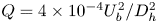$Q=4\times 10^{-4}U_b^2/D_h^2$; (d) same as (a), but obtained with the use of the fully-developed basic flow field as the inlet condition and $Q$ ten times lower.

To conclude this discussion, we would like to emphasise that vortices in eccentric annular channels were not always as well-defined as the ones shown in figures 14 and 16 and that the presence of such vortices is not a necessary condition for the existence of GI. In some cases, for example the case with $e=0.3$ and $\textit {Re}=1600$, we found that vortices that were generated by the GI mechanism broke down with distance, so that they were no longer identifiable by the $Q$ criterion; nevertheless, the presence of a distinct peak in the $w$ spectrum (not shown here) proved that the GI mechanism remained active beyond the location of vortex breakdown. In some other cases, vortices generated and broken down formed again further downstream; such a case, computed with the use of streamwise-periodic boundary conditions for $e=0.1$ and $\textit {Re}=1600$, is shown in figure 17. Furthermore, signs of vortex breakdown were also present in some experiments, as documented by the observation of dye streaks. In the range $0.3 \leqslant e \leqslant 0.7$, dye streaks had quasi-sinusoidal shapes when $1000 \lesssim \textit {Re} \lesssim 1300$, but, for higher $\textit {Re}$, they often broke down and got mixed with the surrounding fluid within $2D_h$ past the dye injection point. In general, for $e < 0.3$ or for $\textit {Re}_c \leqslant \textit {Re} \lesssim 1000$, quasi-periodic dye streaks were observable, but successive waves were rather irregular.

Figure 17. Isosurfaces of the $Q$ parameter, coloured as in figure 14 (bottom), for an example showing the breakdown and regeneration of vortices; $e=0.1$, $\textit {Re}=1600$, streamwise-periodic boundary conditions, $Q=0.01U_b^2/D_h^2$.