2. Basic equations

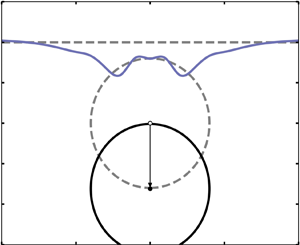
Consider the disturbances on the free surface of a fluid as a circular cylinder submerges underneath, as shown in figure 1. A Cartesian coordinate system is fixed with the $X$-axis along the unperturbed surface and the $Y$-axis passing through the centre of the circle, directed vertically upwards. The fluid is assumed to be inviscid, incompressible and initially at rest. The extension of the fluid is considered infinite in depth (negative $Y$ direction) and lateral extent (both $X$ directions). Also, surface tension effects are neglected.

Figure 1. Definition sketch with dimensional variables of the system. Transparent dashed lines indicate the initial state of the system. Solid lines indicate a later time $t$.

To non-dimensionalize all the variables, lengths have been scaled by the initial depth of the cylinder $H_0$, velocities by a characteristic motion speed $U_0$, time by $H_0/U_0$ and pressures by $\rho U_0^{2}$, where $\rho$ is the density of the fluid. Dimensional variables are denoted with upper-case letters, while their non-dimensional counterparts are lower-case. The non-dimensional radius $r = R/H_0$ is the size of the cylinder relative to its initial depth. With this in mind, references to the size of a cylinder made throughout will be referring to the $r$-value of the cylinder. Hence, one cylinder can be bigger than another while having a smaller radius $R_0$ if its initial depth $H_0$ is small enough to make its value of $r$ larger than the corresponding $r$ of the second cylinder. In essence, the size of the cylinder is representative of the distance to the free surface, with a larger cylinder being closer to the free surface than a smaller one.

The assumptions ensure the existence of a potential flow in the time-dependent fluid region $\varOmega (t)$. The motion of the cylinder, whose boundary is $\partial \varOmega _C$, is prescribed through the time functions $(x_c(t), y_c(t))$ that describe the position of the centre of the cylinder, with initial conditions $x_c(t=0)=0$ and $y_c(t=0)= -1$. The location of the free surface, denoted as $\partial \varOmega _F: y=\eta (x,t)$, must be computed as part of the solution. Under this formulation, the initial/boundary-value problem for the flow velocity $\boldsymbol {u}(x,y,t)$ and the pressure $p(x,y,t)$ is given by the following equations:

(2.1)$$\begin{gather} \boldsymbol{u}_t+(\boldsymbol{u}\cdot \boldsymbol{\nabla})\boldsymbol{u}+ \boldsymbol{\nabla}p=\lambda \boldsymbol{e}\quad \mbox{in}\ \varOmega(t), \end{gather}$$

(2.2)$$\begin{gather}\boldsymbol{\nabla}\boldsymbol{\cdot}\boldsymbol{u}=0,\quad \boldsymbol{\nabla}\times \boldsymbol{u}=0\quad \mbox{in}\ \varOmega(t), \end{gather}$$

(2.3)$$\begin{gather}\eta_t+u^{(x)}\eta_x=u^{(y)}, \quad p=0\quad \mbox{on}\ \partial \varOmega_F(t), \end{gather}$$

(2.4)$$\begin{gather}\left( \boldsymbol{u} -\boldsymbol{u}_c\right)\boldsymbol{\cdot} \boldsymbol{n}= 0 \quad \mbox{on}\ \partial \varOmega_C(t), \end{gather}$$

(2.5)$$\begin{gather}\eta \rightarrow 0 \quad \mbox{for}\ x \rightarrow \infty\ \mbox{on}\ \partial \varOmega_F(t), \end{gather}$$

(2.6)$$\begin{gather}\boldsymbol{u}\rightarrow 0 \quad \mbox{for}\ \sqrt{x^{2} +y^{2}} \rightarrow \infty\ \mbox{in}\ \varOmega(t), \end{gather}$$

(2.7)$$\begin{gather}\eta = 0 \quad \mbox{for}\ t=0\ \mbox{on}\ \partial \varOmega_F(t=0), \end{gather}$$

(2.8)$$\begin{gather}\boldsymbol{u}= 0 \quad \mbox{for}\ t=0\ \mbox{in}\ \varOmega(t=0). \end{gather}$$

Here $\boldsymbol {e}=[0,-1]$ is the unit vector in the direction of the gravity acceleration. The square of the inverse Froude number $\lambda =gH_0/U_0^{2}$ indicates the balance between gravitational and inertial forces. Alternatively, it describes how fast/slow the cylinder moves relative to the gravity-induced waves on the surface. The subscripts $x$, $y$ and $t$ denote partial differentiation with respect to those variables. The Cartesian projections of the flow velocity are $\boldsymbol {u} = (u^{(x)},u^{(y)})$. The velocity of the centre of the cylinder is $\boldsymbol {u}_c(t) = ((x_c)_t, (y_c)_t )$. The unit vector $\boldsymbol {n} = (n^{(x)}, n^{(y)})$ is normal to the cross-section of the cylinder and directed into the fluid.

To compute the surface profile $\eta (x,t)$, one needs to reduce all the equations to variables defined only on the free surface. We start by introducing the tangential and normal velocities at the free surface, as follows: $\partial \varOmega _F(t)$

(2.9a,b)\begin{equation} u=\left.\left(u^{(x)}+\eta_x u^{(y)}\right)\right|_{y=\eta},\quad v=\left.\left(-\eta_x u^{(x)} +u^{(y)}\right)\right|_{y=\eta}. \end{equation}

The surface equations in terms of these variables are obtained from the method by Kostikov & Makarenko (Reference Kostikov and Makarenko2018), which will be employed and expanded upon. Appendix A presents the derivation by Kostikov & Makarenko (Reference Kostikov and Makarenko2018) of the system of differential equations

(2.10a,b)\begin{equation} \eta_t=v,\quad u_t+\frac{1}{2}\frac{\partial}{\partial x} \frac{u^{2}-2\eta_x u v -v^{2}}{1+\eta_x^{2}} + \lambda \eta_x=0, \end{equation}

and of the real-valued integral equation

(2.11)\begin{equation} {\rm \pi}v(x) + \mathrm{p.v.} \int_{-\infty}^{\infty} A(x,s)v(s)\,\mathrm{d}s = \mathrm{p.v.} \int_{-\infty}^{\infty} B(x,s)u(s)\,\mathrm{d}s + v_d(x), \end{equation}

where the Cauchy principal values (p.v.) of the integrals are taken, to account for the discontinuity jumps in the $A(x,s)$ and $B(x,s)$. The kernels $A(x,s)$ and $B(x,s)$ in (2.11) are defined by the decomposition equations

(2.12a,b)\begin{equation} A= A_F + r^{2} A_C,\quad B= B_F + r^{2} B_C, \end{equation}

where the components

(2.13)\begin{equation} A_F(x,s) + \mathrm{i} B_F(x,s) = \frac{\mathrm{i}(1+\mathrm{i}\eta_x(x))}{x-s +\mathrm{i}(\eta(x)-\eta(s))} \end{equation}

correspond to the problem of waves on the free surface $\partial \varOmega _F$ without the existence of any submerged obstacle, and the components

(2.14)\begin{equation} A_C(x,s) + \mathrm{i} B_C(x,s) = \frac{1}{\overline{s+\mathrm{i}\eta(s)-z_c(t)} - \dfrac{r^{2}}{s+\mathrm{i}\eta(s)-z_c(t)}} \left( \dfrac{\mathrm{i}}{x+\mathrm{i}\eta(x)-z_c(t)} \right)_x \end{equation}

account for the influence of the cylinder boundary $\varOmega _C$. Here $z_c(t) = x_c(t) + \mathrm {i}y_c(t)$, referred to as the motion profile, denotes the prescribed position of the cylinder centre in the complex plane. The term $v_d$, defined by

(2.15)\begin{equation} v_d = \mathrm{Re}\left\{\frac{2{\rm \pi} \mathrm{i} r^{2} (z_c)_t}{(z-z_c)^{2}}\right\}, \end{equation}

represents the waves induced at the free surface by a dipole located at the cylinder centre.

Equations (2.10a,b) and (2.11) completely define the problem of surface waves due to the motion of the cylinder in terms of the problem unknowns $u(x,t)$, $v(x,t)$ and $\eta (x,t)$ for every time $t$. They can be solved for initial times using a recursive scheme derived from expanding the involved variables into small-time series. We express the surface variables $u(x,t)$, $v(x,t)$ and $\eta (x,t)$ as well as the motion profile $z_c(t)$ in terms of a Taylor series in the variable $t$,

(2.16)\begin{equation} \left( u, v, \eta, z_c \right) = \left( u_0, v_0, \eta_0, z_{c,0}\right) + t \left( u_1, v_1, \eta_1, z_{c,1}\right) + t^{2} \left( u_2, v_2, \eta_2, z_{c,2}\right) + \ldots, \end{equation}

where the coefficients $u_n$, $v_n$ and $\eta _n$ are functions of $x$ only, and the coefficients $z_{c,n}$ are constants. Substituting series (2.16) into (2.10a,b) and grouping terms of equal order $n$, we obtain the following set of recursive relations between terms $\eta _n$, $u_n$ and $v_n$:

(2.17)\begin{equation} \eta_{n+1} = \frac{v_n}{n+1} \end{equation}

and

(2.18)\begin{equation} u_{n+1} ={-} \frac{1}{2(n+1)}\frac{\partial}{\partial x} \left[ \sum_{j=0}^{n} u_j u_{n-j} - 2 \sum_{j+k+l=0}^{n-1}\eta_j u_k v_l - \sum_{j=0}^{n}v_j v_{n-j} + 2 \lambda \eta_n \right]. \end{equation}

The functions $A(x,s)$, $B(x,s)$ and $v_d(x)$ (2.12a,b) to (2.15) depend on the variables $x$, $t$ both directly and through the surface unknowns $u(x,t), v(x,t)$, $\eta (x,t)$ and the motion profile $z_c(t)$. We can, therefore, obtain the time series coefficients $A_n(x,s)$, $B_n(x,s)$ and $v_{d,n}(x)$ of their small-time series

(2.19)\begin{equation} \left( A, B,v_d \right) = \left( A_0, B_0, v_{d,0}\right) + t \left( A_1, B_1, v_{d,1}\right) + t^{2} \left( A_2, B_2, v_{d,2}\right) + \ldots, \end{equation}

by combining the time expansions (2.16) with the definitions (2.12a,b) to (2.15), then continuously deriving the resulting expressions with respect to $t$ and evaluating at $t = 0$. The $n$th coefficient $A_n(x,s)$ of $A(x,s)$ is computed as follows. We introduce the series (2.16) into (2.13) and (2.14) for the $A_\varGamma$ and $A_s$ components (2.12a,b). The $n$th term is therefore found through

(2.20)\begin{equation} A_n(x,s) \equiv \frac{1}{n!} \frac{\partial }{\partial t^{n}} A \left( x,s; \sum_{j=0}^{j=\infty}\eta_j t^{j}, \sum_{j=0}^{j=\infty}u_j t^{j},\sum_{j=0}^{j=\infty}v_j t^{j}, \sum_{j=0}^{j=\infty}z_j t^{j} \right)_{t=0}. \end{equation}

Analogue computations can be made to obtain the series terms $B_n(x,s)$ and $v_{{d},n}$ for each $n$.

Replacing the variables in (2.11) by their respective time expansions, the following integral equations are obtained:

(2.21)\begin{align} &{\rm \pi} \sum_{n=0}^{n=\infty}v_n(x) t^{n} + \mathrm{p.v.} \int_{-\infty}^{\infty} \sum_{n=0}^{n=\infty} A_n(x,s) t^{n} \sum_{j=0}^{j=\infty}v_j(s) t^{j} \,\mathrm{d}s \nonumber\\ &\quad = \mathrm{p.v.} \int_{-\infty}^{\infty}\sum_{n=0}^{n=\infty} B_n(x,s) t^{n} \sum_{j=0}^{j=\infty}u_j(s) t^{j} \,\mathrm{d}s + \sum_{n=0}^{n=\infty} v_{d,n}(x). \end{align}

By collecting terms of equal time powers, one obtains the expression

(2.22)\begin{equation} {\rm \pi}v_n(x) + \mathrm{p.v.} \int_{-\infty}^{\infty} A_0(x,s) v_n(x) \,\mathrm{d}s = \varphi_n(x) \end{equation}

for each order $n$ of the expansion, with the inhomogeneous term $\varphi _n(x)$ defined as

(2.23)\begin{equation} \varphi_n(x) = v_{d,n}(x) + \sum_{i=0}^{n}\int_{-\infty}^{\infty} B_j(x,s) u_{n-j}(s)\, \mathrm{d}s - \sum_{j=1}^{n}\int_{-\infty}^{\infty} A_j(x,s) v_{n-j}(s) \,\mathrm{d}s. \end{equation}

Equation (2.22) is a Fredholm integral equation of the second kind for the variable $v_n(x)$. The discretized form of this equation is solved iteratively using its convergent Neumann series

(2.24)\begin{equation} v_n(x) = \sum_{j=0}^{\infty} ({-}1)^{j} r^{2j} \{ \mathcal{A}_0 \} ^{j} \varphi_n(x), \end{equation}

where the operator $\mathcal {A}_0$ is defined by the expression $\mathcal {A}_0 f(s) = \int _{-\infty }^{\infty } A_0(x,s) f(s) \,\mathrm {d}s$ and the term $\{ \mathcal {A}_0 \} ^{j} \varphi _n(x)$ means that the operator has been applied $j$ times,

(2.25)\begin{equation} \{ \mathcal{A}_0 \}^{j} \varphi_n(x) = \left(\mathcal{A}_0 \left(\mathcal{A}_0 \cdots\left(\mathcal{A}_0 \varphi_n(x) \right)\right)\right). \end{equation}

2.2. Constant acceleration: model validation against analytical results

To validate the numerical implementation we analyse the submersion of a cylinder under constant acceleration. This case has been explored previously by several authors (see Tyvand & Miloh Reference Tyvand and Miloh1995; Makarenko Reference Makarenko2003; Kostikov & Makarenko Reference Kostikov and Makarenko2018) and therefore provides a good testing ground for verifying the results of the present numerical model. In these works it is demonstrated that the odd-numbered orders ($\eta _1, \eta _3,\ldots$) are zero for submersions under constant acceleration, which reduces the computational cost compared with other submersion profiles.

Approximate analytical expressions have been obtained by Kostikov & Makarenko (Reference Kostikov and Makarenko2018). The equations for the two non-zero leading perturbation orders in the case of an obstacle under motion of constant acceleration are (Kostikov & Makarenko Reference Kostikov and Makarenko2018)

(2.26)\begin{align} \left.\begin{gathered} \eta_1(x) = 0, \\ \eta_2(x) = 2r^{2}\left(1-\frac{r^{2}}{4}\right)\left(q'(x) \sin\theta - p'(x)\cos\theta\right) + O(r^{6}), \\ \eta_3(x) = 0, \\ \eta_4(x) = r^{2}\left(1-\frac{r^{2}}{4}\right) \left(p''(x) \left[\cos 2\theta + \frac{\lambda}{6} \sin \theta \right] + q''(x) \left[\frac{\lambda}{6}\cos\theta -\sin 2\theta\right] \right) \\ \quad +\frac{r^{4}}{9} \left( p''''(x) \cos 2\theta - q''''(x) \sin 2 \theta \right)+ \frac{r^{4}}{3} \left( p''(x) - \frac{7}{4} q'(x) \right) \\ \quad + \frac{r^{4}}{4} \left(p'(x)\left[\sin 2\theta -\frac{\lambda}{3}\cos \theta \right] + \left[\frac{\lambda}{3}\sin\theta + \cos 2\theta \right] q'(x) \right) + O(r^{6}), \end{gathered}\right\}\end{align}

with functions $p(x) = {1}/({1+x^{2}})$ and $q(x)={x}/({1+x^{2}})$, and $\theta$ being the anticlockwise angle of the initial velocity relative to the horizontal axis. In a different work, Tyvand & Miloh (Reference Tyvand and Miloh1995) solved the second- and fourth-order contributions for constant acceleration. The corresponding expressions ((10.8) and (10.13) of Tyvand & Miloh (Reference Tyvand and Miloh1995)) do not contain any limitation regarding the size of the cylinder.

Figure 2 shows the second and fourth perturbation orders predicted by the present model (solid lines), as well as those from (2.26) (dashed lines). Differences between the two models increase for greater values of $r$. This is to be expected, since (2.26) are only valid to the sixth order in $r$ and therefore are limited to the analysis of small obstacles, roughly $r\lesssim 0.5$. For $r=0.8$ (green line in figure 2) the difference between the two models reach around $10\,\%$ for $\eta _2$, and $50\,\%$ for $\eta _4$ at $x=0$, i.e. immediately above the centre of the cylinder. The current model is thus better suited for the analysis of cylinders over a wider range of sizes, corresponding to cylinders being initially located closer to the surface. Additionally, the current model enables the computation of higher orders, which extends the time for which the perturbations can be analysed, as will be discussed in the following section.

Figure 2. Comparison between the analytical model (2.26) by Kostikov & Makarenko (Reference Kostikov and Makarenko2018) and the numerical model developed in this paper. Perturbation orders (a) $\eta _2$ and (b) $\eta _4$ have been plotted for several cylinder sizes. The results shown correspond to constant acceleration with $\lambda = 5$.

3. Range of validity of the small-time series

The proposed model approximates the total perturbation height given by the infinite series

(3.1)\begin{equation} \eta(x,t) = \sum_{n=0}^{\infty} \eta_n(x)t^{n} \end{equation}

with the corresponding truncated series

(3.2)\begin{equation} \eta(x,t) \approx \sum_{n=0}^{N} \eta_n(x)t^{n} \end{equation}

up to the maximum order $N$, selected beforehand. Before making use of the model we must know within what time interval this approximation is valid. Instead of seeking for the exact interval of convergence of infinite series (3.1), which would require knowing all perturbation orders $\eta _n$ for $n=0\dots \infty$, one could ask up to what order $N$ does the truncated series (3.2) need to be computed to obtain an accurate prediction of the free-surface disturbances at a given time $t$. Intuitively, smaller times will require fewer perturbation orders for obtaining a preset accuracy.

To analyse the time range of validity of the series, we compare the perturbation height at the surface point above the centre of the cylinder,

(3.3)\begin{equation} \eta_0(t) \equiv \eta(x=0, t), \end{equation}

for submersions under different velocities (different values of $\lambda$) and for simulations up to $N= 2, 4, 6$ and $8$ orders. The results for the $r=0.8$ case are shown in figure 3. We focus our high-order analysis on a large sized obstacle, which is not possible using analytical methods found in the literature (Kostikov & Makarenko Reference Kostikov and Makarenko2018) and thus provide a novel insight into the problem.

Figure 3. Time dependence of $\eta _0$ for constant acceleration submersion of a cylinder of $r=0.8$ for different submersion speeds constant $\lambda$ (shown with different colours). Approximation of several orders in the series (3.2) are shown with different line styles. Deviations of more than $5\,\%$ in $\eta _0$ are marked with ○ for second–eighth, $\square$ for fourth–eighth, and ⬡ for sixth–eighth.

Firstly we note in figure 3 that for all four submersion speeds (all $\lambda$), computations of $N=4$ order would not reveal local minima in the $\eta _0$ curves. These minima are only seen for $N\geqslant 6$ and represent the free surface changing velocity directions from downwards to upwards at $x=0$. We call this moment the turnaround point of the surface and it corresponds to when the surface stops receding with the submerging obstacle and changes its overall direction of motion. Therefore, if one were interested in knowing the height and time of the surface turnaround, one would have to utilize computations to the $N=6$ order. Increasing the order of the simulation to $N=8$ further improves these predictions, which are deduced from the turnaround occurring at slightly earlier times for the $N=8$ simulations compared with $N=6$.

Using figure 3 one can determine the time at which the solution of one order deviates from the highest order computed, e.g. that time at which the $\eta _0$ values for the second and eighth order deviate. To do so, a threshold needs to be applied for the deviation. In figure 3, the time at which the solution of a lower-order deviates by 5 % from that of the highest order computed ($N=8$) is indicated (○ for second–eighth, $\square$ for fourth–eighth and ⬡ for sixth–eighth). This approach provides a time of validity for each submersion speed to which the results obtained with each order are accurate, again within the prescribed threshold.

The same analysis can be conducted for a range of obstacle sizes, i.e. for each obstacle size, the time at which the second-order solution is valid for a particular $\lambda$ can be found. The corresponding contour plots are shown in figure 4, where the contour levels indicate the time of validity for a particular order of the simulation. For example, if one considers a cylinder with a radius of $r = 0.7$ and a submersion speed of $\lambda = 5$, then a second-order solution (figure 4a) is valid up to a time of $0.20$. If a fourth-order solution is used (figure 4b), this time is increased to roughly 0.50, whereas a sixth-order solution (figure 4c) is valid up to 0.60. In general, increasing the order of the solution increases the time over which the solution is valid. This increment in time of validity between different orders of accuracy is smaller for higher orders, which suggests that the successive times of validity are bounded by the maximum convergence time of the infinite series (3.1).

Figure 4. Contour plots of the time of validity of a given computation as a function of cylinder size $r$ and velocity parameter $\lambda$. Contours corresponding to computations of (a) second, (b) fourth and (c) sixth orders have been plotted.

The above analysis was undertaken using the eighth order ($N=8$ for the series (3.2)) as the most accurate approximation of the surface disturbance. Also, $\eta _0$ was selected as the parameter to be compared between different approximations and 5 % was the percentage of deviation for the comparisons. Of course, the definition given here for the time of validity of the numerical model depends on all of these choices. For example, if a threshold of 1 % is used the times of validity decrease, however, the general trends observed for $r$ and $\lambda$ still hold. Here we attempt to show what methodology should be used to determine, in a practical way, what order of precision needs to be computed for each input parameter and how this would change for different parameters.

4. Surface profile behaviour

The particular implementation of the proposed method requires the calculation of different perturbation orders of series (2.16). A useful interpretation of the relation between the different perturbation orders is that given by Tuck (Reference Tuck1965). In physical terms, the fourth-order perturbation $\eta _4(x)$ is a result of the forcing exerted by the pressure distribution of the first-order wave system created by the leading-order perturbation $\eta _2(x)$. In the same way, $\eta _6(x)$ is the result of the forcing generated by the fourth-order system by $\eta _2(x)$ and $\eta _4(x)$, and so on. This composition of the different perturbation orders results in the evolution of nonlinear features on the surface at initial times, which give way to the formation of jets or gravity waves at latter times. The model developed here can be used to study these features and how they behave as the inputs of the model are changed. In this section we study what these nonlinear features are, how they develop for different values of $\lambda$ and $r$, and how this knowledge can be used to describe the process of jets or gravity waves formation on the surface. We leave the analysis of different submersion profiles $y_c(t)$ to § 5.

4.1. Nonlinear features

As mentioned in § 1, early studies on surface perturbations due to a submerged obstacle considered linear conditions on the free surface (see Lamb Reference Lamb1913; Havelock Reference Havelock1927) which physically equate to assuming small deviations from the unperturbed state across the surface domain. Such an assumption allows one to obtain an analytical description of the surface, and is only applicable for the particular case of a small cylinder ($r \leqslant 0.5$) in horizontal motion ($\theta = 0$), on which a steady flow can be obtained in the reference frame fixed to the cylinder. Lamb obtained this linear solution by replacing the cylinder with a dipole singularity located at its centre.

For the case of the vertical motion of a cylinder, the flow is non-stationary and the linear approximation does not hold since the surface quickly breaks the small perturbation assumption. Yet, one can study the successive appearance of different nonlinear features on the surface by comparing the leading-order solution obtained through Lamb's conjecture of the dipole with higher-order solutions obtained using the method developed here.

Lamb's conjecture is reached when we assume that $r$ is small, so that

(4.1)\begin{equation} \left|\frac{r^{2}}{z - z_c}\right| \ll z_C \quad \mbox{for all }z\in \partial \varOmega_C. \end{equation}

Under this hypothesis, we make the substitution $z_*=z_c$ in the complex velocity described by the Cauchy integral formula (A12) to obtain

(4.2)\begin{equation} W(z,t) = \frac{r^{2} z'_c(t)}{(z - z_c(t))^{2}} + \frac{1}{(z - z_c(t))^{2}} \frac{r^{2}}{2{\rm \pi} \mathrm{i}}\overline{\int_{\partial \varOmega_F}\frac{W(\xi,t)}{\xi-z_c}\,\mathrm{d}\xi}+ \frac{1}{2{\rm \pi} \mathrm{i}}\int_{\partial \varOmega_F}\frac{W(\xi,t)}{\xi-z}\,\mathrm{d}\xi. \end{equation}

The first term of the right-hand side of (4.2) corresponds to Lamb's dipole of strength $r^{2} z'_c(t)$ located at $z=z_c$. The second term is a self-induced dipole whose strength depends on the shape and velocity of the free surface. The last term is analytic everywhere in the region of the flow. Collecting only the leading-order terms of (2.10a,b) and combining real and imaginary parts of (4.2) (in the same way as for equation (2.11) for the general problem) we obtain the following simplified equations under Lamb's conjecture:

(4.3)\begin{equation} \left.\begin{gathered} \eta_t = v, \quad u_t+\lambda\eta_x = 0, \\ {\rm \pi}v(x) + \mathrm{p.v.} \int_{-\infty}^{\infty} r^{2} A_{0}(x,s)v(s)\,\mathrm{d}s = \mathrm{p.v.} \int_{-\infty}^{\infty} B_0(x,s)u(s)\,\mathrm{d}s + v_d(x)|_{\eta = 0} \\ \qquad\qquad\qquad\quad + \eta \left( \frac{\partial v_d }{\partial \eta} \right)_{\eta=0}, \end{gathered}\right\} \end{equation}

where the same notation of § 2 has been used. The leading-order solution of this simplified system corresponds to collecting the terms proportional to $r^{2}$ in (2.27). The corresponding analytical expression for the $t^{2}$ term is

(4.4)\begin{equation} \eta(x,t) = 2r^{2} t^{2} \frac{ (1-x^{2}) \sin(\theta) + 2x\cos(\theta)}{(1+x^{2})^{2}}+ O(t^{4} + r^{4}), \end{equation}

where $\theta$ is the angle between the direction of motion of the cylinder and the $x$ direction. This solution has been obtained by Tyvand & Miloh (Reference Tyvand and Miloh1995) and Makarenko (Reference Makarenko2003) using methods of conformal mapping through bipolar coordinates and integro-differential equations, respectively.

Figure 5 shows the evolution of the surface for the leading-order solution derived from Lamb's conjecture (4.4), which coincides with using $N=2$ in series (3.2) and for higher-order solutions with $N= 4, 6$ and $8$. All the graphs correspond to the submersion of a cylinder with $r=0.8$, with constant acceleration and velocity parameter $\lambda = 5$. As discussed in § 3, higher orders $N$ will also increase the time of validity of the resulting solution. Each stacked curve describes a different time stamp, and the latest time stamp shown on each figure corresponds to the highest time of validity for the corresponding maximum order $N$. A large value of $r$, corresponding to the free surface being close to the surface of the cylinder, has been intentionally selected to highlight features which can be only be observed by increasing the order $N$.

Figure 5. Evolution of the free surface for an obstacle of $r=0.8$ submerging under constant acceleration with $\lambda =5$. Each surface is computed as $\eta (x,t) = \sum _{n=1}^{n=N}\eta _n(x) t^{n}$, for different orders $N$. Each stacked curve represents a different time stamp of the surface with the ordinate axis indicating the corresponding time $t$. The vertical exaggeration of all the curves is 3.5. Nonlinear features that emerge on top of the central depression have been highlighted in red: (b) cusps, (c) small-scale waves, (d) jetting.

With the leading-order solution (figure 5a) a central depression develops on the surface up to $t = 0.4$. Then, for times that can only be observed for $N\geqslant 4$, the slope of the surface shows discontinuities (cusps highlighted in red in figure 5b) near $x = -1$ and $x = 1$. The cusps evolve into wave-like perturbations on top of the main dip at $t = 0.8$, which can be observed only for $N \geqslant 6$ (highlighted in red in figure 5c). At latter times a central column that evolves into a strong central jet is observed as the result of the collision of the small-scale waves. This is only seen near $t=1$ which can be reached with $N=8$ (highlighted in red in figure 5d). This motion of small-scale waves may explain the forming mechanism of Worthington jets (see for example Eggers & Villermaux Reference Eggers and Villermaux2008).

Figure 6 shows the first four non-zero perturbation orders $\eta _2, \eta _4, \eta _6$ and $\eta _8$ of the total perturbation (series (3.2)) for the same cylinder size and submersion velocity used for figure 5. The balance between these terms of different order has a direct effect on the behaviour of the free surface discussed in the previous paragraph for figure 5.

Figure 6. First four non-zero perturbation orders for an obstacle of $r=0.8$ submerging with constant acceleration for $\lambda =5$. Lighter shade lines and more spaced dashes indicate a higher order in series (2.16): solid line for $\eta _2$, long dash for $\eta _4$, medium dash for $\eta _6$, short dash for $\eta _8$.

From series (3.2), it can be concluded that lower-order terms have an impact at earlier times on the total surface perturbation than higher-order terms do. The shapes of the surface profiles shown in figure 5(a) are all proportional to $\eta _2$ for small times; this is the only term of relevance in the evolution of the surface at the beginning of the motion up to $t=0.4$. The next relevant order, $\eta _4$, exerts its influence at later times. Since the signs of $\eta _2$ and $\eta _4$ are opposed for most of the $x$ domain (compare $\eta _2$ and $\eta _4$ in figure 6), $\eta _4$ will shape the free surface with a cancelling effect relative to $\eta _2$, observed in the form of cusps on the surface near $t = 0.6$ (see figure 6b).

When we look at even higher orders, $\eta _6$ opposes in sign to $\eta _4$, and $\eta _8$ opposes in sign to $\eta _6$ for most of the $x$ domain (compare each pair of terms in figure 6). When each of these higher-order terms is triggered, the cancelling effect with the previous order manifests with velocity reversals on the surface, resulting in the nonlinear small-scale waves superposed on the main depression caused by $\eta _2$, which are highlighted in figure 5(c). Note that this cancelling effect between consecutive orders does not exist in a region close to $x=0$, where all perturbation orders are positive except for the leading-order $\eta _2$, which is negative. There, all higher orders counteract the influence of the leading order $\eta _2$ in a region above the obstacle, in an effort to restore the surface to its initial position. The result in this case is the strong jet observed at latter times, highlighted in figure 5(d).

4.2. Different submersion speeds and cylinder sizes

The technique of comparing perturbation orders used in § 4.1 also allows one to understand how the size of the cylinder $r$ and the velocity parameter $\lambda$ affect the perturbation profile of the surface. Figure 7 shows the evolution of the free surface for cylinders of size $r = 0.8$ submerging with different speeds (different values of $\lambda$). The cases of a fast submersion ($\lambda = 1$, figure 7a) and a slow submersion ($\lambda =15$, figure 7b) will be compared with the case of a submersion with intermediate velocity ($\lambda =5$, figure 5d) already discussed in § 4.1. To characterize the behaviour of the surface under different submersion speeds, we analyse the perturbation orders of series (3.2) for the same parameters $\lambda = 1$ (figure 8a) and $\lambda = 15$ (figure 8b) and compare them with the previously studied perturbation orders for $\lambda =5$ (figure 6).

Figure 7. Different time stamps of the system for a cylinder of $r=0.8$ submerging with constant acceleration for (a) fast submersion $\lambda = 1$, (b) slow submersion $\lambda =15$. Nonlinear features that emerge on top of the central depression have been highlighted in red.

Figure 8. First four non-zero perturbation orders for an obstacle of $r=0.8$ submerging with constant acceleration for (a) fast submersion $\lambda =1$, (b) slow submersion $\lambda = 15$. Lighter shade lines and more spaced dashes indicate a higher order in the series (2.16): solid line for $\eta _2$, long dash for $\eta _4$, medium dash for $\eta _6$, short dash for $\eta _8$.

Like for the case of $\lambda = 5$ (see § 4.1), we observe that the surface profiles for $\lambda =1$ and $15$ closely follow the shape of $\eta _2$ at earlier times (see figure 8a,b). We can also see a cancelling effect between consecutive orders for most of the $x$ domain. The exception occurs in the region around $x=0$, where all the higher orders ($N\geqslant 4$) oppose in sign the leading order $N=2.$ In § 4.1 it was shown how this balance between successive orders is responsible for nonlinear complexities observed on the surface. In the case of a fast submersion these complexities appear in the form of cusps (highlighted in red in figure 7a) on top of the strong dip resulting from the effect of $\eta _2$. The limited time of validity of this case prevents the observation of further developments, but the appearance of a central jet is expected since an obstacle with the same size $r=0.8$ but with slower submersion speed $\lambda =5$ already showed the onset of jetting (figure 5d). The slow submersion case ($\lambda = 15$, figure 7b) presents quite a different picture: a surface reversal is observed near $t = 0.4$ which develops into a central column at $x=0$. This central column, however, is unlikely to develop into a thin central jet (as seen in figure 5d, for example) but rather into shallow gravity waves. This is also deduced from the fact that the surface height for the $\lambda =15$ case is noticeably lower than for the $\lambda =1$ and $\lambda = 5$ cases across the entire $x$ domain, and that for slower motions the free surface has sufficient time to respond to the restoring influence of gravity. For the faster submersions cases of $\lambda =1$ and $5$, gravity exerts a minor effect and strong dips followed by jets are observed instead.

If we analyse the time behaviour of the surfaces, it can be noticed that the surface reversal occurs earlier for $\lambda =15$ (figure 7b) as compared with the faster motions of $\lambda = 5$ (figure 5d) and $\lambda =1$ (figure 7a). This occurs because the magnitude of $\eta _4$ grows while $\eta _2$ remains constant as $\lambda$ is increased, (compare the curves of $\eta _2$ and $\eta _4$ across different speeds in figure 8a,b, and with figure 6), thus intensifying the cancelling effect between the two orders and producing an earlier reversal.

In § 3 the time validity of the simulations were observed to be smaller for slower motions (see, for example, figure 4). Inspecting the balance between perturbation orders in figures 8(a) and 8(b), we can now explain this behaviour. For $\lambda = 1$ (figure 8a) the perturbation orders are of decreasing magnitude for increasing $N$. This trend is reversed as $\lambda$ grows: for $\lambda = 15$ (figure 8b), the higher orders grow in magnitude. Therefore, for the faster motion of $\lambda =1$ a convergence time of the series (3.1) will be bigger than for the slower motion of $\lambda =15$, and the same trend is expected for the validity times of the corresponding simulations.

We now turn our attention to how the size of the cylinder $r$ affects the perturbation profile of the surface. Figure 9 shows the free-surface profile for a series of time stamps, for the case of small cylinders ($r=0.1$ and $0.5$), which will be compared with the submersion of a bigger cylinder ($r=0.8$, figure 5d) previously analysed in § 4.1. In all these cases the velocity parameter is kept constant at $\lambda = 5$. To explain the behaviour of the surface on each case, we analyse the perturbation orders of series (3.2), which have been plotted in figure 10(a,b) for the sizes $r=0.1$ and $0.5$, respectively, and we compare them with the perturbation orders for $r = 0.8$ (figure 8).

Figure 9. Different time stamps of the system for a constant acceleration submersion with $\lambda =5$ for (a) a small cylinder of $r=0.3$, (b) a medium-sized cylinder of $r = 0.5$. Nonlinear features that emerge on top of the central depression have been highlighted in red.

Figure 10. First four non-zero perturbation orders for submersions of constant acceleration with $\lambda =5$ of: (a) a small cylinder of $r=0.3$, (b) a medium-sized cylinder of $r=0.5$. Lighter shade lines and more spaced dashes indicate a higher order in the series (2.16): solid line for $\eta _2$, long dash for $\eta _4$, medium dash for $\eta _6$, short dash for $\eta _8$.

For all cylinder sizes we observe that at early times there is a surface region near $x=0$ that closely follows the submerging obstacles, forming a central depression. At these times $\eta _2$ is the only relevant order that shapes the total perturbation. It can be seen that $\eta _2$ approaches $-1$ in a region near $x=0$ as the cylinder size is increased (compare $\eta _2$ for $r =0.1, 0.5$ and $0.8$ in figures 10a, 10b and 6d, respectively), which means that the surface near $x=0$ follows the obstacle with a velocity that becomes closer to the velocity of the cylinder as the size increases.

The case of $r=0.3$ (figure 9a) creates a very small perturbation, in relative terms. The surface recedes in the region immediately above the cylinder and then reverses its motion around $t=0.8$ (highlighted in red), but is lacking the cusps and small-scale waves which were observed for other cases, resulting in a smoother surface (here and throughout this work, a surface is referred to as being smoother than another when the slope of one is smaller, across the entire $x$ domain at a given time, than the other). The wide central column that forms above the obstacle is not likely to transform into a thin jet. For $r=0.5$ (figure 9b), cusps are observed at $x = \pm 1$ near $t=0.8$, which develop into two small-scale waves at $t=1.0$. The formation of a central column is being observed for $r=0.5$ by the end of the time validity of the simulation. The $r=0.3$ and $0.5$ cases are in stark contrast to the $r = 0.8$ case, shown in figure 5(d), where small-scale waves are observed, eventually creating a strong central jet. A key difference between the $r=0.5$ and $0.8$ cases, however, is that the speed at which the small-scale waves approached each other is faster for the $r=0.8$ case, on which the full jet formation can be observed within the validity time of the simulation.

These differences in smoothness observed in the surfaces can be explained when one analyses the involved perturbation orders. Consecutive orders are of opposed sign for all $x$ in the case of $r=0.3$ (figure 10a), which means strong cancelling effects between their influences in the total surface. In comparison, we observed in § 4.1 that these cancelling effects do not exist near $x=0$ for higher orders ($N\geqslant 4$) in the case of $r=0.8$ (see figure 6) and we also note that it does not exist between orders six and eight for $r=0.5$ (figure 10b). Since the regions where perturbation orders cancel each other tend to be smoother, we conclude that larger cylinders moving under the same speed as smaller ones are more prone to creating steeper surfaces and jets, as observed when figures 9(a), 9(b) and 5(d) are compared.

4.3. Jetting onset

We have observed that for all cylinder sizes and velocities, the submersion of an obstacle creates a depression on the free surface followed by the formation of a central column at $x=0$. For latter times, the central column evolves either into a narrow jet (see, for example, figure 5d) or else the perturbation energy is dissipated through gravity waves (see, for example, figure 7b). An accurate description of these phenomena requires the study of viscous and surface tension forces, which are not included in the model presented here. Yet, the model can be used to describe the initial stages of the jetting process, on which these forces are still negligible. It can also be used to estimate the transition region between the two regimes (jetting and gravity waves) as the variables of the problem ($r$, $\lambda$ and submersion profile) are changed.

Previous studies (see, for example, Rein Reference Rein1996) typically use visual observation of a central jet as a decision criterion for classifying the surface into one of the two regimes. Yet, in some of the surface snapshots presented here, it cannot be determined by observation alone if jetting will occur, as is the case of figures 7(b) and 9, due to the limited time of validity of the simulation. One could increase the time of validity of the solution by incorporating higher-order terms in the series (3.2) but, as discussed in § 3, this increment will come at a high computational cost and the simulation time will always be bounded by the time of convergence of the infinite series (3.1). An alternative approach is to analyse how similar the central column is compared with what we could expect from a thin jet or from a shallow gravity wave.

To quantify the similitude between shapes of central columns one can compute the slenderness of the column, defined as the ratio between the vertical position of its centre of mass and half its height (see insert in figure 11a for a graphical description of these values). At one extreme, a value closer to zero would be characteristic of shallow gravity waves. At the other extreme, a value closes to unity is representative of a narrow jet. Real fluid columns will have slenderness values in the range $(0,1)$ (e.g. $2/{\rm \pi}$ corresponds to a sinusoidal wave), thus permitting a classification of the column behaviour in terms of its similitude to gravity waves formation or else jetting onset.

Figure 11. (a) Time evolution of the central column slenderness for submersions of constant acceleration with $\lambda = 5$ and cylinder sizes: $r=0.8$ (green line), $r =0.6$ (orange line) and $r = 0.3$ (purple line). An insert in the figure shows the height and centre of mass position of a central column. The corresponding surface profile evolution for the three cases are shown in panels (b–d).

Figure 11(a) shows the evolution of the slenderness of the central column that grows at $x=0$ for obstacles of different sizes $r$ that submerge with constant acceleration with $\lambda =5$. Each curve in figure 11(a) starts at the time when the central column emerges at $x=0$ and ends at the corresponding validity time of the simulation (see § 3). Surface evolutions for these three distinctive cases are shown in figures 11(b), 11(c) and 11(d) with the central column highlighted in red. The central column that appears for the submersion of a large cylinder ($r=0.8$, figure 11b) evolves into a strong emerging jet and the corresponding slenderness (green line in figure 11a) grows continuously to values above $0.6$. The submersion of a small cylinder ($r=0.3$, figure 11d) produces a shallow gravity wave and the slenderness of the column (purple line in figure 11a) remains below $0.5$ at all times of the simulation. For the case of the cylinder with $r=0.6$ (figure 11c), the time of validity of the simulation does not allow us to determine if the central column will develop into gravity waves or else if it will become a thin jet. The slenderness for this case (orange line in figure 11a) starts above $0.6$ and then slowly decreases to values around $0.55$.

Proceeding similarly, one can relate the behaviour of the central column with the corresponding time evolution of its slenderness for arbitrary cylinder sizes $r$ and submersion velocity parameters $\lambda$. In particular, we take the slenderness value at the end of the simulation to determine how it is categorized. It is observed that those cases that lead to gravity waves, generally have a final slenderness value of less than $0.5$. For jetting cases, where a clear long central column is evident and which continues to grow in time (within the time of validity of the simulation), we observe that slenderness values tend to be greater than $0.6$. Any cases, where the final slenderness value falls within these two limits, are categorized as transitional.

Figure 12 shows a classification diagram that summarizes simulations with multiple values of $r$ and $\lambda$ for constant acceleration submersions and places them into one of the three regimes discussed above: gravity waves, transition regime or jetting onset. Each marker represents a different simulation that has been classified according to the threshold values for final slenderness discussed in the previous paragraph. The decision boundaries between the observed regimes has been computed using a support vector machine algorithm with a radial basis function kernel and a regularization parameter $C=10^{4}$. This classifier calculates decision boundaries between each pair of regime categories so as to maximize the width of the gap between the two categories. Even if the inherent limitations of the approach do not allow for obtaining a central column for every set of parameters $r$ and $\lambda$, the use of figure 12 helps in placing each set of inputs into one of the three regimes. By this, settings such as $r=0.8$, $\lambda = 1$ (figure 7), which did not show a central column emerging at $x=0$ within the time validity of the simulation, can still be classified inside the jetting regime, based on the decision boundaries computed in figure 12.

Figure 12. Decision boundaries for the regimes of jetting, gravity waves and the transition zone between them for a diagram of $\lambda$ versus $r$, for submersions under constant acceleration. The markers represent simulations conducted for different input parameters. The solid lines represent decision boundaries detected by the classification algorithm of support vector machine.

Examining figure 12, we observe that the values of $r,\lambda$ that have been classified within the transition regime are comparatively few in the $r,\lambda$ space. The transition zone and the defining classification boundaries have a monotonically increasing shape, which physically means that faster submersions and/or bigger obstacles result in a higher likelihood for jetting onset on the surface, a characteristic that is also discussed in § 4.2. Beyond this global feature, figure 12 can help in a more accurate engineering of system parameters to obtain desired surface behaviours. For example, it is observed that in the region $r>0.7$ of the parameter space, the jetting regime quickly becomes predominant for all submersion speeds.

5. Analysis of different submersion profiles

Thus far, we have only analysed obstacles submerging with constant acceleration. One can expect, however, that the acceleration profile would have an effect on the free surface as well. Tyvand & Miloh (Reference Tyvand and Miloh1995) firstly computed the leading orders for a constant velocity profile and then deduced the results for constant accelerations in terms of the leading orders for constant velocity. One of the novelties of the method proposed in this work is that arbitrary acceleration profiles can be investigated and the corresponding free-surface profiles obtained, beyond those previously investigated.

When the size of the obstacle $r$ and the velocity parameter $\lambda$ are defined, the surface behaviour depends only on the submersion profile $y_c(t)$. By changing the time dependence of the forcing exerted on the obstacle during submersion, we can change this function. A simple analysis can be conducted by exploring how the free surface reacts to different submersion profiles between the limiting cases of constant acceleration and constant velocity submersions. We will analyse the surface response to the following five different submersion functions:

(5.1)\begin{equation} \left.\begin{gathered} \mbox{constant acceleration}\quad y_c(t) ={-}1 - t^{2}, \\ \mbox{close to constant acceleration}\quad y_c(t) ={-}1 -\frac{1}{4} t - \frac{3}{4} t^{2}, \\ \mbox{average motion}\quad y_c(t) ={-}1 -\frac{1}{2} t - \frac{1}{2} t^{2}, \\ \mbox{close to constant velocity}\quad y_c(t) ={-}1 -\frac{3}{4} t - \frac{1}{4} t^{2}, \\ \mbox{constant velocity}\quad y_c(t) ={-}1 - t. \end{gathered}\right\} \end{equation}

The cases of constant acceleration and constant velocity are idealized, and in practice we can expect to find submersion profiles that are close to one of these two limiting cases. Here we picked three intermediate profiles between them with simple analytical definitions, but the proposed method allows us to examine general profiles, whatever they might be, which make it more general in application.

A constant velocity submersion requires that an impulsive acceleration be transmitted to the obstacle at $t=0$, which is the moment at which the cylinder is the closest to the free surface. Therefore, for this case, most of the energy coming from the external forcing enters the system at the beginning of the motion. Conversely, a constant acceleration submersion requires continuous forcing, importing energy into the system throughout the total submersion time. The other submersion motions have intermediate forcing distributions between these two cases.

Many applications of this model will see the smoothness of the surface and the absence of jets as a figure of merit for selecting appropriate system parameters. One can therefore compare jetting/gravity waves classification diagrams (like the one studied in figure 12) for different submersion profiles $y_c(t)$ so as to determine which profile is more suitable to obtain smooth initial surfaces. Figure 13 shows the classification diagrams corresponding to the cases of constant velocity (figure 13a) and average motion (figure 13b) as defined in (5.1). The same classification algorithm and hyperparameters employed in figure 12 have been used for computing the decision boundaries in figure 13.

Figure 13. Decision boundaries for the regimes of jetting, gravity waves and the transition zone between them for a diagram of $\lambda$ versus $r$, for submersions under (a) constant velocity $y_c(t)= -1-t$, (b) average motion $y_c(t) = -1 -\frac {1}{2} t - \frac {1}{2} t^{2}$. The markers represent simulations conducted for different input parameters. The solid lines represent decision boundaries detected by the classification algorithm of support vector machine.

For all submersion profiles, we note that the transition zones are monotonically increasing in the $\lambda$, $r$ space. The decision boundaries between the transition zone and the other two regimes are steeper for the constant velocity case (figure 13a) than for the intermediate submersion profile (figure 13b), and these in turn are steeper than the boundaries for the constant acceleration profile shown in the diagram of figure 12. Another feature to be considered is that the region of the jetting regime in the phase diagram is larger than the region of surface waves regime for the constant velocity case (figure 13a), while the opposite is true for the constant acceleration case (figure 12). If one is therefore primarily concerned with mitigating the onset of jetting, for example, the previous analysis will favour a submersion under constant acceleration, as it provides a wider range of values for $r$ and $\lambda$ which leads to shallow gravity waves as opposed to thin jets.

The above analysis can be complemented with the surface turnaround time, determined by analysing the temporal behaviour of $\eta _0(t)$ for different submersion profiles, in order to determine how soon after the initiation of the submersion of the obstacle one can expect a central jet to occur. Figure 14 presents how $\eta _0$, for a cylinder of $r=0.8$ and different submersion velocity parameters $\lambda$, varies as a function of the submersion acceleration profile. We first note that, for all values of $\lambda$, the constant velocity motion has the earliest surface turnaround time, denoted as the time on which the local minimum in $\eta _0$ is reached. As previously mentioned, for the constant velocity motion of the obstacle, most of the energy is transmitted to the cylinder when it is closer to the free surface, thus making it more prone to creating disturbances on it.

Figure 14. Time dependence of perturbation height $\eta _0$ at $x=0$ for a cylinder of $r=0.8$ submerging with different submersion velocities (different panels), under different submersion profiles: blue circle filled with line for constant acceleration; orange square filled with line for close to constant acceleration; green diamond filled with line for average motion; red hexagon filled with line for close to constant velocity; and purple cross with line for constant velocity (see defining equations (5.1)). (a) $\lambda =0.1$, (b) $\lambda =5$, (c) $\lambda =15$ and (d) $\lambda =25$.

Although the time at which turnaround occurs is always smaller for constant velocity submersion, the height of the maximum perturbation (the value of $|\eta _0|$ when the minimum is reached) varies significantly between the different submersion profiles as $\lambda$ is changed. For fast submersions ($\lambda = 0.1$, figure 14a) we see that the surface is shallower at the turnaround time for the case of constant velocity motion. The turnaround point deepens as the motion function is changed towards the constant acceleration case. This further strengthens the argument that the continuous energy feed of the constant acceleration case is more likely to create a steeper free surface profile with a deeper turnaround point, compared with the constant velocity case where most of the energy is imparted at $t=0$ and gravitational forces more effectively dissipate disturbances creating a smoother free surface. This also explains why in the low $\lambda$ region of the phase diagrams of figures 12 and 13 the gravity waves zone (linked to smoother surfaces) is smaller for constant velocity than for constant acceleration profiles.

As the submersion motion becomes slower (increasing $\lambda$), gravitational effects start playing a dominant role in redistributing the perturbation energy away from the region near the cylinder. This results in smaller amplitudes of the free surface at the turnaround point for all submersion motions (compare, for example, the values of $|\eta _0|$ at turnaround for average motion (curves with red hexagon filled with line) for $\lambda =0.1$ in figure 14(a) and for $\lambda =15$ in figure 14c). On these cases the continuous exhaust of energy provided by gravity is not as effective at resisting the strong initial perturbation created with the impulsive energy input of the constant velocity profile. As the submersion profiles become further from the constant velocity profile and closer to the constant acceleration profile by adding a continuous forcing component to the cylinder motion, the exhaust of energy coming from gravity matches this input of energy and smoothens the surface, and does so more effectively for different intermediate profiles at different speeds. For example, for $\lambda =15$ (figure 14c) the close to constant acceleration profile (see (5.1)) produces the smallest turnaround height between the profiles analysed, thus giving the smoothest surface. For the slowest submersion cases ($\lambda = 25$, figure 14d) the most efficient profile at producing shallower turnarounds and smoother surfaces is the constant acceleration profile. When we analyse the high $\lambda$ zone of the diagrams in figures 12 and 13, we now observe that the gravity waves regime is predominant for constant acceleration as compared with constant velocity submersions. This kind of analysis can be used to select an appropriate submersion motion when the surface smoothness is a concern and the parameters $r$ and $\lambda$ have already been selected.

6. Summary and conclusions

Prior studies of initial perturbations on the free surface due to the motion of submerged obstacles have been studied via the use of small-time series (Tyvand & Miloh Reference Tyvand and Miloh1995) and reducing the equations of motion to the free surface (Kostikov & Makarenko Reference Kostikov and Makarenko2018). However, these analytical results are limited to constant velocity and acceleration submersion profiles, and to low-order approximations in time. This study expands upon these methods to construct a general methodology for perturbation calculation of unlimited order and arbitrary submersion profiles. The proposed methodology allows one to analyse the growth of the perturbations over larger times, and new nonlinear features are thus observed on the perturbed surface. One of the direct applications of these extensions is the ability to predict whether or not jetting will onset on the surface, and how this onset changes for different cylinder sizes, motion speeds and acceleration profiles.

The numerical model developed in this work computes two-dimensional surface disturbances in a semi-infinite fluid caused by the submersion of a circular cylinder. Following the method by Kostikov & Makarenko (Reference Kostikov and Makarenko2018) the equations defining the system were first transformed into a set of differential and integral equations of variables defined only in the fluid surface. The obtained system was further decomposed into different orders in time using small-time Taylor series. A recursive scheme was designed to sequentially solve higher orders of perturbations in time. The numerical model was implemented and used to study how surface perturbations change as a function of the main system inputs, namely the cylinder size $r$, submersion speed parameter $\lambda$ and submersion profile $y_c(t)$.

Firstly, an analysis of the time of validity of the simulations as a function of the highest order $N$ used in the series $\eta = \sum _{n=0}^{N}\eta _nt^{n}$ showed that faster-submerging obstacles and bigger obstacles allow for longer simulation times. Also, the influence of higher perturbation orders was inspected for the particular case of a cylinder of size $r=0.8$ submerging under constant acceleration with $\lambda =5$. The application of Lamb's conjecture of a dipole at the cylinder centre, which is equivalent to using $N=2$, was compared with surface perturbations of increasing overall order, up to $N=8$. Features such as surface cusps, small-scale waves on top of the central surface depression, and jetting, could be observed as the value of $N$ was increased, thus demonstrating the capabilities of the proposed model for studying nonlinear effects on the surface beyond those observed in previous works.

A parametric analysis of surface perturbations in time was conducted for different values of $r$ and $\lambda$ for a constant acceleration submersion profile. Plots of surface profiles $\eta (x,t)$ and of the several perturbation orders $\eta _n(x)$ were compared across the different values of inputs. The balance between perturbation orders was linked with the observed behaviour of the surfaces. A general conclusion is that smoother surfaces and gravity waves were observed for smaller cylinders and/or slower motions, while bigger cylinders and/or faster motions lead to the onset of jetting.

The proposed model does not include surface tension effects or viscous forces. Yet, for the initial stages at which the model is aimed these effects are negligible and the model can help in the analysis of thin jet formation. To discern if the central column that emerges from the central depression will evolve into a thin jet or else will transition to gravity waves, the evolution of its slenderness with time was studied for several values of $r$, $\lambda$ and submersion profiles $y_c(t)$. Using the final slenderness as a classification criterion, phase maps and decision boundaries between the regimes of jetting, transition regime and gravity waves were constructed for different submersion profiles. The analysis of these phase maps was complemented with the temporal behaviour of $\eta _0(t)$. The impulsive forcing used in a constant velocity submersion motion consistently led to earlier surface turnarounds when compared with profiles closer to constant acceleration. It was also shown that for faster submersions, the constant velocity profile is optimal in obtaining smoother surfaces, while for slower submersions the constant acceleration profile gives the smoothest surface. The different rates at which energy enters the system for the submersion profiles analysed was argued to be responsible for this behaviour: the gradual feeding of energy for the constant acceleration case allows for gravity to take away the perturbation energy more efficiently than for the instantaneous energy input of the constant velocity case when the submersion is slow, while the constant velocity becomes more efficient in producing smooth surfaces for fast submersions. This observation is corroborated by the shape of the transition zone and the decision boundaries of the phase maps for different submersion profiles.

Although we have focused our attention on the initial formation of surface perturbations due to purely vertical submersion, it has nevertheless shown how nonlinear features are able to grow over such a time scale, where viscous effects are negligible. The potential to expand the proposed methodology to different scenarios are several, and in closing we present a few directions the work could be expanded to. The rapid growth of surface cusps, which create secondary waves on the free surface that eventually merge and create a central column, can be used as a starting point to analyse the subsequent formation of Worthington jets. Given the clear influence of the submersion profile of the cylinder on the formation of these central jets, one can potentially use the methodology presented here to find an optimal acceleration profile for a given configuration (e.g. a cylinder of a particular size located at a given distance from the free surface) to mitigate, or encourage the onset of these jets, depending on the desired application. Although we have not considered the forces acting on the obstacle during its submersion, it can be readily implemented following the method that Pyatkina (Reference Pyatkina2003) utilized for the case of a sphere. Pyatkina (Reference Pyatkina2003) similarly relied on reducing the equations to that of the free surface, to solve the leading-orders coefficients of the flow potential and the force on a submerged sphere. A general method to compute arbitrarily higher orders in time is still missing. Finally, while the proposed numerical model is valid for arbitrary motion directions, the analysis of the influence of the motion direction on surface perturbations, similar to the works of Telste (Reference Telste1986) and Tyvand & Miloh (Reference Tyvand and Miloh1995), is left for future work.