


1. Introduction
The near-wall region of a turbulent flow is home to statistics (Hunt & Graham Reference Hunt and Graham1978) and coherent structures (Robinson Reference Robinson1991) generally not found elsewhere in the flow field. For this reason, turbulence near solid walls and other boundaries typically requires specialized modelling (Pope Reference Pope2001). This paper introduces a class of statistical models which incorporates the effects of wall blocking on the second-order statistics of a fully developed turbulent flow. Our approach leads to a method for efficiently generating independent and identically distributed synthetic turbulent velocity fields. Synthetic turbulence can be used to develop closure models for large eddy simulations (LES) (e.g. Basu, Foufoula-Georgiou & Porté-Agel Reference Basu, Foufoula-Georgiou and Porté-Agel2004) or for the generation of turbulent boundary conditions (e.g. Tabor & Baba-Ahmadi Reference Tabor and Baba-Ahmadi2010). Consequently, they can also be employed in uncertain quantification (UQ): a modern branch of computational science and engineering dealing with the statistics of physical models and simulation outputs, wherein random fields typically appear as simulation inputs (National Research Council 2012).
The Fourier transform can be used to characterize homogeneous turbulence and it may also be used to generate synthetic velocity fields directly from the spectral tensor (see, e.g., Mann Reference Mann1998). Numerous spectral tensor models, which can be treated this way, have been proposed to describe homogeneous turbulence under various conditions (cf. Hinze Reference Hinze1959; Maxey Reference Maxey1982; Kristensen et al. Reference Kristensen, Lenschow, Kirkegaard and Courtney1989; Mann Reference Mann1994). Furthermore, the seminal work of Hunt (Reference Hunt1973, Reference Hunt1984) and Hunt & Graham (Reference Hunt and Graham1978) describes a relatively simple procedure to amend such homogeneous models, making them inhomogeneous in a way that is applicable to the inertial sublayer around a large impenetrable body. (For a depiction of the inertial sublayer, see, e.g., figure 1 in George & Castillo (Reference George and Castillo1997).) The class of models presented here can be seen as an extension of Hunt's original ideas. The most obvious difference between the two approaches, however, is that ours involves characterizing a vector potential which is, in turn, post-processed to deliver the velocity field. On the other hand, Hunt's approach, which is briefly summarized in the next section, involves post-processing the original homogeneous turbulence by removing a unique conservative and solenoidal contribution.
The typical energy spectra (see, e.g., Pope Reference Pope2001, p. 232), in fact, define fractional differential operators on a physical domain. (For an introduction to fractional calculus, see, e.g., Herrmann (Reference Herrmann2014).) The associated turbulent fluctuations are thus the solution to a system of stochastic fractional partial differential equations (FPDEs). For homogeneous turbulence in free space, this observation does not provide any clear advantages, in part because the Fourier transform is the optimal solution method. However, in more general scenarios, e.g. in the presence of anisotropy and walls with non-trivial boundary conditions, the Fourier approach faces its limitations. In such circumstances, fractional differential calculus proposes a natural procedure to generalize existing energy spectra in ways which take into account the domain geometry and various non-homogeneous physical effects. Fractional differential operators and other types of non-local operators are important tools which may be used to represent a wide variety of random field models, including those which are non-Gaussian. Notable recent advances in fluid mechanics involving such operators include Chen (Reference Chen2006), Song & Karniadakis (Reference Song and Karniadakis2018), Mehta et al. (Reference Mehta, Pang, Song and Karniadakis2019), Egolf & Hutter (Reference Egolf and Hutter2019), Akhavan-Safaei, Samiee & Zayernouri (Reference Akhavan-Safaei, Samiee and Zayernouri2020) and Di Leoni et al. (Reference Di Leoni, Zaki, Karniadakis and Meneveau2021). Each of these works mainly focus on extensions of Reynolds-averaged Navier–Stokes (RANS) and LES models. In this contribution, we focus directly on modelling and generating turbulent velocity field fluctuations.
The statistical model we propose is a boundary value problem with a stochastic right-hand side and a (non-local) fractional differential operator with two fractional exponents. The exponents determine the shape of the energy spectrum in the energy-containing range and the inertial subrange, whereas the regularity of the right-hand side specifies the shape of the dissipative range. The choice of boundary conditions and other model parameters shape the spatial dependence of the energy spectra near the solid boundary.
If the stochastic load appearing on the right-hand side is Gaussian, then the turbulence model will deliver a Gaussian distributed random velocity field with zero mean and an implicitly defined covariance tensor. Gaussian random fields are essentially ubiquitous in contemporary UQ and many convenient features of them are well-known; see, e.g. Liu et al. (Reference Liu, Li, Sun and Yu2019) and references therein.
In §§ 3 and 4, we derive a general FPDE model for the stochastic vector potential  $\boldsymbol {\psi }$. On simply connected domains, the expression
 \begin{equation} \boldsymbol{u} = \boldsymbol{\nabla} \times \boldsymbol{\psi}, \end{equation}
then immediately defines the corresponding (incompressible) turbulent fluctuations  $\boldsymbol {u}$. In § 3, the well-known von Kármán energy spectrum (Von Kármán Reference Von Kármán1948) is used as motivation. The preliminary model arrived at via the von Kármán spectrum is then embellished throughout § 4; for example, via a detailed analysis of first-order shearing effects and through the assignment of boundary conditions. Various applications of the turbulence models are discussed in § 5, including its use in generating synthetic turbulence inlet boundary conditions. In § 6, numerical methods and model calibration are briefly surveyed and, finally, the complete findings are summarized in § 7.
2. Motivation for a vector potential model
Before entering the main body of this paper, we briefly review Hunt's classical approach to the construction of inhomogeneous turbulence near solid walls (Hunt Reference Hunt1984; Nieuwstadt, Westerweel & Boersma Reference Nieuwstadt, Westerweel and Boersma2016). We denote  $z>0$ as the distance from the wall,
  $\nu$ as the kinematic viscosity,
  $L_\infty$ as the integral length scale and
  $\boldsymbol {u}^{({H})}$ as homogeneous turbulence, distributed everywhere in space in the same way that the turbulent velocity field
  $\boldsymbol {u}$ is far away from the wall. Moreover, here and throughout,
  $\langle \cdot \rangle$ denotes ensemble averaging.
Let  $\varOmega = \{ (x,y,z) \in \mathbb {R}^3 \colon z>0\}$. In the inviscid source layer above a infinite solid wall
  $\partial \varOmega = \{ (x,y,z) \in \mathbb {R}^3 \colon z=0\}$, we have the following idealized boundary conditions on the turbulent velocity field
  $\boldsymbol {u}$:
 \begin{equation} \boldsymbol{u}\boldsymbol{\cdot}\boldsymbol{n} = 0\quad \text{as}\ \frac{z}{L_\infty} \to 0, \quad \boldsymbol{u} \to \boldsymbol{u}^{({H})}\quad \text{as}\ \frac{z}{L_\infty} \to \infty . \end{equation}
Here,  $\boldsymbol {n} = \boldsymbol {e}_3$ represents the unit normal to
  $\partial \varOmega$. In, e.g., a shear-free turbulent layer, both the energy dissipation rate
  $\epsilon$ and the mean velocity are approximately constant with the height above the surface. Nevertheless, the turbulent fluctuations
  $\boldsymbol {u}$ are affected by the boundary.
We now consider the following decomposition:
 \begin{equation} \boldsymbol{u} = \boldsymbol{u}^{({H})} + \boldsymbol{u}^{({S})}. \end{equation}
Here,  $\boldsymbol {u}^{({H})}$ denotes the background turbulence in the absence of the boundary, and
  $\boldsymbol {u}^{({S})}$ denotes the residual fluctuations produced in the inviscid source layer. Note that such a decomposition introduces an analogous decomposition of the vorticity; namely,
 \begin{equation} \boldsymbol{\omega} = \boldsymbol{\nabla} \times\boldsymbol{u}^{({H})} + \boldsymbol{\nabla} \times\boldsymbol{u}^{({S})} = \boldsymbol{\omega}^{({H})} + \boldsymbol{\omega}^{({S})} . \end{equation}
 One can show that in the limit  $Re \to \infty$ (Townsend Reference Townsend1980, p. 42),
 \begin{equation} \epsilon = \nu \langle |\boldsymbol{\omega}|^2 \rangle . \end{equation}
Therefore, under the idealized assumption  $\epsilon = \text {const.}$, the residual vorticity term
  $\boldsymbol {\omega }^{({S})}$ may be taken as equal to zero. It is then natural to assume
 \begin{equation} \boldsymbol{u}^{({S})} ={-}\boldsymbol{\nabla} \phi, \end{equation}
for some potential function  $\nabla ^2 \phi = 0$ in
  $\varOmega$ and
  $\boldsymbol {\nabla } \phi \boldsymbol {\cdot } \boldsymbol {n} = \boldsymbol {u}^{({H})} \boldsymbol {\cdot } \boldsymbol {n}$ on
  $\partial \varOmega$. Alternatively, one may consider the more general vector potential representation of
  $\boldsymbol {u}^{({S})}$:
 \begin{equation} \boldsymbol{u}^{({S})} ={-}\boldsymbol{\nabla} \times \boldsymbol{A} , \end{equation}
where  $-\nabla ^2\boldsymbol {A} = \boldsymbol {\omega }^{({S})}$ and
  $\operatorname {\boldsymbol {\nabla }\hspace {1.25pt}\boldsymbol {\cdot }} \boldsymbol {A} = 0$ in
  $\varOmega$ and
  $(\boldsymbol {\nabla }\times \boldsymbol {A})\boldsymbol {\cdot }\boldsymbol {n} = \boldsymbol {u}^{({H})} \boldsymbol {\cdot } \boldsymbol {n}$ and
  $\boldsymbol {A}\boldsymbol {\cdot }\boldsymbol {n} = 0$ on
  $\partial \varOmega$ (cf. Girault & Raviart Reference Girault and Raviart1986, Theorem 3.5). Clearly, when
  $\boldsymbol {\omega }^{({S})} = 0$, it holds that
  $\boldsymbol {\nabla } \phi = \boldsymbol {\nabla } \times \boldsymbol {A}$.
A shortcoming of expression (2.5) compared with (2.6) is that (2.5) is only viable when  $\boldsymbol {\omega }^{({S})} = 0$, however, (2.6) is viable for any
  $\boldsymbol {\omega }^{({S})}$. Likewise,
  $\boldsymbol {u}^{({H})}$ may always be expressed as the curl of a vector potential, but, generally, cannot be expressed as the gradient of any scalar potential.
From now on, we completely dispense with the idealized assumption  $\boldsymbol {\omega }^{({S})} = 0$ and cease to scrutinize the potential benefits of decompositions (2.2) and (2.3). In short, we simply choose to write
  $\boldsymbol {u} = \boldsymbol {\nabla } \times \boldsymbol {\psi }$, as in (1.1), for some vector potential
  $\boldsymbol {\psi }$, which does not necessarily have to be incompressible. This expression is an essential ingredient in deriving the FPDE-based model in the following.
3. Preliminaries
In this section, we introduce the main notation of the paper and connect a class free space random fields to solutions of certain FPDEs with a stochastic right-hand side. In order to ease the presentation in the following section, which pushes this relationship much further, we demonstrate the FPDE connection with an explicit example coming from the Von Kármán energy spectrum function.
3.1. Definitions
We wish to model turbulent velocity fields  $\boldsymbol {U}(\boldsymbol {x}) = \langle \boldsymbol {U}(\boldsymbol {x})\rangle + \boldsymbol {u}(\boldsymbol {x}) \in \mathbb {R}^3$. Here,
  $\langle \boldsymbol {U}\rangle = (\langle U_1\rangle ,\langle U_2\rangle ,\langle U_3\rangle )$ is the mean velocity field and
  $\boldsymbol {u} = (u_1,u_2,u_3)$ (sometimes also written
  $(u,v,w)$) are the zero-mean turbulent fluctuations. All of the models we choose to consider for
  $\boldsymbol {u}$ are Gaussian. That is, they are determined entirely from the two-point correlation tensor
 \begin{equation} R_{ij}(\boldsymbol{r},\boldsymbol{x},t) = \langle u_i(\boldsymbol{x},t)u_j(\boldsymbol{x}+\boldsymbol{r},t)\rangle . \end{equation}
When  $R(\boldsymbol {r},\boldsymbol {x},t) = R(\boldsymbol {r},t)$ depends only on the separation vector
  $\boldsymbol {r}$, the model is said to be spatially homogeneous. Alternatively, when
  $R(\boldsymbol {r},\boldsymbol {x},t) = R(\boldsymbol {r},\boldsymbol {x})$ is independent of the time variable
  $t$, the model is said to be temporally stationary.
Frequently, it is convenient to consider the Fourier transform of the velocity field  $\boldsymbol {u}$. In such cases, we express the field in terms of a generalized Fourier–Stieltjes integral,
 \begin{equation} \boldsymbol{u}(\boldsymbol{x}) = \int_{\mathbb{R}^3} \operatorname{e}^{\operatorname{i}\boldsymbol{k}\boldsymbol{\cdot}\boldsymbol{x}} \,\mathrm{d} \boldsymbol{Z}(\boldsymbol{k}), \end{equation}
where  $\boldsymbol {Z}(\boldsymbol {k})$ is a three-component measure on
  $\mathbb {R}^3$. The validity of this expression follows from the Wiener–Khinchin theorem (Lord, Powell & Shardlow Reference Lord, Powell and Shardlow2014). Likewise, in the homogeneous setting, we may consider the Fourier transform of the covariance tensor, otherwise known as the velocity-spectrum tensor,
 \begin{equation} \varPhi_{ij}(\boldsymbol{k},t) = \frac{1}{(2{\rm \pi})^3}\int_{\mathbb{R}^3} \operatorname{e}^{-\operatorname{i}\boldsymbol{k}\boldsymbol{\cdot}\boldsymbol{r}}R_{ij}(\boldsymbol{r},t)\,\mathrm{d} \boldsymbol{r} . \end{equation}
 Consider three-dimensional additive white Gaussian noise (Hida et al. Reference Hida, Kuo, Potthoff and Streit2013; Kuo Reference Kuo2018) in the physical and frequency domains, denoted  $\boldsymbol {\xi }(\boldsymbol {x})$ and
  $\hat {\boldsymbol {\xi }}(\boldsymbol {k})$, respectively, such that
 \begin{equation} \boldsymbol{\xi}(\boldsymbol{x}) = \int_{\mathbb{R}^3} \operatorname{e}^{\operatorname{i}\boldsymbol{k}\boldsymbol{\cdot}\boldsymbol{x}} \hat{\boldsymbol{\xi}}(\boldsymbol{k}) \,\mathrm{d} \boldsymbol{k} = \int_{\mathbb{R}^3} \operatorname{e}^{\operatorname{i}\boldsymbol{k}\boldsymbol{\cdot}\boldsymbol{x}} \,\mathrm{d} \boldsymbol{W}(\boldsymbol{k}), \end{equation}
where  $\boldsymbol {W}(\boldsymbol {k})$ is three-dimensional Brownian motion. We assume
  $\mathrm {d} \boldsymbol {Z}(\boldsymbol {k}) = \boldsymbol{\mathsf{G}}(\boldsymbol {k}) \,\mathrm {d} \boldsymbol {W}(\boldsymbol {k}) = \boldsymbol{\mathsf{G}}(\boldsymbol {k}) \hat {\boldsymbol {\xi }}(\boldsymbol {k}) \,\mathrm {d} \boldsymbol {k}$, where
  $\boldsymbol{\mathsf{G}}(\boldsymbol {k})^\ast \boldsymbol{\mathsf{G}}(\boldsymbol {k}) = \varPhi (\boldsymbol {k})$.
This section and the next are devoted to deriving FPDE models for homogeneous turbulence. The approach we follow involves a commonly used definition of fractional differential operators facilitated by the spectral theorem (Reed Reference Reed2012). Note that, for an abstract closed normal operator  $A\colon \mathcal {D}(A)\subseteq H\to H$ on a complex Hilbert space
  $H$,
$H$,  $AA^\ast = A^\ast A$, there exists a finite measure space
  $(Y, \mu )$, together with a complex-valued measurable function
  $\lambda (y)$, defined on
  $Y$, and a unitary map
  $U : H\to L_2(Y, \mu )$, such that
 \begin{equation} UA\phi= \lambda U\phi \quad \text{for all}\ \phi\in H . \end{equation}
In this case, one may define the  $\alpha$-fractional power of
  $A$ as follows:
 \begin{equation} A^\alpha= U^\ast \lambda^\alpha U . \end{equation}
For an operator  $A\colon \mathcal {D}(A)\subseteq L^2(\varOmega )\to L^2(\varOmega )$ with a discrete spectrum, we may simply write
 \begin{equation} A^{\alpha}\phi = \sum_{j=1}^\infty \lambda_j^{\alpha} (\phi,e_j)_\varOmega\, e_j . \end{equation}
Here,  $e_j$ and
  $\lambda _j$ denote the corresponding eigenmodes and eigenvalues of
  $A$ and
  $(\phi ,\chi )_\varOmega = \int _\varOmega \phi \boldsymbol {\cdot }\chi \,\mathrm {d} x$ denotes the
  $L^2$-inner product on the domain
  $\varOmega \subseteq \mathbb {R}^3$.
For example, consider the vector Laplacian operator  $A = -\varDelta$ on
  $\varOmega = \mathbb {R}^d$. Letting
  $k = |\boldsymbol {k}|$ denote the magnitude of the wavenumber vector
  $\boldsymbol {k} = (k_1,k_2,k_3)$ in Fourier space and
  $\mathcal {F}$ and
  $\mathcal {F}^{-1}$ denote the Fourier and inverse Fourier transforms, respectively, we have
 \begin{equation} (-\varDelta)^{\alpha}\boldsymbol{\phi}(\boldsymbol{x}) = \frac{1}{(2{\rm \pi})^d} \int_{\mathbb{R}^d} k^{2\alpha} (\boldsymbol{\phi},\operatorname{e}^{-\operatorname{i}\boldsymbol{k}\boldsymbol{\cdot} \boldsymbol{x}})_{\mathbb{R}^d}\,\operatorname{e}^{\operatorname{i}\boldsymbol{k}\boldsymbol{\cdot} \boldsymbol{x}} \,\mathrm{d} \boldsymbol{k} = \mathcal{F}^{{-}1}\{k^{2\alpha}\mathcal{F}\{\boldsymbol{\phi}\}(\boldsymbol{k})\}(\boldsymbol{x}). \end{equation}
Evidently, in this setting,  $\mathcal {F}$ is the analogue of the unitary operator
  $U$ present in the abstract expression (3.6). On the other hand, when
  $\varOmega = (0,1)^d$ is a periodic domain, it is well known that
  $A = -\varDelta$ has a discrete spectrum. Here, recall that
 \begin{equation} (-\varDelta)^{\alpha}\boldsymbol{\phi}(\boldsymbol{x}) = \frac{1}{(2{\rm \pi})^d} \sum_{\boldsymbol{j}\in\mathbb{Z}^d} k_{\boldsymbol{j}}^{2\alpha} {(\boldsymbol{\phi},\operatorname{e}^{-\operatorname{i}\boldsymbol{k}_{\boldsymbol{j}}\boldsymbol{\cdot} \boldsymbol{x}})}_{\mathbb{R}^d}\,\operatorname{e}^{\operatorname{i}\boldsymbol{k}_{\boldsymbol{j}}\boldsymbol{\cdot} \boldsymbol{x}}. \end{equation}
For further details on the spectral representation of closed operators, we refer the interested reader to de Dormale & Gautrin (Reference de Dormale and Gautrin1975), Weidmann (Reference Weidmann2012) and Kowalski (Reference Kowalski2009).
3.2. The von Kármán model
Let us begin with a standard form of the spectral tensor used in isotropic stationary and homogeneous turbulence models, namely,
 \begin{equation} \varPhi_{ij}(\boldsymbol{k}) = (4{\rm \pi})^{{-}1}k^{{-}2} E(k) P_{ij}(\boldsymbol{k}). \end{equation}
Here,  $E(k)$ is called the energy spectrum function and
  $P_{ij}(\boldsymbol {k}) = \delta _{ij} - {k_ik_j}/{k^2}$ is commonly referred to as the projection tensor. One common empirical model for
  $E(k)$, suggested by Von Kármán (Reference Von Kármán1948), is given by the expression
 \begin{equation} E(k) = c_0^2 \varepsilon^{2/3}k^{{-}5/3} \left(\frac{k L}{(1 + (k L)^2)^{1/2}}\right)^{17/3} . \end{equation}
Here,  $\varepsilon$ is the viscous dissipation of the turbulent kinetic energy,
  $L$ is a length scale parameter and
  $c_0^2\approx 1.7$ is an empirical constant.
Recall that the Fourier transform of the scalar Laplacian is simply  $-k^2$. Likewise, consider the Fourier transform
  $\boldsymbol{\mathsf{Q}}(\boldsymbol {k})$ of the
  $\mathrm {curl}$ operator,
  $\int _{\mathbb {R}^3} \boldsymbol {\nabla } \times \boldsymbol {v}(\boldsymbol {r}) \operatorname {e}^{-\operatorname {i}\boldsymbol {k}\boldsymbol {\cdot }\boldsymbol {r}}\,\mathrm {d}\boldsymbol {r} = \boldsymbol{\mathsf{Q}}(\boldsymbol {k})\hat {\boldsymbol {v}}(\boldsymbol {k})$, where
  $\hat {\boldsymbol {v}}(\boldsymbol {k}) = \int _{\mathbb {R}^3} \boldsymbol {v}(\boldsymbol {r}) \operatorname {e}^{-\operatorname {i}\boldsymbol {k}\boldsymbol {\cdot }\boldsymbol {r}}\,\mathrm {d}\boldsymbol {r}$. Observe that
 \begin{equation} \boldsymbol{\mathsf{Q}}(\boldsymbol{k}) = \operatorname{i} \begin{bmatrix} 0 & -k_3 & k_2\\ k_3 & 0 & -k_1\\ -k_2 & k_1 & 0 \end{bmatrix} \end{equation}
and, moreover,  $P(\boldsymbol {k}) = k^{-2}\boldsymbol{\mathsf{Q}}(\boldsymbol {k})^\ast \boldsymbol{\mathsf{Q}}(\boldsymbol {k})$. Motivated by the decomposition
  $\varPhi (\boldsymbol {k}) = \boldsymbol{\mathsf{G}}(\boldsymbol {k})^\ast \boldsymbol{\mathsf{G}}(\boldsymbol {k})$, we choose to simply write
  $\boldsymbol{\mathsf{G}}(\boldsymbol {k}) = ({1}/{\sqrt {4{\rm \pi} }}) k^{-2} E^{1/2}(k) \boldsymbol{\mathsf{Q}}(\boldsymbol {k})$. Next, recalling
  $\mathrm {d} \boldsymbol {Z}(\boldsymbol {k}) = \boldsymbol{\mathsf{G}}(\boldsymbol {k})\, \mathrm {d} \boldsymbol {W}(\boldsymbol {k})$, it immediately follows that
 \begin{equation} \mathrm{d} \boldsymbol{Z}(\boldsymbol{k}) = \boldsymbol{\mathsf{Q}}(\boldsymbol{k}) \left(\frac{1}{\sqrt{4{\rm \pi}}k^2} E^{1/2}(k) \,\mathrm{d}\boldsymbol{W}(\boldsymbol{k})\right) . \end{equation}
Integrating both sides with respect to  $\boldsymbol {k}$, we arrive at the expression
  $\boldsymbol {u} = \boldsymbol {\nabla } \times \boldsymbol {\psi }$, with a vector potential defined
 \begin{equation} \boldsymbol{\psi}(\boldsymbol{x}) = \frac{1}{\sqrt{4{\rm \pi}}} \int_{\mathbb{R}^3} k^{{-}2} E^{1/2}(k) \operatorname{e}^{\operatorname{i}\boldsymbol{k}\boldsymbol{\cdot}\boldsymbol{x}} \,\mathrm{d} \boldsymbol{W}(\boldsymbol{k}). \end{equation}
 We now proceed to relate the vector potential  $\boldsymbol {\psi }(\boldsymbol {x})$ to the solution of a FPDE. Writing
  $\boldsymbol {\psi }(\boldsymbol {x}) = \int _{\mathbb {R}^3} \operatorname {e}^{\operatorname {i}\boldsymbol {k}\boldsymbol {\cdot }\boldsymbol {x}} \,\mathrm {d} \boldsymbol {Y}(\boldsymbol {k})$, similar to (3.2), and rearranging the factors in (3.14), leads to
 \begin{equation} (1 + (k L)^2)^{17/12} \,\mathrm{d} \boldsymbol{Y}(\boldsymbol{k}) = c_0\varepsilon^{1/3}L^{17/6}\,\mathrm{d} \boldsymbol{W}(\boldsymbol{k}) . \end{equation}
Then, upon integrating both sides with respect to  $\boldsymbol {k}$, we arrive at the FPDE
 \begin{equation} (I-L^2\varDelta)^{17/12} \boldsymbol{\psi} = c_0 \varepsilon^{1/3} L^{17/6} \boldsymbol{\xi} . \end{equation}
This and all future differential equations are only properly understood in the sense of distributions, yet we continue to use the ‘strong form’ for readability.
Let  $I$ denote the identity operator,
  $A = I-L^2\varDelta$,
  $\mu = c_0 \varepsilon ^{1/3}$, and
  $\alpha = 17/12$. With these symbols in hand, the derivation above can be summarized as follows:
 \begin{equation} \boldsymbol{u} = \operatorname{\boldsymbol{\nabla}\times}\boldsymbol{\psi}, \quad \text{where}\ A^{\alpha} \boldsymbol{\psi} = \mu L^{2\alpha} \boldsymbol{\xi} . \end{equation}
In the next section, we extend the simple FPDE model above in order to describe inhomogeneous turbulence on bounded domains. This is achieved by both generalizing the definition of the length scale  $L$ and the fractional operator
  $A^{\alpha }$ as well as introducing a physical notion of boundary conditions.
Remark 3.1 Note that the vector potential  $\boldsymbol {\psi }(\boldsymbol {x})$, defined in (3.14), is not divergence-free. In an alternative model, one may seek to enforce this condition. In this case, one would naturally arrive at the Stokes-type system
 \begin{equation} A^{\alpha} \boldsymbol{\psi} + \boldsymbol{\nabla} \phi = \mu L^{2\alpha} \boldsymbol{\xi} , \quad \operatorname{\boldsymbol{\nabla}\hspace{1.25pt}\boldsymbol{\cdot}} \boldsymbol{\psi} = 0 . \end{equation}
Here,  $\phi$ plays the role of an additional pressure-like Lagrange multiplier. Note that by taking the curl of the first equation above, the turbulence
  $\boldsymbol {u}(\boldsymbol {x})$ can be characterized by just one equation; namely,
 \begin{equation} A^{\alpha} \boldsymbol{u} = \mu L^{2\alpha} \operatorname{\boldsymbol{\nabla}\times} \boldsymbol{\xi}. \end{equation}
 For the sake of completeness, note that we may also define a generalized vorticity field  $\boldsymbol {w} = -\varDelta \boldsymbol {\psi }$. One may show that
  $\boldsymbol {w}(\boldsymbol {x}) = ({1}/{\sqrt {4{\rm \pi} }}) \int E^{1/2}(k) \operatorname {e}^{\operatorname {i}\boldsymbol {k}\boldsymbol {\cdot }\boldsymbol {x}} \,\mathrm {d} \boldsymbol {W}(\boldsymbol {k})$. This expression, in combination with the partial differential equation (PDE)
 \begin{equation} -\varDelta \boldsymbol{u} = \operatorname{\boldsymbol{\nabla}\times} \boldsymbol{w}, \end{equation}
can also be used to characterize  $\boldsymbol {u}(\boldsymbol {x})$.
Both (3.19) and (3.20) are perfectly valid and equivalent characterizations of the homogeneous turbulent velocity field considered above,  $\boldsymbol {u}(\boldsymbol {x})$, on the free space domain
  $\mathbb {R}^3$. More importantly, they will likely lead to alternative turbulence models on more complicated domains, once appropriate boundary conditions are selected. We have chosen not to use (3.19) because it is not valid in the presence of non-homogeneous length scales
  $L = L(\boldsymbol {x})$; a modelling consideration we wish to incorporate. The non-homogeneous setting still requires the saddle-point problem (3.18) in order to enforce volume conservation in
  $\boldsymbol {\psi }(\boldsymbol {x})$. Because
  $\boldsymbol {u} = \operatorname {\boldsymbol {\nabla }\times } \boldsymbol {\psi }$ does not depend on the irrotational part of
  $\boldsymbol {\psi }(\boldsymbol {x})$, equation (3.18) appears to be a valid alternative model which we leave open for future investigation. Finally, we have chosen to avoid (3.20) because of the low regularity of the solution variable
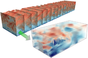
  $\boldsymbol {w}(\boldsymbol {x})$; cf. figure 1.

Figure 1. Normalized magnitudes of (a)  $\boldsymbol {\psi }$, (b)
  $\boldsymbol {u} = \operatorname {\boldsymbol {\nabla }\times }\boldsymbol {\psi }$ and (c)
  $\boldsymbol {w} = -\varDelta \boldsymbol {\psi }$. Observe the decrease of regularity, from left to right, with higher-order derivatives of the vector potential. The fields are computed using a discrete Fourier transform.
Remark 3.2 The spectral tensor (3.10) is sufficient to characterize the second-order statistics found in isotropic stationary and homogeneous turbulence. In turn, it is sufficient to characterize the kinetic energy and the Reynolds stresses and many of the other most important physical quantities in the flow (Pope Reference Pope2001, § 6.7.2). However, it is not sufficient to characterize higher-order effects, coherent structures, or intermittency, which are also well-known features of turbulent flows (see, e.g., She, Jackson & Orszag Reference She, Jackson and Orszag1990; Cao, Chen & Doolen Reference Cao, Chen and Doolen1999). Further work is required to incorporate non-Gaussian features.
4. Main results
In this section, we relate a large class of turbulent vector fields  $\boldsymbol {u}$ to the solution of a general family of FPDEs with stochastic forcing. In particular, we put forth a general inhomogeneous model, derive a corresponding model for shear flows and motivate a physically meaningful choice of boundary conditions.
4.1. A general class of inhomogeneous models
Equation (3.16) was derived from a very specific form of the energy spectrum function  $E(k)$. Under the same decomposition of the spectral tensor
  $\varPhi (\boldsymbol {x})$ given in (3.10), a much more general family of homogeneous and stationary random field models derive from the following ansatz on the energy spectrum function:
 \begin{equation} k^{{-}4}E(\boldsymbol{k}) = \mu^2 \det(\bar{\boldsymbol{\varTheta}})^{2/3\gamma}(1 +\boldsymbol{k}^\top\bar{\boldsymbol{\varTheta}}\boldsymbol{k})^{{-}2\alpha_1}(\boldsymbol{k}^\top\bar{\boldsymbol{\varTheta}}\boldsymbol{k})^{{-}2\alpha_2} . \end{equation}
Here,  $\bar {\boldsymbol {\varTheta }} \in \mathbb {R}^{3\times 3}$ is a fixed symmetric positive-definite matrix and
  $\alpha _2$,
  $\alpha _1$,
  $\gamma$ and
  $\mu$ are additional scalar parameters.
Equation (4.1) is a broad generalization of (3.11) which replaces  $E$ as function of
  $k = |\boldsymbol {k}|$ by
  $E$ as function of
  $\boldsymbol {k}$. This flexibility allows us, for example, to consider anisotropic effects. Indeed, just as
  $L$ played the role of a length scale in (3.11), here,
  $\bar {\boldsymbol {\varTheta }}$ plays the role of a metric in Fourier space. In addition, observe that if
  $\bar {\boldsymbol {\varTheta }}=L^2\boldsymbol{\mathsf{I}}$, where
  $\boldsymbol{\mathsf{I}}$ denotes the identity matrix,
  $4\alpha _2=4-p_0$,
  $4\alpha _1=5/3+p_0$,
  $\gamma = \alpha _1+\alpha _2$ and
  $\mu ^2=C \varepsilon ^{2/3}$, then (4.1) reproduces the following common one-parameter homogeneous energy spectrum model (see, e.g., Pope Reference Pope2001, p. 232):
 \begin{equation} E(k) = C \varepsilon^{2/3}k^{{-}5/3} \left(\frac{k L}{((k L)^2 + 1)^{1/2}} \right)^{5/3 + p_0}. \end{equation}
In this scenario,  $p_0=4$ corresponds exactly to the von Kármán spectrum (3.11) considered previously, i.e.
  $\alpha _1 = \gamma = {17}/{12}$ and
  $\alpha _2 = 0$.
As in (3.14), the vector potential  $\boldsymbol {\psi }(\boldsymbol {x}) = \int \operatorname {e}^{\operatorname {i}\boldsymbol {k}\boldsymbol {\cdot }\boldsymbol {x}} \,\mathrm {d} \boldsymbol {Y}(\boldsymbol {k})$ can also be written in terms of a Fourier–Stieltjes integral, weighted by
  $k^{-2} E^{1/2}(\boldsymbol {k})$. After rearranging factors, equation (4.1) characterizes the vector potential
  $\boldsymbol {\psi }$ as the solution of the following fractional stochastic PDE on
  $\mathbb {R}^3$:
 \begin{equation}
(I-\boldsymbol{\nabla}\boldsymbol{\cdot}(\bar{\boldsymbol{\varTheta}}\boldsymbol{\nabla}))^{\alpha_1}
(-\boldsymbol{\nabla}\boldsymbol{\cdot}(\bar{\boldsymbol{\varTheta}}\boldsymbol{\nabla}))^{\alpha_2}
\boldsymbol{\psi} = \mu\det(\bar{\boldsymbol{\varTheta}})^{\gamma/3}\boldsymbol{\xi}.
\end{equation}
\begin{equation}
(I-\boldsymbol{\nabla}\boldsymbol{\cdot}(\bar{\boldsymbol{\varTheta}}\boldsymbol{\nabla}))^{\alpha_1}
(-\boldsymbol{\nabla}\boldsymbol{\cdot}(\bar{\boldsymbol{\varTheta}}\boldsymbol{\nabla}))^{\alpha_2}
\boldsymbol{\psi} = \mu\det(\bar{\boldsymbol{\varTheta}})^{\gamma/3}\boldsymbol{\xi}.
\end{equation} Two immediate modifications of (4.3) are now in order. First, we may replace the constant matrix  $\bar{\boldsymbol{\varTheta}}$ by a spatially varying metric tensor
  $\boldsymbol {\varTheta }(\boldsymbol {x})$. This change immediately induces an inhomogeneous turbulence model. Second, we may consider substituting the white noise random variable
  $\boldsymbol {\xi }$ for a well-chosen coloured noise variable denoted
  ${\boldsymbol {\eta }}$. Together, these two generalizations lead to a family of random field models written
 \begin{equation} \left(I-\boldsymbol{\nabla}\boldsymbol{\cdot}(\boldsymbol{\varTheta}(\boldsymbol{x})\boldsymbol{\nabla})\right)^{\alpha_1}\left(-\boldsymbol{\nabla}\boldsymbol{\cdot}(\boldsymbol{\varTheta}(\boldsymbol{x})\boldsymbol{\nabla})\right)^{\alpha_2}\boldsymbol{\psi} = \mu\det(\boldsymbol{\varTheta}(\boldsymbol{x}))^{\gamma/3}{\boldsymbol{\eta}} . \end{equation}
 Physically, the metric tensor  $\boldsymbol {\varTheta }(\boldsymbol {x})$ introduces inhomogeneous and anisotropic diffusion; this corresponds to local changes of the turbulence length scales which may result from complicated dynamics of interacting eddies. Statistically, it incorporates the possibility for spatially varying correlation lengths and also may contain distortion.
In order to motivate one possible choice of the stochastic forcing term  ${\boldsymbol {\eta }}$, note that (4.2) can adequately characterize both the energy-containing and inertial subranges, however, it fails in the dissipative range; namely, where
  $k$ is large. In order to fit the dissipative range, one approach is to scale the energy spectrum with a decaying exponential function (see, e.g., Pope Reference Pope2001, p. 233):
 \begin{equation} E_{\beta}(k) = E(k)\operatorname{e}^{-\beta k}, \end{equation}
where  $\beta >0$ is a positive constant, usually close to the Kolmogorov length scale. In such scenarios, we suggest using the following definition for
  ${\boldsymbol {\eta }}$ in (4.4) (see Stein & Weiss Reference Stein and Weiss1971, Theorem 1.14):
 \begin{equation} \boldsymbol{\xi}_\beta(\boldsymbol{x}) = \int_{\mathbb{R}^3} \operatorname{e}^{\operatorname{i}\boldsymbol{k}\boldsymbol{\cdot}\boldsymbol{x}} \operatorname{e}^{-\beta k} \,\mathrm{d} \boldsymbol{W}(\boldsymbol{k}) \propto \boldsymbol{\xi}(\boldsymbol{x})\ast\frac{\beta}{(\beta^2 + |\boldsymbol{x}|^2)^{2}}, \end{equation}
which converges to (3.4) as  $\beta \to 0$. In the presence of shear, a different time-dependent modification is also natural to consider from the point of view of rapid distortion theory. That is the subject of the following subsection.
Remark 4.1 When  $\alpha _2$ and
  $\alpha _1$ are chosen to match the energy spectrum model (4.2), it is clear that
  $\alpha _2+\alpha _1 = 17/12$ is independent of
  $p_0$. Under this constraint,
  $\alpha _2$ mainly affect the behaviour of the power spectrum at the origin and, likewise, the large-scale structure of
  $\boldsymbol {u}$. In other words, the shape of the spectrum in the inertial subrange is unaffected by the precise choice of
  $\alpha _2$ and
  $\alpha _1 = 17/12-\alpha _2$; only the shape of the spectrum in the energy-containing range is affected (see figure 2). An illustration of some energy spectra possibilities is included in figure 2.

Figure 2. The energy spectrum  $E_{\beta }(k)/\mu ^2$ corresponding to (4.1) with
  $\bar {\boldsymbol {\varTheta }}=L^2\boldsymbol{\mathsf{I}}$. The sum
  $\alpha _2+\alpha _1$ is fixed to
  $17/12$, which guarantees the slope
  $k^{-5/3}$ in the inertial subrange. Different values of
  $\alpha _2$ control the energy-containing range. And the exponent
  $\beta /L=10^{-3}$ defines the exponential decay in the dissipative subrange.
4.2. A model for shear flows
Consider the velocity field  $\boldsymbol {U} = \langle \boldsymbol {U}\rangle + \boldsymbol {u}$ and define the average total derivative of the turbulent fluctuations
  $\boldsymbol {u} = (u_1,u_2,u_3)$ as follows:
 \begin{equation} \frac{\bar{D} u_i}{\bar{D} t} = \frac{\partial u_i}{\partial t} + \langle U_j\rangle\frac{\partial u_i}{\partial x_j}. \end{equation}
The rapid distortion equations (see, e.g. Townsend Reference Townsend1980; Maxey Reference Maxey1982; Hunt & Carruthers Reference Hunt and Carruthers1990) are a linearization of the Navier–Stokes equations in free space when the turbulence-to-mean-shear time scale ratio is arbitrarily large. They can be written
 \begin{equation} \frac{\bar{D} u_i}{\bar{D} t} ={-}u_i \frac{\partial \langle U_j\rangle}{\partial x_i} - \frac{1}{\rho}\frac{\partial p}{\partial x_i}, \quad \frac{1}{\rho} \varDelta p ={-}2\frac{\partial \langle U_i\rangle}{\partial x_j}\frac{\partial u_j}{\partial x_i}. \end{equation}
 Under a uniform shear mean velocity gradient,  $\langle U_i(\boldsymbol {x})\rangle = x_j\partial \langle U_i\rangle / \partial x_j$, where
  $\partial \langle U_i\rangle / \partial x_j$ is a constant tensor, a well-known form of these equations can be written out in Fourier space. In this case, the rate of change of each frequency
  $\boldsymbol {k}(t) = (k_1(t),k_2(t),k_3(t))$ is defined
  ${\mathrm {d} k_i}/{\mathrm {d} t} = -k_j{\partial \langle U_j\rangle }/{\partial x_i}$. We then have the following Fourier representation of the average total derivative of
  $\boldsymbol {u}$:
 \begin{equation} \frac{\bar{D} u_i}{\bar{D} t} = \int_{\mathbb{R}^3} \operatorname{e}^{\operatorname{i}\boldsymbol{k}\boldsymbol{\cdot}\boldsymbol{x}}\left( \left(\frac{\partial }{\partial t} + \frac{\mathrm{d} k_j}{\mathrm{d} t}\frac{\partial }{\partial k_j}\right) \,\mathrm{d} Z_i(\boldsymbol{k},t) \right) = \int_{\mathbb{R}^3} \operatorname{e}^{\operatorname{i}\boldsymbol{k}\boldsymbol{\cdot}\boldsymbol{x}}\left(\frac{\bar{D} \,\mathrm{d} Z_i(\boldsymbol{k},t)}{\bar{D} t}\right) . \end{equation}
With this expression, the Fourier representation of (4.8a,b) can be written
 \begin{equation} \frac{\bar{D} \,\mathrm{d} Z_j(\boldsymbol{k},t)}{\bar{D} t} = \frac{\partial U_\ell}{\partial x_k} \left( 2 \frac{k_j k_\ell}{k^2} - \delta_{j\ell} \right) \,\mathrm{d} Z_k(\boldsymbol{k},t). \end{equation}
 Exact solutions to (4.10) are well-known (see, e.g., Townsend Reference Townsend1980; Mann Reference Mann1994), given the initial conditions  $\boldsymbol {k}_0 = (k_{10},k_{20},k_{30})$ and
  $\mathrm {d} \boldsymbol {Z}(\boldsymbol {k}_0,0)$. In the scenario
 \begin{equation} \langle \boldsymbol{U}(\boldsymbol{x})\rangle = (U_0 + S x_3) \boldsymbol{e}_1 , \end{equation}
the solution can be written in terms of the evolving Fourier modes  $\boldsymbol {k}(t)$ and non-dimensional time
  $\tau = S t$, as follows:
 \begin{equation} \mathrm{d} \boldsymbol{Z}(\boldsymbol{k},t) = \boldsymbol{\mathsf{D}}_\tau(\boldsymbol{k}) \mathrm{d} \boldsymbol{Z}(\boldsymbol{k}_0,0) , \end{equation}
where
 \begin{equation} \boldsymbol{\mathsf{D}}_\tau(\boldsymbol{k}) = \begin{bmatrix} 1 & 0 & \zeta_1\\ 0 & 1 & \zeta_2\\ 0 & 0 & \zeta_3 \end{bmatrix} , \quad \boldsymbol{k}_0 = \boldsymbol{\mathsf{T}}_\tau \boldsymbol{k} , \quad \boldsymbol{\mathsf{T}}_\tau = \begin{bmatrix} 1 & 0 & 0 \\ 0 & 1 & 0 \\ \tau & 0 & 1 \end{bmatrix} . \end{equation}
In the expression for  $\boldsymbol{\mathsf{D}}_\tau (\boldsymbol {k})$, the non-dimensional coefficients
  $\zeta _i = \zeta _i(\boldsymbol {k},\tau )$,
  $i=1,2,3$, are defined
 \begin{equation} \zeta_1 = C_1 - C_2 k_2/k_1, \quad \zeta_2 = C_1 k_2/k_1 + C_2, \quad \zeta_3 = k_0^2/k^2, \end{equation}
where  $k_0 = |\boldsymbol {k}_0|$ and
 \begin{align} C_1 = \frac{\tau k_1^2(k_0^2 -2k_{30}^2 + \tau k_1 k_{30})}{k^2(k_1^2+k_2^2)}, \quad C_2 = \frac{k_2 k_0^2}{(k_1^2+k_2^2)^{3/2}} \arctan\left( \frac{\tau k_1(k_1^2 + k_2^2)^{1/2}}{k_0^2 - \tau k_{30}k_1} \right) . \end{align}
One may observe that
 \begin{equation} \begin{bmatrix} 1 & 0 & \zeta_1\\ 0 & 1 & \zeta_2\\ 0 & 0 & \zeta_3 \end{bmatrix} \begin{bmatrix} 0 & -k_{30} & k_2\\ k_{30} & 0 & -k_1\\ -k_2 & k_1 & 0 \end{bmatrix} = \begin{bmatrix} 0 & -k_{3} & k_2\\ k_3 & 0 & -k_1\\ -k_2 & k_1 & 0 \end{bmatrix} \begin{bmatrix} \zeta_3 & 0 & 0\\ 0 & \zeta_3 & 0\\ -\zeta_1 & -\zeta_2 & 1 \end{bmatrix} , \end{equation}
or, equivalently,  $\boldsymbol{\mathsf{D}}_\tau (\boldsymbol {k}) k_0^{-2}\boldsymbol{\mathsf{Q}}(\boldsymbol {k}_0) = k^{-2}\boldsymbol{\mathsf{Q}}(\boldsymbol {k}) \boldsymbol{\mathsf{D}}_\tau ^{-\top }(\boldsymbol {k})$. Moreover,
  $\mathrm {d}\boldsymbol {W}(\boldsymbol {k}_0) = \mathrm {d}\boldsymbol {W}(\boldsymbol {k})$, owing to translational invariance. Therefore, taking
  $\mathrm {d} \boldsymbol {Z}(\boldsymbol {k}_0,0) = \boldsymbol{\mathsf{Q}}(\boldsymbol {k}_0) (({1}/{\sqrt {4{\rm \pi} }k_0^2}) E^{1/2} (\boldsymbol {k}_0) \,\mathrm {d}\boldsymbol {W}(\boldsymbol {k}_0)) ,$ it holds that
 \begin{equation} \mathrm{d} \boldsymbol{Z}(\boldsymbol{k},t) = \boldsymbol{\mathsf{Q}}(\boldsymbol{k}) \left(\frac{1}{\sqrt{4{\rm \pi}}k^2} E^{1/2}(\boldsymbol{\mathsf{T}}_\tau\boldsymbol{k})\, \boldsymbol{\mathsf{D}}_\tau^{-\top}(\boldsymbol{k})\,\mathrm{d}\boldsymbol{W}(\boldsymbol{k})\right) . \end{equation}
Finally, invoking the general expression for  $E(\boldsymbol {k})$ written in (4.1), one arrives at the rapid distortion equation FPDE
 \begin{equation} \left(I-\boldsymbol{\nabla}\boldsymbol{\cdot}(\bar{\boldsymbol{\varTheta}}_\tau\boldsymbol{\nabla})\right)^{\alpha_1}\left(-\boldsymbol{\nabla}\boldsymbol{\cdot}(\bar{\boldsymbol{\varTheta}}_\tau\boldsymbol{\nabla})\right)^{\alpha_2}\boldsymbol{\psi} = \mu\det(\bar{\boldsymbol{\varTheta}}_\tau)^{\gamma/3}{\boldsymbol{\eta}}_\tau \end{equation}
where  $\bar {\boldsymbol {\varTheta }}_\tau = \boldsymbol{\mathsf{T}}_\tau ^\top \bar {\boldsymbol {\varTheta }} \boldsymbol{\mathsf{T}}_\tau$ and
  ${\boldsymbol {\eta }}_\tau (\boldsymbol {x}) = \int _{\mathbb {R}^3} \operatorname {e}^{\operatorname {i}\boldsymbol {k}\boldsymbol {\cdot }\boldsymbol {x}} (\boldsymbol{\mathsf{D}}_\tau ^{-\top }(\boldsymbol {k})\,\mathrm {d}\boldsymbol {W}(\boldsymbol {k}) )$. Note that
  $\det (\bar {\boldsymbol {\varTheta }}_\tau ) = \det (\bar {\boldsymbol {\varTheta }})$.
Remark 4.2 For each fixed  $t$, equation (4.18) is clearly a particular case of (4.4). The generalization of this model to an inhomogeneous instationary FPDE is discussed in § 5.2.
Remark 4.3 An important extension of the rapid distortion model above involves replacing the constant  $\tau$ by a wavenumber-dependent ‘eddy lifetime’
  $\tau (k)$ (see, e.g., Mann Reference Mann1994). Such models are considered more realistic because, at some point, the shear from the mean velocity gradient will cause the eddies to stretch and eventually they will breakup within a size-dependent timescale. In this case, the generalization of
  ${\boldsymbol {\eta }}_\tau$ above is straightforward. Meanwhile, at least when
  $\bar {\boldsymbol {\varTheta }} = L^2 \boldsymbol{\mathsf{I}}$, one may consider replacing the operator
  $\bar {\boldsymbol {\varTheta }}_\tau$ in (4.18) by
 \begin{equation} L^2\,
\mathcal{F}^{-1} \begin{bmatrix} 1+\tau(k)^2 & 0 & \tau(k) \\
0 & 1 & 0 \\ \tau(k) & 0 & 1 \end{bmatrix}
\mathcal{F}.
\end{equation}
\begin{equation} L^2\,
\mathcal{F}^{-1} \begin{bmatrix} 1+\tau(k)^2 & 0 & \tau(k) \\
0 & 1 & 0 \\ \tau(k) & 0 & 1 \end{bmatrix}
\mathcal{F}.
\end{equation}To solve such an equation numerically, one does not need to construct the closed form of the linear operator, but may instead choose to use a matrix-free Krylov method (Saad Reference Saad2003).
4.3. Boundary conditions
There are a number of different, equivalent, definitions of fractional operators on  $\mathbb {R}^3$. However, moving from the free-space equation (4.4) to a boundary value problem relies on heuristics and can be done in a wide variety of ways; each of which may also differ by the specific definition of the fractional operator being used (Lischke et al. Reference Lischke2020). As stated previously, in this work, we choose to only deal with the spectral definition. In this setting, boundary conditions are applied to the corresponding integer-order operator and then incorporated implicitly by modifying the spectrum; cf. (3.6) and (3.7).
Assume that (4.4) is posed on a three-dimensional simply connected domain  $\varOmega \subsetneq \mathbb {R}^3$ with boundary
  $\varGamma = \partial \varOmega$. We begin with the following heuristically chosen impermeability condition for the velocity field:
 \begin{equation} \boldsymbol{u} = \operatorname{\boldsymbol{\nabla}\times} \boldsymbol{\psi} \quad \text{in } \varOmega , \quad \boldsymbol{u}\boldsymbol{\cdot}\boldsymbol{n} = 0 \quad \text{on } \varGamma . \end{equation}
Although more relaxed boundary conditions are also possible, we choose to enforce (4.20) via a no-slip condition on the vector potential  $\boldsymbol {\psi }$; specifically,
 \begin{equation} \boldsymbol{\psi} - (\boldsymbol{\psi}\boldsymbol{\cdot}\boldsymbol{n})\boldsymbol{n} = \boldsymbol{0} \quad \text{on } \varGamma . \end{equation}
It turns out that (4.21) is not enough to uniquely define  $\boldsymbol {\psi }$ on
  $\varOmega$. In fact, the remaining boundary condition must restrict
  $\boldsymbol {\psi }$ normal to
  $\varGamma$.
We are somewhat free to select what the remaining boundary condition will be. Both the Dirichlet-type boundary condition  $\boldsymbol {\psi }\boldsymbol {\cdot }\boldsymbol {n} = 0$ and the Neumann-type boundary condition
  $(\boldsymbol {\varTheta }(\boldsymbol {x})\boldsymbol {\nabla }\boldsymbol {\psi })\boldsymbol {n}\boldsymbol {\cdot } \boldsymbol {n} = 0$ are possible candidates which would close the equations. Another option is to enforce a weighted average of those two boundary conditions. To be more specific, we may also consider the generalized (homogeneous) Robin boundary condition
 \begin{equation} \kappa\boldsymbol{\psi}\boldsymbol{\cdot}\boldsymbol{n} + (\boldsymbol{\varTheta}(\boldsymbol{x})\boldsymbol{\nabla}\boldsymbol{\psi})\boldsymbol{n}\boldsymbol{\cdot} \boldsymbol{n} = 0 \quad \text{on } \varGamma , \end{equation}
where the new model parameter  $\kappa \geq 0$ could be inferred from available data.
In this work, we choose to close the equations with (4.22) because it is flexible enough to fit a wide variety of data and simple to implement alongside (4.21). We note that  $\kappa$ affects the horizontal velocity near the surface because of its control over the normal component of
  $\boldsymbol {\psi }$. Thus, in the proposed model,
  $\kappa$ may be a parameter which distinguishes between different types of surfaces. We also note that, in the limit
  $\kappa \to \infty$, we recover the boundary condition
  $\boldsymbol {\psi }\boldsymbol {\cdot }\boldsymbol {n} = 0$. Together with (4.21), it implies the complete Dirichlet boundary condition,
  $\boldsymbol {\psi } = \boldsymbol {0}$ on
  $\varGamma$. Hereon, we use the notation
  $\kappa =\infty$ to indicate this special limiting scenario.
Note that (4.4) can be written  $\mathcal {L}\boldsymbol {\psi } = \boldsymbol {b}$, where
 \begin{align} \mathcal{L} := \left(I-\boldsymbol{\nabla}\boldsymbol{\cdot}(\boldsymbol{\varTheta}(\boldsymbol{x})\boldsymbol{\nabla})\right)^{\alpha_1}\left(-\boldsymbol{\nabla}\boldsymbol{\cdot}(\boldsymbol{\varTheta}(\boldsymbol{x})\boldsymbol{\nabla})\right)^{\alpha_2} \quad\text{and}\quad \boldsymbol{b} := \mu\det(\boldsymbol{\varTheta}(\boldsymbol{x}))^{\gamma/3}{\boldsymbol{\eta}} . \end{align}
In order to define the domain  $\mathcal {D}(\mathcal {L})$ of the multi-fractional operator
  $\mathcal {L}\colon \mathcal {D}(\mathcal {L}) \subseteq [L^2(\varOmega )]^3 \to [L^2(\varOmega )]^3$, we start by letting
  $A := (I\,{-}\,\boldsymbol {\nabla }\boldsymbol {\cdot }(\boldsymbol {\varTheta }(\boldsymbol {x})\boldsymbol {\nabla })) \colon \mathcal {D}(A) \,{\subseteq}\, [L^2(\varOmega )]^3 \to [L^2(\varOmega )]^3$. For notational convenience, we assume that
  $A$ has a discrete spectrum.
In the spectral definition of  $A^{\alpha _1}$, the domain
  $\mathcal {D}(A)$ characterizes the boundary conditions on
  $\varGamma$. In this work, assuming that
  $\det (\boldsymbol {\varTheta }(\boldsymbol {x}))$ is uniformly bounded from above and below by positive constants, we define
 \begin{equation}
\mathcal{D}(A) = \{ \boldsymbol{\psi} \in
[H^2(\varOmega)]^3 \colon \eqref{eqn48}\hbox{ and }\eqref{eqn48}\hbox{ hold in the sense of traces} \} .
\end{equation}
\begin{equation}
\mathcal{D}(A) = \{ \boldsymbol{\psi} \in
[H^2(\varOmega)]^3 \colon \eqref{eqn48}\hbox{ and }\eqref{eqn48}\hbox{ hold in the sense of traces} \} .
\end{equation}
For this operator domain, there exists an orthonormal basis of eigenvectors  $\{\boldsymbol {a}_j\}_{j=1}^\infty \subseteq \mathcal {D}(A)$, with corresponding eigenvalues
  $\{a_j\}_{j=1}^\infty$ in non-increasing order (cf. Bolin, Kirchner & Kovács Reference Bolin, Kirchner and Kovács2020). Then, following (3.7), the fractional differential operator
  $A^{\alpha _1} \colon \mathcal {D}(A^{\alpha _1}) \subseteq [L^2(\varOmega )]^3 \to [L^2(\varOmega )]^3$ is defined
 \begin{equation} A^{\alpha_1}\boldsymbol{\psi} = \sum_{j=1}^\infty a_j^{\alpha_1} (\boldsymbol{\psi},\boldsymbol{a}_j)_\varOmega\, \boldsymbol{a}_j \end{equation}
and  $\mathcal {D}(A^{\alpha _1}) = \{ \boldsymbol {\psi } \in [L^2(\varOmega )]^3\, \colon \sum _{j=1}^\infty a_j^{2\alpha _1} (\boldsymbol {\psi },\boldsymbol {a}_j)_\varOmega ^2 < \infty \}$.
Now consider  $A-I \colon \mathcal {D}(A) \to [L^2(\varOmega )]^3$ and note that
  $\mathcal {L} = A^{\alpha _1} (A-I)^{\alpha _2}$. In this case,
  $A^{\alpha _1}$ and
  $(A-I)^{\alpha _2}$ commute because they share the same eigenmodes:
 \begin{equation} A^{\alpha_1} (A-I)^{\alpha_2} \boldsymbol{\psi} = \sum_{j=1}^\infty a_j^{\alpha_1} (a_j-1)^{\alpha_2} (\boldsymbol{\psi},\boldsymbol{a}_j)_\varOmega\, \boldsymbol{a}_j = (A-I)^{\alpha_2} A^{\alpha_1}\boldsymbol{\psi} . \end{equation}
Accordingly, we define the domain of the operator  $\mathcal {L}$ as follows:
 \begin{equation} \mathcal{D}(\mathcal{L}) = \left\{ \boldsymbol{\psi} \in [L^2(\varOmega)]^3\, \colon \sum_{j=1}^\infty a_j^{2\alpha_1}(a_j-1)^{2\alpha_2} (\boldsymbol{\psi},\boldsymbol{a}_j)_\varOmega^2 < \infty\right\} . \end{equation}
 We may now write the boundary value problem given by (4.4), (4.21) and (4.22) as the abstract operator equation  $\mathcal {L}\boldsymbol {\psi } = \boldsymbol {b}$, with
  $\mathcal {D}(\mathcal {L})$ defined in (4.27). Nevertheless, we will still usually refer to this problem in the ‘strong form’
 \begin{equation} \left. \begin{array}{cl} \left(I-\boldsymbol{\nabla}\boldsymbol{\cdot}(\boldsymbol{\varTheta}(\boldsymbol{x})\boldsymbol{\nabla})\right)^{\alpha_1}\left(-\boldsymbol{\nabla}\boldsymbol{\cdot}(\boldsymbol{\varTheta}(\boldsymbol{x})\boldsymbol{\nabla})\right)^{\alpha_2}\boldsymbol{\psi} = \mu\det(\boldsymbol{\varTheta}(\boldsymbol{x}))^{\gamma/3}{\boldsymbol{\eta}}, & \text{in}\ \varOmega,\\ \boldsymbol{\psi} - (\boldsymbol{\psi}\boldsymbol{\cdot}\boldsymbol{n})\boldsymbol{n} = 0, & \text{on}\ \varGamma,\\ \kappa\boldsymbol{\psi}\boldsymbol{\cdot}\boldsymbol{n} + (\boldsymbol{\varTheta}(\boldsymbol{x})\boldsymbol{\nabla}\boldsymbol{\psi})\boldsymbol{n}\boldsymbol{\cdot}\boldsymbol{n} = 0, & \text{on}\ \varGamma, \end{array} \right\} \end{equation}
because it is much more physically illustrative.
5. Physical applications
In this section, we document three applications of (4.28) and some theoretical results. The first two applications describe turbulent conditions which may be modelled using the general FPDE model (4.28). In the final subsection, we highlight an important wind engineering application. Here, the model is used to generate a turbulent inlet profile for a numerical wind tunnel simulation of the atmospheric boundary layer.
5.1. Shear-free boundary layers
There are many different examples of turbulence confined by a solid boundary, without any significant mean shear (Hunt Reference Hunt1984). In such flows, the rate of turbulent kinetic energy dissipation  $\epsilon$ can be assumed to be approximately constant with height. This setting has been studied in detail by various authors (see, e.g., Hunt Reference Hunt1984; Hunt et al. Reference Hunt, Moin, Lee, Moser, Spalart, Mansour, Kaimal and Gaynor1989; Perot & Moin Reference Perot and Moin1995a,Reference Perot and Moinb; Aronson, Johansson & Löfdahl Reference Aronson, Johansson and Löfdahl1997 and references therein) and so forms a solid proving ground to validate (4.28).
5.1.1. A von Kármán-type model
We begin with the inhomogeneous turbulence model (4.28), with fractional coefficients corresponding to the von Kármán energy spectrum (3.11), on the open half space domain  $\mathbb {R}_+^3 = \{ (x,y,z) \in \mathbb {R}^3 \colon z >0 \}$. Based on the supposed absence of shear, we also consider the following simple diagonal form for the diffusion tensor, in Cartesian coordinates:
 \begin{equation} \boldsymbol{\varTheta}(z) = \begin{bmatrix} L_{1}(z)^2 & 0 & 0 \\ 0 & L_{2}(z)^2 & 0 \\ 0 & 0 & L_{3}(z)^2 \end{bmatrix} . \end{equation}
Defining  $L(z) = \sqrt [3]{L_1(z)L_2(z)L_3(z)}$, the appropriate form of (4.28) can be written as follows:
 \begin{equation} \left. \begin{array}{cl} \left(I-\operatorname{\boldsymbol{\nabla}\hspace{1.25pt}\boldsymbol{\cdot}}(\boldsymbol{\varTheta}(z)\boldsymbol{\nabla})\right)^{17/12} \boldsymbol{\psi}= \mu L(z)^{17/6} \boldsymbol{\xi}, & \text{in}\ \mathbb{R}_+^3, \\ \kappa\psi_3 + L_{3}(z)^2 \dfrac{\partial\psi_3}{\partial z} = \psi_1 = \psi_2 = 0, & \text{at}\ z=0 . \end{array} \right\} \end{equation}
 Both the Robin coefficient  $\kappa$ and an explicit parametric expression for each
  $L_i(z)$ give rise to a model design parameter vector, say
  ${\boldsymbol {\theta }}$. This vector
  ${\boldsymbol {\theta }}$ may then be subject to calibration with respect to experimental data, e.g. using the technique described in § 6.2. This process of model calibration is important because wall roughness, Reynolds number and the nature of the turbulence may affect the near-wall statistics (Pope Reference Pope2001) and may be incorporated through proper parameter selection. For instance, let us consider the following exponential expansion
 \begin{equation} L_i(z) = L_\infty \cdot\left(1 + \sum_{k=1}^K c_{i,k}\operatorname{e}^{{-}d_{i,k} ({z}/{L_\infty})} \right) , \end{equation}
with each  $d_{i,k}\ge 0$,
  $c_{1,k} = c_{2,k}$ and
  $d_{1,k} = d_{2,k}$. Taking only two terms in each expansion above (
 $K=2$), we arrive through calibration at a statistical model which closely matches the experimental data found in Thomas & Hancock (Reference Thomas and Hancock1977). Note that with such a model,
  $L_1(z) = L_2(z)$ and each
  $L_i(z)$ exponentially converges to the homogeneous length scale
  $L_\infty$, as
  $z\to \infty$, as illustrated in figure 3.

Figure 3. Optimal diffusion coefficients  $L_i(z)$ and Robin constant
  $\kappa$ determined by fitting the Reynolds stress data in figure 4. Note that
  $L_1(z) = L_2(z)$.
The prescribed boundary conditions will affect the physical length scales of the random velocity field  $\boldsymbol {u} = \boldsymbol {\nabla } \times \boldsymbol {\psi }$. Therefore, the diffusion coefficients
  $L_i(z)$ do not necessarily correspond to the physical length scales. For this reason, we follow Lee & Hunt (Reference Lee and Hunt1991) and define the (physical) so-called integral length scales
 \begin{equation}
\ell_{ij}^{(x_m)}(z) = \frac{\displaystyle\int_{\mathbb{R}}\langle
u_i(\boldsymbol{x} + r\boldsymbol{e}_m)
u_j(\boldsymbol{x})\rangle\,\mathrm{d} r}{\langle
u_i(\boldsymbol{x}) u_j(\boldsymbol{x})\rangle} =
\frac{\displaystyle\int_{\mathbb{R}} R_{ij}(r\boldsymbol{e}_m,z)
\,\mathrm{d} r}{R_{ij}(\boldsymbol{0},z)} .
\end{equation}
\begin{equation}
\ell_{ij}^{(x_m)}(z) = \frac{\displaystyle\int_{\mathbb{R}}\langle
u_i(\boldsymbol{x} + r\boldsymbol{e}_m)
u_j(\boldsymbol{x})\rangle\,\mathrm{d} r}{\langle
u_i(\boldsymbol{x}) u_j(\boldsymbol{x})\rangle} =
\frac{\displaystyle\int_{\mathbb{R}} R_{ij}(r\boldsymbol{e}_m,z)
\,\mathrm{d} r}{R_{ij}(\boldsymbol{0},z)} .
\end{equation}
In these expressions, we have accounted for the fact that all solutions of (5.2) are temporary stationary and statistically homogeneous in the  $x$- and
  $y$-directions, i.e.
  $R(\boldsymbol {r},\boldsymbol {x},t) = R(\boldsymbol {r},z)$.
In § 6, we explain how to solve this problem numerically and to calibrate its solutions to Reynolds stress data. The difference between the Reynolds stress profiles in the calibrated model and the corresponding experimental data is depicted in figure 4, alongside the resulting integral length scales  $\ell _{ij}^{(x_m)}(z)$. Because this model has many free parameters which can be calibrated to experimental data, it is much more flexible than the classical theory proposed by Hunt (Reference Hunt1973, Reference Hunt1984) and Hunt & Graham (Reference Hunt and Graham1978). Indeed, a comparison between the two theories, which highlights this flexibility, is given in the next subsection. Note that the exact definitions of the optimized model parameters used in the results above are stated explicitly in the table in figure 3.

Figure 4. Reynolds stress data from Thomas & Hancock (Reference Thomas and Hancock1977) compared with Reynolds stresses from (a) the calibrated SFBL turbulence model (5.2) and (b) corresponding integral length scales. Observe that the model is able to closely fit the experimental data.
5.1.2. Comparison with the classical theory
It is important to consider the special case of (5.2) where each  $L_i(z)$ is constant in
  $z$. In Hunt's idealized shear-free boundary layer (SFBL) theory (Hunt & Graham Reference Hunt and Graham1978; Hunt Reference Hunt1984), derived from the energy spectrum ansatz (3.11) and briefly summarized in § 2, one can show that
 \begin{equation} \frac{\langle u^2 \rangle}{\langle u^2_\infty \rangle} = \frac{\langle v^2 \rangle}{\langle v^2_\infty \rangle} \to 1.5 \quad\text{and} \quad \frac{\langle w^2 \rangle}{\langle w^2_\infty \rangle} = O\left(\left(\frac{z}{L_\infty}\right)^{2/3}\right) \quad\text{as} \ \frac{z}{L_\infty} \to 0, \end{equation}
where  $\langle u^2_\infty \rangle = \langle v^2_\infty \rangle = \langle w^2_\infty \rangle$ denotes the far-field limit
  $z\to \infty$ of the non-zero Reynolds stresses. The limit
  $\langle u^2 \rangle /\langle u^2_\infty \rangle \to 1.5$ is not always achieved in experiments (cf. figure 4), however, the limiting behaviour
  $\langle w^2 \rangle /\langle w^2_\infty \rangle = O((z/L_\infty )^{2/3})$ is well-established in the literature (Priestley Reference Priestley1959; Kaimal et al. Reference Kaimal, Wyngaard, Haugen, Coté, Izumi, Caughey and Readings1976).
The corresponding scenario in our class of models is exactly (5.2) with each  $L_i = L_\infty$. In this setting, the non-zero Reynolds stresses,
  $\langle u^2 \rangle = \langle v^2 \rangle$ and
  $\langle w^2 \rangle$, can be derived analytically, at least for certain values of
  $\kappa \geq 0$. These exact analytical solutions are summarized in Lemmas 5.1–5.3, the proofs of which can be found in Appendix A. Exact analytical solutions for the integral length scales
  $\ell _{ij}^{(x_m)}(z)$ can also be derived by a similar technique, but we do not include their derivation in this work for the sake of brevity. Plots of the analytical Reynolds stresses and integral length scales are depicted in figure 5.
Lemma 5.1 Given  $\boldsymbol {u} = (u,v,w) = \boldsymbol {\nabla }\times \boldsymbol {\psi }$, where
  $\boldsymbol {\psi }$ is any solution of (5.2) with constant
  $L_1 = L_2 = L_\infty$, it holds that
 \begin{equation} \frac{\langle w^2 \rangle}{\langle w^2_\infty \rangle} = 1 - \mathcal{M}_{1/3}\left(\frac{2z}{L_\infty}\right) , \end{equation}
where  $\mathcal {M}_{\nu }(x)$ is the Matérn kernel (Matérn Reference Matérn1986; Stein Reference Stein1999; Khristenko et al. Reference Khristenko, Scarabosio, Swierczynski, Ullmann and Wohlmuth2019) given by
 \begin{equation} \mathcal{M}_{\nu}(x) = \frac{x^\nu\mathrm{K}_{\nu}(x)}{2^{\nu-1}\varGamma(\nu)}, \quad \nu \geq 0, \end{equation}
and  $\mathrm {K}_{\nu }(x)$ denotes the modified Bessel function of the second kind (Abramowitz & Stegun Reference Abramowitz and Stegun1948; Bateman Reference Bateman1953; Watson Reference Watson1995). Moreover, near the boundary the following asymptotic holds:
 \begin{equation} \frac{\langle w^2 \rangle}{\langle w^2_\infty \rangle} \sim \frac{\varGamma(2/3)}{\varGamma(4/3)} \left(\frac{z}{L_\infty}\right)^{2/3} \quad\text{as} \ \frac{z}{L_\infty} \to 0 . \end{equation}
Lemma 5.2 Given  $\boldsymbol {u} = (u,v,w) = \boldsymbol {\nabla }\times \boldsymbol {\psi }$, where
  $\boldsymbol {\psi }$ is the solution of (5.2) with constant
  $\boldsymbol {\varTheta } = L_\infty ^2\boldsymbol{\mathsf{I}}$ and
  $\kappa =0$, it holds that
 \begin{equation} \frac{\langle u^2 \rangle}{\langle u^2_\infty \rangle} = \frac{\langle v^2 \rangle}{\langle v^2_\infty \rangle} = 1 + (\nu+1)\mathcal{M}_{\nu}\left(\frac{2z}{L_\infty}\right) - \nu\mathcal{M}_{\nu+1}\left(\frac{2z}{L_\infty}\right) . \end{equation}
Hence, near the boundary,
 \begin{equation} \frac{\langle u^2 \rangle}{\langle u^2_\infty \rangle} = \frac{\langle v^2 \rangle}{\langle v^2_\infty \rangle} \to 2 \quad \textrm{as}\ \frac{z}{L_\infty} \to 0. \end{equation}
Lemma 5.3 Given  $\boldsymbol {u} = (u,v,w) = \boldsymbol {\nabla }\times \boldsymbol {\psi }$, where
  $\boldsymbol {\psi }$ is any solution of (5.2) with constant
  $\boldsymbol {\varTheta } = L_\infty ^2\boldsymbol{\mathsf{I}}$ and
  $\kappa =\infty$, it holds that
 \begin{equation} \frac{\langle u^2 \rangle}{\langle u^2_\infty \rangle} = \frac{\langle v^2 \rangle}{\langle v^2_\infty \rangle} = 1 + \nu\mathcal{M}_{\nu}\left(\frac{2z}{L_\infty}\right) - \nu\mathcal{M}_{\nu+1}\left(\frac{2z}{L_\infty}\right). \end{equation}
Hence, near the boundary,
 \begin{equation} \frac{\langle u^2 \rangle}{\langle u^2_\infty \rangle} = \frac{\langle v^2 \rangle}{\langle v^2_\infty \rangle} \to 1 \quad \textrm{as}\ \frac{z}{L_\infty} \to 0. \end{equation}
Remark 5.4 The Robin boundary condition  $\kappa \psi _3 + L_\infty ^2 ({\partial \psi _3}/{\partial z}) = 0$ has no effect on
  $\langle w^2 \rangle$. Therefore, the asymptotic expansion of the well-known (Priestley Reference Priestley1959; Kaimal et al. Reference Kaimal, Wyngaard, Haugen, Coté, Izumi, Caughey and Readings1976; Hunt Reference Hunt1984; Hunt et al. Reference Hunt, Moin, Lee, Moser, Spalart, Mansour, Kaimal and Gaynor1989) asymptotic behaviour
  $\langle w^2 \rangle /\langle w^2_\infty \rangle = O((z/L_\infty )^{2/3})$ as
  $z/L_\infty \to 0$ always holds when
  $L_1 = L_2 = L_\infty$.
Remark 5.5 The limit  $\langle u^2 \rangle /\langle u^2_\infty \rangle \to 1.5$ from Hunt's theory lies exactly in between the range of analogous limits,
  $\langle u^2 \rangle /\langle u^2_\infty \rangle \to 1$ and
  $\langle u^2 \rangle /\langle u^2_\infty \rangle \to 2$, coming from the exact solutions of (5.2) when
  $\kappa = \infty$ and
  $\kappa = 0$, respectively. Numerical experiments show that
  $\langle u^2 \rangle /\langle u^2_\infty \rangle = \langle v^2 \rangle /\langle v^2_\infty \rangle$ always limits to a value in the interval
  $(1,2)$ when
  $\kappa \in (0,\infty )$ and
  $\boldsymbol {\varTheta } = L_\infty ^2\boldsymbol{\mathsf{I}}$.
5.1.3. A more general energy spectrum
In order to illustrate the dependence of (4.28) on the parameter  $\alpha _2 = 17/12 -\alpha _1$, we may consider an alternative form of (5.2) which corresponds to the energy spectrum (4.2) with
  $p_0 = 2$. Here, for additional complexity, we also consider the load
  ${\boldsymbol {\eta }} = \boldsymbol {\xi }_\beta$ with
  $\beta /L_\infty =10^{-2}$:
 \begin{equation} \left. \begin{array}{cl} \left(I-\operatorname{\boldsymbol{\nabla}\hspace{1.25pt}\boldsymbol{\cdot}}(\boldsymbol{\varTheta}(z)\boldsymbol{\nabla})\right)^{11/12} \left(-\operatorname{\boldsymbol{\nabla}\hspace{1.25pt}\boldsymbol{\cdot}}(\boldsymbol{\varTheta}(z)\boldsymbol{\nabla})\right)^{1/2} \boldsymbol{\psi} = \mu L(z)^{17/6} \boldsymbol{\xi}_\beta, & \text{in}\ \mathbb{R}_+^3,\\ \kappa\psi_3 + L_3(z)^2 \dfrac{\partial\psi_3}{\partial z} = \psi_1 = \psi_2 = 0 , & \text{at}\ z=0 . \end{array} \right\} \end{equation}
 We do not analyze these equations in detail here, however, we present a single realization of their solution figure 6 for visual comparison. Observe that the velocity field coming from (5.13) is visibly smoother than its counterpart coming from (5.2). This is due to the high regularity load  $\boldsymbol {\xi }_\beta$.

Figure 6. Normalized magnitudes of  $\boldsymbol {u} = \operatorname {\boldsymbol {\nabla }\times }\boldsymbol {\psi }$ from (a) (5.2), (b) (5.13) with
  $\beta /L_\infty = 10^{-2}$ and (c) (5.15) with
  $\tau = 1.0$. The additional model parameters are specified in figure 3. Observe that the central field is visibly smoother than its counterpart on the left owing to the high regularity load
  $\boldsymbol {\xi }_\beta$. The field on the right, issued from the same noise, presents distortion.
5.2. Uniform shear boundary layers
Classically, rapid distortion theory is used to describe the short time evolution of isotropic turbulence. As pointed out in, e.g., Lee & Hunt (Reference Lee and Hunt1991), it is also possible to extend its use to some examples of inhomogeneous turbulence. In this example, we follow Lee & Hunt (Reference Lee and Hunt1991) in considering a uniform shear boundary layer (USBL) model where the only effect of the wall is to block velocity fluctuations in the normal direction. Our derivation begins from the assumption  $\langle \boldsymbol {U}(\boldsymbol {x})\rangle = (U_0 + S x_3) \boldsymbol {e}_1$ taken in § 4.2, but we also allow for a
  $z$-dependent inhomogeneous diffusion tensor,
 \begin{equation} \boldsymbol{\varTheta}_\tau(z) = \begin{bmatrix} L_1(z)^2+\tau^2 L_3(z)^2 & 0 & \tau L_3(z)^2\\ 0 & L_2(z)^2 & 0 \\ \tau L_3(z)^2 & 0 & L_3(z)^2 \end{bmatrix} . \end{equation}
With this expression in hand, we may consider the following inhomogeneous version of (4.4) with  $\tau = 1.0$:
 \begin{equation}
\left. \begin{array}{cl}
\left(I-\boldsymbol{\nabla}\boldsymbol{\cdot}(\boldsymbol{\varTheta}_\tau(z)\boldsymbol{\nabla})\right)^{17/12}\boldsymbol{\psi}
= \mu L(z)^{17/6}{\boldsymbol{\eta}}_\tau, & \text{in}\
\mathbb{R}_+^3, \\ \kappa\psi_3 +
L_3(z)^2\left(\dfrac{\partial\psi_3}{\partial z} +
\tau\dfrac{\partial\psi_3}{\partial x}\right)= \psi_1 =
\psi_2 = 0, & \text{at}\ z=0 . \end{array}
\right\}
\end{equation}
\begin{equation}
\left. \begin{array}{cl}
\left(I-\boldsymbol{\nabla}\boldsymbol{\cdot}(\boldsymbol{\varTheta}_\tau(z)\boldsymbol{\nabla})\right)^{17/12}\boldsymbol{\psi}
= \mu L(z)^{17/6}{\boldsymbol{\eta}}_\tau, & \text{in}\
\mathbb{R}_+^3, \\ \kappa\psi_3 +
L_3(z)^2\left(\dfrac{\partial\psi_3}{\partial z} +
\tau\dfrac{\partial\psi_3}{\partial x}\right)= \psi_1 =
\psi_2 = 0, & \text{at}\ z=0 . \end{array}
\right\}
\end{equation} It is possible that the inhomogeneous length scales in this tensor,  $L_i(z)$, may be tuned to compensate for the presence of small non-zero Reynolds stress gradients, however, we do not seek to verify that hypothesis here. Instead, we settle for a visual comparison between the solutions of the various models.
Figure 6 depicts a reference velocity field coming from a single realization of (5.2), (5.13) and (5.15). In order to demonstrate the flexibility of the models, we have taken the same calibrated model parameters used in § 5.1.1. For a fair reference, we have also used the same additive white Gaussian noise vector to generate the load for each realization.
5.3. Turbulent inlet generation for numerical wind tunnel simulations
The mean profile  $\langle \boldsymbol {U}(z) \rangle$ in many wall-bounded shear flows is often assumed to follow a logarithmic curve, sometimes with a Reynolds number modification (see, e.g., Barenblatt & Chorin Reference Barenblatt and Chorin2004). In the atmospheric boundary layer, one such model for the mean velocity,
  $\langle \boldsymbol {U}(\boldsymbol {x})\rangle = U(z)\boldsymbol {e}_1$, found in the wind engineering community is written in terms of the height above ground,
  $z$, as follows (Mendis et al. Reference Mendis, Ngo, Haritos, Hira, Samali and Cheung2007; Kareem & Tamura Reference Kareem and Tamura2013):
 \begin{equation} U(z) = \frac{u_\ast}{\kappa} \ln\left(\frac{z-d}{z_0}\right). \end{equation}
Here,  $u_\ast$ is the friction velocity,
  $z_0$ is the roughness length and
  $d$ is the zero-plane displacement. Although all such models violate the uniform shear assumption made in deriving (4.18), it has been argued that the assumption is still valid for describing eddies of ‘linear dimension smaller than the length over which the shear changes appreciably’ (Mann Reference Mann1994, p. 145). For this reason, turbulence models similar to those presented in the previous subsections (see, e.g. Mann Reference Mann1994, Reference Mann1998; Chougule et al. Reference Chougule, Mann, Kelly and Larsen2018), have established themselves in wind engineering (IEC 61400-1:2005). An account of some physical violations of such models is given in detail in Hunt (Reference Hunt1984) and Hunt et al. (Reference Hunt, Moin, Lee, Moser, Spalart, Mansour, Kaimal and Gaynor1989). It remains to be demonstrated whether the non-homogenous diffusion coefficient in, e.g., (5.15) may ameliorate some of these issues.
Our final application involves using (5.15) to generate synthetic turbulent inlet conditions, which is an important application in computational fluid dynamics as a whole (Tabor & Baba-Ahmadi Reference Tabor and Baba-Ahmadi2010). We choose to follow an established approach used in the wind engineering industry (see Michalski et al. Reference Michalski, Kermel, Haug, Löhner, Wüchner and Bletzinger2011; Andre, Mier-Torrecilla & Wüchner Reference Andre, Mier-Torrecilla and Wüchner2015 and references therein). Here, a contiguous section of spatially correlated turbulence is transformed into a stationary Gaussian process by identifying the  $x$-component of the turbulent velocity field with a time axis via the transformation
  $x = U_{m} t$. Then, at each time step
  $t= t_k$, the turbulent fluctuations
  $\boldsymbol {U}(\boldsymbol {x})|_{x = t_k/U_{m}}$ are projected onto the inflow boundary of a numerical wind tunnel; see the depiction in figure 7. Here,
  $U_{m} > 0$ is a mean velocity parameter which directly affects the spatial-to-temporal correlation of the synthetic turbulent inlet boundary conditions. With this application, we highlight the potential of calibrated FPDE models to improve the accuracy of numerical wind tunnel simulations.
Remark 5.6 The physical justification for the transformation  $x = U_{m} t$ derives from a manipulated Taylor's hypothesis, as described in Mann (Reference Mann1994, § 2.3).

Figure 7. Snapshots of synthetic wind,  $\boldsymbol {U}(\boldsymbol {x}) = \langle \boldsymbol {U}(\boldsymbol {x})\rangle + \boldsymbol {u}(\boldsymbol {x})$, mapped onto the inlet boundary in a numerical wind tunnel test of a modern high rise building. Turbulent fluctuations
  $\boldsymbol {u}(\boldsymbol {x})$ generated using model (5.15) with
  $\tau = 1.0$,
  $\kappa = 0$, and
  $L_1(z) = L_2(z) = L_3(z) = L_\infty$. The LES was performed with the finite element software Kratos Multiphysics (Dadvand, Rossi & Oñate Reference Dadvand, Rossi and Oñate2010).
6. Numerical solution and calibration
In this section, we briefly summarize numerical strategies for solution of FPDEs and, in particular, the rational approximation method which we used to solve the problems given in § 5. We then describe how to calibrate such models so that its solutions best represent experimental data.
6.1. Numerical solution of FPDEs
Numerical solution of boundary value problems involving fractional powers of elliptic operators is challenging and computationally expensive, owing in part to the non-locality of the resulting operator. Methods based on direct diagonalization of the elliptic operator (Ilic et al. Reference Ilic, Liu, Turner and Anh2005; Yang et al. Reference Yang, Turner, Liu and Ilić2011) are generally too expensive for practical applications. Common methods for solving fractional differential equations involve introducing an additional dimension, provided the extension operator is local, which defines the increased computational complexity. A typical example is Caffarelli–Silvestre extension (Caffarelli & Silvestre Reference Caffarelli and Silvestre2007; Nochetto, Otárola & Salgado Reference Nochetto, Otárola and Salgado2015), where the FPDE solution is viewed as a restriction onto a subspace of the solution to an associated integer-order boundary value problem on a higher-dimensional semi-infinite cylinder. The resulting higher-dimensional integer-order PDEs can thus be solved using Galerkin approach (see, e.g., Meidner et al. Reference Meidner, Pfefferer, Schuürholz and Vexler2018; Banjai et al. Reference Banjai, Melenk, Nochetto, Otarola, Salgado and Schwab2019; Banjai, Melenk & Schwab Reference Banjai, Melenk and Schwab2020). In Balakrishnan et al. (Reference Balakrishnan1960), Bonito & Pasciak (Reference Bonito and Pasciak2015) and Bonito, Lei & Pasciak (Reference Bonito, Lei and Pasciak2019), the integral representation of the inverse fractional operator is considered, introducing a special quadrature rule, which yields a series of integer-order PDEs. Alternatively, Vabishchevich (Reference Vabishchevich2015) and Lazarov & Vabishchevich (Reference Lazarov and Vabishchevich2017) propose to represent the FPDE as a transient pseudo-parabolic problem. Then, numerical integration in ‘time’ (transition parameter) provides a sequence of integer-order PDEs. In this work, we follow the rational approximation approach (see, e.g., Harizanov & Margenov Reference Harizanov and Margenov2018; Bolin & Kirchner Reference Bolin and Kirchner2019). It consists of approximating of the operator's spectrum with a rational function. Multipole expansion of this function defines a family of independent integer-order PDEs, which can be solved in parallel. The method is briefly summarized in the following. The interested reader is referred to Bonito et al. (Reference Bonito, Borthagaray, Nochetto, Otárola and Salgado2018) and Lischke et al. (Reference Lischke2020) and the references therein for further information on fractional diffusion problems.
Let  $A$ be an abstract bounded elliptic symmetric positive definite operator with spectrum
  $\sigma (A)\subseteq [\lambda _{min}, \lambda _{max}]$,
  $0<\lambda _{min}< \lambda _{max}$. For illustration, consider the associated fractional problem
 \begin{equation} A^\alpha\boldsymbol{\psi} = \boldsymbol{b}, \end{equation}
for some  $\alpha >0$. If the rational function
  $r_N(\lambda ) = \sum _{n=1}^{N}({c_n}/{\lambda + d_n})$ approximates the function
  $f(\lambda )=\lambda ^{-\alpha }$ on the interval
  $[\lambda _{min}, \lambda _{max}]$, then the solution
  $\boldsymbol {\psi }$ can be approximated as the weighted average of solutions of
  $N$ other elliptic problems; namely,
 \begin{equation} \boldsymbol{\psi} \approx \sum_{n=1}^{N} c_n\boldsymbol{\psi}_n, \qquad \left(d_nI + A\right)\boldsymbol{\psi}_n = \boldsymbol{b} . \end{equation}
If  $A$ is an integer-order differential operator, e.g.
  $A = I-\boldsymbol {\nabla }\boldsymbol {\cdot }(\boldsymbol {\varTheta }(\boldsymbol {x})\boldsymbol {\nabla })$, then each of these
  $N$ problems can be solved using standard discretization methods for integer-order operators, e.g. finite elements. Remark 6.2 contains a number of general comments about such discretizations. For the reader's interest, an example of the numerical method we used for the problems in § 5 is described in brief in Appendix B.
The rational approximation technique above can be extended to the solution of (4.28), which, notably, has two fractional powers,  $\alpha _1$ and
  $\alpha _2$. Indeed, in this case, we need to construct a rational approximation
  $r_N(\lambda )$ for the function
  $f(\lambda ) = \lambda ^{-\alpha _1}(\lambda -1)^{-\alpha _2}$. With this alternative rational approximation in hand, the approximate vector potential
  $\tilde {\boldsymbol {\psi }}$ is again given by (6.2a,b).
Remark 6.1 Note that in the general case of an unbounded non-definite operator, approximation (with any method) of the fractional power with low values of the exponent can be an issue. Indeed, small exponents induce a heavy tail in the spectrum, and this tail becomes flatter as the exponent approached zero. However, in our case, boundedness and definiteness of the operator  $A$ guarantees compactness of its spectrum,
  $\sigma (A)$. Moreover, introducing (physically meaningful) boundary conditions increases
  $\lambda _{min}$.
Remark 6.2 Note that the load  $\boldsymbol {b} = \mu \det (\boldsymbol {\varTheta }(\boldsymbol {x}))^{\gamma /3}{\boldsymbol {\eta }}$ in (4.28) is a random variable. The reader is referred to Lindgren, Rue & Lindström (Reference Lindgren, Rue and Lindström2011), Du & Zhang (Reference Du and Zhang2002) and Croci et al. (Reference Croci, Giles, Rognes and Farrell2018) for details of numerical solution to stochastic PDEs and approximation of additive white Gaussian noise. Typically, a discretization of the integer-order operator equation
  $(d_nI + A)\boldsymbol {\psi }_n = \boldsymbol {b}$ results in a linear system
 \begin{equation} (d_n\boldsymbol{\mathsf{M}} + \boldsymbol{\mathsf{A}})\boldsymbol{\mathsf{p}}_n = \boldsymbol{\mathsf{b}}, \quad \text{with}\ \boldsymbol{\mathsf{b}}\sim \mathcal{N}(0,\boldsymbol{\mathsf{B}}), \end{equation}
where the vector  $\boldsymbol{\mathsf{p}}_n$ denotes the coefficients of the discrete solution
  $\boldsymbol {\psi }^h_n$ in a preselected basis, say
  $\varPhi$. Here,
  $\boldsymbol{\mathsf{M}}$ is a discretization of the identity operator
  $I$,
$I$,  $\boldsymbol{\mathsf{A}}$ is a discretization of the integer order differential operator
  $A$, and
  $\boldsymbol{\mathsf{B}} = \langle \boldsymbol{\mathsf{b}}\boldsymbol{\mathsf{b}}^\top \rangle$ is a given covariance matrix. Via a change of variables, the random load may also be written
  $\boldsymbol{\mathsf{b}} = \boldsymbol{\mathsf{H}}\boldsymbol {\xi }$, where
  $\boldsymbol{\mathsf{H}}\boldsymbol{\mathsf{H}}^\top = \boldsymbol{\mathsf{B}}$ and
  $\boldsymbol {\xi } \sim \mathcal {N}(0, {\mathsf{I}})$ is a standard Gaussian vector
  $\langle \boldsymbol {\xi }\boldsymbol {\xi }^\top \rangle = {\mathsf{I}}$, with
  ${\mathsf{I}}$ denoting the identity matrix. One particular form of
  $\boldsymbol{\mathsf{H}}$ comes from the Cholesky decomposition, although many other are factorizations are also possible (Croci et al. Reference Croci, Giles, Rognes and Farrell2018; Kessy, Lewin & Strimmer Reference Kessy, Lewin and Strimmer2018). Finally, note that if the same basis
  $\varPhi$ is used the solve for each
  $\boldsymbol {\psi }_n^h$, then the discrete solution
  $\boldsymbol {\psi }^h = \sum _{n=1}^{N} c_n\boldsymbol {\psi }_n^h \approx \boldsymbol {\psi }$ can also be expressed using
  $\varPhi$, with the coefficient vector
  $\boldsymbol{\mathsf{p}} = \sum _{n=1}^N c_n \boldsymbol{\mathsf{p}}_n$.
Remark 6.3 The weights  $c_n$ and the poles
  $-d_n$ of the rational function
  $r_N(\lambda )$ can be obtained with one of the various rational approximation algorithms (see, e.g., Harizanov & Margenov Reference Harizanov and Margenov2018; Bolin & Kirchner Reference Bolin and Kirchner2019; Nakatsukasa, Sète & Trefethen Reference Nakatsukasa, Sète and Trefethen2018). In this work, we used the adaptive Antoulas–Anderson (AAA) algorithm proposed in Nakatsukasa et al. (Reference Nakatsukasa, Sète and Trefethen2018) because of its speed and robustness in our experiments.
6.2. Fitting Reynolds stress data
Various statistical quantities of a turbulent flow field can be measured experimentally. Near a solid boundary, some of the most important of these quantities are the Reynolds stresses  $\tau _{ij} = \langle u_{i}u_{j} \rangle$. In order to calibrate the parameters in (5.2) to Reynolds stress data
  $\tau _{ij}^\text {data}(\boldsymbol {x}_l)$, collected at a number of locations in the flow domain
  $\boldsymbol {x}_l\in S$, we propose the following optimization problem:
 \begin{equation} \min_{\boldsymbol{\theta}} \mathcal{J}({\boldsymbol{\theta}}), \quad \text{where} \ \mathcal{J}({\boldsymbol{\theta}}) = \frac{1}{|S|} \sum_{\boldsymbol{x}_l\in S} \sum_{i,j=1}^3 \left( \tau_{ij}(\boldsymbol{x}_l;{\boldsymbol{\theta}}) - \tau_{ij}^\text{data} (\boldsymbol{x}_l) \right)^2 . \end{equation}
Here, the design variable  ${\boldsymbol {\theta }}$ denotes a coefficient vector taking accounting for all of the undetermined model parameters present in (4.28). For instance, in (5.1.1) we used
 \begin{equation} {\boldsymbol{\theta}} = (c_{1,1}, d_{1,1}, c_{3,1}, d_{3,1},\ldots,c_{1,K}, d_{1,K}, c_{3,K}, d_{3,K},\kappa) \in \mathbb{R}^{4 K+1} , \end{equation}
where  $c_{i,k}$ and
  $d_{i,k}$,
  $i=1,3$,
  $k=1,\ldots ,K$, appear in the representation of each
  $L_i(z)$ with
  ${K=2}$ terms; cf. (5.3).
Remark 6.4 It turns out that (6.4) can be rewritten as a deterministic optimization problem. To see this, recall Remark 6.2 and consider the common basis  $\varPhi = \{\phi _m\boldsymbol {e}_i \,\colon m = 1,\ldots , M,~ i = 1,2,3\} \subseteq [H^1(\varOmega )]^3$ for the discretization (6.3) of each sub-problem (6.2a,b). We may then write
  $\boldsymbol{\mathsf{p}} = ({\mathsf{p}}_1, \ldots , {\mathsf{p}}_{3M})\in \mathbb {R}^{3M}$ and
  $\boldsymbol {\psi }^h = \sum _{i=1}^3\sum _{m=1}^M {\mathsf{p}}_{m + (i-1)\cdot M}\phi _{m}\boldsymbol {e}_i$. Likewise, we may also write
  $\boldsymbol {u}^h = \sum _{i=1}^3\sum _{m=1}^M {\mathsf{p}}_{m + (i-1)\cdot M}\operatorname {\boldsymbol {\nabla }\times }(\phi _{m}\boldsymbol {e}_i)$. As remarked previously,
  $\boldsymbol{\mathsf{p}} = \sum _{n=1}^{N}(d_n\boldsymbol{\mathsf{M}} + \boldsymbol{\mathsf{A}})^{-1}c_n\boldsymbol{\mathsf{b}}$, where
  $\boldsymbol{\mathsf{b}} \sim \mathcal {N}(0,\boldsymbol{\mathsf{B}})$. Note that both matrices
  $\boldsymbol{\mathsf{A}}$ and
  $\boldsymbol{\mathsf{B}}$ generally depend on
  ${\boldsymbol {\theta }}$. Throughout the rest of this section, we use the shorthand
  $\boldsymbol{\mathsf{L}}^{-1}$ to denote the linear operator
  $\sum _{n=1}^{N}(d_n\boldsymbol{\mathsf{M}} + \boldsymbol{\mathsf{A}})^{-1}c_n$. With this notation at our disposal, we may simply write
  $\boldsymbol{\mathsf{p}} = \boldsymbol{\mathsf{L}}^{-1}\boldsymbol{\mathsf{b}}$ or, equivalently,
  $\boldsymbol{\mathsf{L}}\boldsymbol{\mathsf{p}} = \boldsymbol{\mathsf{b}}$. An associated adjoint problem can be used to approximate
  $\tau _{ij}$ at any location
  $\boldsymbol {x}_l$.
Suppose that we wish to evaluate the covariance tensor  $\langle u_i(\boldsymbol {x}) u_j(\boldsymbol {y})\rangle$ at a point, say
  $\boldsymbol {x}_l$. This may be approximated by applying the delta function (or some approximation thereof) in both
  $\boldsymbol {x}$- and
  $\boldsymbol {y}$-coordinates to
  $\langle u_i^h(\boldsymbol {x}) u_{j}^h(\boldsymbol {y})\rangle$:
 \begin{equation} \langle u_i^h(\boldsymbol{x}_l) u_{j}^h(\boldsymbol{x}_l)\rangle = \int_\varOmega \int_\varOmega \delta(\boldsymbol{x}-\boldsymbol{x}_l) \langle u_i^h(\boldsymbol{x}) u_{j}^h(\boldsymbol{y})\rangle \delta(\boldsymbol{y}-\boldsymbol{x}_l)\, \mathrm{d}\boldsymbol{x}\,\mathrm{d}\boldsymbol{y} . \end{equation}
Upon substitution of the expression  $u_j^h = \sum _{i=1}^3\sum _{m=1}^M {\mathsf{p}}_{m + (i-1)\cdot M}\operatorname {\boldsymbol {\nabla }\times }(\phi _{m}\boldsymbol {e}_i)\boldsymbol {\cdot } \boldsymbol {e}_j$, we find that
 \begin{equation} \langle u_i^h(\boldsymbol{x}_l) u_{j}^h(\boldsymbol{x}_l)\rangle = \boldsymbol{\mathsf{d}}_{i,l}^\top \langle\boldsymbol{\mathsf{p}}\boldsymbol{\mathsf{p}}^\top\rangle \boldsymbol{\mathsf{d}}_{j,l} = \boldsymbol{\mathsf{d}}_{i,l}^\top \boldsymbol{\mathsf{L}}^{{-}1} \langle\boldsymbol{\mathsf{b}}\boldsymbol{\mathsf{b}}^\top\rangle \boldsymbol{\mathsf{L}}^{{-}1} \boldsymbol{\mathsf{d}}_{j,l} = \boldsymbol{\mathsf{d}}_{i,l}^\top \boldsymbol{\mathsf{L}}^{{-}1} \boldsymbol{\mathsf{B}} \boldsymbol{\mathsf{L}}^{{-}1} \boldsymbol{\mathsf{d}}_{j,l} , \end{equation}
where each vector  $\boldsymbol{\mathsf{d}}_{j,l} = ({\mathsf{d}}_{j,l,1},\ldots , {\mathsf{d}}_{j,l,3M})\in \mathbb {R}^{3M}$ is defined component-wise as
  ${\mathsf{d}}_{j,l,m+(i-1)\cdot M} = \int _\varOmega \delta (\boldsymbol {x}-\boldsymbol {x}_l)\boldsymbol {e}_j\boldsymbol {\cdot } \operatorname {\boldsymbol {\nabla }\times } (\phi _m(\boldsymbol {x})\boldsymbol {e}_i)$ for
  $m=1,\ldots , M$ and
  $i=1,2,3$. Hence, upon discretization, we may rewrite
 \begin{equation}
\mathcal{J}({\boldsymbol{\theta}}) = \frac{1}{|S|}
\sum_{\boldsymbol{x}_l\in S} \sum_{i,j=1}^3 (
\boldsymbol{\mathsf{f}}_{i,l}^\top\boldsymbol{\mathsf{B}}\boldsymbol{\mathsf{f}}_{j,l}
- \tau_{ij}^\text{data} (\boldsymbol{x}_l) )^2 ,
\quad \text{where each}\
\boldsymbol{\mathsf{L}}\boldsymbol{\mathsf{f}}_{i,l}
= \boldsymbol{\mathsf{d}}_{i,l} .
\end{equation}
\begin{equation}
\mathcal{J}({\boldsymbol{\theta}}) = \frac{1}{|S|}
\sum_{\boldsymbol{x}_l\in S} \sum_{i,j=1}^3 (
\boldsymbol{\mathsf{f}}_{i,l}^\top\boldsymbol{\mathsf{B}}\boldsymbol{\mathsf{f}}_{j,l}
- \tau_{ij}^\text{data} (\boldsymbol{x}_l) )^2 ,
\quad \text{where each}\
\boldsymbol{\mathsf{L}}\boldsymbol{\mathsf{f}}_{i,l}
= \boldsymbol{\mathsf{d}}_{i,l} .
\end{equation}Because expression (6.8) is deterministic, equation (6.4) can be solved accurately and efficiently using a very wide variety of standard optimization software.
Remark 6.5 Owing to the fact that the loss function  $\mathcal {J}({\boldsymbol {\theta }})$ may simply be written
 \begin{equation}
\mathcal{J}({\boldsymbol{\theta}}) = \frac{1}{|S|}
\sum_{\boldsymbol{x}_l\in S} \sum_{i,j=1}^3
(\mathbb{E}[
u_{i}({\boldsymbol{\theta}})u_{j}({\boldsymbol{\theta}})|_{\boldsymbol{x}_l}
- \tau_{ij}^\text{data} (\boldsymbol{x}_l) ])^2
,
\end{equation}
\begin{equation}
\mathcal{J}({\boldsymbol{\theta}}) = \frac{1}{|S|}
\sum_{\boldsymbol{x}_l\in S} \sum_{i,j=1}^3
(\mathbb{E}[
u_{i}({\boldsymbol{\theta}})u_{j}({\boldsymbol{\theta}})|_{\boldsymbol{x}_l}
- \tau_{ij}^\text{data} (\boldsymbol{x}_l) ])^2
,
\end{equation}the optimization problem (6.4) can be solved with many stochastic optimization techniques commonly used in, e.g., the machine learning community. However, it is much more efficient to proceed by rewriting (6.4) as the deterministic optimization problem (6.8).
Alternatively, the optimization problem can be posed in the abstract setting of Bayesian inference. In this framework, the parameters are defined as random distributions (Stuart Reference Stuart2010).
7. Conclusion
In this article, a class of FPDEs have been presented which describe various scenarios of fully developed wall-bounded turbulence. Each model in this class derives from a simple ansatz on the spectral velocity tensor which, in turn, describes a wide variety of experimental data. The various models differ from each other in the shape of their spectra in the energy-containing and dissipative ranges, in their boundary conditions (and, thus, some of their near-wall effects), in the regularity and spatial correlation of their stochastic forcing terms, and in the possible form of their diffusion tensor.
Three related applications of these models have been considered. First, calibration was performed in a SFBL setting using experimental data obtained from Thomas & Hancock (Reference Thomas and Hancock1977). Here, a close match with the experimental data has been clearly observed, as well as the well-known  $z^{2/3}$ growth of the Reynolds stress
  $\langle w^2\rangle$ under a wide variety of boundary conditions. The same calibrated model was then applied to render a turbulent velocity field in a USBL. Finally, the model has been used to generate a synthetic turbulent inlet boundary condition that has inhomogeneous fluctuations in the height above ground.
The presented class of turbulence models has also been compared with classical theory. This comparison demonstrates that the FPDE description goes beyond previous methods; delivering a flexible tool for the design of new covariance models, in various flow settings, which fit experimental data.
Acknowledgements
The first two authors wish to thank M. Andre for the interesting discussions we had on synthetic inlet boundary conditions. Those discussions inspired many of the first ideas which led to this article. We would also like to thank A. Kodakkal, A. Apostolatos, M. Keller and D. Bekel for helping set up the numerical wind tunnel simulation featured in figure 7.
Funding
This project has received funding from the European Union's Horizon 2020 research and innovation programme under grant agreement number 800898. This work was also partly supported by the German Research Foundation by grants WO671/11-1 and WO671/15-2.
Declaration of interests
The authors report no conflict of interest.
Author contributions
B.K. and U.K. contributed equally to analysing data and reaching conclusions, performing simulations and in writing the paper.
Appendix A. Proofs
In this appendix, we prove Lemmas 5.1–5.3.
Proof Proof of Lemma 5.1
The third velocity component is defined by  $w = {\partial \psi _1}/{\partial y} - {\partial \psi _2}/{\partial x}$, where
 \begin{equation} \left(I-L_\infty^2\varDelta\right)^{\alpha} \psi_i = \mu L_\infty^{2\alpha} \xi_i , \quad \left.\psi_i\right|_{z=0} = 0 , \quad i=1, 2, \end{equation}
with  $\alpha = 17/12$ and
  $\mu =C^{1/2} \varepsilon ^{1/3}$. Note that solutions of (A1) can be written
 \begin{equation} \psi_i(\boldsymbol{x}) = \int_{\mathbb{R}^3}\frac{\mu\,\hat{\xi}_i(\boldsymbol{k})}{(1/L_\infty^2 + k_1^2 + k_2^2 + k_3^2)^{\alpha}}\, \operatorname{e}^{\operatorname{i}(k_1 x_1 + k_2 x_2)}\sin(k_3 x_3)\,\mathrm{d}\boldsymbol{k}. \end{equation}
Hence, the third velocity component is
 \begin{equation} w(\boldsymbol{x}) = \mu\,\int_{\mathbb{R}^3}\frac{\operatorname{i} k_2\hat{\xi}_1(\boldsymbol{k}) - \operatorname{i} k_1\hat{\xi}_2(\boldsymbol{k})}{(1/L_\infty^2 + |\boldsymbol{k}|^2)^{\alpha}}\, \operatorname{e}^{\operatorname{i}(k_1 x_1 + k_2 x_2)}\sin(k_3 x_3)\,\mathrm{d}\boldsymbol{k} \end{equation}
and the corresponding Reynolds stress is
 \begin{equation} \langle w^2 \rangle = \mu^2\,\int_{\mathbb{R}^3}\frac{k_2^2 + k_1^2}{(1/L_\infty^2 + |\boldsymbol{k}|^2)^{2\alpha}} \sin^2(k_3 z)\,\mathrm{d}\boldsymbol{k} , \end{equation}
because  $\langle \xi _1^2 \rangle = \langle \xi _2^2 \rangle = 1$ and
  $\langle \xi _1\xi _2 \rangle = 0$. Now, observe that, for any
  $x$,
$x$,  $a$, and
  $b$, it holds that
 \begin{equation} \partial_x^2\left[\frac{1}{(a^2 + x^2)^{b-2}}\right] = \frac{4(b-2)(b-1)x^2}{(a^2 + x^2)^{b}} - \frac{2(b-2)}{(a^2 + x^2)^{b-1}} . \end{equation}
Moreover, for any spatial dimension  $d\geq 1$, the Fourier transform of the Matérn kernel can be written (see, e.g., Roininen, Huttunen & Lasanen Reference Roininen, Huttunen and Lasanen2014; Khristenko et al. Reference Khristenko, Scarabosio, Swierczynski, Ullmann and Wohlmuth2019)
 \begin{equation} \mathcal{M}_{\nu}\left(a|\boldsymbol{x}|\right) = a^{2\nu}\frac{\varGamma(\nu+d/2)}{{\rm \pi}^{d/2}\varGamma(\nu)} \int_{\mathbb{R}^d}\frac{1}{(a^2 + |\boldsymbol{k}|^2)^{\nu+d/2}} \prod_{i=1}^d\cos(x_i k_i)\,\mathrm{d}\boldsymbol{k} . \end{equation}
Therefore,
 \begin{align} \langle
w^2 \rangle &= \mu^2
L_\infty^{2\nu}\,\int_{\mathbb{R}^3}\left[\left(\partial_{k_1}^2+\partial_{k_2}^2\right)\dfrac{(4(2\alpha-2)(2\alpha-1))^{{-}1}}{(1
+ |\boldsymbol{k}|^2)^{2\alpha-2}} +
\dfrac{(2\alpha-1)^{{-}1}}{(1 +
|\boldsymbol{k}|^2)^{2\alpha-1}} \right]\notag\\
&\quad \times \dfrac{1 -
\cos\left(\dfrac{2k_3
z}{L_\infty}\right)}{2}\,\mathrm{d}\boldsymbol{k}
\nonumber\\ &= \dfrac{\mu^2
L_\infty^{2\nu}}{2(2\alpha-1)}\,\int_{\mathbb{R}^3}\dfrac{1
- \cos\left(\dfrac{2k_3 z}{L_\infty}\right)}{(1 +
|\boldsymbol{k}|^2)^{2\alpha-1}}\,\mathrm{d}\boldsymbol{k}\notag\\
&=\left.\dfrac{\mu^2
L_\infty^{2\nu}}{2(\nu+d/2)}\,\dfrac{{\rm \pi}^{d/2}\varGamma(\nu)}{\varGamma(\nu+d/2)}\,\mathcal{M}_{\nu}\left(\left|
\boldsymbol{x} \right|\right)
\right|_{(0,0,2z/L_\infty)}^{(0,0,0)} \nonumber\\ & =
\underbrace{\dfrac{\mu^2
L_\infty^{2\nu}}{2(\nu+d/2)}\,\dfrac{{\rm \pi}^{d/2}\varGamma(\nu)}{\varGamma(\nu+d/2)}}_{=\langle
w^2_\infty \rangle}\,\left[1 -
\mathcal{M}_{\nu}\left(\dfrac{2z}{L_\infty}\right)\right]
\end{align}
\begin{align} \langle
w^2 \rangle &= \mu^2
L_\infty^{2\nu}\,\int_{\mathbb{R}^3}\left[\left(\partial_{k_1}^2+\partial_{k_2}^2\right)\dfrac{(4(2\alpha-2)(2\alpha-1))^{{-}1}}{(1
+ |\boldsymbol{k}|^2)^{2\alpha-2}} +
\dfrac{(2\alpha-1)^{{-}1}}{(1 +
|\boldsymbol{k}|^2)^{2\alpha-1}} \right]\notag\\
&\quad \times \dfrac{1 -
\cos\left(\dfrac{2k_3
z}{L_\infty}\right)}{2}\,\mathrm{d}\boldsymbol{k}
\nonumber\\ &= \dfrac{\mu^2
L_\infty^{2\nu}}{2(2\alpha-1)}\,\int_{\mathbb{R}^3}\dfrac{1
- \cos\left(\dfrac{2k_3 z}{L_\infty}\right)}{(1 +
|\boldsymbol{k}|^2)^{2\alpha-1}}\,\mathrm{d}\boldsymbol{k}\notag\\
&=\left.\dfrac{\mu^2
L_\infty^{2\nu}}{2(\nu+d/2)}\,\dfrac{{\rm \pi}^{d/2}\varGamma(\nu)}{\varGamma(\nu+d/2)}\,\mathcal{M}_{\nu}\left(\left|
\boldsymbol{x} \right|\right)
\right|_{(0,0,2z/L_\infty)}^{(0,0,0)} \nonumber\\ & =
\underbrace{\dfrac{\mu^2
L_\infty^{2\nu}}{2(\nu+d/2)}\,\dfrac{{\rm \pi}^{d/2}\varGamma(\nu)}{\varGamma(\nu+d/2)}}_{=\langle
w^2_\infty \rangle}\,\left[1 -
\mathcal{M}_{\nu}\left(\dfrac{2z}{L_\infty}\right)\right]
\end{align}
where  $d=3$ and
  $\nu = 2\alpha -1-d/2 = 17/6 - 1 - 3/2 = 1/3$.
Finally, the modified Bessel function of the second kind, for  $\nu \notin \mathbb {Z}$, is defined by the expansion
 \begin{align}
\mathrm{K}_{\nu}(x) &=
\frac{\varGamma(\nu)\varGamma(1-\nu)}{2}
\left(\sum_{m=0}^{\infty}\frac{1}{m!\,\varGamma(m-\nu+1)}\left(\frac{x}{2}\right)^{2m-\nu}\right. \notag\\
&\quad - \left.
\sum_{m=0}^{\infty}\frac{1}{m!\,\varGamma(m+\nu+1)}\left(\frac{x}{2}\right)^{2m+\nu}\right).
\end{align}
\begin{align}
\mathrm{K}_{\nu}(x) &=
\frac{\varGamma(\nu)\varGamma(1-\nu)}{2}
\left(\sum_{m=0}^{\infty}\frac{1}{m!\,\varGamma(m-\nu+1)}\left(\frac{x}{2}\right)^{2m-\nu}\right. \notag\\
&\quad - \left.
\sum_{m=0}^{\infty}\frac{1}{m!\,\varGamma(m+\nu+1)}\left(\frac{x}{2}\right)^{2m+\nu}\right).
\end{align}Hence, we have
 \begin{equation} \mathcal{M}_{\nu}\left(\frac{2z}{L_\infty}\right) \sim 1 - \frac{\varGamma(1-\nu)}{\varGamma(1+\nu)}\left(\frac{z}{L_\infty}\right)^{2\nu} \quad \text{as}\ \frac{z}{L_\infty} \to 0. \end{equation}
From this and (5.6), the statement follows.
Proof Proof of Lemma 5.2
The first two components of the vector potential  $\boldsymbol {\psi }$ are defined by (A1), whereas the third component is defined by
 \begin{equation}
(I-L_\infty^2\varDelta)^{\alpha} \psi_3 = \mu
L_\infty^{2\alpha} \xi_3 , \quad \left.
\partial_z\psi_3\right|_{z=0} = 0 ,
\end{equation}
\begin{equation}
(I-L_\infty^2\varDelta)^{\alpha} \psi_3 = \mu
L_\infty^{2\alpha} \xi_3 , \quad \left.
\partial_z\psi_3\right|_{z=0} = 0 ,
\end{equation}
with  $\alpha = 17/12$ and
  $\mu =C^{1/2} \varepsilon ^{1/3}$. Note that solutions of (A10) can be written
 \begin{equation} \psi_3(\boldsymbol{x}) = \int_{\mathbb{R}^3}\frac{\mu\,\hat{\xi}_3(\boldsymbol{k})}{(1/L_\infty^2 + |\boldsymbol{k}|^2)^{\alpha}}\, \operatorname{e}^{\operatorname{i}(k_1 x_1 + k_2 x_2)}\cos(k_3 x_3)\,\mathrm{d}\boldsymbol{k}. \end{equation}
Hence, the two first velocity components are
 \begin{gather} u(\boldsymbol{x}) = \mu\,\int_{\mathbb{R}^3}\frac{ \operatorname{i} k_2\hat{\xi}_3(\boldsymbol{k}) - k_3\hat{\xi}_2(\boldsymbol{k})}{(1/L_\infty^2 + |\boldsymbol{k}|^2)^{\alpha}}\, \operatorname{e}^{\operatorname{i}(k_1 x_1 + k_2 x_2)}\cos(k_3 x_3)\,\mathrm{d}\boldsymbol{k}, \end{gather}
 \begin{gather}v(\boldsymbol{x}) = \mu\,\int_{\mathbb{R}^3}\frac{ k_3\hat{\xi}_1(\boldsymbol{k}) - \operatorname{i} k_1\hat{\xi}_3(\boldsymbol{k})}{(1/L_\infty^2 + |\boldsymbol{k}|^2)^{\alpha}}\, \operatorname{e}^{\operatorname{i}(k_1 x_1 + k_2 x_2)}\cos(k_3 x_3)\,\mathrm{d}\boldsymbol{k}, \end{gather}
and the corresponding Reynolds stresses are
 \begin{equation} \langle u^2 \rangle = \langle v^2 \rangle = \mu^2\,\int_{\mathbb{R}^3}\frac{k_3^2 + k_i^2}{(1/L_\infty^2 + |\boldsymbol{k}|^2)^{2\alpha}}\, \cos^2(k_3 z)\,\mathrm{d}\boldsymbol{k} , \quad i=1\text{ or }2, \end{equation}
because  $\langle \xi _1^2 \rangle = \langle \xi _2^2 \rangle = 1$ and
  $\langle \xi _1\xi _2 \rangle = 0$. Taking into account (A5) and (A6), we obtain
 \begin{align} \langle u^2 \rangle&= \mu^2 L_\infty^{2\nu}\,\int_{\mathbb{R}^3}\left(\dfrac{1}{(1 + |\boldsymbol{k}|^2)^{2\alpha-1}} - \dfrac{1+ k_i^2}{(1 + |\boldsymbol{k}|^2)^{2\alpha}}\right)\, \dfrac{1 + \cos\left(\dfrac{2k_3 z}{L_\infty}\right)}{2}\,\mathrm{d}\boldsymbol{k}\nonumber\\ &= \dfrac{\mu^2 L_\infty^{2\nu}}{2}\,\int_{\mathbb{R}^3}\left(\dfrac{1-(2(2\alpha-1))^{{-}1}}{(1 + |\boldsymbol{k}|^2)^{2\alpha-1}} - \dfrac{1}{(1 + |\boldsymbol{k}|^2)^{2\alpha}} \right) \left[1 + \cos\left(\dfrac{2k_3 z}{L_\infty}\right)\right]\,\mathrm{d}\boldsymbol{k}\nonumber\\ &= \dfrac{\mu^2 L_\infty^{2\nu}{\rm \pi}^{d/2}}{2}\,\left(\dfrac{\varGamma(\nu)}{\varGamma(\nu+\dfrac{d}{2})} \dfrac{\nu+1}{\nu+\dfrac{d}{2}} \left[1 + \mathcal{M}_{\nu}\left(\dfrac{2z}{L_\infty}\right)\right] \right. \nonumber\\ &\left.\quad - \dfrac{\varGamma(\nu+1)}{\varGamma(\nu+1+\dfrac{d}{2})}\left[1 + \mathcal{M}_{\nu+1}\left(\dfrac{2z}{L_\infty}\right)\right]\right)\nonumber\\ &= \langle u^2_\infty \rangle \left[1 + (\nu+1)\mathcal{M}_{\nu}\left(\dfrac{2z}{L_\infty}\right) - \nu\mathcal{M}_{\nu+1}\left(\dfrac{2z}{L_\infty}\right)\right], \end{align}
where  $d=3$ and
  $\nu = 2\alpha -1-d/2 = 17/6 - 1 - 3/2 = 1/3$, and
  $\langle u^2_\infty \rangle = \langle w^2_\infty \rangle$.
Proof Proof of Lemma 5.3
The components of the vector potential  $\boldsymbol {\psi }$ are defined by equations (A1) and (A10) with homogeneous Dirichlet boundary condition
  $\psi _3|_{z=0} = 0$, and thus have form
 \begin{equation} \psi_i(\boldsymbol{x}) = \int_{\mathbb{R}^3}\frac{\mu\,\hat{\xi}_i(\boldsymbol{k})}{(1/L_\infty^2 + |\boldsymbol{k}|^2)^{\alpha}}\, \operatorname{e}^{\operatorname{i}(k_1 x_1 + k_2 x_2)}\sin(k_3 x_3)\,\mathrm{d}\boldsymbol{k}, \quad i=1,2,3. \end{equation}
Hence, the two first velocity components are
 \begin{gather} u(\boldsymbol{x}) = \mu\,\int_{\mathbb{R}^3}\frac{ \operatorname{i} k_2\hat{\xi}_3(\boldsymbol{k})\sin(k_3 x_3) - k_3\hat{\xi}_2(\boldsymbol{k})\cos(k_3 x_3)}{(1/L_\infty^2 + |\boldsymbol{k}|^2)^{\alpha}}\, \operatorname{e}^{\operatorname{i}(k_1 x_1 + k_2 x_2)}\,\mathrm{d}\boldsymbol{k}, \end{gather}
 \begin{gather}v(\boldsymbol{x}) = \mu\,\int_{\mathbb{R}^3}\frac{ k_3\hat{\xi}_1(\boldsymbol{k})\cos(k_3 x_3) - \operatorname{i} k_1\hat{\xi}_3(\boldsymbol{k})\sin(k_3 x_3)}{(1/L_\infty^2 + |\boldsymbol{k}|^2)^{\alpha}}\, \operatorname{e}^{\operatorname{i}(k_1 x_1 + k_2 x_2)}\,\mathrm{d}\boldsymbol{k}, \end{gather}
and the corresponding Reynolds stresses are
 \begin{align} \langle u^2 \rangle = \langle v^2 \rangle &= \mu^2\,\int_{\mathbb{R}^3}\frac{k_3^2\cos^2(k_3 z) + k_i^2\sin^2(k_3 z)}{(1/L_\infty^2 + |\boldsymbol{k}|^2)^{2\alpha}}\, \mathrm{d}\boldsymbol{k}\nonumber\\ &= \mu^2\,\int_{\mathbb{R}^3}\frac{(k_3^2+k_i^2)\cos^2(k_3 z)}{(1/L_\infty^2 + |\boldsymbol{k}|^2)^{2\alpha}}\, \mathrm{d}\boldsymbol{k}- \mu^2\,\int_{\mathbb{R}^3}\frac{k_i^2\cos(2 k_3 z)}{(1/L_\infty^2 + |\boldsymbol{k}|^2)^{2\alpha}}\, \mathrm{d}\boldsymbol{k} , \end{align}
because  $\langle \xi _1^2 \rangle = \langle \xi _2^2 \rangle = 1$ and
  $\langle \xi _1\xi _2 \rangle = 0$. Taking into account the two previous proofs, we obtain
 \begin{align} \langle u^2 \rangle &= \langle u^2_\infty \rangle \left(\left[1 + (\nu+1)\mathcal{M}_{\nu}\left(\frac{2z}{L_\infty}\right) - \nu\mathcal{M}_{\nu+1}\left(\frac{2z}{L_\infty}\right)\right] - \mathcal{M}_{\nu}\left(\frac{2z}{L_\infty}\right)\right)\nonumber\\ &= \langle u^2_\infty \rangle \left[1 + \nu\mathcal{M}_{\nu}\left(\frac{2z}{L_\infty}\right) - \nu\mathcal{M}_{\nu+1}\left(\frac{2z}{L_\infty}\right)\right], \end{align}
where  $d=3$ and
  $\nu = 2\alpha -1-d/2 = 17/6 - 1 - 3/2 = 1/3$, and
  $\langle u^2_\infty \rangle = \langle w^2_\infty \rangle$.
Appendix B. Numerical method for the half-space domain
In this appendix, we deal with the numerical approximation of the boundary values problems given in § 5. We focus at first on (5.15) as a representative example, as it is the most challenging. Our intention here is only to explain the details our computations for the purposes of transparency and reproducibility.
Like all numerical approximations of problems on unbounded domains  $\varOmega$, we only seek to render the solution in a prespecified bounded subdomain
  $\varOmega _0 \subsetneq \varOmega$. In practice, this also requires us to define a larger domain for computation, say
  $\varOmega ^{{comp.}} := [0,x_{{max}}]\times [0,y_{{max}}]\times [0,z_{{max}}] \subseteq \varOmega$, containing
  $\varOmega _0$. If adequate care is taken in defining it, the solution
  $\boldsymbol {u}^{{comp.}}$ of a related problem on
  $\varOmega ^{{comp.}}$ will be close to the true solution
  $\boldsymbol {u}$, once they are both restricted to
  $\varOmega _0\subsetneq \varOmega ^{comp.}$ (Khristenko et al. Reference Khristenko, Scarabosio, Swierczynski, Ullmann and Wohlmuth2019), i.e.
  $\boldsymbol {u}^{{comp.}}|_{\varOmega _0} \approx \boldsymbol {u}|_{\varOmega _0}$.
Consider the solution  $\boldsymbol {\psi }(\boldsymbol {x};\tau )$ of (5.15). After applying a Fourier transform in the
  $x$- and
  $y$-directions, we arrive at the transformed vector potential
 \begin{equation} \hat{\boldsymbol{\psi}}(k_1,k_2,z;\tau) = \frac{1}{(2{\rm \pi})^2} \int_{-\infty}^\infty \int_{-\infty}^\infty \operatorname{e}^{-\operatorname{i}(k_1x_1 + k_2x_2)} {\boldsymbol{\psi}}(x_1,x_2,z;\tau)\, \mathrm{d} x_1 \,\mathrm{d} x_2 . \end{equation}
For each  $k_1,k_2\in \mathbb {R}$ and
  $t\geq 0$, we can then rewrite (5.15) as a one-dimensional boundary value problem for
  $\hat {\boldsymbol {\psi }} = \hat {\boldsymbol {\psi }}(k_1,k_2,z;\tau )$, as follows:
 \begin{equation}
\left. \begin{array}{cl}
\hat{A}(k_1,k_2,z;\tau)^{\alpha}\hat{\boldsymbol{\psi}}
=\boldsymbol{b}(k_1,k_2,z;\tau), & \text{for }\ z>0,\\
\kappa\hat{\psi}_3 +
L_3(z)^2\left(\dfrac{\partial\hat{\psi}_3}{\partial z} +
\operatorname{i}\! k_1\tau\hat{\psi}_3\right) =
\hat{\psi}_1 = \hat{\psi}_2 = 0, & \text{at}\ z=0 ,
\end{array} \right\}
\end{equation}
\begin{equation}
\left. \begin{array}{cl}
\hat{A}(k_1,k_2,z;\tau)^{\alpha}\hat{\boldsymbol{\psi}}
=\boldsymbol{b}(k_1,k_2,z;\tau), & \text{for }\ z>0,\\
\kappa\hat{\psi}_3 +
L_3(z)^2\left(\dfrac{\partial\hat{\psi}_3}{\partial z} +
\operatorname{i}\! k_1\tau\hat{\psi}_3\right) =
\hat{\psi}_1 = \hat{\psi}_2 = 0, & \text{at}\ z=0 ,
\end{array} \right\}
\end{equation}
where  $\alpha = 17/12$,
  $\boldsymbol {b}(k_1,k_2,z;\tau ) = \mu L(z)^{2\alpha } \mathcal {F}_{z}^{-1}[\boldsymbol{\mathsf{D}}_\tau ^{-\top }\hat {\boldsymbol {\xi }}](k_1,k_2,z)$, and
 \begin{align}
\hat{A}(k_1,k_2,z;\tau) &= I + (L_1(z)^2 + \tau^2 L_3(z)^2
)k_1^2 + L_2(z)^2 k_2^2 \nonumber\\
&\quad -
\operatorname{i}\!\tau k_1\left(L_3(z)^2 \frac{\partial
}{\partial z} + \frac{\partial }{\partial z}L_3(z)^2\right)
- \frac{\partial }{\partial z}L_3(z)^2\frac{\partial
}{\partial z} .
\end{align}
\begin{align}
\hat{A}(k_1,k_2,z;\tau) &= I + (L_1(z)^2 + \tau^2 L_3(z)^2
)k_1^2 + L_2(z)^2 k_2^2 \nonumber\\
&\quad -
\operatorname{i}\!\tau k_1\left(L_3(z)^2 \frac{\partial
}{\partial z} + \frac{\partial }{\partial z}L_3(z)^2\right)
- \frac{\partial }{\partial z}L_3(z)^2\frac{\partial
}{\partial z} .
\end{align} The continuous Fourier transforms in the  $x$- and
  $y$-directions used in deriving (B2) can be replaced by discrete Fourier transforms on uniform grids over the intervals
  $[0,x_{{max}}]$ and
  $[0,y_{{max}}]$, respectively. Likewise, the equation
  $\hat {A}^{\alpha }\hat {\boldsymbol {\psi }} = \boldsymbol {b}$ can be solved in a finite interval
  $[0,z_{{max}}]$, once supplementary boundary conditions are applied at the artificial boundary
  $z = z_{{max}}$ in order to close the resulting system of equations. For instance, one may apply the Dirichlet boundary condition
 \begin{equation} \hat{\boldsymbol{\psi}} = \boldsymbol{0} \quad \text{at}\ z=z_{{max}}. \end{equation}
In our experiments, we also experimented with zero flux boundary conditions at  $z=z_{{max}}$ and witnessed similar results near the boundary
  $z=0$. In general, a wide variety of different boundary conditions may be applied at the artificial interfaces/boundaries
  $x = x_{{max}}$,
  $y = y_{{max}}$, and
  $z = z_{{max}}$, with negligible cost to solution accuracy, so long as
  $x_{{max}}$,
  $y_{{max}}$, and
  $z_{{max}}$ are each sufficiently large (cf. Khristenko et al. Reference Khristenko, Scarabosio, Swierczynski, Ullmann and Wohlmuth2019).
The numerical approximation of (5.15) then proceeds by applying the rational approximation algorithm presented in (6.1) to a discrete form of (B2), applying an inverse discrete Fourier transform in both the  $k_1$- and
  $k_2$-coordinates, and restricting the resulting solution to
  $\varOmega _0 \subsetneq \varOmega ^{{comp.}}$.
For example, let  $V_h = \mathrm {span}\{\phi _1,\ldots ,\phi _M\} \subseteq H^1_0(0,z_{max})$ be a suitable approximation subspace (e.g. each
  $\phi _i$ could be a piecewise-linear hat function) and consider the special case
  $\tau = 0$ and
  $\kappa =\infty$. We wish to compute an approximation
  $\boldsymbol {\psi }^h = (\psi ^h_1,\psi ^h_2,\psi ^h_2)\approx \boldsymbol {\psi }$ in
  $V_h$. In this setting, the basis function expansion of
  $\psi _i^h = \mathcal {F}^{-1}_{x,y}[\sum _{n=1}^N \sum _{m=1}^M {\mathsf{p}}_{n,(i-1)\cdot M+m}\phi _{m} ]$,
  $i=1,2,3$, is determined by the solution of the
  $N$ linear systems,
 \begin{align} \left( d_n \begin{bmatrix} \boldsymbol{\mathsf{M}} & 0 & 0\\ 0 & \boldsymbol{\mathsf{M}} & 0\\ 0 & 0 & \boldsymbol{\mathsf{M}}\end{bmatrix} + \begin{bmatrix} \boldsymbol{\mathsf{A}} & 0 & 0\\ 0 & \boldsymbol{\mathsf{A}} & 0\\ 0 & 0 & \boldsymbol{\mathsf{A}}\\ \end{bmatrix} \right) \boldsymbol{\mathsf{p}}_n = c_n\boldsymbol{\mathsf{b}} , \quad \text{with}\ \boldsymbol{\mathsf{b}} \sim \mathcal{N}\left(0, \begin{bmatrix} \boldsymbol{\mathsf{B}} & 0 & 0\\ 0 & \boldsymbol{\mathsf{B}} & 0\\ 0 & 0 & \boldsymbol{\mathsf{B}}\\ \end{bmatrix}\right) , \end{align}
as in (6.3). Here,  $[\boldsymbol{\mathsf{M}}]_{lm} = \int _{0}^{z_{max}} \phi _l(z)\phi _m(z) \,\mathrm {d} z$,
 \begin{align} [\boldsymbol{\mathsf{A}}]_{lm} = \int_{0}^{z_{max}} (1 + L_1(z)^2 k_1^2 + L_2(z)^2 k_2^2) \phi_l(z)\phi_m(z) \,\mathrm{d} z + \int_{0}^{z_{max}} L_3(z)^2\frac{\partial \phi_l(z)}{\partial z}\frac{\partial \phi_m(z)}{\partial z} \,\mathrm{d} z , \end{align}
and  $[\boldsymbol{\mathsf{B}}]_{lm} = \int _{0}^{z_{max}} \mu ^2 L^{4\alpha }(z) \phi _l(z)\phi _m(z) \,\mathrm {d} z$. Finally, the discrete vector field
  $\boldsymbol {u}^h = \operatorname {\boldsymbol {\nabla }\times } \boldsymbol {\psi }^h$ can be post-processed immediately using the fact that
 \begin{equation}
\mathcal{F}_{x,y}\left[\operatorname{\boldsymbol{\nabla}\times}
\boldsymbol{\psi}^h\right] = \begin{bmatrix} 0 &
\dfrac{\partial}{\partial z} & \operatorname{i} k_2\\
-\dfrac{\partial}{\partial z} & 0 & -\operatorname{i}
k_1\\
-\operatorname{i} k_2 & 0 & \operatorname{i} k_1
\end{bmatrix} \hat{\boldsymbol{\psi}}^h .
\end{equation}
\begin{equation}
\mathcal{F}_{x,y}\left[\operatorname{\boldsymbol{\nabla}\times}
\boldsymbol{\psi}^h\right] = \begin{bmatrix} 0 &
\dfrac{\partial}{\partial z} & \operatorname{i} k_2\\
-\dfrac{\partial}{\partial z} & 0 & -\operatorname{i}
k_1\\
-\operatorname{i} k_2 & 0 & \operatorname{i} k_1
\end{bmatrix} \hat{\boldsymbol{\psi}}^h .
\end{equation}Remark B.1 When the diffusion coefficients  $L_i(z)$ are constant, it is possible to apply the
  $z$-direction Fourier transform
  $\mathcal {F}_z$ to (B2). In this case, the operator
  $\mathcal {F}_z[\hat {A}(k_1,k_2,z;\tau )^{\alpha }]$ can be inverted algebraically and the rational approximation algorithm can be avoided. This fact is useful in proving Lemmas 5.1–5.3; cf. Appendix A. We hesitate to advocate for a complete discrete Fourier transform approach to numerical solution in the constant coefficient scenario because additional care is required in order to handle the Robin boundary condition
 \begin{equation} \mathcal{F}_z\left[ \kappa\hat{\psi}_3 + \left(\frac{\partial\hat{\psi}_3}{\partial z} + \operatorname{i}\! k_1\tau\hat{\psi}_3\right) L_3^2 \right] = (\kappa + \operatorname{i}(k_3 + k_1\tau) L_3^2)\mathcal{F}_z[\hat{\psi}_3] = 0, \end{equation}
when  $\kappa \in (0,\infty )$; see Daon & Stadler (Reference Daon and Stadler2016) and Khristenko et al. (Reference Khristenko, Scarabosio, Swierczynski, Ullmann and Wohlmuth2019) and references therein.
Remark B.2 Experience indicates that in order to produce an accurate velocity field  $\boldsymbol {u} = \operatorname {\boldsymbol {\nabla }\times } \boldsymbol {\psi }$ with the approach above, it is necessary to include high frequencies
  $k_1$ and
  $k_2$. This may be due in part to the slow decay rate of the energy spectrum function (4.1).


