2.1. Numerical method

In the present study, the flow was solved numerically using the spectral/hp element method through an open-source code Nektar++ (Cantwell et al. Reference Cantwell2015). The governing equations for the flow are the continuity and incompressible Navier–Stokes equations:

(2.1)\begin{gather}\boldsymbol{\nabla }\boldsymbol{\cdot }\boldsymbol{u} = 0,\end{gather}

(2.2)\begin{gather}\frac{{\partial \boldsymbol{u}}}{{\partial t}} + \boldsymbol{u}\boldsymbol{\cdot }\boldsymbol{\nabla }\boldsymbol{u} ={-} \boldsymbol{\nabla }p + \nu {\nabla ^2}\boldsymbol{u},\end{gather}

where u(x, t) = (u_x, u_y)(x, y, t) is the velocity field, p(x, t) is the kinematic pressure defined as pressure divided by fluid density, t is the time and ν is the kinematic viscosity. Equations (2.1) and (2.2) were solved by the unsteady Navier–Stokes solver embedded in Nektar++, together with the use of a velocity correction scheme (Karniadakis, Israeli & Orszag Reference Karniadakis, Israeli and Orszag1991), a second-order implicit–explicit (IMEX) time-integration scheme and a continuous Galerkin projection. For the rest of the paper, the velocity components u_x and u_y have been non-dimensionalised by the free-stream velocity U.

2.2. Computational details

The computational domain and mesh were the same as those used in Jiang & Cheng (Reference Jiang and Cheng2019) for the investigation of the far wake of a circular cylinder in the extended laminar regime of Re = 200–1000. A rectangular computational domain of −60 ≤ x/D ≤ 420 in the streamwise direction and −60 ≤ y/D ≤ 60 in the transverse direction was used. The centre of the cylinder was placed at (x, y) = (0, 0). Figure 1 shows the macro-element mesh near the cylinder. Specifically, the cylinder perimeter was discretised equally into 48 macro-elements, and the radial size of the first layer of macro-elements next to the cylinder surface was 0.0055D. A relatively high mesh resolution was adopted in the wake region, where the streamwise size of the macro-elements at the wake centreline (y = 0) increased gradually from 0.1875D at x/D = 2 to 2.5 × 0.1875D at x/D = 400. A total of 46 092 macro-elements were used in the domain. Each macro-element was further subdivided using 5th-order Lagrange polynomials (denoted N_p = 5) for the quadrilateral expansions.

Figure 1. Macro-element mesh near the cylinder.

The boundary conditions were specified as a uniform velocity (u_x, u_y) = (U, 0) at the inlet and transverse sides, a zero normal velocity gradient at the outlet, and a no-slip condition at the cylinder surface. The pressure was specified as a reference value of zero at the outlet, and a high-order Neumann condition (Karniadakis, Israeli & Orszag Reference Karniadakis, Israeli and Orszag1991) at all other boundaries. The internal flow followed an impulsive start. The time-step size was chosen based on a Courant–Friedrichs–Lewy (CFL) limit of 0.5.

Because the flow in the far wake of the cylinder is irregular over time (e.g. Kumar & Mittal Reference Kumar and Mittal2012), in the present study, each case was simulated for at least 3000 non-dimensional time units (defined as t* = tU/D). The first 1800 time units ensured that the entire wake had become fully developed. This was followed by at least another 1200 time units (at least 200 primary vortex shedding periods) for the purpose of statistics and analysis of the fully developed flow.

The present DNS were conducted on a Cray XC40 system supercomputer. For each case with a total of 46 092 macro-elements coupled with N_p = 5, 144 processors were used for parallel computation. The wall-clock time for each numerical simulation up to 3000 non-dimensional time units was approximately 165 h.

2.3. Mesh convergence and validation

A mesh dependence study was conducted at Re = 200, the largest Re simulated in the present study. Three variations to the reference mesh introduced in § 2.2 were examined, and some key results obtained with the four cases are listed in table 1. The Strouhal number (St) and the drag and lift coefficients (C_D and C_L, respectively) are defined as

(2.3)\begin{gather}St = \frac{{{f_L}D}}{U},\end{gather}

(2.4)\begin{gather}{C_D} = \frac{{{F_D}}}{{\tfrac{1}{2}\rho {U^2}D}},\end{gather}

(2.5)\begin{gather}{C_L} = \frac{{{F_L}}}{{\tfrac{1}{2}\rho {U^2}D}},\end{gather}

where f_L is the frequency of the fluctuating lift force, while F_D and F_L are the drag and lift forces per unit span length, respectively. The time-averaged drag coefficient $(\overline {{C_D}} )$ and root-mean-square lift coefficient $({C^{\prime}_L})$ are reported in table 1. Table 1 also summarises the streamwise location for the wake evolution from the primary to the two-layered vortex street (x_{tr 1}) and the range of streamwise locations for the occurrence of vortex merging (x_{tr 2}). Specifically, x_{tr 1} was quantified as the streamwise location where the time-averaged u_y field displayed a local maximum and a local minimum at the two sides of the wake centreline (Jiang & Cheng Reference Jiang and Cheng2019), while the range of x_{tr 2} was determined through visualisation of more than 60 instantaneous vorticity fields over a range of more than 2000 non-dimensional time units.

Table 1. Mesh dependence check of key results for Re = 200.

As shown in table 1, cases 1 to 3 focussed on the adequacy of the mesh resolution by varying the N_p value. With the increase in N_p, the time-step size (Δt) was reduced accordingly (see table 1) to satisfy the CFL limit of 0.5. Cases 1 to 3 showed that the numerical results generally converged at N_p ≥ 4, which suggested that the use of N_p = 5 in the present study was adequate. Case 4 examined the adequacy of the computational domain size through increasing the lengths from the cylinder centre to the upstream and transverse boundaries from 60D, used in case 1, to 90D. The close agreement in the numerical results between cases 4 and 1 suggested that the computational domain size used in case 1 was adequate. Table 1 also shows that the St, $\overline {{C_D}}$ and ${C^{\prime}_L}$ values calculated for case 1 agreed well with those reported by Posdziech & Grundmann (Reference Posdziech and Grundmann2001), with the relative differences being less than 0.2 %.

In addition, a commonly reported validation of the far-wake pattern of a circular cylinder is the time-averaged streamwise velocity profile sampled along the wake centreline at Re = 150 (Cimbala, Nagib & Roshko Reference Cimbala, Nagib and Roshko1988; Williamson & Prasad Reference Williamson and Prasad1993; Kumar & Mittal Reference Kumar and Mittal2012; Thompson et al. Reference Thompson, Radi, Rao, Sheridan and Hourigan2014), which is shown in figure 2. Figure 2 also shows the present DNS results with N_p = 3 and 5, which were nearly identical. In addition, the present DNS results agreed well with the recent numerical results of Kumar & Mittal (Reference Kumar and Mittal2012) and Thompson et al. (Reference Thompson, Radi, Rao, Sheridan and Hourigan2014).

Figure 2. Time-averaged streamwise velocity profile sampled along the wake centreline for Re = 150.

Furthermore, figure 3 shows the streamwise variation of the amplitude of u_y at the primary vortex shedding frequency (f_K) for Re = 150, which was determined through the fast Fourier transform (FFT) of the time history of u_y at various streamwise locations along the wake centreline. A curve fitting of the measured results over 20 ≤ x/D ≤ 160 indicated an exponential decay of the primary vortices at a rate of 0.0241 decades/D, which agreed well with the rates of 0.0246 and 0.0235 decades/D reported by Cimbala, Nagib & Roshko (Reference Cimbala, Nagib and Roshko1988) and Kumar & Mittal (Reference Kumar and Mittal2012), respectively.

Figure 3. Streamwise variation of the amplitude of u_y at f_K for Re = 150. In the curve fitting, R ² is the coefficient of determination.

2.4. Transient growth analysis

In addition to the DNS, transient growth analysis was adopted in § 5 to quantify the optimal growth of the perturbation energy in the base flow. The transient growth analysis generally followed the procedures introduced by Blackburn, Barkley & Sherwin (Reference Blackburn, Barkley and Sherwin2008) and Thompson (Reference Thompson2012). Specifically, the transient growth analysis investigates a time-invariant base flow $(\bar{\boldsymbol{u}}(x,y),\bar{p}(x,y))$ seeded with an infinitesimal perturbation field $(\boldsymbol{u^{\prime}}(x,y,t),p^{\prime}(x,y,t))$, i.e.

(2.6a,b)\begin{equation}\boldsymbol{u} = \bar{\boldsymbol{u}} + \boldsymbol{u^{\prime}},\quad p = \bar{p} + p^{\prime}.\end{equation}

Both the full flow $(\boldsymbol{u},p)$ and the base flow satisfy the Navier–Stokes equations, which gives rise to the linearised Navier–Stokes equations for the perturbation field:

(2.7)\begin{gather}\boldsymbol{\nabla }\boldsymbol{\cdot }\boldsymbol{u^{\prime}} = 0,\end{gather}

(2.8)\begin{gather}\frac{{\partial \boldsymbol{u^{\prime}}}}{{\partial t}} + \bar{\boldsymbol{u}}\boldsymbol{\cdot }\boldsymbol{\nabla }\boldsymbol{u^{\prime}} + \boldsymbol{u^{\prime}}\boldsymbol{\cdot }\boldsymbol{\nabla }\bar{\boldsymbol{u}} ={-} \boldsymbol{\nabla }p^{\prime} + \nu {\nabla ^2}\boldsymbol{u^{\prime}}.\end{gather}

According to Barkley, Blackburn & Sherwin (Reference Barkley, Blackburn and Sherwin2008), Blackburn, Barkley & Sherwin (Reference Blackburn, Barkley and Sherwin2008) and Thompson (Reference Thompson2012), the boundary conditions for the perturbation field are u′ = 0 for all boundaries.

The aim of the transient growth analysis was to determine an optimal initial perturbation field that would give rise to the optimal/maximum energy growth after time evolution of the perturbation over a fixed non-dimensional time interval τ, i.e. from introducing the initial perturbation at t* = 0 to evaluating the energy growth at t* = τ. For an arbitrary initial perturbation, the energy growth over τ is calculated as E(t* = τ)/E(t* = 0), where

(2.9)\begin{equation}E = \frac{1}{2}\int_\varOmega {(u^{\prime 2}_x + u^{\prime 2}_y)\,\textrm{d}\varOmega } ,\end{equation}

and $\boldsymbol{u}^{\prime} = ({u^{\prime}_x},{u^{\prime}_y})$ is the perturbation velocity and Ω is the area of the computational domain. Among all possible initial perturbations, there exists an optimal initial perturbation that would lead to the optimal/maximum energy growth G(τ) over τ, where G(τ) can be expressed as

(2.10)\begin{equation}G(\tau ) = \max \frac{{E({t^\ast } = \tau )}}{{E({t^\ast } = 0)}}.\end{equation}

In practice, G(τ) can be determined by calculating the leading eigenvalue of the operator A*(τ)A(τ), where A(τ) and A*(τ) are the evolution operator and adjoint evolution operator, respectively, and are obtained by integrating the linear system forward from t* = 0 to t* = τ and then integrating the adjoint linear system backward from t* = τ to t* = 0 (Blackburn, Barkley & Sherwin Reference Blackburn, Barkley and Sherwin2008). The eigenvalue problem was solved numerically through the transient growth framework embedded in Nektar++, where the eigenvalues were calculated through the modified Arnoldi algorithm (Tuckerman & Barkley Reference Tuckerman, Barkley, Doedel and Tuckerman2000; Barkley, Blackburn & Sherwin Reference Barkley, Blackburn and Sherwin2008; Blackburn, Barkley & Sherwin Reference Blackburn, Barkley and Sherwin2008). In addition, the same velocity correction scheme, time-integration scheme and Galerkin projection as those used for the nonlinear DNS were adopted here for the linear system.

The transient growth analysis used a macro-element mesh that was coarser than that used for the DNS (and the base flow), so as to reduce the computational cost, with the requisite that the accuracy was unaffected. Specifically, the size of each macro-element was increased by four times in both the x- and y-directions, while the general topology remained unchanged. A mesh convergence check was performed at Re = 150, where G(τ) was calculated for two cases τ = 1 and 100. Because the G(τ) values calculated with the default and coarser meshes showed relative differences of less than 1 %, the coarser mesh was used for the transient growth analysis in § 5. The base flow, which was calculated with the default mesh, was mapped to the coarser mesh for the transient growth analysis.

By using the time-averaged base flow of the entire computational domain, the present transient growth analysis found that the most unstable eigenmode developed in the immediate neighbourhood of the cylinder, which was similar to the results observed by Kumar & Mittal (Reference Kumar and Mittal2012). To investigate the transient growth in the intermediate wake, the computational domain for the transient growth analysis was truncated to x/D ≥ 10 (and the boundary condition for the truncated boundary was u′ = 0). Kumar & Mittal (Reference Kumar and Mittal2012) showed that for Re = 150, the transient growth in the intermediate wake is not affected by the truncation of the domain up to x/D ≥ 30 (while influence appears for truncations of x/D ≥ 40 and more). The limit of x/D = 30 appears close to the transition to the two-layered vortex street at x/D ~ 28, which suggests that the two-layered wake was most responsible for the transient growth.

3.1. Formation mechanism 2 (FM2) for Re = 200

The time evolution of the vortices at Re = 200 is illustrated by a typical sequence of instantaneous vorticity fields captured in the range of ${t^\ast } = (2500 + 12T_1^\ast )\hbox{--}(2500 + 18T_1^\ast )$ in figure 4, where $T_1^\ast $ (= T ₁U/D) is the non-dimensional primary vortex shedding period. The vorticity ω is defined in a non-dimensional form:

(3.1)\begin{equation}\omega = \left( {\frac{{\partial {u_y}}}{{\partial x}} - \frac{{\partial {u_x}}}{{\partial y}}} \right)\frac{D}{U}.\end{equation}

Figure 4. A short sequence of instantaneous vorticity fields at Re = 200. The vorticity contours are shown from −0.4 to 0.4. The vorticity ranges of −0.3 to −0.2 as well as 0.2 to 0.3 are shown with a small interval of 0.005 to highlight the vortex merging process. The same vortices that appear in different snapshots are labelled with the same numbers.

According to flow visualisation, the vorticity fields are largely periodic for $x/D\mathrm{\ \mathbin{\lower.3ex\hbox{$\buildrel\lt \over {\smash{\scriptstyle\sim}\vphantom{_x}}$}}\ }60$. For example, the first negative vortex observed in figure 4(b–h) at x/D ~ 60–62 was highly repeatable over the vortex shedding periods shown in figure 4(b–h). Therefore, the highly repeatable vorticity field for x/D ≤ 60 is illustrated in figure 4(a) at a single time instant only. The main feature shown in figure 4(a) was the breakdown of the primary vortex street into the two-layered pattern at x/D ~ 28.7 (table 1).

The two-layered vortices became irregular at $x/D\mathrm{\ \mathbin{\lower.3ex\hbox{$\buildrel\gt \over {\smash{\scriptstyle\sim}\vphantom{_x}}$}}\ }60$ (figure 4b–h). To facilitate tracing the time evolution of the vortices in figure 4(b–h), the same vortices that appeared in different snapshots are labelled with the same numbers. The labels above the layer of negative vortices correspond to the negative vortices, while the labels below the layer of positive vortices correspond to the positive vortices. Figure 4(b–h) focuses on the time evolution of a short sequence of vortices, namely the positive and negative vortices labelled from 12 to 18. At the first time instant ${t^\ast } = 2500 + 12T_1^\ast $ (figure 4b), the positive/negative vortices 10 and 11 had already merged into a positive/negative vortex called 10 + 11, while vortices labelled 12 and above remained intact.

Figure 4(b–h) shows clear evidence of the vortex merging over a range of six vortex shedding periods. Some interesting observations are summarised as follows.

1. (i) Negative vortices 14 and 15 gradually show the tendency of merging in figure 4(b–e) and finally merge into a negative vortex 14 + 15 in figure 4( f). The newly-merged negative vortex 14 + 15 further absorbs negative vortex 13 in figure 4( f–h), which results in a further merged negative vortex 13 + 14 + 15 in figure 4(h). The merging of a total of three vortices is a new phenomenon that has not been observed in previous studies. For example, at Re = 300 and 600, the merging of two same-sign vortices would result in the immediate development of the secondary vortex street (Jiang & Cheng Reference Jiang and Cheng2019). The merging of three vortices at Re = 200 suggests that at relatively small Re values, some merged vortices may still be relatively weak and remain in the two parallel shear layers, and a second merging event is required for this vortex to become a secondary vortex.

2. (ii) Figure 4(h) shows that there are three merged positive vortices 13 + 14, 15 + 16 and 17 + 18. An interesting finding is that vortex merging may not always follow the sequence of vortices in the two-layered vortex street. Here positive vortices 15 and 16 merge first (figure 4e,f), followed by positive vortices 17 and 18 (figure 4f,g) and 13 and 14 (figure 4g,h). This phenomenon arises from the interaction between the two parallel rows of vortices. The tendency of the merging of positive vortex 15 into 16 in figure 4(c–e) is induced by the tendency of the merging of negative vortices 14 and 15 just above it. Subsequent merging of positive vortices 17 and 18 and negative vortices 17 and 18 in figure 4(f,g), as well as the merging of positive vortices 13 and 14 and negative vortices 13 and 14 + 15 in figure 4(g,h), also arise from the interaction between the two parallel rows of vortices at similar streamwise locations.

3. (iii) Not all vortices are involved in the merging process. For example, negative vortices 12 and 16 and positive vortex 12 are left out as single vortices in the secondary vortex street. This finding is consistent with that reported by Matsui & Okude (Reference Matsui, Okude, Dumas and Fulachier1983).

In addition to the short sequence of $6T_1^\ast $ illustrated in figure 4, the time evolution of the vortices was examined for an extended period of $70T_1^\ast $, i.e. ${t^\ast } = (2500 + 1T_1^\ast )\hbox{--} (2500 + 71T_1^\ast )$. The numbers of vortices observed in the primary and secondary vortex streets are summarised in table 2. As shown in table 2, for each type of vortex in the secondary vortex street (i.e. single vortex, merging of two vortices and merging of three vortices), the numbers of positive and negative vortices were not the same. This fact, together with the observations (i) and (ii) summarised previously, suggested that at small Re values (of $Re\mathrm{\ \mathbin{\lower.3ex\hbox{$\buildrel\lt \over {\smash{\scriptstyle\sim}\vphantom{_x}}$}}\ }200$), the relatively weak two-layered vortices result in more freedom for the vortex merging process. Therefore, the vortex merging process is increasingly irregular with decreasing Re. Nevertheless, the total number of times of vortex merging, calculated as 19 + 7 × 2 for the positive vortices and 17 + 8 × 2 for the negative vortices, was both 33 over the period of $70T_1^\ast $. The number of times of merging for the positive and negative vortices was the same because vortex merging is a result of the interaction between the two parallel rows of vortices at similar streamwise locations. It was also confirmed through visualisation of the time evolution of the vortices that each merging of the positive vortices was indeed accompanied by a merging of the negative vortices nearby, which was similar to the 3 × 2 times of vortex merging illustrated in figure 4 and discussed in observation (ii) above.

Table 2. Numbers of vortices observed in the primary and secondary vortex streets for Re = 200 over 70 primary vortex shedding periods.

The same number of merging times of 33 results in the same number of positive and negative vortices 70 − 33 = 37 in the secondary vortex street. The 37 positive and 37 negative vortices in the secondary vortex street, as summarised in table 2, are further visualised in figure 5. The label on each of the secondary vortex indicates its origin in the primary and two-layered vortex streets (i.e. before the merging). The labels above and below the vortices correspond to the negative and positive vortices, respectively. The same vortices that appeared in different snapshots are labelled with the same numbers. The labels used in figures 5 and 4 are consistent. For example, the negative secondary vortex 13 + 14 + 15 shown in figures 5(a,b) and 4(h) was the same vortex, and was merged from negative vortices 13, 14 and 15 in figure 4(b–d). Figure 5 shows clearly the type of each secondary vortex (i.e. single vortex, merging of two vortices and merging of three vortices), as previously summarised in table 2.

Figure 5. Time evolution of the secondary vortices at Re = 200. The same vortices that appear in different snapshots are labelled with the same numbers. The labels above and below the vortices correspond to the negative and positive vortices, respectively. The symbols + and * denote merging of the two-layered and secondary vortices, respectively.

As the secondary vortices propagated downstream, an interesting phenomenon, observed in figure 5(b,c), was that further merging of some of the same-sign secondary vortices and cancellation of some of the opposite-sign secondary vortices appeared at $x/D\mathrm{\ \mathbin{\lower.3ex\hbox{$\buildrel\gt \over {\smash{\scriptstyle\sim}\vphantom{_x}}$}}\ }200$. For example, in figure 5(b), positive secondary vortices 1 and 2 had just merged into a positive vortex 1*2 (where * denotes merging of the secondary vortices), while at the same streamwise location, negative secondary vortices 1 and 2 + 3 + 4 were about to merge. Similar merging behaviours were also observed in figure 5(b) at x/D ~ 230 and 260 and in figure 5(c) at x/D ~ 265, where merging was observed for both positive and negative secondary vortices. Vortex cancellation was observed in figure 5(c) at x/D ~ 210, where positive secondary vortex 52 and its negative counterpart 52 + 53 had almost cancelled each other at this time instant. The merging and cancellation of the secondary vortices resulted in a gradual reduction of the number of secondary vortices with an increase of the distance downstream.

As shown in figure 5, the spatial arrangement of the secondary vortex street was highly irregular after its emergence (immediately after the irregular vortex merging process), and was complicated further by the propagation of the secondary vortices with the flow and, in particular, the further merging and cancellation of some of the secondary vortices at $x/D\mathrm{\ \mathbin{\lower.3ex\hbox{$\buildrel\gt \over {\smash{\scriptstyle\sim}\vphantom{_x}}$}}\ }200$. Nevertheless, there was no sign of a further transition at any specific streamwise locations after the transition to the secondary vortex street at x/D ~ 77–110, which was different from the speculation of Taneda (Reference Taneda1959), who proposed that there was an alternate formation and breakdown of the secondary vortex street with distance downstream. Based on the visualisation of an instantaneous flow field (instead of the time evolution of the vortices), one may suspect that there is an alternate formation and breakdown of the secondary vortex street with distance downstream, e.g. in figure 5(c), the range of x/D ~ 230–270 looks like the breakdown of a regular secondary vortex street, while the range of x/D ~ 280–320 looks like the reappearance of a regular secondary vortex street. However, these far-wake patterns did not constitute transitions because (i) the relatively regular pattern at x/D ~ 280–320 was shaped at the transition to the secondary vortex street and was then simply advected downstream; and (ii) the further vortex merging behaviours that induced the breakdown of a regular secondary vortex street at e.g. x/D ~ 230–270 occurred randomly for only a few vortices and developed very slowly (over a streamwise distance of more than 100D), instead of constantly occurring at particular streamwise locations (such as the transitions to the two-layered and the secondary vortex streets).

3.2. Formation mechanism 1 (FM1) for Re = 160

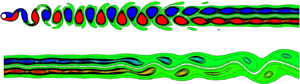
The time evolution of the vortices at Re = 160 was completely different from that at Re = 200. Detailed time evolution of the vortices at Re = 160 was examined for a time period of t* = 2500–3370, and is illustrated in figure 6 with the instantaneous vorticity field at a typical time instant t* = 3000. For Re = 160, the two-layered vortices were annihilated into two parallel shear layers with no vortices at x/D ~ 130 (figure 6a), which was different from the case at Re = 200 where the two-layered vortices merged and resulted in the secondary vortex street. It was also found that individual vortices would always reoccupy the entire parallel shear layers at locations further downstream of $x/D\mathrm{\ \mathbin{\lower.3ex\hbox{$\buildrel\gt \over {\smash{\scriptstyle\sim}\vphantom{_x}}$}}\ }320$ (e.g. figure 6c). The disappearance and reappearance of the vortices in the parallel shear layers indicated that the reappeared vortices certainly did not arise from the merging of the two-layered vortices. Instead, the hydrodynamic instability of the parallel shear layers induced flapping/waviness of the bare shear layers (i.e. shear layers with no vortices), which eventually triggered the reappearance of the vortices in the shear layers. The reappeared vortices did not emerge at a particular streamwise location. Instead, the reappearance spanned a long range of x/D ~ 140–320. For example, in figure 6(b), the parallel shear layers were only partly occupied by the reappeared vortices at x/D ~ 190–205, while the bare shear layers at x/D ~ 175–190 remained in this pattern for approximately another 50D before vortices reappeared.

Figure 6. Instantaneous vorticity field for Re = 160 at a typical time instant of t* = 3000. The vorticity field is shown for (a) x/D = 120–140 with |ω| = 0.11–0.14, (b) x/D = 175–205 with |ω| = 0.07–0.10 and (c) x/D = 350–390 with |ω| = 0.03–0.045.

Compared with the secondary vortices of Re = 200 shown in figure 5, the reappeared vortices at Re = 160 (e.g. figure 6c) were much weaker in strength, such that they largely remained in the two shear layers. Figure 7(a) shows the spatial distribution of the vortex centres for Re = 160 at t* = 3000. After the transition to the two-layered vortex street at x/D ~ 30, the positive and negative vortices followed two clear linear pathways (i.e. the two shear layers) up to the downstream extent of the computational domain, which indicated that the reappeared vortices stayed in the two shear layers. This was in contrast to the irregular spatial distribution of the vortices at Re = 200 (figure 5).

Figure 7. Vortex patterns for Re = 160 at the time instant t* = 3000: (a) spatial distribution of the vortex centres and (b) evolution of the spatial scale of the vortices with distance downstream.

Nevertheless, the spatial scale of the reappeared vortices was larger than that of the primary and two-layered vortices. The spatial scale of the vortices was quantified in figure 7(b) by the streamwise distance between the centres of the two adjacent same-sign vortices (denoted λ). As shown in figure 7(b), the λ/D values for the reappeared vortices were roughly twice those of the primary and two-layered vortices. Figure 7(b) also shows the λ/D values for the primary and secondary vortices observed experimentally by Taneda (Reference Taneda1959) at a similar Re of 149, whose results, although not detailing the fluctuations in λ/D for the secondary vortices, were largely consistent with the present results. To be consistent with Taneda (Reference Taneda1959), who found that the main feature of the secondary vortices is a spatial scale larger than the primary vortices, in the present study, the reappeared vortices observed at Re = 160 were considered as secondary vortices, although they were relatively weak and remained in the two shear layers.

3.3. Both FM1 and FM2 for intermediate Re of 170–180

Detailed time evolution of the vortices at Re = 170 was examined for a time period of t* = 2400–2800. In general, the two-layered vortices were annihilated into two bare shear layers at x/D ~ 120, which was similar to that shown in § 3.2 for Re = 160. An exception was that for a short time period of t* = (2400 + 54T*)–(2400 + 62T*), vortex merging similar to that of Re = 200 (§ 3.1) was observed over a range of x/D ~ 100–120 (see figure 8a). The vortices shown in figure 8(a) included four positive and four negative merging cycles as well as a negative single vortex (i.e. negative vortex 5). The merged vortices were not annihilated because their spatial scales were enlarged. In addition, the spatial scale of the single vortex 5 was also enlarged by the waviness of the shear layers induced by the vortex merging at the two sides of this vortex. These enlarged vortices were clearly identified as the secondary vortices as they propagated further downstream (figure 8b–d). The waviness of the two shear layers at the two sides of the group of the secondary vortices excited additional vortices, for example, positive vortex 9 and negative vortex 10 shown in figure 8(c). However, the relatively weak vortices in the range of x/D ~ 250–350 in figure 8(c) that remained in the two shear layers were similar to those observed at Re = 160 (see e.g. figure 6c) and were excited by the instability and flapping of the bare shear layers. In figure 8(d), as the group of the secondary vortices propagated further downstream, more vortices were excited at its two sides, which arose from the combined effects of (i) the increased waviness of the two shear layers induced by the further enlarged secondary vortices as they propagated downstream; and (ii) intrinsic instability of the shear layers.

Figure 8. Time evolution of the secondary vortices at Re = 170. The same vortices that appear in different snapshots are labelled with the same numbers. The labels above and below the vortices correspond to the negative and positive vortices, respectively.

The detailed time evolution of the vortices at Re = 180 was examined for time periods of t* = 2000–2360 and 2900–3100. In general, the two-layered vortices merged into secondary vortices over a range of x/D ~ 90–110, which was similar to that shown in § 3.1 for Re = 200. An exception was that for a short time period of t* = (2900 + 13T*)–(2900 + 21T*), the two-layered vortices were annihilated into two bare shear layers at x/D ~ 113, which was similar to that shown in § 3.2 for Re = 160. New vortices were excited from these fractions of bare shear layers downstream at x/D ~ 115–140.

5.1. Characteristics of the shear layers in the intermediate wake

Kumar & Mittal (Reference Kumar and Mittal2012) investigated the intermediate and far wake of Re = 150 and characterised the hydrodynamic instability in FM1 as a convective instability. This study will show that convective instability is responsible for the emergence of the secondary vortices for all Re values, regardless of its manifestation through FM1 or FM2.

It is well known that the rearrangement of the vortices from the primary vortex street to the two-layered vortex street would divert the flow away from the wake centreline and result in a ‘calm region’ near the wake centreline (in between the two layers of vortices) where the streamwise velocity is relatively small (Durgin & Karlsson Reference Durgin and Karlsson1971). The present results showed that the transition to the two-layered vortex street occurred at around x/D = 26–29 (corresponding to local maxima of u_y) for Re = 140–200, and correspondingly, the u_x value sampled along the wake centreline decreased over x/D ~ 20–40 (figure 10a). Figure 10(a) also shows that with increasing Re, the velocity deficit at the wake centreline increased. Figure 10(b) illustrates the u_x profiles sampled at x/D = 40, which showed that with increasing Re, the velocity deficit increased while the wake width decreased, and both contributed to an increase in the shear rate of the two shear layers. Figure 10(c) quantifies the maximum shear rate (∂u_x/∂y)_max of the u_x profiles sampled at various x/D locations for various Re values. With the increase in Re, the maximum shear rate gradually increased, which suggested that the shear layers became increasingly convectively unstable to allow for an earlier (in terms of the streamwise location) emergence of the secondary vortices. The convective instability of the shear flow for the present case was similar to the well-known Kelvin–Helmholtz instability for the plane mixing layer (e.g. Drazin Reference Drazin1970; Brown & Roshko Reference Brown and Roshko1974; Rogers & Moser Reference Rogers and Moser1992) and the separating shear layer of a cylinder (e.g. Prasad & Williamson Reference Prasad and Williamson1997).

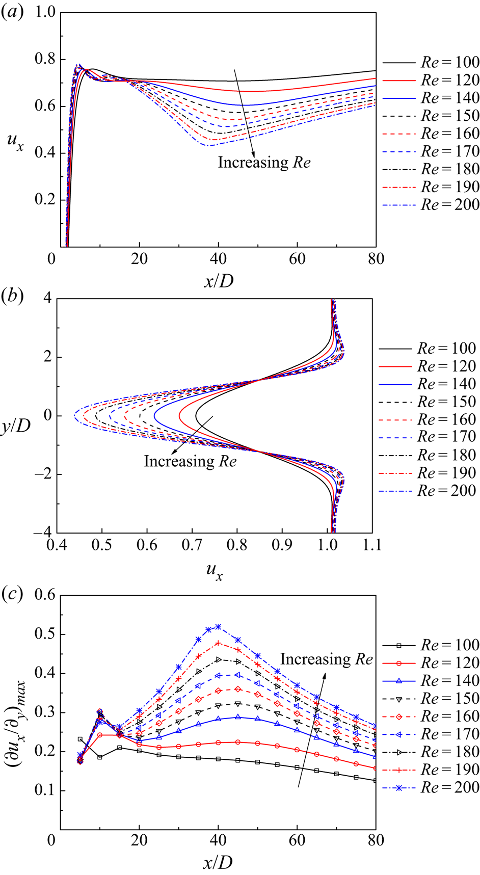
Figure 10. Characteristics of the u_x profiles for various Re values: (a) the u_x profiles sampled along the wake centreline, (b) the u_x profiles sampled at x/D = 40 and (c) the maximum shear rate of the u_x profiles sampled at various x/D locations.

5.2. Transient growth analysis of the intermediate wake

To investigate the Re-dependence of the shear-layer characteristics in the intermediate wake (which is responsible for the Re-dependence of the emergence of the secondary vortices) more quantitatively, transient growth analysis was adopted in this section to quantify the maximum growth of the perturbation energy in the time-averaged wake. The transient growth analysis was performed for Re = 100–200, which enabled an examination of the Re-dependence of the maximum growth. In addition, the range of Re = 100–200 incorporates both FM1 and FM2, and this range will be examined if convective instability is shown to be the universal underlying mechanism.

Figure 11 summarises the optimal energy growths G(τ) calculated under various combinations of τ and Re. As shown in figure 11, the transient energy growths for different Re values shared similar qualitative trends, which suggested that there was no fundamental difference among the different Re values. Therefore, the massive amplification of the perturbation energy was a prerequisite for the emergence of the secondary vortices for all Re values, regardless of their manifestation through FM1 or FM2.

Figure 11. Optimal energy growth G(τ) as a function of the time interval τ for various Re values.

Figure 12 illustrates further the results of Re = 180 as an example, where the curve G(τ) − τ is reproduced from figure 11. Also shown in figure 12 are the linear energy growths E(t*)/E(0) evolved from the optimal initial perturbations for various τ values. Based on an additional case with τ = 60 and a reduced domain size up to x/D = 300, it was confirmed that the time evolution of the linear energy growth was unaffected by the location of the outlet boundary (until the perturbation was washed out of the domain). Naturally, each energy growth curve shown in figure 12 osculated the optimal growth curve G(τ) − τ at t* = τ, i.e. the optimal growth curve was the envelope of the energy growth curves for various τ (Blackburn, Barkley & Sherwin Reference Blackburn, Barkley and Sherwin2008). In addition, the energy growth curves for relatively large τ values (e.g. τ = 100 and 200) corresponded approximately quantitatively to the envelope. Therefore, the energy growth for the case τ = 100 or 200 may serve as an approximation of the optimal energy growth in a time evolution manner.

Figure 12. Optimal energy growth curve log₁₀G(τ) − τ for Re = 180, together with the linear energy growths E(t*)/E(0) evolved from the optimal initial perturbations for various τ values.

The energy growth for the case τ = 100 is further shown in figure 13 by the time evolution of the linear perturbation vorticity field. The case τ = 100 was chosen because it produced the optimal energy growth G(τ) at t* = τ = 100 and corresponded to x/D ~ 80–120 (figure 13b), which was close to the range of x/D for the emergence of the secondary vortices (x/D ~ 90–140 in figure 9). To show clearly the initial evolution of the perturbation, the vorticity fields in figure 13(a) were plotted with a vorticity range 100 times smaller than that used in figure 13(b). The time evolution of the linear perturbation vorticity field shown in figure 13 was consistent with the energy growth trend of τ = 100 shown in figure 12, where a massive energy amplification was observed for t* up to approximately 300, followed by a gradual energy decay afterwards. This observation confirmed that the flow was globally stable but locally convectively unstable.

Figure 13. Time evolution of the linear perturbation vorticity field developed from the optimal initial perturbation for Re = 180 and τ = 100. The linear perturbation vorticity fields are symmetric about the wake centreline. Positive and negative vorticity values are in red and blue, respectively. The range of vorticity in panel (a) for t* = 0–50 is 100 times smaller than the range in panel (b) for t* = 50–400. In panel (a), the vertical line at x/D = 10 represents the left end of the domain.

It is interesting to note that the optimal initial perturbation shown in figure 13(a) (at t* = 0) shared close similarity to the two-dimensional optimal initial perturbations for plane Poiseuille, Couette and backward-facing step flows, where a series of highly strained counter-rotating rollers are observed and their inclination is opposite to the direction of the mean shear (Farrell Reference Farrell1988; Butler & Farrell Reference Butler and Farrell1992; Blackburn, Barkley & Sherwin Reference Blackburn, Barkley and Sherwin2008). The mean shear for the channel flows, such as the plane Poiseuille and backward-facing step flows, was in an opposite direction to that of the present wake flow, and, therefore, so was the inclination of the perturbation rollers. The fundamental similarity of the initial perturbation structures for all of these flows confirmed that the transient energy growth of the present wake flow also arose from the mean shear, as discussed earlier in § 5.1.

It was also seen in figure 13(a) that, with the evolution in time, the upper and lower rows of the counter-rotating rollers quickly interacted and formed an integrated pattern, which suggested interactions of the two shear layers. The integrated pattern stabilised at ${t^\ast }\mathrm{\ \mathbin{\lower.3ex\hbox{$\buildrel\gt \over {\smash{\scriptstyle\sim}\vphantom{_x}}$}}\ }20$ and then appeared similar to that shown by Kumar & Mittal (Reference Kumar and Mittal2012).

5.3. Effect of the Reynolds number

The Re-dependence of the optimal energy growth is quantified in figure 11, where G(τ) increased noticeably with the increase in Re. For example, an increase in Re by 20 resulted in an increase in G(150) of approximately one order of magnitude. The dependence of G(τ) on Re suggested that the wake was increasingly convectively unstable at increasing Re values. Consequently, with the increase in Re, the secondary vortices emerged at decreasing x/D values (figure 9).

The effect of G(τ) on the x/D for the emergence of the secondary vortices was further analysed as follows. To facilitate analysis of the time evolution of the perturbation, the optimal energy growth curve G(τ) − τ for each Re, as shown in figure 11, was approximated by the linear energy growth curve [E(t*)/E(0)] − t* evolved from the optimal initial perturbation for τ = 200 (figure 14), because the two curves are quantitatively similar (e.g. figure 12). To generate a link between the energy growth over t* and that over x/D, the streamwise advection of the perturbation for τ = 200 was quantified by the movement of the centroidal location of the perturbation energy (x_c/D) over time (figure 15a), where x_c is calculated as

(5.1)\begin{equation}{x_c} = \frac{\displaystyle{\int_\Omega {\tfrac{1}{2}(u^{\prime 2}_x + u^{\prime 2}_y)x\,\textrm{d}\varOmega } }}{\displaystyle{\int_\Omega {\tfrac{1}{2}(u^{\prime 2}_x + u^{\prime 2}_y)\,\textrm{d}\Omega } }}.\end{equation}

In addition, figure 15(b) shows that the advection velocity of x_c/D was not a constant. As illustrated by an example at Re = 150, the variation of the advection velocity with distance downstream qualitatively followed the trend of the time-averaged streamwise velocity profile sampled along the wake centreline (while the quantitative difference in the velocity was because the velocity deficit at the wake centreline was the largest).

Figure 14. Linear energy growth E(t*)/E(0) evolved from the optimal initial perturbation for τ = 200.

Figure 15. Movement of the centroidal location of the perturbation energy over time for τ = 200 and various Re: (a) the relationship between x_c/D and t* and (b) the advection velocity of x_c/D as a function of x_c/D.

Based on the relationship between x_c/D and t* shown in figure 15(a), the linear energy growth curve [E(t*)/E(0)] − t* shown in figure 14 was transformed into [E(t*)/E(0)] − (x_c/D) in figure 16. Figure 16 also highlights (in the thick segment of the curve) the range of x/D for the emergence of the secondary vortices (previously shown in figure 9). The secondary vortices generally emerged at energy amplification levels of 10⁵–10⁷. This observation suggested that, with the increase in Re, the increasing gradient in the energy amplification was responsible for the emergence of the secondary vortices at decreasing x/D and for a decreasing range of x/D, both of which were shown originally in figure 9.

Figure 16. Linear energy growth E(t*)/E(0) evolved from the optimal initial perturbation for τ = 200, with the horizontal axis being transformed from t* to x_c/D.

In addition, table 3 lists the transient growth analyses performed with different base flows. Cases 1 and 2 were computed conventionally, where the base flow and the transient growth analysis were computed with the same Re value. In contrast, the transient growth analyses of cases 3 and 4 were computed with a base flow obtained from a different Re. The purpose of cases 3 and 4 was to show that the G(τ) value was, to a great extent, dictated by the base flow, i.e. the shear-layer characteristics investigated in § 5.1.

Table 3. Optimal energy growths computed with different base flows.

5.4. Effect of the interaction of the two shear layers

Interactions of the two shear layers were observed both in the relatively far wake (where the secondary vortices emerge) and in the intermediate wake (where the transient growth develops). The flow visualisation in § 3 suggested that the formation of the secondary vortices (through either FM1 or FM2) was a result of the interaction/flapping of the two parallel shear layers at similar streamwise locations, where positive and negative secondary vortices emerged simultaneously (see e.g. figures 4, 6b and 8a). In addition, the modified case of Re = 200 investigated in § 4 (with an artificial horizontal slip plate of zero-thickness placed at the wake centreline and x/D ≥ 80) showed that by eliminating the interaction between the two shear layers at x/D ≥ 80, the secondary vortices were suppressed over the entire wake for x/D up to 400. Furthermore, the linear perturbation vorticity fields shown in figure 13 displayed interactions of the upper and lower rows of the rollers as early as t* = 5. Kumar & Mittal (Reference Kumar and Mittal2012) also showed that by altering the perturbation modes through placing a slip plate at the wake centreline over x/D = 27.5–62.5, the oscillations in the far wake became significantly weaker.

To quantify the effect of the interaction of the two shear layers, additional transient growth analysis was conducted by using only the lower half of the computational domain (where the top boundary for the perturbation adopted the slip condition). The base flow for the half domain was mapped from, and thus identical to, the lower half of the time-averaged base flow for the full domain. Because the base flow for the full domain was symmetric about the wake centreline, the transient energy growth predicted based on the lower half of the domain was the same as that predicted based on a full domain but with a slip plate placed at the wake centreline. In this case, all possible interactions between the two shear layers were eliminated, while the characteristics of the individual shear layer remained strictly unchanged.

Figure 17 shows the optimal energy growths G(τ) for Re = 200 predicted based on the full domain and half domain. The G(τ) values predicted by the full domain were significantly larger than the half-domain counterparts, which suggested that the interaction of the two shear layers significantly promoted the transient energy growth (hence, played an important role in the formation of the secondary vortices). The G(τ) values predicted by the half domain were well below the threshold of ~ 10⁵ for the emergence of the secondary vortices.

Figure 17. Optimal energy growths G(τ) for Re = 200 predicted based on the full domain and half domain.