2.1. The minimal flow unit

The flow case chosen is that explored by Hamilton et al. (Reference Hamilton, Kim and Waleffe1995). It is defined by the smallest box and the smallest Reynolds number in which turbulence can be sustained without any external forcing. For Couette flow, the minimal box has dimensions $(L_x,L_y,L_z)=(1.75{\rm \pi} h,2h,1.2{\rm \pi} h)$, denoting lengths in the streamwise, wall-normal and spanwise directions, respectively; $h$ is the channel half-height. Plane Couette flow is realisable in experiments (Tillmark & Alfredsson Reference Tillmark and Alfredsson1992; Bech et al. Reference Bech, Tillmark, Alfredsson and Andersson1995; Bottin & Chaté Reference Bottin and Chaté1998). Numerical simulations with sufficiently large domains lead to statistics matching experiments (Komminaho, Lundbladh & Johansson Reference Komminaho, Lundbladh and Johansson1996). Minimal domains such as the present one have qualitative agreement with experimental results (see, for instance, Jiménez & Moin (Reference Jiménez and Moin1991) for an early example with channel flow), but greatly simplify the analysis; because of this, such small domains are often used in dynamical-system descriptions of turbulent flows (Kawahara & Kida Reference Kawahara and Kida2001; Waleffe Reference Waleffe2003; Gibson, Halcrow & Cvitanović Reference Gibson, Halcrow and Cvitanović2009). The discretisation was chosen as $(n_x,n_y,n_z)=(32,65,32)$ before dealiasing in the wall-parallel directions, which gives a slightly higher resolution than that used in Hamilton et al. (Reference Hamilton, Kim and Waleffe1995). We consider Couette flow with walls moving at velocity $\pm U_w$; the Reynolds number for this case is $Re=400$, based on wall velocity $U_w$ and half-height $h$. For this flow, this leads to a friction Reynolds number $Re_\tau \approx 34$, based on the friction velocity. From now on, all quantities are non-dimensional values based on outer units, with $h$ and $U_w$ as reference length and velocity. The simulation is performed in SIMSON, a pseudo-spectral solver for incompressible flows (Chevalier, Lundbladh & Henningson Reference Chevalier, Lundbladh and Henningson2007), with discretisation in Fourier modes in streamwise and spanwise directions, and in Chebyshev polynomials in the wall-normal direction.

The simulation is initialised with white noise in space for $Re=625$, which becomes turbulent after a few timesteps; the Reynolds number is, then, slowly decreased until the desired value of $400$. After reaching the desired value of $Re$ and discarding initial transients, flow fields are stored every ${\rm \Delta} t=0.5$ in the interval $10\,000 < t < 25\,000$. During this period, several streak regeneration cycles are observed, and the flow is expected to be statistically stationary. The mean turbulent velocity profile is shown in figure 1(a), which has the usual ‘$S$’ profile typical of turbulent Couette flow. The mean profile and fluctuation levels match previous results for the same computational domain and Reynolds number (Gibson, Halcrow & Cvitanović Reference Gibson, Halcrow and Cvitanović2008). 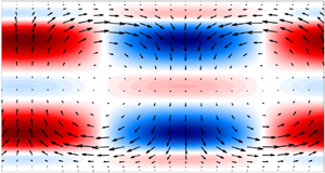A snapshot of the streamwise velocity fluctuations for a $(\kern-0.05em y,z)$ plane is shown in figure 1(b). As expected, streaks arise clearly in the velocity field, since these structures are the most relevant in the turbulent dynamics of this sheared flow; they are flanked by streamwise vortices with the expected lift-up behaviour: positions with downward/upward motion display lifted high/low momentum, leading to a high/low-speed streak.

Figure 1. Mean velocity for Couette flow and snapshot of the velocity field in the $(\kern-0.05em y,z)$ plane (colours: streamwise velocity; arrows: spanwise and wall-normal velocities). (a) Mean flow and (b) snapshot of velocity field.

Using the results from the direct numerical simulation (DNS), the velocity fluctuations around the mean-flow profile (treated as response of the input–output version of the Navier–Stokes system) were computed; these, in turn, were used to compute the nonlinear terms of the Navier–Stokes equations, which will be treated as a forcing term in the Navier–Stokes equations expanded around the mean flow. These are computed directly as a function of time in the physical domain. After that, the resulting forcing was Fourier transformed in space, leading to forcings as a function of streamwise and spanwise wavenumbers, but still in the time domain. Using the forcing and velocity in the time-wavenumber domain, we computed the CSDs of the response (${\boldsymbol {S}}$) and of the forcing (${\boldsymbol {P}}$). This is further detailed in the next section.

2.2. Recovering response statistics from the forcing CSD

Since Couette flow is homogeneous in $x$ and $z$ directions, the first step for the analysis of this flow is to perform a spatial Fourier transform of both response and forcing, so the analysis can be performed separately for each wavenumber. Modes are defined by the integers $(n_\alpha ,n_\beta )$, with $\alpha =2 {\rm \pi}n_\alpha /L_x$ and $\beta =2 {\rm \pi}n_\beta /L_z$ being the wavenumbers, following the same notation of Hamilton et al. (Reference Hamilton, Kim and Waleffe1995). The wall-normal integrated kinetic energy of the first two modes, some of the most relevant ones in the analysis of Hamilton et al. (Reference Hamilton, Kim and Waleffe1995), is shown in figure 2, showing the fluctuations peak at vanishing frequency $\omega \to 0$ for mode $(0,1)$, and a plateau is observed at low frequencies for mode $(1,0)$. Since we consider a Couette flow with walls moving at opposite velocities, $\pm U_w$, this very low-frequency behaviour reflects that the two modes peak at approximately zero phase speed, without preferred motion following some streamwise or spanwise direction, as can be induced from the results of Hamilton et al. (Reference Hamilton, Kim and Waleffe1995). The time power spectral density (PSD) for each mode was estimated using the Welch method, with the signal divided in segments of $n_{fft}=1024$ with $75\,\%$ overlap, which led to 114 blocks for the analysis. A Hanning window was used to reduce spectral leakage, allowing accurate relation between forcing and response of the system.

Figure 2. Power spectral density of the wall-normal integrated kinetic energy for the different modes studied herein.

We will study the two most energetic modes at low frequencies, as showed in Hamilton et al. (Reference Hamilton, Kim and Waleffe1995): mode $(0,1)$, which is related to the appearance of streaks; and mode $(1,0)$, which emerge once the amplitude of mode $(0,1)$ decreases, characterising streak breakdown (Hamilton et al. Reference Hamilton, Kim and Waleffe1995). Applying the Reynolds decomposition, we will consider an expansion around the mean flow, averaged over streamwise and spanwise directions and in time, so that each component of the velocity can be written as the sum of mean and fluctuation fields ($U_i+\tilde {u}_i$), with $U_i$ denoting the mean velocity profile and the tilde indicating fluctuations in time domain. Thus, we can write the incompressible Navier–Stokes equations for the fluctuations as

(2.1)\begin{equation} \frac{\partial \tilde{u}_i}{\partial t} + U_j \frac{\partial \tilde{u}_i}{\partial x_j} + \tilde{u}_j \frac{\partial U_i}{\partial x_j} = -\frac{\partial \tilde{p}}{\partial x_i} + \frac{1}{Re}\frac{\partial^2 \tilde{u}_i}{\partial x_j \partial x_j} + \tilde{f}_i, \end{equation}

and the continuity equation

(2.2)\begin{equation} \frac{\partial \tilde{u}_i}{\partial x_i}=0, \end{equation}

where Einstein summation is implied, $\tilde {u}_i$ are the three velocity components, $\tilde {p}$ is the pressure and the forcing term $\tilde {f}_i$ is considered to gather the nonlinear terms of the Navier–Stokes equations,

(2.3)\begin{equation} \tilde{f}_i = -\tilde{u}_j\partial \tilde{u}_i/\partial x_j + \overline{\tilde{u}_j\partial \tilde{u}_i/\partial x_j},\end{equation}

where $\overline {\tilde {u}_j\partial \tilde {u}_i/\partial x_j}$ is the mean Reynolds stress, which is only be present in the zero-frequency/zero-wavenumber equation (i.e. the mean-flow equation, which is the Reynolds averaged Navier–Stokes equation). Taking the Fourier transform in $x$, $z$ and $t$, and considering that the mean flow has only the streamwise component $U(\kern-0.05em y)$, leads to

(2.4a)\begin{gather} -\textrm{i} \omega u + \textrm{i} \alpha U u + v \frac{\partial U}{\partial y} = -\textrm{i} \alpha p + \frac{1}{Re}\left(-\alpha^2-\beta^2+\frac{\partial^2}{\partial y^2}\right) u + f_x, \end{gather}

(2.4b)\begin{gather}-\textrm{i} \omega v + \textrm{i} \alpha U v = -\frac{\partial p}{\partial y} + \frac{1}{Re}\left(-\alpha^2-\beta^2+\frac{\partial^2}{\partial y^2}\right) v + f_y, \end{gather}

(2.4c)\begin{gather}-\textrm{i} \omega w + \textrm{i} \alpha U w = -\textrm{i} \beta p + \frac{1}{Re}\left(-\alpha^2-\beta^2+\frac{\partial^2}{\partial y^2}\right) w + f_z, \end{gather}

(2.4d)\begin{gather}\textrm{i} \alpha u + \frac{\partial v}{\partial y} + \textrm{i} \beta w =0, \end{gather}

where $\omega$ is the frequency, $(u,v,w,p)$ are the Fourier transformed perturbation quantities and $(f_x,f_y,f_z)$ the Fourier transforms of $\tilde {f}_i$. From the equations above, we can write the incompressible Navier–Stokes equations for the perturbations in the wavenumber and frequency domain in an input–output form as

(2.5)\begin{equation} -\textrm{i} \omega {\boldsymbol{H}} \boldsymbol{q} ={\boldsymbol{A}} \boldsymbol{q} + \boldsymbol{f}\!, \end{equation}

where $\boldsymbol {q} =[u \ v \ w \ p]^{\textrm {T}}$ is the output and $\boldsymbol {f}=[f_x \ f_y \ f_z \ 0]^{\textrm {T}}$ is the forcing term (input). The matrix ${\boldsymbol {A}}$ is the linear operator defined by Navier–Stokes and continuity equations (which is a function of the streamwise and spanwise wavenumbers $\alpha$ and $\beta$) and the matrix ${\boldsymbol {H}}$ is defined to zero the time derivative of the pressure. This can be rewritten in the usual resolvent form:

(2.6)\begin{gather} (-\textrm{i} \omega {\boldsymbol{H}} - {\boldsymbol{A}}) \boldsymbol{q} = \boldsymbol{f}\!, \end{gather}

(2.7)\begin{gather}\Rightarrow {\boldsymbol{L}} \boldsymbol{q} = \boldsymbol{f}\!, \end{gather}

(2.8)\begin{gather}\Rightarrow \boldsymbol{q} = {\boldsymbol{L}}^{-1} \boldsymbol{f} = {\boldsymbol{R}} \boldsymbol{f}\!. \end{gather}

With the equations written in this shape, optimal forcings and responses (in the linear framework, based on linearisation of the Navier–Stokes equations around the mean flow) can be obtained for a turbulent flow by performing a singular value decomposition of the resolvent operator, which leads to orthogonal bases for responses $\boldsymbol {q}_i$ and forcings $\boldsymbol {f\!}_i$, related by gains $s_i$. The singular value decomposition considers the weighting matrix corresponding to Clenshaw–Curtis quadrature associated to the Chebyshev weights in the present grid (Trefethen Reference Trefethen2000).

Optimal response and the respective gain from resolvent analysis are directly comparable to the most energetic structures in the flow if the forcing is considered to be statistically white in space (Towne et al. Reference Towne, Schmidt and Colonius2018a). In order to consider the actual statistics of the flow in this framework, we define the covariance matrices of the response ${\boldsymbol {S}}=\mathcal {E}(\boldsymbol{q q}^H)$ and of the forcing ${\boldsymbol {P}}=\mathcal {E}(\,\boldsymbol{f f}^H)$, and $\mathcal {E}$ representing the expected value of a signal, which is computed by averaging realisations in the Welch method (taking the block average of $\boldsymbol {q} \boldsymbol {q}^H$ as a function of frequency). Following Towne et al. (Reference Towne, Schmidt and Colonius2018a) and Cavalieri et al. (Reference Cavalieri, Jordan and Lesshafft2019), these quantities are related via

(2.9)\begin{equation} \left.\begin{gathered} \boldsymbol{q} \boldsymbol{q}^H = {\boldsymbol{R}} \boldsymbol{f} \boldsymbol{f}^H {\boldsymbol{R}}^H, \\ \mathcal{E}(\boldsymbol{q} \boldsymbol{q}^H) = {\boldsymbol{R}} \mathcal{E}(\boldsymbol{f} \boldsymbol{f}^H) {\boldsymbol{R}}^H, \\ {\boldsymbol{S}}={\boldsymbol{R}} {\boldsymbol{P}} {\boldsymbol{R}}^H. \end{gathered}\right\} \end{equation}

If it is assumed that the covariance of the forcing is uncorrelated in space then ${\boldsymbol {P}} = \mathrm {I}$ and the covariance of the response is given by ${\boldsymbol {S}}={\boldsymbol {R}} {\boldsymbol {R}}^H$. Therefore, if the statistics of the forcing follows this hypothesis, the spectral proper orthogonal decomposition (SPOD) modes, defined by the eigenfunctions of

(2.10)\begin{equation} \int_{-1}^1 {\boldsymbol{S}}(\kern-0.05em y,y',\omega) \boldsymbol{q}_{SPOD}(\kern-0.05em y',\omega)\,\textrm{d} y' = \sigma \boldsymbol{q}_{SPOD}(\kern-0.05em y,\omega) \end{equation}

are identical to response modes (left singular vectors of ${\boldsymbol {R}}$). For more details on this derivation, the reader should refer to Towne et al. (Reference Towne, Schmidt and Colonius2018a) and Cavalieri et al. (Reference Cavalieri, Jordan and Lesshafft2019). As in the computation of resolvent modes, SPOD modes are computed numerically with the inclusion of integration weights (Schmidt et al. Reference Schmidt, Towne, Rigas, Colonius and Brès2018), such that flow structures resulting from both analyses can be directly compared with each other.

However, non-white forcing covariance (which must be the case in turbulent flows) must be included in the formulation in order to correctly educe the response statistics. The inclusion of ${\boldsymbol {P}}$ can be done in several ways. One of them is to directly compute the nonlinear terms of the Navier–Stokes equations from simulation data. Other approaches include modelling the forcing starting from specific assumptions on the flow case (Moarref et al. Reference Moarref, Sharma, Tropp and McKeon2013), its identification from limited flow information (Zare et al. Reference Zare, Jovanović and Georgiou2017; Towne, Yang & Lozano-Durán Reference Towne, Yang and Lozano-Durán2018b), and modelling by means of an eddy viscosity included in the linear operator (Tammisola & Juniper Reference Tammisola and Juniper2016; Morra et al. Reference Morra, Semeraro, Henningson and Cossu2019).

The present work focuses on exploring different forcing covariances and their effect on the covariance of the response. The first approach is to simply consider the forcing to be uncorrelated in space; for this case, previous analyses for wall-bounded flows has shown that even though reasonable agreement may be obtained for near-wall fluctuations (Abreu et al. Reference Abreu, Cavalieri, Schlatter, Vinuesa and Henningson2019), a mismatch is observed for large-scale structures (Morra et al. Reference Morra, Semeraro, Henningson and Cossu2019). One can also compute the nonlinear terms directly from a numerical simulation and then determine accurately ${\boldsymbol {P}}$. If the simulation is converged and the signal processing is done properly, the result of (2.9) using the actual forcing covariance ${\boldsymbol {P}}$ (in the sense that this quantity is directly obtained from the simulation) should be equal to the response covariance ${\boldsymbol {S}}$ computed from the same simulation.

3.1. Connection between forcing and response statistics: role of the correction due to windowing

Although (2.9) is exact, if ${\boldsymbol {P}}$ and ${\boldsymbol {S}}$ are estimated from a finite set of data, large errors arise in the velocity statistics recovery process using the resolvent operator, leading to non-negligible values for ${\boldsymbol {S}}-{\boldsymbol {R}}{\boldsymbol {P}}{\boldsymbol {R}}^H$. From the analysis of Martini et al. (Reference Martini, Cavalieri, Jordan and Lesshafft2019) (summarised in appendix A for the present case), application of windowing in the data (which is necessary for applying Welch's method) generates extra force-like terms that must be accounted to have the correct input–output relation, so that (2.9) holds for the estimated covariances. The impact of these extra terms can be measured as

(3.1)\begin{equation} Error = \frac{||{\boldsymbol{S}}_{rec} - {\boldsymbol{S}}||}{||{\boldsymbol{S}}||}, \end{equation}

where ${\boldsymbol {S}}_{rec}$ is the covariance of the response recovered from the statistics of the forcing using (2.9), applied for both uncorrected and corrected forcing terms; the norm was chosen as the standard 2-norm for matrices. Similarly, the effect of the correction on the covariance of the forcing can be evaluated by the metric

(3.2)\begin{equation} \epsilon=\frac{||{\boldsymbol{P}}_{DNS+c}-{\boldsymbol{P}}_{DNS}||}{||{\boldsymbol{P}}_{DNS+c}||}, \end{equation}

where ${\boldsymbol {P}}_{DNS}$ denotes the covariance of the forcing obtained from the simulation without correction, and ${\boldsymbol {P}}_{DNS+c}$ denotes the corrected covariance. With these metrics, we can evaluate how this correction term affects the process of recovering ${\boldsymbol {S}}$ from ${\boldsymbol {P}}$. The comparison of the errors with and without this correction term is shown in figure 3(a) for the two Fourier modes studied in this work.

Figure 3. Effect of the correction term in the recovery of ${\boldsymbol {S}}$ and on the forcing covariance ${\boldsymbol {P}}$. Spectra normalised by ${\rm \Delta} \omega$. (a) Response CSDs error norm and (b) influence on ${\boldsymbol {P}}$.

From figure 3(a), we can see that the correction affects a wide range of frequencies, with a slightly lower effect in higher frequencies. Following Martini et al. (Reference Martini, Cavalieri, Jordan and Lesshafft2019), we can divide the aliasing error into two components: the first is due to spectral content at frequencies higher than the Nyquist frequency, and the other is due to the window spectral leakage, which generates extra content above the Nyquist frequency. Only the latter can be reduced with a proper choice of windowing function. The aliasing behaviour of the error explain the larger errors obtained at higher frequencies in figure 3(a), and indicates that the first type of aliasing is dominant in that region. As this work will focus on the study of low-frequency structures, no further effort is made in order to reduce the error in higher frequencies; moreover, since the normalised errors are below $10^{-4}$ in all cases, an optimisation of the window was deemed unnecessary for our purposes.

A similar trend is found for the influence of the correction on the covariance of the forcing, shown in figure 3(b). The correction strongly affects the lower frequency region, but most of this covariance is still dominated by the nonlinear terms of the Navier–Stokes equations. As $\epsilon$ is only a fraction of the overall forcing, it is thus meaningful to study the forcing covariance ${\boldsymbol {P}}$ in an attempt to simplify it, keeping in mind that once predictions of the response ${\boldsymbol {S}}$ are needed one needs to account for the correction term.

The correction greatly improves the recovery process for all modes, leading to a reduction of the error of about five orders of magnitude for the two considered modes, which is possibly related to the low-order dynamics of the flow for this combination of wavenumbers, a feature that will be further explored in §§ 4.1 and 4.2. The effect of the correction on the shapes of each case will be studied in the next section.

The role of the forcing terms is studied throughout this work. All the comparisons between forces and responses will implicitly consider the correction term, unless otherwise stated. In all other contexts ‘external force’ will refer only to the term $\boldsymbol {f}\!$, without considering the correction term.

3.2. Comparison with statistics from white-noise forcing and no correction

Here, we analyse the effect of the different choices of forcing CSDs ${\boldsymbol {P}}$ on the velocity statistics. As stated previously, we focus on very low frequencies in order to evaluate the effect of the statistics of the nonlinear terms on the most energetic streaks, and on the equivalent structures for other combinations of wavenumbers. For that reason, we choose $\omega =0.0123$ for the analysis of modes $(0,1)$ and $(1,0)$; this is the first non-zero frequency from the Welch method for the present case (this frequency can be seen as the limit $\omega \to 0$ in this analysis). This frequency was chosen so as to analyse the behaviour of the very large, almost time-invariant structures observed in the minimal flow unit. Analogous structures have been identified by a number of authors (Komminaho et al. Reference Komminaho, Lundbladh and Johansson1996; Tsukahara, Kawamura & Shingai Reference Tsukahara, Kawamura and Shingai2006; Pirozzoli, Bernardini & Orlandi Reference Pirozzoli, Bernardini and Orlandi2011, Reference Pirozzoli, Bernardini and Orlandi2014; Lee & Moser Reference Lee and Moser2018) for turbulent Couette flow at higher Reynolds numbers. For the present low Reynolds number, these large structures have the same characteristic length of the near-wall streaks; since they have the same overall behaviour, it becomes harder to separate these in such a small box. The analysis of Rawat et al. (Reference Rawat, Cossu, Hwang and Rincon2015) indicates nonetheless that the minimal flow unit streaks become very large-scale structures in turbulent Couette flow if continuation methods are applied. Therefore, the analysis of mode $(n_\alpha ,n_\beta )=(0,1)$ should be seen as a study of the overall dynamics of the largest streaks in Couette flow.

Figure 4 shows the comparison between the absolute value of the main diagonal of ${\boldsymbol {S}}$, which corresponds to the PSD of the three velocity components. We consider the response CSD of case $(n_\alpha ,n_\beta )=(0,1)$ using the statistics of the forcing obtained from the simulation without any correction (${\boldsymbol {P}}_{DNS}$), that considering the correction term (${\boldsymbol {P}}_{DNS+c}$) and that using the white noise ${\boldsymbol {P}}=\gamma \mathrm {I}$ (with constant $\gamma$ chosen so as to match the maximum PSD for this frequency). It can be seen that the shape of the main component (streamwise velocity $u$) can be fairly well reproduced by simply using ${\boldsymbol {P}}=\gamma \mathrm {I}$. Streaks are represented, with peak amplitudes distant of about $0.4$ from the wall; this may be related to the higher shear near the walls, as shown in figure 1, leading to a stronger lift-up mechanism in that region. Considering white-noise forcing, we can see some discrepancies in the amplitudes and in some details of the shapes of the streamwise vortices ($v$ and $w$ components). Despite acknowledging the origin of the forcing terms as arising from triadic interactions, resolvent analysis as formulated by McKeon & Sharma (Reference McKeon and Sharma2010) assumes white-noise forcing statistics, predicting thus streamwise vortices and streaks that are in reasonable agreement with the DNS, although with a mismatch in the relative amplitudes of $u$, $v$ and $w$ components; similar results were obtained for turbulent pipe flow by Abreu et al. (Reference Abreu, Cavalieri, Schlatter, Vinuesa and Henningson2019). This will be explored in more detail in § 4.1. For an accurate quantitative comparison, the statistics of the nonlinear terms should be used; by doing that without the correction, the overall relative levels are closer to that from the simulation, but the amplitudes are still off, especially at the peak of each component (which explains the errors seen in figure 3). When the correction is taken into account, the exact shapes are recovered for all components, without any rescaling.

Figure 4. Response ${\boldsymbol {S}}$ from simulation and from the recovery process using different ${\boldsymbol {P}}$ (white noise, uncorrected and corrected) for case $(n_\alpha ,n_\beta )=(0,1)$. Prediction using white-noise ${\boldsymbol {P}}$ was scaled to match the maximum of ${\boldsymbol {S}}$ by the factor $\gamma =1.029\times 10^{-4}$. (a) Streamwise component, (b) wall-normal component and (c) spanwise component.

The same process was carried out for case $(1,0)$, and the results can be seen in figure 5. For this combination of wavenumbers, the flow is dominated by the spanwise velocity component, and the energy of the other velocity components are several orders of magnitude lower, as shown in figure 5. The dominance of $w$ for the (1,0) mode was also observed by Smith, Moehlis & Holmes (Reference Smith, Moehlis and Holmes2005); analysis of spectral density of turbulent channels also shows that structures with large spanwise extent are observed for $w$ (del Álamo & Jiménez Reference del Álamo and Jiménez2003). By considering white-noise statistics of the forcing, this dominance of spanwise velocity fluctuations could not be captured, and all components predicted by ${\boldsymbol {R}}{\boldsymbol {R}}^H$ have the same overall levels, leading to large errors for the $(u,v)$ components. For the spanwise component, however, the position of the peak and the shape of ${\boldsymbol {S}}$ at the centre of the domain is roughly captured by the method, even though larger errors are found for regions closer to the wall. These facts altogether point out to an action of the nonlinear terms in forcing mainly in the spanwise direction, with a more effective action closer to the wall (highlighted by the higher amplitude of the response around $y=0.4, 1.6$). By including the uncorrected statistics of the forcing, ${\boldsymbol {P}}_{DNS}$, the problem of the relative amplitudes of the different components is solved; now the spanwise component dominates the response, and its shape resembles that obtained directly from the simulation, even though a slight mismatch is found in the centre of the channel. This comparison is further improved by including the correction term in the statistics of the forcing; by using it, a perfect match between ${\boldsymbol {S}}$ computed from the simulation and the one from the forcing statistics is obtained, and the normalised error for this case is lower than $10^{-5}$.

Figure 5. Response ${\boldsymbol {S}}$ from simulation and from the recovery process using different ${\boldsymbol {P}}$ (white noise, uncorrected and corrected) for case $(n_\alpha ,n_\beta )=(1,0)$. Prediction using white-noise ${\boldsymbol {P}}$ was scaled to match the maximum of ${\boldsymbol {S}}$ by the factor $\gamma =3.6295 \times 10^{-5}$. (a) Streamwise component, (b) wall-normal component and (c) spanwise component.

4.1. Case $(n_\alpha ,n_\beta )=(0,1)$

4.1.1. Contribution of each component of the nonlinear terms

In this section we analyse more closely the structure of the nonlinear terms for the case $(0,1)$ for $\omega \to 0$ ($\omega =0.0123$). Our objective here is to look closely at the forcing statistics in order to isolate the important parts for this simple case. The number of components of the nonlinear terms, as defined in (2.3), makes an ad hoc modelling approach prohibitive; still, if only certain parts of the forcing are necessary to reproduce the statistics of the response, modelling can be considered an option. Specifically for the case $(n_\alpha ,n_\beta )=(0,1)$, the momentum equations (2.4b) and (2.4c) ($v$ and $w$) decouple from the streamwise velocity, and these equations become also independent of the mean flow $U$. That allows us to rearrange the system in order to obtain separate equations for streamwise vortices (concentrated in the $v,w$ components) and streaks (concentrated in the $u$ component) as

(4.2)\begin{align} & \underbrace{\left[-\textrm{i} \omega +\frac{1}{Re} \left(\beta^2-\frac{\partial^2}{\partial y^2}\right)\right]}_{{\boldsymbol{L}}_{01}} \underbrace{\left(\beta^2-\frac{\partial^2}{\partial y^2}\right)}_{{\boldsymbol{B}}_{01}} v = \textrm{i}\beta\left(-\textrm{i}\beta f_y+\frac{\partial f_z}{\partial y}\right) \nonumber\\ &\quad =\left(\beta^2-\frac{\partial^2}{\partial y^2}\right) f_y + \frac{\partial}{\partial y} \underbrace{\left( \frac{\partial f_y}{\partial y} + \textrm{i}\beta f_z \right)}_{\text{zero response}} \nonumber\\ &\quad \Rightarrow {\boldsymbol{L}}_{01} {\boldsymbol{B}}_{01} v={\boldsymbol{B}}_{01}\, f_y, \end{align}

(4.3)\begin{align} &\left[-\textrm{i} \omega +\frac{1}{Re}\left(\beta^2-\frac{\partial^2}{\partial y^2}\right)\right] u = f_x - v \frac{\partial U}{\partial y} \Rightarrow {\boldsymbol{L}}_{01} u = f_x - v \frac{\partial U}{\partial y}, \end{align}

where the influence of the spanwise component of the forcing is already considered in (4.2), by considering that only the solenoidal part of the forcing leads to a response in velocity; inspection of the linear operators in the Orr–Sommerfeld-Squire formulation (Jovanovic & Bamieh Reference Jovanovic and Bamieh2005) confirms that hypothesis, which was also verified by Rosenberg & McKeon (Reference Rosenberg and McKeon2019) and Marsden & Chorin (Reference Marsden and Chorin1993). The spanwise component $w$ can be obtained from $v$ using the continuity equation. The linear optimal response of (4.2) for $\omega \to 0$ are streamwise vortices (as obtained from resolvent analysis), and these structures are independent of the mean flow chosen for the analysis, since the operators ${\boldsymbol {L}}_{01}$ and ${\boldsymbol {B}}_{01}$ do not depend on $U$. The effect of $U$ is seen directly in the equation of the streamwise velocity, via the $v ({\partial U}/{\partial y})$ term, which is related directly with the lift-up effect: due to the presence of shear, these vortices will lead to the growth of streamwise velocity, which will assume the shape of streaks. One should note that there are two forcing terms on the right-hand side of (4.3), which force directly the streaks; we would like to evaluate the influence of each one in the response. For that, we can rewrite the equation as a function of the expected value of $u$ as

(4.4)\begin{gather} {\boldsymbol{L}}_{01} \mathcal{E} (u u^H) {\boldsymbol{L}}_{01}^H = \mathcal{E}\left[ \left(f_x - v \frac{\partial U}{\partial y} \right) \left( f_x - v \frac{\partial U}{\partial y} \right)^H\right], \end{gather}

(4.5)\begin{gather}{\boldsymbol{S}}_{xx}={\boldsymbol{R}}_{01} \left[ {\boldsymbol{P}}_{xx} + \left(\frac{\partial U}{\partial y}\right) {\boldsymbol{S}}_{yy} \left(\frac{\partial U}{\partial y}\right)^H - \mathcal{E} (f_x v^H)\left(\frac{\partial U}{\partial y}\right)^H - \left(\frac{\partial U}{\partial y}\right) \mathcal{E} (v f_x^H) \right] {\boldsymbol{R}}_{01}^H, \end{gather}

where ${\boldsymbol {R}}_{01}$ is the resolvent operator associated with ${\boldsymbol {L}}_{01}$. The equation above shows that the statistics of the streamwise velocity can be educed from the statistics of the wall-normal velocity (which in turn can be obtained from the statistics of $f_y$), from the statistics of the streamwise component of the forcing $f_x$ and from the cross-term statistics. Using the values obtained from the DNS, we can evaluate the influence of each term on the right-hand side of (4.5): ${\boldsymbol {P}}_{xx}$ is related to the statistics of the streamwise component of the forcing; $({\partial U}/{\partial y}) {\boldsymbol {S}}_{yy} ({\partial U}/{\partial y})^H$ is related to statistics obtained using only the lift-up mechanism; the other components are the covariances between streamwise forcing and wall-normal velocity.

Figure 6(a–e) shows the reconstruction of ${\boldsymbol {S}}_{xx}$ using each term of (4.5) (just the real part is shown). As expected, the reconstruction using all terms reproduces the results from the DNS; on the other hand, if we take only the term related to the lift-up mechanism, the shapes of ${\boldsymbol {S}}_{xx}$ differ, especially considering the position of the peaks. The same happens when we use only the term related to the statistics of the forcing in the streamwise direction, or when we use only the cross-terms (which have a negative contribution of the sum). Still, the sum of all these quantities generates a combination of constructive–destructive influence on ${\boldsymbol {S}}_{xx}$, leading to the correct shape and amplitude, when all terms are considered. This can be better understood by looking at PSD (which is the main diagonal of ${\boldsymbol {S}}$) using each term, compared with DNS results. This is shown in figure 6(f), where we can see that, even though the amplitudes of each component are high, the final result considering all terms is rather small, and the contribution of the cross-term seems to be responsible for this overall reduction. The negative effect of the cross-term thus represents a destructive interference between the lift-up mechanism and the direct excitation of streaks by the streamwise forcing component. This effect cannot be appropriately modelled when the forcing is considered as white noise, as seen in § 3.2.

Figure 6. Real part of the streamwise component of ${\boldsymbol {S}}$ from simulation (a) and the prediction using different forcing terms (b–e). Contribution of each term in the reconstruction (f). (a) Simulation; (b) all components of ${\boldsymbol {P}}_{DNS}$; (c) lift-up component; (d) streamwise forcing component; (e) cross-terms; and (f) sum of the contributions.

This analysis highlights that consideration of isolated mechanisms (such as lift-up only or streamwise forcing only) may lead to quantitative errors in the prediction of flow responses. Similar results were obtained by Freund (Reference Freund2003), Bodony & Lele (Reference Bodony and Lele2008) and Cabana, Fortuné & Jordan (Reference Cabana, Fortuné and Jordan2008) in studies of sound generation by a sheared flow, using Lighthill's acoustic analogy. The cited works showed that when source terms, analogous to the forcing CSD ${\boldsymbol {P}}$ considered here, are decomposed into subterms, an analysis of the isolated contribution of each one may be problematic, as destructive interference between components may lead to a summed radiation which is lower than the individual contributions. In the context of wall-bounded flows, Rosenberg & McKeon (Reference Rosenberg and McKeon2019) also noticed a similar destructive interference phenomenon for the terms composing the $\langle uv \rangle$ Reynolds stress for an exact coherent state in channel flow. The authors pointed out that modes forced by different mechanisms may have a similar absolute value but opposite phase, leading to a smaller amplitude for the quantity, similar to the behaviour observed in figure 6(f). The present analysis shows that a similar effect occurs in the analysis of the streamwise velocity covariance in turbulent Couette flow.

4.1.2. Contribution of each component of the nonlinear terms

From the preceding analysis we can understand that all components (lift-up related and streamwise forcing) are important to obtain good predictions of ${\boldsymbol {S}}$. Nevertheless, some simplification can still be performed on the forcing terms by rewriting them as the sum of the nonlinear terms of the Navier–Stokes equations. Overall, these terms can be written as

(4.6)\begin{equation} \tilde{f}_i-\overline{\tilde{u}_j\partial \tilde{u}_i/\partial x_j}=\tilde{f}_i-\bar{f}_i=-\tilde{u}_j \frac{\partial \tilde{u}_i}{\partial x_j}, \end{equation}

where $\bar {f}_i=\overline {\tilde {u}_j\partial \tilde {u}_i/\partial x_j}$ are the mean Reynolds stresses. This relation can be written in vector form as

(4.7)\begin{equation} \boldsymbol{\tilde{f}} - \boldsymbol{\bar{f}}= \begin{pmatrix} \tilde{f}_x - \bar{f}_x \\ \tilde{f}_y - \bar{f}_y \\ \tilde{f}_z - \bar{f}_z \end{pmatrix} = -\tilde{u} \begin{pmatrix} \dfrac{\partial \tilde{u}}{\partial x} \\ \dfrac{\partial \tilde{v}}{\partial x} \\ \dfrac{\partial \tilde{w}}{\partial x} \end{pmatrix} - \tilde{v} \begin{pmatrix} \dfrac{\partial \tilde{u}}{\partial y} \\ \dfrac{\partial \tilde{v}}{\partial y} \\ \dfrac{\partial \tilde{w}}{\partial y} \end{pmatrix} - \tilde{w} \begin{pmatrix} \dfrac{\partial \tilde{u}}{\partial z} \\ \dfrac{\partial \tilde{v}}{\partial z} \\ \dfrac{\partial \tilde{w}}{\partial z} \end{pmatrix} =\boldsymbol{\tilde{f}\!}_u+\boldsymbol{\tilde{f}\!}_v+\boldsymbol{\tilde{f}\!}_w. \end{equation}

Individual terms are evaluated in physical space and transformed to frequency–wavenumber space afterwards. In the following analysis, force correction terms are always added after the simplifications, ensuring that the relation between forcing and response still holds exactly, if all components of the forcing are included. Considering the correction in the analysis will also isolate the effect of changing the characteristics of the nonlinear terms on the response. Writing the forcing this way allows us to decompose ${\boldsymbol {P}}$ into nine components, related to each of the three forcing terms in (4.7) and extract the relevant parts of this term. Due to the low number of forcing components to evaluate, we chose to remove some of them by trial and error, in order to evaluate the influence of those in the statistics of the response. A first analysis shows that $\boldsymbol {\tilde {f}\!}_u$ does not play a significant role in this case, as predictions of the shapes of ${\boldsymbol {S}}$ disregarding this term did not lead to any considerable mismatch. The terms $\tilde {v}({\partial \tilde {v}}/{\partial y})$ and $\tilde {v}({\partial \tilde {w}}/{\partial y})$ are also less relevant for this case. This reduces the forcing to

(4.8)\begin{equation} \boldsymbol{\tilde{f}\!}_{red} - \boldsymbol{\bar{f}\!}_{red}= -\tilde{v} \begin{pmatrix} \dfrac{\partial \tilde{u}}{\partial y} \\ 0 \\ 0 \end{pmatrix} - \tilde{w} \begin{pmatrix} \dfrac{\partial \tilde{u}}{\partial z} \\ \dfrac{\partial \tilde{v}}{\partial z} \\ \dfrac{\partial \tilde{w}}{\partial z} \end{pmatrix} =\boldsymbol{\tilde{f}\!}_{v_x}+\boldsymbol{\tilde{f}\!}_w. \end{equation}

This is the maximum simplification that the covariance of the forcing can suffer in order to recover the covariance of the response without introduction of significant error in its shape. A final evaluation of the influence of the reduction is performed in § 4.1.3, showing that the most energetic structures of the flow for these reduced covariances are virtually unchanged.

The CSD ${\boldsymbol {S}}$ recovered using the total forcing, the reduced forcing and the white-noise forcing can be seen in figure 7. From figure 7(a–c), it is clear that the reduction of the forcing to the expression (4.8) leads to the correct amplitude distribution of the streamwise velocity CSD, with better agreement than consideration of white-noise forcing; in particular, the coherence between the two peaks in amplitude, which can be seen by the nearly identical values for $(\kern-0.05em y,y)$ and $(\kern-0.05em y,-y)$, is recovered from ${\boldsymbol {P}}_{red}$. Still, by retaining only the terms in (4.8), a mismatch starts to appear in the amplitudes of the reconstruction, as shown in figure 7(d).

Figure 7. Streamwise component of ${\boldsymbol {S}}$ from the reconstruction using the whole forcing (a), the reduced-order forcing (b), statistical white forcing (c) and the absolute value of the diagonal of each one compared with that from the simulation (d).

4.1.3. Low rank of forcing

We now consider the most energetic structures in the flow, extracted using SPOD for this combination of frequency–wavenumber. In particular, we evaluate if forcings and responses have low rank, which may simplify the modelling. Figure 8(a) shows the eigenvalues of the SPOD of the full covariance of the forcing, the reduced one (both considering the correction in (A 5)), and the covariance of the response. Spectral proper orthogonal decomposition here amounts simply to an eigendecomposition of the mentioned CSDs, which are Hermitian by construction. In figure 8(a) we can see that there is a clear separation between the first and the following modes for these matrices; therefore, the first SPOD mode would be sufficient to represent the forcing and response. Also, the energies of the covariance of the reduced forcing ${\boldsymbol {P}}_{red}$ are close to those of the full ${\boldsymbol {P}}$, which highlights the similarities between the two matrices. The comparison between the leading SPOD mode of the response (denoted as follows as SPOD-q) and the reconstruction using $\boldsymbol {q}={\boldsymbol {R}}\boldsymbol {f\!}_{SPOD}$ (where $\boldsymbol {f}_{\!SPOD}$ is the first SPOD mode of the corrected forcing, both full and reduced) is shown in figure 8(b). These plots show clearly that the leading SPOD mode of both ${\boldsymbol {P}}$ and ${\boldsymbol {P}}_{red}$ lead to close agreement with the first SPOD mode of ${\boldsymbol {S}}$, which confirms that the terms in (4.8) are, indeed, the dominant ones in this problem. Figure 8(b) also shows that the first resolvent mode, computed under the hypothesis of white-noise forcing, does not match the SPOD mode from the simulation, showing that the statistics of the nonlinear terms are important to match exactly the shapes of the most energetic structures of the flow (Zare et al. Reference Zare, Jovanović and Georgiou2017; Towne et al. Reference Towne, Lozano-Durán and Yang2020). The main shapes are nonetheless retrieved in the leading response mode of resolvent analysis, with $v$ and $w$ forming a streamwise vortex, as seen, for instance, in the amplitude distribution of $w$, with two lobes in phase opposition, and an amplified streak in $u$. There is a mismatch in the relative amplitudes of the streamwise vortex and the streak, which is corrected when the forcing statistics are considered.

Figure 8. Spectral proper orthogonal decomposition eigenvalues for ${\boldsymbol {S}}$ and the different ${\boldsymbol {P}}$ used here (a) and the shapes of the leading SPOD mode of the response (SPOD-q) compared with the reconstruction using the leading SPOD mode of the forcing and the first response mode from resolvent (b).

We can also evaluate the most energetic structure of the nonlinear terms; considering that we are interested in their physical shapes, we calculated the SPOD of ${\boldsymbol {P}}$ without the correction term. The first SPOD mode of the forcings for the considered frequency is shown in figure 9. Even though the leading mode of the full forcing has an intricate structure (especially due to the presence of an extra oscillation in the centre of the domain in the wall-normal velocity), the first SPOD mode of the reduced forcing, from (4.8), is clear, at least considering the spanwise and wall-normal components, with the shape of a streamwise vortex (also shown in figure 9(b), where the mode was reconstructed using the wavenumbers for this case). This connects directly with the conclusions drawn previously: the streamwise vortices of the response are excited by streamwise solenoidal forcing from the nonlinear terms; these vortices, in turn, feed the lift-up effect such that streaks appear in the velocity field. Considering that we are dealing with the nonlinear term of the Navier–Stokes equations, this result may be seen as surprising. The nonlinear forcing term gathers the contribution of all triadic interactions that affect the considered frequency and wavenumber, being fed by a myriad of combinations of frequencies and wavenumbers. Still, the dominant part of these nonlinear combinations in the $y$ and $z$ directions (related to the $\tilde {w}\partial \tilde {v} / \partial z$ and $\tilde {w}\partial \tilde {w} / \partial z$ terms) will generate a streamwise vortex in the forcing. However, the streamwise vortical forcing alone is not sufficient in order to match the response; a distribution of streamwise forcing, related to $\tilde {v}\partial \tilde {u} / \partial y$ and $\tilde {w}\partial \tilde {u} / \partial z$, is essential to recover the correct response. Finally, the appearance of $w$ in all forcing directions (in (4.8)) also shows that the spanwise velocity fluctuations greatly affects the forcing term for the mode $(0,1)$. Therefore, any combination of triadically interacting Fourier modes dominated by $w$ is likely to have a contribution to this forcing term and to the dynamics of the $(0,1)$ wavenumber.

Figure 9. Absolute value of the first SPOD mode of the full and reduced forcings (a) and the shape of the reduced forcing in the physical space (b). Colours: streamwise forcing; arrows: wall-normal and spanwise forcings.

One can also think of the most energetic structure of the forcing in light of the lift-up effect. Figure 10 shows the comparison between velocity components from the first SPOD mode and the linear optimal response mode from resolvent analysis, now rescaled to have matching wall-normal components. From this plot, it is clear that the shapes of the vortices from resolvent analysis and SPOD are in close agreement. Still, by performing such scaling, the streak associated to the resolvent response has a much larger amplitude than that from SPOD. This can be connected to the phenomenon seen in figure 9(b): considering that there are large portions of negative streamwise forcing at positions where the vertical forcing would induce a positive streak via the lift-up effect, this component of the nonlinear terms acts as a destructive interference in its peak positions, substantially decreasing the amplitude of the streaks, and slightly changing its overall wall-normal shape. Therefore, the effect of the forcing in this case is mostly to cancel the streak generated by the linear mechanism, decreasing the streak-to-vortex amplitude ratio, thus leading to the structure found in the SPOD. This is shown schematically in figure 10.

Figure 10. Sketch of the action of the nonlinear terms on the optimal response of mode $(0,1)$. All quantities are defined as in figures 8(b) and 9(a), and the arrows point to the regions of the flow where the destructive interference/cancellation effect is more pronounced. Log scale is used to provide a better visualisation of the agreement between resolvent and SPOD vortices, and to highlight the amplitude mismatch between the streaks.

For the present wavenumbers, the analysis was carried out for $\omega \to 0$. A detailed analysis for all frequencies is outside the scope of this work, but a SPOD analysis of forcing and response for other frequencies is considered in appendix B, where it is shown that the low-rank behaviour of forcing and response is observed throughout the low-frequency part of the spectrum. Thus, the importance of forcing colour is not restricted to vanishing frequencies, and most scales in the flow have low-rank forcing and response.

4.2. Case $(n_\alpha ,n_\beta )=(1,0)$

4.2.1. Contribution of each component of the nonlinear terms

We now analyse the case $(1,0)$, also taken at the limit $\omega \to 0$ ($\omega =0.0123$, as in the previous section). Analysis of the energy related to each velocity component for this case points to a dominance of $w$ fluctuations for the present mode. Since the dynamics of $w$ is uncoupled from the rest (by inspection of (2.4c)), it is sufficient to analyse the nonlinear terms related to $f_z$ to recover the correct statistics of the velocity, which will also be dominated by the spanwise component, as observed in the DNS data.

The $z$ component nonlinear terms can be written as

(4.9)\begin{equation} \tilde{f}_z - \bar{f}_z=\underbrace{-\tilde{u} \frac{\partial \tilde{w}}{\partial x}}_{\tilde{f}_u} \underbrace{-\tilde{v}\frac{\partial \tilde{w}}{\partial y}}_{\tilde{f}_v} \underbrace{-\tilde{w}\frac{\partial \tilde{w}}{\partial z}}_{\tilde{f}_w}, \end{equation}

which is already simpler than the previous case, since the full forcing term only has the contribution of only three terms. We can perform the same analysis as in the previous case and try to remove some of the terms in order to check the impact of each one in the statistics of the response. The reductions that led to similar shapes for the statistics of the response are the combinations $\tilde {f}_u+\tilde {f}_v$ (nearly perfect agreement) and $\tilde {f}_u$ (mismatch in amplitude). The reconstructions of ${\boldsymbol {S}}$ using each of these combination of terms is shown in figure 11.

Figure 11. Streamwise component of ${\boldsymbol {S}}$ from the velocity field (a), from the reconstruction using the whole forcing (b), the reduced-order forcing with $\tilde {f}_u+\tilde {f}_v$ (c), the reduced-order forcing with $\tilde {f}_u$ (d), statistical white forcing (e) and the absolute value of the diagonal of each one compared with that from the simulation (f).

As expected, the reconstruction using all components of the forcing term recovers very accurately ${\boldsymbol {S}}$ from the simulation, as well as by using just the terms $\tilde {f}_u$ and $\tilde {f}_v$. A further reduction (using just $\tilde {f}_u$) also gives overall correct shapes, but an amplitude mismatch appears for the computed ${\boldsymbol {S}}$, as shown in figure 11(f). No other simplification led to the accurate recovery of ${\boldsymbol {S}}$. These plots also highlight the need of using the statistics of the forcing for the prediction of the response for this mode: figure 11(e,f) shows that consideration of white-noise statistics for the forcing leads to inaccurate shapes for the statistics of the response, even though the peak is roughly captured.

4.2.2. Low rank of forcing and response

Taking SPOD modes of ${\boldsymbol {S}}$ and of the corrected ${\boldsymbol {P}}$ (both full and reduced), we obtain the gains shown in figure 12(a). It is clear that, for the present frequency, these matrices are also low rank: the first SPOD mode is at least one order of magnitude higher than the other ones, pointing out that using only the first SPOD mode is sufficient to represent the forcing and the response. In appendix B we see that such rank-1 behaviour is observed for all frequencies for the (1,0) wavenumbers.

Figure 12. Energies from SPOD for ${\boldsymbol {S}}$ and the different ${\boldsymbol {P}}$ used here (a) and the shapes of the SPOD mode of the response compared with the reconstruction using the first SPOD mode of the forcing (b).

For a reconstruction using the first SPOD mode of the forcings, we obtain modes very close to the first SPOD mode of the response for all cases; even the more drastic reduction, considering only $\tilde {f}_u$, leads to a close agreement with the response statistics for most positions, with a slight mismatch above the centreline. As expected, given the differences between the prediction using the white-noise ${\boldsymbol {P}}$ and the covariance of the response from the simulation, the first resolvent mode does not capture the correct shape of the most energetic structure in the flow, especially close to the wall.

Finally, we can also look at the shapes of the leading SPOD mode of the uncorrected forcing for this case. Figure 13 shows that the reduction of the forcing to $\tilde {f}_u$ only does not lead to any substantial changes in the optimal forcing from SPOD; the $\tilde {f}_v$ component adjusts the shape of forcing structure in some specific regions, without a major role in the bulk shape. In figure 13(b) we can see the reduced forcing in the physical space. The peaks, for this case, are concentrated in regions close to the wall, which explains why the difference between resolvent and SPOD modes is more evident in these regions; since $f_z$ is higher in that region, the first SPOD mode also has higher amplitudes closer to the wall.

Figure 13. Absolute value of the first SPOD mode of the full and reduced forcings (a) and the shape of the reduced forcing f _u in the physical space (b). Colours: spanwise forcing.

From these results we can see that the case $(1,0)$ is mostly dependent on the term $\tilde {f}_z$. Since the forcing is mainly dependent on $\tilde {u}\partial \tilde {w} / \partial x$, as shown in figure 13(a), it is expected that the triadic interactions composed by terms with wavenumbers pairs with high streamwise velocity amplitudes will affect the nonlinear term more substantially. This is confirmed in the next section.