


1. Introduction
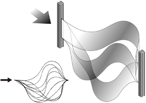
The snap-through (snapping) motion, in which a system undergoes a rapid transition from one equilibrium state to another, has attracted attention because of its novel dynamic characteristics. In such motion, the energy stored in a structure is suddenly converted to kinetic energy when the system begins to snap, inducing a rapid movement of the structure until it reaches the other equilibrium. Several instances of snap-through motion are found in nature and everyday life, such as the Venus flytrap (Forterre et al. Reference Forterre, Skotheim, Dumais and Mahadevan2005; Poppinga & Joyeux Reference Poppinga and Joyeux2011), hopper poppers (Pandey et al. Reference Pandey, Moulton, Vella and Holmes2014) and hairpins. The snap-through motion of elastic materials has also been investigated with medical and engineering applications in mind, i.e. ventricular assist devices (Gonçalves et al. Reference Gonçalves, Pamplona, Teixeira, Jerusalmi, Cestari and Leirner2003), actuators such as on/off switches (Han, Ko & Korvink Reference Han, Ko and Korvink2004), high-speed transport systems for hydrogels (Xia, Lee & Fang Reference Xia, Lee and Fang2010), flow regulators (Arena et al. Reference Arena, Groh, Brinkmeyer, Theunissen, Weaver and Pirrera2017) and energy harvesters using electrostatic or piezoelectric transducers (Boisseau et al. Reference Boisseau, Despesse, Monfray, Puscasu and Skotnicki2013; Zhu & Zu Reference Zhu and Zu2013).
External energy input can initiate a rapid snapping transition. In previous studies, snapping was achieved by imposing local mechanical inputs such as a point load or a moment at a point on a buckled structure (Chen & Hung Reference Chen and Hung2011; Pandey et al. Reference Pandey, Moulton, Vella and Holmes2014; Cleary & Su Reference Cleary and Su2015) and a torque that controls the inclination angle of two clamped edges (Beharic, Lucas & Harnett Reference Beharic, Lucas and Harnett2014; Gomez, Moulton & Vella Reference Gomez, Moulton and Vella2017a). Snapping can also occur through the application of distributed external inputs such as electrostatic loading (Krylov, Ilic & Lulinsky Reference Krylov, Ilic and Lulinsky2011), photomechanical effects (Shankar et al. Reference Shankar, Smith, Tondiglia, Lee, McConney, Wang, Tan and White2013) and thermal effects (Boisseau et al. Reference Boisseau, Despesse, Monfray, Puscasu and Skotnicki2013). Regarding a fluid-induced mechanism, Fargette, Neukirch & Antkowiak (Reference Fargette, Neukirch and Antkowiak2014) deposited a single droplet locally on an elastic sheet to induce snap-through. Snap-through arises when the sheet, which has maintained the balance among the capillary force of the droplet, the gravitational force of the droplet and the bending force of the sheet, loses its equilibrium. For example, when the droplet is deposited on the lower surface of a downward buckled sheet and the volume of the droplet reaches a critical value, the capillary force overcomes the sum of the gravitational force and the bending force, and the sheet snaps to an upward buckled state.
In addition to the aforementioned external triggers, a few studies have considered fluid flow as a mechanism for realizing the snap-through of a buckled sheet. Arena et al. (Reference Arena, Groh, Brinkmeyer, Theunissen, Weaver and Pirrera2017) suggested the conceptual design of a shape-adaptive air inlet using a buckled sheet for application to flow regulating systems. By properly adjusting the boundary conditions, such as angles and the transverse positions of clamped ends, snap-through and snap-back of a sheet could be controlled to open and close the air inlet. Gomez, Moulton & Vella (Reference Gomez, Moulton and Vella2017b) explored the one-off snap-through of a sheet by fluid-dynamic loading in a small-scale flow channel with cross-sectional dimensions of the order of a centimetre at Reynolds number  ${Re} = O(10^{-2})$. To predict the deformed shape of the sheet at each equilibrium state for a given fluid flux, they coupled the linearized Euler–Bernoulli beam equation with the fluid pressure distribution modelled using the lubrication theory and Poiseuille's law. Furthermore, Peretz et al. (Reference Peretz, Mishra, Shepherd and Gat2020) introduced a continuous multistable structure with a slender elastic membrane. By imposing arbitrary time-dependent pressure profiles at an inlet, actuating fluid could induce either snap-up or snap-down of the membrane and produce various deformation patterns with multiple transition regions between snap-up and snap-down along the membrane. Kim et al. (Reference Kim, Zhou, Kim and Oh2020) recently proposed a snap-through-based triboelectric energy harvesting system operating in unbounded flow. A buckled sheet was found to experience periodic snapping oscillations when it was exposed to an external uniform wind, and electrical energy was extracted from periodic contact between the snapping sheet and the sidewalls. Although the flow-induced snap-through mechanism at high Reynolds numbers was explored by Kim et al. (Reference Kim, Zhou, Kim and Oh2020), the fluid-mechanical principles of the transition to periodic oscillation remain unclear.
To understand the interaction of an elastic sheet with unbounded uniform flow, it is important to establish a proper fluid force model acting on the sheet, which should be coupled with the governing equation of the sheet. When the Reynolds number of the flow is sufficiently large, the fluid force by viscous effects is negligible compared with the normal force due to the pressure difference between the two sides of the sheet. Alben, Shelley & Zhang (Reference Alben, Shelley and Zhang2002) assumed that fluid pressure behind the location on the fibre where flow separation occurs was equal to a constant wake pressure, which was based on the free-streamline theory, and determined the pressure jump between the two sides of the deflected fibre at equilibrium, using the steady Bernoulli equation and setting the wake pressure as zero. Regarding problems where a thin structure is at equilibrium or has a much slower velocity in deformation compared with the flow speed, quasi-steady flow force models have been applied for the pressure jump across the structure. Examples of the problems include the reconfiguration of a sheet clamped at a certain angle to the flow direction (Gosselin, de Langre & Machado-Almeida Reference Gosselin, de Langre and Machado-Almeida2010; Luhar & Nepf Reference Luhar and Nepf2011), the dynamics of clapping papers in a book (Buchak, Eloy & Reis Reference Buchak, Eloy and Reis2010) and the stability of an inverted flag (Sader et al. Reference Sader, Cossé, Kim, Fan and Gharib2016a; Sader, Huertas-Cerdeira & Gharib Reference Sader, Huertas-Cerdeira and Gharib2016b; Tavallaeinejad, Païdoussis & Legrand Reference Tavallaeinejad, Païdoussis and Legrand2018). In addition, unsteady fluid force models have been employed, such as the unsteady Bernoulli equation to predict the critical velocity and post-critical dynamics for flag flutter (Guo & Païdoussis Reference Guo and Païdoussis2000; Eloy, Souilliez & Schouveiler Reference Eloy, Souilliez and Schouveiler2007; Jia et al. Reference Jia, Li, Yin and Yin2007; Eloy et al. Reference Eloy, Lagrange, Souilliez and Schouveiler2008; Alben Reference Alben2009) and the inviscid vortex model to examine the correlation between the nonlinear dynamics and wake patterns of a flag (Tang & Païdoussis Reference Tang and Païdoussis2007; Alben & Shelley Reference Alben and Shelley2008; Michelin, Llewellyn Smith & Glover Reference Michelin, Llewellyn Smith and Glover2008).
Generally, an elastic sheet parallel to either unbounded or bounded flow undergoes a transition from a static equilibrium to limit-cycle oscillations, and the critical conditions for the transition depend on the model configurations. For a flag whose trailing edge is free to move, a resonant bending instability caused by a non-uniform pressure distribution is responsible for the transition to fluttering motion (Guo & Païdoussis Reference Guo and Païdoussis2000; Argentina & Mahadevan Reference Argentina and Mahadevan2005; Eloy et al. Reference Eloy, Souilliez and Schouveiler2007). For the critical conditions of such flutter instability, the mass ratio, which represents the relative magnitude of fluid inertia to solid inertia, has been considered as an important parameter in addition to the dimensionless free-stream velocity, defined as the ratio of fluid inertial force to bending force, and the aspect ratio, defined as the ratio of height to length of the sheet. In contrast, for an inverted flag with a free leading edge and a clamped trailing edge, the effect of the mass ratio on the critical velocity was found to be negligible, following divergence instability (Kim et al. Reference Kim, Cossé, Cerdeira and Gharib2013; Sader et al. Reference Sader, Cossé, Kim, Fan and Gharib2016a; Kim & Kim Reference Kim and Kim2019). While periodic wave patterns develop along a structure and the effects of unsteady fluid forces are of importance in a transition by the flutter instability, the divergence instability is a static rather than a dynamic form of instability, and it can be determined by neglecting the inertial effects of the structure (Païdoussis, Price & de Langre Reference Païdoussis, Price and de Langre2010). In the divergence instability, the structure begins to deform monotonically on one side from its static equilibrium shape at the critical condition.
On the other hand, for an extensible flat membrane embedded in a channel, the effects of the Reynolds number and tension applied to the membrane on the membrane deformation have been investigated (Jensen & Heil Reference Jensen and Heil2003; Inamdar, Wang & Christov Reference Inamdar, Wang and Christov2020). Jensen & Heil (Reference Jensen and Heil2003) theoretically obtained the critical condition for the onset of self-excited oscillations in terms of the Reynolds number and reported that the critical Reynolds number strongly depended on the tension on the membrane and the length of the rigid parts located at the front and back of the membrane. For an inextensible post-buckled sheet in a channel flow at a much lower Reynolds number than the aforementioned studies, Gomez et al. (Reference Gomez, Moulton and Vella2017b) found that the critical fluid flux through the channel to initiate snap-through depended on a channel-blocking parameter, which is determined by the compression ratio of the sheet.
Motivated by potential fluid energy harvesting applications using piezoelectric and triboelectric materials, this study investigates the stability and nonlinear snap-through dynamics of an initially buckled elastic sheet under an unbounded external flow with  ${Re} = O(10^{4}\text {--}10^{5})$. The deformed shapes in the equilibrium states and the critical velocity for the onset of snapping are obtained experimentally by changing certain geometric and dynamic parameters, such as the initial buckled shape, free-stream velocity and fluid density. Experimental measurements are then compared with the predictions given by low-order numerical simulations, which employ the elastica model for the sheet deformation and the quasi-steady fluid force model based on Bollay's lift theory. Our experimental set-up is described in § 2. The theoretical approach and numerical method for an equilibrium state are presented in §§ 3.1 and 3.2, respectively. The behaviour of the sheet at the equilibrium state is analysed using the results of experimental measurements and numerical simulations in § 3.3, which is followed by discussion on the critical condition of the sheet in § 4. We also examine the nonlinear responses of periodic oscillations in a post-equilibrium state in terms of the oscillation frequency (§ 5.1), modal shape (§ 5.2) and elastic bending energy (§ 5.3). Finally, the key findings of this study are summarized in § 6.
2. Experimental set-up
An open-loop wind tunnel with a cross-section of height  $60$ cm and width
  $60$ cm generates a free stream with spatial uniformity of within 2 %. The free-stream velocity ranges from
  $0.1$ to
  $13.0$ m s
 $^{-1}$. Both ends of a polycarbonate sheet (density
  $\rho _s = 1200$ kg m
 $^{-3}$ and elastic modulus
  $E = 2.38\times 10^{9}$ N m
 $^{-2}$) of length
  $L = 32.5$–60.0 cm, height
  $H = 5.0$–7.5 cm and thickness
  $h = 0.20$–0.38 mm are clamped parallel to the free stream by vertical aluminium poles; the distance between the poles is
  $L_0 = 30$–40 cm (figure 1), and both poles are on the
  $y = 0$ line, with no transverse deviation between them (see inset of figure 1). For the initial buckling,
  $L_0$ is adjusted to be less than
  $L$.
$L$.

Figure 1. Schematic diagram of the snap-through model. Inset: definition of coordinates.
Three dimensionless parameters that are of interest in characterizing the snap-through motion are the length ratio  $L^{*}$, aspect ratio
  $H^{*}$ and mass ratio
  $m^{*}$:
 \begin{equation} L^{*} = L_0/L, \quad H^{*} = H/L, \quad m^{*} =\rho_s h/\rho_f L, \end{equation}
where  $\rho _f$ is the fluid density. A sheet with a small length ratio exhibits large deflection, and a length ratio equal to unity represents a straight sheet. The sheet used in this study satisfies
  $h \ll H \ll L$ so that the sheet behaves as a thin strip in terms of its elasticity and has a high rigidity to out-of-plane deformation. Under this condition,
  $B =Eh^{3}/12$, which omits the Poisson ratio, can be used as the bending stiffness of the sheet per unit height (Audoly & Pomeau Reference Audoly and Pomeau2010). In addition to
  $h \ll L$, the dimensionless end-shortening
  $1-L^{*}\ (=(L-L_0)/L)$ is much greater than the stretchability
  $S\ (= h^{2}/(12L^{2}))$ in our model:
  $(1-L^{*})/S>10^{6}$. Thus, the extensibility of the sheet is negligible (Pandey et al. Reference Pandey, Moulton, Vella and Holmes2014). An appropriate choice of the bending stiffness
  $B$ and sheet geometry enables us to achieve two-dimensional horizontal motion while avoiding three-dimensional motion along the vertical direction and sagging due to gravity. Because the motion is restricted to two dimensions, filming the bottom edge of the sheet using a high-speed camera (FASTCAM MINI UX50, Photron Inc.) is sufficient for measuring the sheet deformation. Images of the sheets were captured at
  $125$ frames per second with a shutter speed of
  $1/2000$ s and processed with MATLAB (Mathworks Inc.) to track the positions of the sheets.
Additional experimental measurements were conducted in a water tunnel of width  $0.5$ m, length
  $1.2$ m and free-surface height
  $0.4$ m in order to investigate the effect of the mass ratio on the critical velocity. The free-stream velocity ranges from
  $0.1$ to
  $0.5$ m s
 $^{-1}$, and the overall experimental set-up is similar to that used in the wind tunnel experiments. A polycarbonate sheet of length
  $L = 35.0\text {--}60.0$ cm, height
  $H = 5$ cm and thickness
  $h = 0.38$ mm was used;
  $L_0 = 30.0\text {--}40.0$ cm.
For particle image velocimetry in the water tunnel, we reduced both  $L$ and
  $L_0$ to map a sufficient fluid domain around the sheet:
  $L = 26.7$ cm and
  $L_0 = 20.0$ cm (
 $L^{*} = 0.75$). Seeding particles with a mean diameter of
  $50\ \mathrm {\mu }$m were illuminated by a pulsed Nd:YAG laser sheet (Evergreen200, Quantel Inc.) on the mid-height of the sheet. Two identical cameras (GEV-B1620M, Im-perx Inc.) were mounted below the bottom section of the water tunnel. The two images captured simultaneously by the two cameras were merged into one image using MATLAB. Image pairs were captured every
  $0.033$ s, and the time delay between a pair of images was
  $0.006$ s. PIVview2C (version 3.6.0, PIVTEC GmbH) was used to cross-correlate the image pairs. For the multi-grid interrogation method, the initial sample window was 96 pixels
  $\times$ 96 pixels and the final window size was 24 pixels
  $\times$ 24 pixels, producing
  $94 \times 65$ nodes in a single velocity field.
3. Equilibrium state prior to snap-through
A buckled sheet with no fluid flow initially exhibits fore–aft symmetry and becomes deformed along the flow direction with increasing free-stream velocity. The deformed sheet maintains an equilibrium state at each free-stream velocity. When the velocity reaches a critical value, the sheet begins to snap quickly to the opposite side. In this section, the deformed shape of the buckled sheet is examined in the equilibrium state prior to snap-through. Although some minor fluctuations are observed in the deformed sheet exposed to fluid loading, its magnitude is sufficiently small that the equilibrium state is assumed before the bifurcation occurs.
3.1. Problem description
3.1.1. Initial equilibrium state without flow
In the absence of fluid flow, a differential equation describing the buckled sheet can be written in terms of the local balance of moments:
 \begin{equation} B\frac{{\textrm{d}}^{2}\theta(s)}{{\textrm{d}}s^{2}}+P_0\sin\theta(s)=0,\end{equation}
where  $s$ is the curvilinear coordinate,
  $\theta$ is the angle between the sheet and the
  $x$-axis (inset of figure 1) and
  $P_0$ is the compressive reaction force per unit height applied at the front end (
 $s = 0$) of the sheet in the positive
  $x$-direction. Note that
  $P_0$ is also applied at the rear end (
 $s = L$) of the sheet in the negative
  $x$-direction.
Because the sheet is clamped at both edges, Dirichlet boundary conditions are applied at both edges:  $\theta (s=0) = \theta (s=L) = 0$. Moreover, for the fundamental buckling mode with the fore–aft symmetric shape and the two clamped ends on the same
  $y = 0$ line, the
  $y$-directional reaction force
  $F_y$ at both ends is zero. If a deviation in the
  $y$-direction exists between the positions of the two clamped ends or an asymmetric buckling mode of a higher order is considered as an initial shape, an additional term with a non-zero
  $F_y$ at the front end should be involved in (3.1). Because a length ratio in the range
  $L^{*} = 0.5$–
 $0.9$ can cause large deflection, the nonlinear equation from the elastica theory is adopted instead of the linear equation (Timoshenko & Gere Reference Timoshenko and Gere2009). For a flapping flag model in which one edge is free to move, the relative importance of compressive force (tensile force) depends on the model conditions and flow regime (Shelley, Vandenberghe & Zhang Reference Shelley, Vandenberghe and Zhang2005), and the compressive force is generally neglected. However, for the buckled sheet model, the compressive force should be balanced by the bending force, even in the absence of fluid flow, to achieve the post-buckling configuration imposed by end-shortening (
 $L_0<L$).
The buckled sheet without fluid flow is in four-fold symmetry, provided that both ends are on the same  $y$-coordinate. The total shape of the sheet is composed of four identical pieces, and the total shape can be constructed by rotating and reflecting the pieces (Timoshenko & Gere Reference Timoshenko and Gere2009; Wagner & Vella Reference Wagner and Vella2013). Thus, we consider only a quarter of the sheet from
  $s=0$ to
  $s=L/4$ to solve (3.1). To obtain the shape of the sheet piece, the compressive force
  $P_0$ at
  $s = 0$ and the angle at the inflection point,
  $s = L/4$, with zero curvature value (
 ${\textrm {d}} \theta /{\textrm {d}}s = 0$) are first calculated for given
  $L$ and
  $L_0$ (and thus
  $L^{*}$), using elliptical integrals in (3.2a,b) (Timoshenko & Gere Reference Timoshenko and Gere2009):
 \begin{equation} \frac{1}{4}L_0=2\left(\frac{EI}{P_0}\right)^{{1}/{2}} \textrm{E}\left[\sin\frac{\theta_0}{2}\right]-\frac{1}{4}L \quad\textrm{and}\quad \frac{1}{4}L=4\left(\frac{EI}{P_0}\right)^{{1}/{2}} \textrm{K}\left[\sin\frac{\theta_0}{2}\right], \end{equation}
where  $\textrm {K}[~]$ and
  $\textrm {E}[~]$ are the complete elliptical integrals of the first and second kinds, respectively. The shape of the sheet piece is then obtained numerically by solving (3.1) with the
  $P_0$ value and boundary conditions,
  ${\textrm {d}} \theta /{\textrm {d}}s = 0$ and
  $\theta = \theta _0$ at the inflection point (
 $s = L/4$). Additionally, for given
  $L$ and
  $L_0$, the maximum transverse displacement
  $w_0$ of the total sheet, which appears at
  $s = L/2$, can be calculated from
 \begin{equation} \frac{1}{2}w_0=2\left(\frac{EI}{P_0}\right)^{{1}/{2}}\sin\frac{\theta_0}{2}. \end{equation}
The deformed shapes with no fluid flow, which are predicted by the nonlinear equation (3.1) and the linear Euler–Bernoulli equation, are compared in appendix A.
3.1.2. Equilibrium state with flow
On the other hand, with fluid flow, the fluid force  $F_f$ normal to the surface of the sheet is exerted on the buckled sheet as a distributed load, and the reaction force
  $F_y$ in the
  $y$-direction is additionally imposed at the front end (
 $s = 0$) of the sheet (figure 2a);
  $F_y$ is zero without the fluid force. The fluid force on the sheet with a finite aspect ratio can be modelled with the combination of resistive force and reactive force (Lighthill Reference Lighthill1960; Buchak et al. Reference Buchak, Eloy and Reis2010; Michelin & Doaré Reference Michelin and Doaré2013; Tavallaeinejad et al. Reference Tavallaeinejad, Païdoussis and Legrand2018). The resistive force is expressed as the normal force experienced by a flat plate under fluid flow, and the reactive force is caused by an acceleration of the fluid flow that follows the shape of the sheet. Because the deformed sheet maintains an equilibrium state at each free-stream velocity before the sheet begins to snap at a critical velocity, the quasi-steady fluid force is assumed. Moreover, for a slender sheet at the equilibrium state, the magnitude of the reactive force, which scales with the square of sheet height, is much smaller than that of the resistive force, which scales with the sheet height. In this study, we use slender sheets with small aspect ratios in
  $H^{*} = [0.07\text {--}0.18]$ and thus consider only the resistive fluid force for simplicity. To establish an equilibrium equation in terms of moment balance at a given coordinate
  $s$, we first divide the quasi-steady resistive fluid force
  $F_f$ into two components,
  $F_{f,x}$ and
  $F_{f,y}$. Then, the fluid force components per infinitesimal segment
  ${\textrm {d}}s$ and per unit height are modelled as
 \begin{equation} {\textrm{d}}F_{f,x} = \tfrac{1}{2}\rho_f U^{2} C_D(s)\, {\textrm{d}}s \quad\textrm{and}\quad {\textrm{d}}F_{f,y} = \tfrac{1}{2}\rho_f U^{2} C_L(s)\, {\textrm{d}}s. \end{equation}
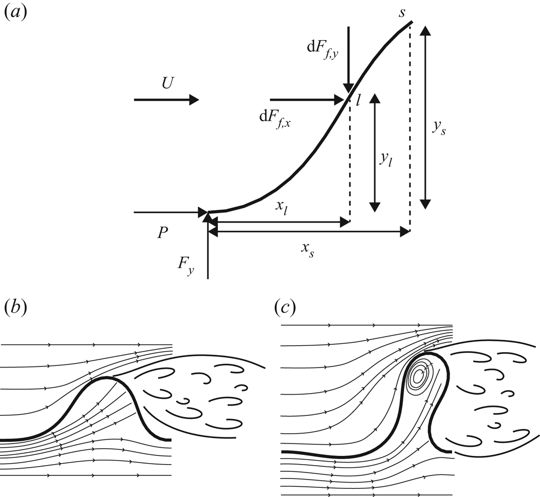
Figure 2. (a) Schematic diagram of the forces imposed on the sheet from the front end ( $s = 0$) to a given coordinate
  $s$. (b,c) Illustration of streamlines around the sheet for (b) a large length ratio (
 $L^{*} = 0.75$) and (c) a small length ratio (
 $L^{*} = 0.50$).
For the quasi-steady fluid force model, Bollay (Reference Bollay1939) presented the normal force coefficient of a rectangular wing with a small aspect ratio, which was established by a nonlinear wing theory. Because the normal force coefficient in Bollay (Reference Bollay1939) did not have an explicit form, Polhamus (Reference Polhamus1966) proposed the explicit form of the normal force acting on an inclined rigid plate with an angle of attack of  $\theta$, using leading-edge suction analogy. The normal coefficient
  $C_N$, drag coefficient
 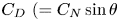 $C_D\ (= C_N\sin \theta$) and lift coefficient
  $C_L\ (= C_N\cos \theta$) are expressed as follows:
 \begin{gather} C_N(\theta) = K_p\sin\theta\cos\theta + K_v\sin^{2}\theta , \end{gather}
 \begin{gather}C_D(\theta) = K_p\sin^{2}\theta\cos\theta + K_v\sin^{3}\theta , \end{gather}
 \begin{gather}C_L(\theta) = K_p\sin\theta\cos^{2}\theta + K_v\sin^{2}\theta\cos\theta, \end{gather}
where  $K_p$ and
  $K_v$ in (3.5) are associated with potential lift and vortex lift, respectively, and they are functions of the aspect ratio
  $H^{*}$ of the sheet only. Tavallaeinejad et al. (Reference Tavallaeinejad, Païdoussis and Legrand2018) obtained fitting curves for
  $K_p$ and
  $K_v$ in a wide range of
  $H^{*}$ based on the results of Bollay (Reference Bollay1939). In the present study, the fitting curves presented in Tavallaeinejad et al. (Reference Tavallaeinejad, Païdoussis and Legrand2018) are used to extract
  $K_p$ and
  $K_v$ values for a given
  $H^{*}$. The viscous shear stress exerted on the sheet roughly scales as
  $\mu U/\delta$, where
  $\mu$ is the dynamic viscosity of the fluid and
  $\delta$ is the representative boundary layer thickness. As the Reynolds number
  ${Re}\ (=UL/\nu )$ is
  $O(10^{4}$–
 $10^{5})$ in this study, the boundary layer is laminar, and accordingly
  $\delta \sim {Re}^{-{1}/{2}}L$. The relative magnitude of the tangential force per unit area (viscous shear stress),
  $\mu U/\delta$, over the normal resistive force per unit area,
  $\frac {1}{2}\rho _f U^{2} C_N$, scales as
  ${Re}^{-{1}/{2}}/C_N$. Because
  ${Re} = O(10^{4}$–
 $10^{5})$ and
  $C_N = O(10^{0})$, the force induced by the viscous stress can be neglected.
Using  $F_{f,x}$,
  $F_{f,y}$ and the internal reaction forces (
 $P$ and
  $F_y$), the local balance of moments per unit length at
  $s$ is formulated as
 \begin{align} &B\frac{{\textrm{d}}^{2}\theta(s)}{{\textrm{d}}s^{2}}+\left[P+\frac{1}{2}\rho_fU^{2} \int_{0}^{s}{C_D(\theta(l))\, {\textrm{d}}l}\right]\sin\theta(s)\nonumber\\ &\quad -\left[F_y-\frac{1}{2}\rho_fU^{2}\int_{0}^{s}{C_L(\theta(l))\, {\textrm{d}}l}\right] \cos\theta(s)=0. \end{align}
Note that  $F_{f,y}$ is positive along the negative
  $y$-direction (figure 2a). By combining the two integrals in (3.6), one obtains
 \begin{align} B\frac{{\textrm{d}}^{2}\theta(s)}{{\textrm{d}}s^{2}}+P\sin\theta(s)-F_y\cos\theta(s)+ \frac{1}{2}\rho_fU^{2}\int_{0}^{s}{C_N(\theta(l))\cos(\theta(l)-\theta(s))\, {\textrm{d}}l}=0. \end{align}
The left-hand side of (3.7) indicates the local balance of moments, which is caused by the bending shear force, internal forces and normal component of fluid force. For the prediction of the stability boundary where the transition appears, the inertial force term of the sheet can be omitted from the equation; this approach will be justified in § 4, where the effect of the mass ratio on the transition is discussed.
Equation (3.7) is only applicable for  $0\leq s < s|_{y = y_{max}}$, because the free stream does not directly impose any force on the sheet for
  $s \geq s|_{y=y_{max}}$;
  $s|_{y=y_{max}}$ is the apex of the sheet (the point of maximum transverse displacement). As for the outer (positive
  $y$) side of the sheet, if the flow separation occurs at the apex of the sheet, the pressure on the outer side behind the apex can be roughly approximated to be constant because of the formation of the wake (figure 2b,c) (Alben et al. Reference Alben, Shelley and Zhang2002). For the sheet with a small aspect ratio
  $H^{*} = [0.07\text {--}0.18]$ considered in our study, the free stream is entrained into the area below the buckled sheet, and the entrained flow can exert a loading on the rear part of the sheet.
The pressure difference between the two surfaces of the rear part depends on the  $L^{*}$ value, which determines the volume of space below the buckled part. For
  $L^{*}$ close to unity (small initial deflection), because of a small change in the direction for the entrained flow (figure 2b), the entrained flow can exert a great loading on the rear part of the sheet. The pressure difference between the two surfaces of the rear part is not negligible, and thus it should be considered to precisely predict the deformed shape. However, instead of the complicated modelling of the pressure difference for
  $L^{*}$ close to unity, we roughly assume that the effect of pressure difference in the rear part is relatively small and no net fluid-dynamic loading is applied on the rear part because the pressure difference in the front part is more critical to determine the overall shape of the sheet. In § 3.3, we will report that, despite this rough assumption, numerical simulation results for the deformed shape are in good agreement with experimental results for
  $L^{*}$ close to unity. On the other hand, for a small
  $L^{*}$ with large initial deflection, the entrained flow inside the buckled part veers greatly, as shown in figure 2(c), forming a circulating region, which eventually results in negligible pressure difference between the two surfaces on the rear part.
In summary, for all  $L^{*}$ addressed in this study, we assume that no net fluid-dynamic loading is applied on the rear part, and the following two equations, (3.8a) and (3.8b), are used to predict the equilibrium shape of the sheet at each free-stream velocity before bifurcation and to find the critical velocity:
 \begin{align} &B\frac{{\textrm{d}}^{2}\theta(s)}{{\textrm{d}}s^{2}}+P\sin\theta(s)-F_y\cos\theta(s)\nonumber\\ &\quad +\frac{1}{2}\rho_fU^{2}\int_{0}^{s}{C_N(\theta(l))\cos(\theta(l) -\theta(s))\, {\textrm{d}}l}=0, \quad s < s|_{y = y_{max}},\end{align}
 \begin{align} &B\frac{{\textrm{d}}^{2}\theta(s)}{{\textrm{d}}s^{2}}+P\sin\theta(s)-F_y\cos\theta(s)\nonumber\\ &\quad +\frac{1}{2}\rho_fU^{2}\int_{0}^{s_{y_{max}}}{C_N(\theta(l))\cos(\theta(l) -\theta(s))\, {\textrm{d}}l}=0, \quad s \geq s|_{y = y_{max}}. \end{align}
The governing equations differ between the regions before and after the apex.
3.2. Numerical method
To solve nonlinear equations (3.8a) and (3.8b), numerical simulations are required. The solution of (3.1) corresponding to  $U = 0$ is used as an initial guess for the given model. For the finite-difference method, the sheet is discretized into segments of constant length
  ${\rm \Delta} s = L/N$, where
  $N$ is the number of grids (
 $N = 61$). The discretized forms of (3.8a) and (3.8b) at each grid point
  $i$ are
 \begin{align} &B\frac{\theta_{i+1}-2\theta_i+\theta_{i-1}}{({\rm \Delta} s)^{2}} +\left[P+\frac{1}{2}\rho_fU^{2}\int_{0}^{s_i}{C_D(\theta(l))\, {\textrm{d}}l}\right]\sin\theta_i \nonumber\\ &\quad -\left[F_y-\frac{1}{2}\rho_fU^{2}\int_{0}^{s_i}{C_L(\theta(l))\, {\textrm{d}}l}\right] \cos\theta_i=0, \quad i = 1,\ldots,m, \end{align}
 \begin{align} &B\frac{\theta_{i+1}-2\theta_i+\theta_{i-1}}{({\rm \Delta} s)^{2}}+ \left[P+\frac{1}{2}\rho_fU^{2}\int_{0}^{s_m}{C_D(\theta(l))\, {\textrm{d}}l}\right]\sin\theta_i \nonumber\\ &\quad -\left[F_y-\frac{1}{2}\rho_fU^{2}\int_{0}^{s_m}{C_L(\theta(l))\, {\textrm{d}}l}\right] \cos\theta_i=0,\quad i = m+1,\ldots,N-1, \end{align}
where  $\theta _i = \theta (i{\rm \Delta} s)$,
  ${\textrm {d}}^{2}\theta /{\textrm {d}}s^{2}$ is discretized using the standard second-order difference method and
  $m$ is the grid point immediately before
  $s|_{y=y_{max}}$. The integrals in (3.9a) and (3.9b) are evaluated with the extended trapezoidal rule. Starting from the initial solution for
  $U = 0$, the solution at each
  $U$ is obtained with intervals of
  ${\rm \Delta} U$ varying from 0.50 at low
  $U$ to 0.05 near
  $U = U_c$. The
  $\theta$ values of the previous step are used to compute
  $C_D$ and
  $C_L$ in the current step, and
  $s|_{y=y_{max}}$ from the previous step is used to determine which of (3.9a) and (3.9b) is used for each grid point. Because the sheet is clamped at both edges, boundary conditions are applied as
 \begin{equation} \theta_{{front} (i=1)} = \theta_{{rear} (i=N)}=0.\end{equation}
 Equations (3.9a) and (3.9b) with (3.10) form a system of nonlinear equations that can be solved using Newton's method at each  $U$. The
  $P$ and
  $F_y$ values are adjusted by the shooting method until the solution satisfies the following boundary conditions at the rear end:
  $x(L) = L_0$ and
  $y(L) = 0$. Iteration ceases when the total error at the rear end is
  $\epsilon = (\epsilon _x^{2} + \epsilon _y^{2})^{{1}/{2}} \leq L \times 10^{-4}$, where
  $\epsilon _x = |x_N - L_0|$ and
  $\epsilon _y = |y_N - 0|$. According to our numerical simulation, when
  $U$ reaches a certain velocity, there exists no solution that satisfies the error criterion at the rear end, which means that the equilibrium state is no longer possible. That velocity is defined as the critical flow velocity, beyond which an inertial effect of the sheet should be considered. The critical flow velocity and transition to limit-cycle oscillation are discussed in § 4. We also conducted two separate convergence tests with a smaller
  ${\rm \Delta} U$ and a larger
  $N$. For
  $L^{*} = 0.50$ and
  $0.86$, the differences in the shape deformation at each
  $U$ and the critical velocity were found to be negligible between the original result and the new result using the smaller
  ${\rm \Delta} U$ varying from
  $0.10$ at low
  $U$ to
  $0.025$ near
  $U = U_c$. Furthermore, the difference in the equilibrium shapes at each
  $U$ between the two cases using 61 and 201 grid points was negligible. For example, near
  $U = U_c$, the maximum difference in the
  $y$-coordinate between the two cases,
  $({\rm \Delta} y)_{max}/L_0$, was just
  $0.003$ at
  $L^{*} = 0.50$.
3.3. Shape of a sheet at equilibrium
For an equilibrium shape at each free-stream velocity and length ratio before bifurcation, the numerical solution of (3.9) and (3.10) is in excellent agreement with the experimental result, despite the simple modelling of the fluid force (figure 3a). Depending on the length ratio  $L^{*}$, the sheets show different trends in deformation. For a large
  $L^{*}$ close to unity (smaller deflection), the apex of the sheet is mainly displaced in the streamwise direction as
  $U$ increases, and the transverse location of the apex remains similar (figure 3ai), which leads to an enhanced curvature at the rear part of the sheet. Until the free-stream velocity reaches the critical velocity, the streamwise shift of the apex is primarily observed, and the sheet does not cross the midline (straight line between the two clamped ends).

Figure 3. (a) Superimposed equilibrium shapes of the buckled sheet for several free-stream velocities before bifurcation:  $[L^{*}, H^{*}, m^{*}] = [0.86, 0.14, 1.09]$ (i);
  $[0.75, 0.13, 0.95]$ (ii);
  $[0.60, 0.10, 0.76]$ (iii); and
  $[0.43, 0.07, 0.54]$ (iv). The black solid lines are obtained by our experimental measurements, and the red dotted lines are from our numerical simulations. (b,c) The
  $y$-coordinate (
 $y/w_0$) of the sheet at
  $x = L_0/2$ versus
  $U^{*}$ from (b) the numerical simulations and (c) the experimental measurements:
  $H^{*} = [0.08\text {--}0.14]$. In panels (b) and (c), the colour of the dot denotes the magnitude of
  $L^{*}\ (=0.50\text {--}0.86)$ as in the colour bar: the same colour for a given
  $L^{*}$. Each dot represents the case of a specific
  $U^{*}$ increasing from
  $U^{*} = 0$.
For a small  $L^{*}$, the front part of the sheet undergoes significant streamwise movement as well as transverse movement as
  $U$ increases, and the front part can cross the midline when
  $U$ is close to the critical velocity (figure 3aii,aiii). For a smaller
  $L^{*}$, the buckled sheet continues to deform along the flow direction on one side (figure 3aiv). In this case, as the flow velocity increases, the part near the apex of the sheet bends backwards. Subsequently, two points of the sheet can contact each other to form a teardrop shape, and the snap-through does not appear, even for a higher
  $U$. This state cannot be obtained by the numerical simulations; in figure 3(aiv), the red dotted line corresponding to the numerical simulation is not provided for the most deformed shape.
The deformation of our snap-through model can be compared with that of another snap-through model under fluid flow studied by Gomez et al. (Reference Gomez, Moulton and Vella2017b). The deformations of both models are similar in that, for a smaller  $L^{*}$, the displacement of the sheet becomes more notable with increasing flow velocity. However, the detailed deformed configurations vary slightly because a different type of fluid flow and different range of the length ratio were used in Gomez et al. (Reference Gomez, Moulton and Vella2017b). The range of the length ratio in Gomez et al. (Reference Gomez, Moulton and Vella2017b) is much closer to unity (
 $L^{*} > 0.96$) than that of our model, and thus, for each point on the sheet, the transverse displacement is dominant over the streamwise displacement. Because the model of Gomez et al. (Reference Gomez, Moulton and Vella2017b) is confined in a narrow flow channel with strong blockage effect at
  ${Re} = O(10^{-2})$, hydrodynamic pressure on the buckled sheet decreases monotonically along the streamwise direction, indicating that a large fluid loading is imposed on the front part of the sheet. Accordingly, the front part of the sheet can cross the midline even for
  $L^{*} > 0.96$; see supplementary figure 3 in Gomez et al. (Reference Gomez, Moulton and Vella2017b). On the other hand, because the initial deflection of our model is greater than that of Gomez et al. (Reference Gomez, Moulton and Vella2017b), both streamwise and transverse displacements are important in our model, in particular for a small
  $L^{*}$ (figure 3a). Moreover, for our model in unbounded flow, the fluid force (3.4a,b) is affected solely by the deflection angle
  $\theta$ at each point on the sheet, in contrast to the model confined in a narrow channel. For
  $L^{*}$ close to unity, because of a small deflection angle, the fluid force imposed on the front part of the sheet along the transverse direction is small, and the sheet does not cross the midline before snap-through instability occurs.
To quantitatively investigate the deformation of a sheet at the equilibrium state, we introduce a dimensionless free-stream velocity  $U^{*}$ suitable for the snap-through model and use it instead of
  $U$ hereafter. The fluid inertial force exerted on the sheet per unit height scales simply as
  $F_f \sim \rho _f U^{2}w_0$, where
  $w_0$ indicates the maximum transverse displacement of the sheet in the absence of fluid flow: the frontal area of the sheet at
  $U = 0$ (figure 1). The bending force per unit height scales as
  $F_b \sim B/L^{2}$. Then, the dimensionless free-stream velocity, which represents the ratio of the fluid inertial force to the bending force, is defined as
  $U^{*} = U(\rho _fw_0L^{2}/B)^{{1}/{2}}$. As the definition of
  $U^{*}$ in this study includes
  $w_0$, it differs from the form generally used for flapping flag models,
  $U^{*}= U(\rho _f L^{3}/B)^{{1}/{2}}$ (e.g. Connell & Yue Reference Connell and Yue2007; Alben & Shelley Reference Alben and Shelley2008; Kim et al. Reference Kim, Cossé, Cerdeira and Gharib2013; Kim & Kim Reference Kim and Kim2019). For the flag models, the sheet length
  $L$ is the only length parameter to represent the geometrical feature of its two-dimensional profile. In contrast to the flag models, two length parameters,
  $L$ and
  $w_0$, are required together to represent the configuration of the buckled sheet. Thus, for the snap-through model,
 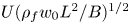 $U(\rho _fw_0L^{2}/B)^{{1}/{2}}$ is a more appropriate dimensionless velocity parameter to indicate the relative magnitude of the fluid inertial force and the bending force.
The deformation of the buckled sheet can be characterized by the transverse displacement  $y/w_0$ of the sheet at
  $x = L_0/2$. The transverse displacements acquired from numerical simulations are plotted as a function of the dimensionless free-stream velocity
  $U^{*}$ in figure 3(b). The
  $y/w_0$ values tend to collapse onto a single curve, regardless of the
  $L^{*}$ values considered in this study. While the variation in
  $y/w_0$ is minor in the low-
 $U^{*}$ regime,
  $y/w_0$ drops sharply in the high-
 $U^{*}$ regime. However, for a small
  $L^{*}$, the deformation of the sheet becomes more significant near the critical velocity, and accordingly the
  $y_{x=L_0/2}/w_0$ values of the sheet near the critical velocity tend to deviate from the collapsed curve (rightmost dots in figure 3b). Experimental results for
  $y_{x=L_0/2}/w_0$ also show a similar trend to the results of the numerical simulations despite some deviations (figure 3c).
Generally, snap-through instability follows a saddle-node bifurcation where the stable equilibrium and unstable equilibrium are closer with increasing bifurcation parameter such as flow rate or inclined angle at the clamped ends, and the two equilibrium states encounter each other at a critical value in a vertical fold (Gomez et al. Reference Gomez, Moulton and Vella2017a,Reference Gomez, Moulton and Vellab). The snap-through instability of our model using  $U^{*}$ as a bifurcation parameter seems to follow the saddle-node bifurcation, as can be inferred from figure 3(b,c). However, in figure 3(b,c), the
  $y_{x = L_0/2}/w_0$ values of all cases do not end at exactly vertical fold points. Even from our numerical simulation using a smaller step size of
  $U$ to examine the convergence of the results, the branches did not become more vertical at the critical velocity. The sheet could snap prematurely due to the presence of disturbance by the experimental set-up, and thus the vertical fold points may not be distinct, in contrast to the ideal saddle-node bifurcation diagram. In addition, our model may not exhibit a clear vertical fold due to the large deflection and streamwise shift of the sheet. More detailed theoretical examination on the bifurcation remains as a future study.
Moreover, the magnitudes of the two internal forces at the front end, the streamwise compressive force  $P$ and the transverse supporting force
  $F_y$ depicted in figure 2(a), are strongly affected by the free-stream velocity
  $U^{*}$ (and consequently by the change in the deformed shape) for each
  $L^{*}$. Notably,
  $P$ and
  $F_y$ exhibit opposite trends in terms of
  $U^{*}$ (figure 4a,b). In figure 4(a,b),
  $P$ and
  $F_y$ are normalized by the compressive force
  $P_0$ in the absence of fluid flow;
  $P/P_0 = 1$ at
  $U^{*} = 0$ for all cases of
  $L^{*}$. See appendix A for a detailed explanation of
  $P_0$. Without fluid flow, the compressive force at the front end of the sheet is positive, which means that it acts along the positive
  $x$-axis to maintain the bucked shape. As
  $U^{*}$ increases, the compressive force tends to decrease to maintain the force balance with the external fluid force acting along the positive
  $x$-axis (figure 4a). In particular, for
  $L^{*} = 0.50$ and
  $0.55$,
  $P/P_0$ becomes negative for large values of
  $U^{*}$. This indicates that, for a sheet with large initial deflection at high
  $U^{*}$, the fluid-dynamic loading distributed on the sheet along the streamwise direction is so large that the reaction force on the front end of the sheet should be negative for force balance; i.e. a tension force along the negative
  $x$-axis should be applied at the clamped end to maintain the given
  $L^{*}$.

Figure 4. (a) Dimensionless streamwise compressive force  $P/P_0$ and (b) transverse supporting force
  $F_y/P_0$ at the front end of the sheet for
  $L^{*} = 0.50$–
 $0.86$. The colour of the dot denotes the magnitude of
  $L^{*}$, as in the colour bar: the same colour for a given
  $L^{*}$. Each dot represents the case of a specific
  $U^{*}$ increasing from
  $U^{*} = 0$. The data in the two panels are from the numerical simulations with aspect ratio
  $H^{*} = [0.08\text {--}0.14]$. (c) Comparison of sheet deformations with increasing
  $U^{*}$ near
  $U_c^{*}$ between (i)
  $L^{*} = 0.86$ and (ii)
  $L^{*} = 0.50$.
Unlike  $P/P_0$, the supporting force
  $F_y/P_0$ tends to increase monotonically with
  $U^{*}$, although its slope varies with
  $L^{*}$ (figure 4b). Notably, the sheet with a small
  $L^{*}$ exhibits a sudden jump of
  $F_y$ near the critical velocity, which is attributed to the change in a deformation trend. As
  $U^{*}$ increases, the sheet with a large
  $L^{*}$ (
 $L^{*} = 0.86$ in figure 4c) gradually deforms without any sudden change in the deformation trend even near the critical velocity. However, for a small
  $L^{*}$ (
 $L^{*} = 0.50$ in figure 4c), the transverse displacement becomes dominant with increasing free-stream velocity, and the front part of the sheet crosses the midline (
 $y = 0$ line) after a certain free-stream velocity even in the equilibrium state. This notable transverse displacement of the sheet at a high free-stream velocity close to the critical velocity leads to the sudden jump of
  $F_y/P_0$ in figure 4(b).
4. Transition state
When the free-stream velocity reaches a critical value, the sheet begins to snap quickly to the opposite side, which is followed by periodic snap-through oscillations. During a half-cycle of the oscillation, two successive processes are observed: snapping to the opposite side and subsequent immediate shift along the streamwise direction (figure 5a). The sheet then repeats these processes to produce periodic oscillations; see the supplementary movie available at https://doi.org/10.1017/jfm.2021.57. Note that the numerical approach used in § 3 for the equilibrium state is not applicable to the transition and limit-cycle oscillations, and figure 5(a) is from experimental measurements.

Figure 5. (a) Superimposed sequential images of the sheet in the transition state, for  $[L^{*}, H^{*}, m^{*}, U^{*}] = [0.75, 0.13, 0.95, 11.10]$; only a half-cycle is presented. See the supplementary movie for periodic oscillations. (b) Critical flow velocity
  $U_c^{*}$ for snap-through transition. The sheet thickness is
  $h=0.20$ mm (red triangles),
  $0.25$ mm (blue stars),
  $0.30$ mm (magenta circles) and
  $0.38$ mm (green diamonds) for the experimental results. The results of numerical simulations using (3.9) (black asterisks) and scaling analysis (4.4) (black curve) are also shown. For the black curve,
  $U_c^{*} = 17.0[L^{*}(1-L^{*})]^{{1}/{4}}$. The discrepancy between (4.4) and experimental measurements increases as
  $L^{*}$ becomes smaller, which is denoted with the black dashed line. For the numerical data,
  $[L^{*}, H^{*}, m^{*}] = [0.50\text {--}0.86, 0.08\text {--}0.14, 0.63\text {--}1.08]$.
By varying the geometrical parameters of the sheet, critical flow velocities  $U_c^{*}$ for the onset of transition can be obtained experimentally (figure 5b). Interestingly, for all experimental cases,
  $U_c^{*}$ seemingly collapses onto a single curve, and its magnitude is governed by the length ratio
  $L^{*}$. Moreover, the transition occurs only for
  $L^{*}$ from 0.5 to 0.9. When
  $L^{*}$ is very close to unity, the snap-through is far from being periodic; the oscillation is either intermittent or irregular. According to figure 5(b),
  $U_c^{*}$ increases as
  $L^{*}$ decreases, which means that greater fluid-dynamic loading is required to lose the equilibrium state for a more deflected sheet. To be more specific, the overall trend in
  $U_c^{*}$ versus
  $L^{*}$ can be divided into two distinct sub-trends:
  $U_c^{*}$ goes to zero as
  $L^{*}$ approaches unity, while
  $U_c^{*}$ increases rapidly as
  $L^{*}$ approaches
  $0.5$.
The trend for the sheet with small deflection ( $L^{*}$ close to unity) can be obtained using simple scaling analysis. From (3.4a,b) and (3.5) with the approximation for small deflection (
 $\sin \theta \approx \theta$ and
  $\cos \theta \approx 1$), the two components of the total fluid force scale as
 \begin{gather} F_{f,x}\sim\rho_fU^{2}C_DL \sim \rho_fU^{2}L(K_p\theta^{2} + K_v\theta^{3}), \end{gather}
 \begin{gather}F_{f,y}\sim\rho_fU^{2}C_LL \sim \rho_fU^{2}L(K_p\theta + K_v\theta^{2}). \end{gather}
Ignoring  $O(\theta ^{2},\theta ^{3})$ terms and using
  $\theta \sim w_0/L$, they scale as
 \begin{equation} F_{f,x}\sim 0 \quad \textrm{and} \quad F_{f,y}\sim\rho_fU^{2}LK_p\theta \sim\rho_fU^{2}K_pw_0. \end{equation}
Using the length  $L$ and bending stiffness
  $B$ of the sheet, the flow-induced transverse displacement
  $\delta$ due to
  $F_{f,y}$ scales as
 \begin{equation} \delta\sim\frac{F_{f,y}L^{3}}{B}\sim\frac{\rho_fU^{2}K_pw_0L^{3}}{B}. \end{equation}
The magnitude of  $\delta$ should be comparable to the maximum transverse displacement
  $w_0$ of the initial buckled sheet in estimating the critical velocity for snapping. Then, (4.3) is expressed in terms of
  $L^{*}$ and
  $U_c^{*}$ as follows:
 \begin{equation} U_c^{*}\sim\left(\frac{w_0}{K_pL}\right)^{{1}/{2}} \sim \frac{[L^{*}(1-L^{*})]^{{1}/{4}}}{K_p^{{1}/{2}}}. \end{equation}
Here, the relation  $w_0/L \sim [L^{*}(1-L^{*})]^{{1}/{2}}$ is from (A5) in appendix A; and
  $K_p$ can be assumed to be constant in the aspect-ratio range,
  $H^{*} = [0.08\text {--}0.14]$, presented in figure 5(b) (Tavallaeinejad et al. Reference Tavallaeinejad, Païdoussis and Legrand2018).
For a large  $L^{*}$ close to unity, the scaling relation (4.4) predicts well the trend of
  $U_c^{*}$ with respect to
  $L^{*}$ (figure 5b). However, an increasing discrepancy from the experimental results is observed as
  $L^{*}$ decreases where the linear theory is no longer applicable. The critical flow velocity can also be estimated from the numerical simulations, using the criterion mentioned in § 3.2; at the critical velocity, the solution of (3.9) based on the equilibrium state does not exist. The critical velocities predicted from the numerical simulations are in good agreement with those of the experimental measurements (figure 5b).
In addition to  $L^{*}$, the aspect ratio
  $H^{*}$ of the sheet may be regarded as a parameter for affecting
  $U^{*}$. However, it is experimentally difficult to test a broad range of
  $H^{*}$. For
  $H^{*}$ much greater than unity, two-dimensional snap-through motion is not clearly observed. Instead, the upper and lower edges of the sheet oscillate arbitrarily with different phases, resulting in irregular and complex three-dimensional oscillations. Such three-dimensional oscillations seriously undermine the repeatability of the transition; that is, the value of
  $U_c^{*}$ cannot be determined. In addition, if
  $H^{*}$ is too small, the initial buckled sheet sags significantly under gravity, which prevents two-dimensional oscillations. Therefore, in our experiments, we limited the range of
  $H^{*}$ to be around 0.1, namely
  $H^{*} = [0.07\text {--}0.18]$, to produce two-dimensional oscillations.
Experiments in an air flow of mass ratio  $m^{*}_{air} = O(10^{-1})$ and in a water flow of
  $m^{*}_{water}=O(10^{-4})$ reveal that the critical flow velocity
  $U_c^{*}$ is barely affected by a huge variation in
  $m^{*}$, in contrast to the effect of variations in
  $L^{*}$ (figure 6). In figure 6, the critical velocities are compared for two cases with the same length ratio and aspect ratio, but with different mass ratios. Despite a change in
  $m^{*}$ from
  $O(10^{-1})$ to
  $O(10^{-4})$,
  $U_c^{*}$ differs by only 0.03–2.5 for the cases shown in figure 6. This interesting result implies that the inertial effect of the sheet is negligible in terms of the instability of the buckled sheet and that the snap-through transition is induced by divergence instability rather than flutter instability, which is similar to the instability of an inverted flag (Kim et al. Reference Kim, Cossé, Cerdeira and Gharib2013; Sader et al. Reference Sader, Cossé, Kim, Fan and Gharib2016a; Kim & Kim Reference Kim and Kim2019). Furthermore, the negligible inertial effect of the sheet in the snap-through transition justifies our numerical approach in § 3.1, which does not include an inertial term of the sheet in the nonlinear beam equation for the prediction of the critical velocity.

Figure 6. Effect of mass ratio  $m^{*}$ on
  $U_c^{*}$ for two different regimes:
  $m^{*}_{air} = O(10^{-1})$ for air (blue) and
  $m^{*}_{water}=O(10^{-4})$ for water (red). Here
  $H^{*} = [0.07\text {--}0.14]$.
5. Post-equilibrium state: limit-cycle oscillations
5.1. Kinematic characteristics of periodic snap-through
The clamping constraints at both ends of a buckled sheet yield some remarkable features in the post-equilibrium state of  $U^{*} > U_c^{*}$. As the buckled sheet undergoes periodic snap-through oscillations, its kinematic response differs with location on the sheet (figure 7a,b). In figure 7(a,b), the central and rear parts of the sheet oscillate with a greater oscillation amplitude and a transverse velocity than the front part. Although the rear part has an amplitude comparable to that of the central part, the maximum transverse velocity of the rear part is approximately twice as large. Moreover, the amplitude and transverse velocity profiles are not smooth, but are rather abrupt with sharp peaks. Flow-induced snap-through in our study occurs through the asymmetric configuration between the front and rear parts of the sheet because of the flow direction. The fluid force imposed on the sheet displaces the sheet along the streamwise direction, and snapping occurs more distinctly in the rear part, as depicted in figure 5(a). Geometrically, the streamwise shift of the sheet by the fluid flow increases the curvature of the rear part before the sheet snaps to the opposite side, and a greater bending energy is stored and released in the rear part, which results in a sharp peak in the transverse velocity during the snapping motion.

Figure 7. (a) Dimensionless transverse displacement  $y/w_0$ and (b) transverse velocity
  $v/U$ in the
  $y$-direction at three different streamwise locations:
  $x/L_0=0.2$ (blue),
  $x/L_0=0.5$ (red) and
  $x/L_0=0.8$ (yellow). Here
  $[L^{*}, H^{*}, m^{*}, U^{*}] = [0.75, 0.13, 0.95, 11.10]$ for panels (a) and (b). Time
  $t$ is non-dimensionalized by
  $U$ and
  $w_0$, thus:
  $t^{*}=tU/w_0$. (c) Dimensionless oscillation frequency
  $f^{*}\ (=f(2w_0)/U)$ for several cases of
  $L^{*}$. (d) Contours of vorticity
  $\omega _z w_0/U$ around the snapping sheet (black solid line) at two extreme phases. Vortex shedding, which is denoted by the dotted line, is observed behind the apex of the sheet. Here
  $[L^{*}, H^{*}, m^{*}, U^{*}] = [0.75, 0.13, 1.71\times 10^{-3}, 11.70]$ for panel (d).
To further understand the characteristics of periodic snap-through oscillations, the dimensionless oscillation frequency is examined. Generally, a peak-to-peak oscillation amplitude is widely used as a characteristic length for the dimensionless oscillation frequency in studies of oscillating thin structures such as the flapping propulsion of animals and flapping flags (e.g. Alexander Reference Alexander2003; Connell & Yue Reference Connell and Yue2007; Kim et al. Reference Kim, Cossé, Cerdeira and Gharib2013). The maximum oscillation amplitude of the buckled sheet is almost the same as the maximum transverse displacement  $w_0$ of the sheet without fluid flow (figure 7a). Hence,
  $2w_0$, which represents the peak-to-peak amplitude, is adopted as a length parameter to define the dimensionless oscillation frequency:
  $f^{*} =f (2w_0)/U$. In a wide range of
  $U^{*} = 9.6$–
 $25.8$ and
  $L^{*} = 0.55$–
 $0.88$,
  $f^{*}$ is mostly distributed within a narrow range between
  $0.06$ and
  $0.12$ (figure 7c). As for the relation between the dimensional parameters, the dimensional oscillation frequency
  $f$ continuously increases with the dimensional velocity
  $U$ for a given
  $L^{*}$.
The oscillation frequency is correlated with the shedding frequency of the vortices generated by the oscillating sheet. According to flow visualization using particle image velocimetry in the water tunnel, flow separation and consequent vortex shedding occur periodically at the apex of the sheet when the sheet reaches two extreme phases having the maximum amplitude in the positive and negative  $y$-directions (figure 7d). In contrast to a fixed bluff body (Williamson Reference Williamson1996), the periodic vortex shedding is not initiated and maintained by mutual interaction of counter-rotating vortices in the snap-through model. Instead, the vortex shedding is subjected to the periodic oscillation of the sheet, and the vortex shedding frequency becomes identical to the oscillation frequency of the sheet, which differs from the vortex shedding frequency of the fixed bluff body.
5.2. Modal analysis
To examine how the modal behaviour of the oscillating sheet is affected by its two clamped ends, proper orthogonal decomposition (POD) is conducted with the displacement data represented in curvilinear coordinates. The mean-subtracted dataset of the transverse displacement,  $\hat {y} = y - \bar {y}$, is linearly decomposed in the following manner:
 \begin{equation} y(\boldsymbol{s},t)-\bar{y}(\boldsymbol{s}) = \sum_{j=1}^{m}a_j \phi_j(\boldsymbol{s},t), \end{equation}
where  $y$ is the transverse displacement of the sheet,
  $\bar {y}$ is the time-averaged value of
  $y$,
$y$,  $m$ is the total number of modes considered for POD,
  $\phi _j$ is the orthogonal POD modal shape that corresponds to mode
  $j$, and
  $a_j(t)$ is the temporal displacement coefficient of mode
  $j$. The POD mode
  $\phi _j$ can be obtained from singular value decomposition (SVD) (Berkooz, Holmes & Lumley Reference Berkooz, Holmes and Lumley1993; Taira et al. Reference Taira, Brunton, Dawson, Rowley, Colonius, McKeon, Schmidt, Gordeyev, Theofilis and Ukeiley2017). In matrix form, the data of
  $\hat {y}$ expressed as
  ${\boldsymbol{\mathsf{Y}}}$ can be decomposed using SVD as
 \begin{equation} {\boldsymbol{\mathsf{Y}}}=\boldsymbol{\varPhi} \boldsymbol{\varSigma}\boldsymbol{\varPsi}^\textrm{T}, \end{equation}
where 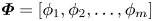 $\boldsymbol {\varPhi } = [\phi _1, \phi _2,\ldots ,\phi _m]$ and
  $\boldsymbol {\varSigma }$ takes singular values (
 $\sigma _1, \sigma _2,\ldots , \sigma _m$) along its diagonal. The singular value
  $\sigma _j^{2}$ indicates the energy level of mode
  $j$, and singular values are arranged from mode
  $1$ to mode
  $m$ in order of the amount of energy. The relative energy (energy fraction) captured by each mode can be computed as
 \begin{equation} \text{relative energy of mode }i= \frac{\sigma_i^{2}}{\sum_{j=1}^{m}\sigma_j^{2} } . \end{equation}
 According to the POD results, for each  $U^{*}$, the order of a modal shape corresponds to that of a harmonic mode with a clamped–clamped end condition (figure 8a–c). However, at each mode, the shape of the POD mode is displaced slightly in the streamwise direction from that of the harmonic mode due to fluid loading. While the first and second POD modes are dominant in terms of relative energy distribution, higher-order modes remain negligible in the entire
  $U^{*}$ range considered in this study (figure 8d). The relative energy level of the first mode at
  $U^{*} = 11.7$,
  $13.6$ and
  $16.6$ exceeds
  $0.4$, and that of the second mode is around
  $0.3$. The relative energy levels of higher-order modes are less than
  $0.1$. The dominance of the first and second modes in the snap-through oscillations seems to be different from the trend of a flapping flag with a fixed front end and a free rear end, which exhibits various vibrational modes depending on the dimensionless flow velocity and mass ratio (Tang & Païdoussis Reference Tang and Païdoussis2007; Eloy et al. Reference Eloy, Lagrange, Souilliez and Schouveiler2008; Michelin et al. Reference Michelin, Llewellyn Smith and Glover2008; Huang & Sung Reference Huang and Sung2010).

Figure 8. (a) First, (b) second and (c) third modal shapes at three flow velocities:  $U^{*} = 11.7$ (dotted line),
  $13.6$ (dashed line) and
  $16.6$ (dash-dotted line). In panels (a)–(c), the harmonic mode with a clamped–clamped end condition is shown by the solid line for comparison. (d) Relative energy of POD modes for
  $U^{*} = 11.7$ (blue),
  $13.6$ (red) and
  $16.6$ (green). Here
  $[L^{*}, H^{*}, m^{*}] = [0.75, 0.13, 0.95]$.
5.3. Bending energy
Because of its initial buckled configuration and quick snapping process, the sheet exhibits salient features regarding the elastic strain energy stored during the periodic oscillations. The elastic strain energy consists of bending energy and compressive force energy along the sheet. Because the sheet is assumed to be inextensible, the compression energy arises from the imposed end-shortening condition ( $L_0 < L$), and it is constant if
  $L^{*}$ is held fixed (Audoly & Pomeau Reference Audoly and Pomeau2010). Thus, only the bending energy of the sheet is considered in our examination of temporal variations in the strain energy. The bending energy per unit height is defined as
 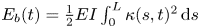 $E_b(t)=\tfrac {1}{2}EI\int _0^{L} \kappa (s,t)^{2}\, {\textrm {d}}s$, where
  $\kappa \ (=({\textrm {d}}^{2}y/{\textrm {d}x}^{2})/[1+({\textrm {d}y}/{\textrm {d}x})^{2}]^{{3}/{2}})$ is the curvature. The curvature was calculated with the dataset of positions acquired from the captured images. The sheet was discretized into
  $240$–
 $250$ segments along its length, and the central-difference scheme was used to obtain
  ${\textrm {d}y}/{\textrm {d}x}$ and
  $\textrm {d}^{2}y/{\textrm {d} x}^{2}$ for each segment; because the segments had the same length
  $\textrm {d}s$, different values of
  ${\textrm {d}x}$ were considered for the segments when
  ${\textrm {d}y}/{\textrm {d}x}$ and
  $\textrm {d}^{2}y/{\textrm {d}x}^{2}$ were discretized.
In figure 9(a), at the instant just before rapid snapping to the opposite side, the dimensionless bending energy  $E_b/E_{b,max}$ reaches its maximum value;
  $E_{b,max}$ is the maximum bending energy over 50 cycles in this study. Moreover, the phase just after the rapid snapping is complete corresponds to the minimum value of
  $E_b/E_{b,max}$. As shown by the light red and green regions, respectively, in figure 9(a), the time span required to release the bending energy generally becomes shorter than the time span required to store the bending energy, which results in a sawtooth waveform in the time history of the bending energy. The sharpness of the sawtooth waveform is found to be dependent on
  $L^{*}$. While the time history curve is sharp near the onset of snap-through for
  $L^{*} > 0.7$, the curve becomes blunt and exhibits plateaus for
  $L^{*} < 0.7$ (figure 11 in appendix B). Despite a change in the curve shape of the bending energy, rapid energy release during the snap-through process is consistently observed over a wide range of
  $L^{*}$.

Figure 9. (a) Dimensionless bending energy  $E_b/E_{b,max}$ stored in the sheet during snap-through oscillations;
  $E_{b,max}$ is the maximum bending energy over 50 cycles. The red dashed line denotes the level of
  $E_b/E_{b,max}$ at
  $U^{*} = 0$. A curve fitted from the experimental data (black circles) is denoted as the blue solid line. The insets describe the shape of the sheet at the phase of maximum bending energy (left) and minimum bending energy (right) for
  $U^{*} = 11.1$ as well as the initial shape for
  $U^{*} = 0$ (centre). Here
  $[L^{*}, H^{*}, m^{*}] = [0.75, 0.13, 0.95]$. (b) Ratio of bending energy at each free-stream velocity to bending energy at
  $U^{*} =0$:
  $E_b/E_{b,0}$. Circles denote the value of
  $E_b/E_{b,0}$ before
  $U^{*} = U^{*}_c$, and squares and triangles denote the maximum and minimum
  $E_b/E_{b,0}$ over successive cycles after
  $U^{*} = U^{*}_c$, respectively. Here
  $[L^{*}, H^{*}, m^{*}] = [0.60\text {--}0.86, 0.10\text {--}0.14, 0.76\text {--}1.08]$.
As  $U^{*}/U^{*}_c$ increases from zero up to unity in the equilibrium state (
 $U^{*}/U^{*}_c < 1$), the ratio of the bending energy at a given flow velocity to the bending energy at
  $U^{*} = 0$,
  $E_b/E_{b,0}$, gradually grows from
  $1.0$ to
  $1.6$ owing to enhanced deflection of the sheet along the flow direction. Regardless of the variations in
  $L^{*}$, the
  $E_b/E_{b,0}$ values are distributed narrowly at a given
  $U^{*}/U^{*}_c$ (figure 9b). In the post-equilibrium state (
 $U^{*}/U^{*}_c \geq 1$), the maximum and minimum values of
  $E_b/E_{b,0}$ over successive cycles form separate groups around
  $2.5$ and
  $1.0$, respectively. For a given
  $U^{*}/U^{*}_c$, the difference in the bending energy between the two extreme phases,
  ${\rm \Delta} E_b/E_{b,0}\ (=[E_{b,max} - E_{b,min}]/E_{b,0})$, increases slightly as
  $L^{*}$ increases, which implies that the energy release by the snapping is more effective as
  $L^{*}$ is closer to unity.
During the periodic oscillations, the instantaneous configurations of the sheet at the upper and lower energy limits remain similar to the second and first modal shapes, respectively (figure 9b), and this trend is universal for all  $U^{*}$ values considered in this study; for example, see the insets of figure 9(a) and figure 11 in appendix B. The higher-order modes are not dominant at any phase of the oscillations. If the higher-order modal shape was dominant, the curvature of the sheet constrained by the clamped ends would be much greater than that of the second modal shape, resulting in a dramatic growth in the bending energy. Accordingly, although both maximum and minimum values of the bending energy tend to increase slightly with
  $U^{*}$ in limit-cycle oscillation, each of them is confined within a narrow range without a notable jump in energy level: the maximum
  $E_b/E_{b,0}$ ranges from
  $2.3$ to
  $3.0$ and the minimum
  $E_b/E_{b,0}$ ranges from
  $0.8$ to
  $1.2$.
The aforementioned characteristics of the bending energy are in stark contrast to those of the flag models, which experience smooth temporal variations in bending energy during periodic oscillations. Owing to the buckled configuration, the ratio of minimum bending energy to maximum bending energy remains at least  $40\,\%$ in the snap-through model (figure 9a). Meanwhile, it is almost zero in the flag model (Gurugubelli & Jaiman Reference Gurugubelli and Jaiman2015) because the flapping flag becomes almost straight at some point. Furthermore, unlike the flag model, which exhibits similar time spans for energy storage and release, the snap-through model displays a shorter time span for energy release than for energy storage.
6. Concluding remarks
We have reported the novel behaviour of the flow-induced snap-through of a buckled sheet and several notable differences from the well-known responses of flapping flags. Experimental measurements in wind and water tunnels and low-order numerical simulations using the nonlinear beam equation and quasi-steady fluid dynamics have clarified the effects of the length ratio and mass ratio on the onset condition of instability and revealed that the transition to the limit-cycle oscillation is due to the divergence instability mechanism. Because the sheet is clamped at both ends, only the first and second modes are dominant as the flow velocity changes. Over an oscillation cycle, the bending energy stored in the sheet attains a maximum immediately before snapping to the opposite side, and decreases suddenly and reaches a minimum just after the snapping process is complete.
In this study, periodic snap-through dynamics with a large amplitude were investigated for high-Reynolds-number flows with fluid kinetic energy harvesting applications in mind. The quick snapping process, robust oscillations over a broad range of flow velocities and negligible density effects of the surrounding fluid on bifurcation offer insights into the potential application of flow-induced snap-through to small-scale energy harvesters. In future, we plan to explore the optimal operational and design conditions of a snap-through-based energy harvesting system from the perspective of the fluid–structure interactions.
Supplementary movie
A supplementary movie is available at https://doi.org/10.1017/jfm.2021.57.
Funding
This research was supported by the Basic Science Research Program through the National Research Foundation of Korea (NRF) funded by the Ministry of Science and ICT (NRF-2017R1E1A1A01074704, NRF-2020R1A2C2102232).
Declaration of interest
The authors report no conflict of interest.
Appendix A. Comparison between nonlinear and linear equations
The steady and linearized Euler–Bernoulli beam equation per unit height in the absence of external loading is
 \begin{equation} B\frac{{\textrm{d}}^{4}y}{{\textrm{d} x}^{4}}+P_{0}\frac{{\textrm{d}}^{2}y}{{\textrm{d} x}^{2}}=0, \end{equation}
which is valid for small deflections. Here  $B$ is the bending rigidity of the sheet per unit height,
  $P_{0}$ is the compressive force per unit height with no external force and
  $y$ is the transverse displacement of the sheet. With four boundary conditions at both edges (
 $y|_{x = 0,L_0} = 0$,
 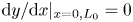 ${\textrm {d} y}/{\textrm {d} x}|_{x = 0, L_0} = 0$), the solution of (A1) provides a buckled shape:
 \begin{equation} y(x) = C\left(1-\cos\frac{2{\rm \pi}}{L_0}x\right),\end{equation}
where the constant  $C$ is
  $w_0/2$ from the relation
  $y(L_0/2) = w_0$. The
  $w_0$ value for given
  $L$ and
  $L_0$ (and thus
  $L^{*}$) is then numerically determined by the constraint on the length of the buckled sheet (A3):
 \begin{equation} \int_{0}^{L_0}\left[1+\left(\frac{\textrm{d} y}{\textrm{d} x}\right)^{2}\right]^{{1}/{2}}{\textrm{d} x} = L. \end{equation}
When  $L^{*} = 0.85$, (A2) predicts a quite accurate buckled shape in the absence of flow, compared with the actual shape observed in the experiment (figure 10a). However, the accuracy decreases as
  $L^{*}$ decreases, and the shape obtained by (A1) deviates significantly from the actual shape for a small
  $L^{*}$; the maximum transverse displacement
  $w_0$ also deviates, as shown in figure 10(b). In contrast, the solution of the nonlinear elastica theory expressed in (3.1) is in excellent agreement with the real shape, regardless of the
  $L^{*}$ value (figure 10a,b).

Figure 10. (a) Initial shapes of the buckled sheet with no fluid flow for several length ratios  $L^{*}$. Theoretical solutions obtained by the linear Euler–Bernoulli beam equation ((A1), red) and the nonlinear elastica theory ((3.1), blue) are compared with images captured from experiments (black). (b) Comparison of maximum transverse displacement
  $w_0$ obtained from the linear Euler–Bernoulli equation (red), elastica theory (blue) and experimental measurements (black circles). (c) Compressive force
  $P_0/P_{cr}$ applied on the buckled sheet with no fluid flow, acquired by solving equation (3.1).
For small deflection ( $|{\textrm {d} y}/{\textrm {d} x}|\ll 1$), the constant
  $C$ in (A2) can be determined analytically by approximating (A3) as
 \begin{equation} \int_{0}^{L_0}\left[1+\frac{1}{2}\left(\frac{\textrm{d} y}{\textrm{d} x}\right)^{2}\right]{\textrm{d} x} \approx L. \end{equation}
From (A2) and (A4),  $C$ is
  $[L_0(L-L_0)]^{{1}/{2}}/{\rm \pi}$, and
  $w_0/L$ can be expressed as
 \begin{equation} \frac{w_0}{L} = \frac{2}{\rm \pi}[L^{*}(1-L^{*})]^{{1}/{2}}.\end{equation}
On the other hand,  $P_0$ can be obtained from the numerical solution of (3.1) as a function of
  $L^{*}$ (figure 10c). When
  $L^{*}$ approaches unity,
  $P_0$ converges to the critical buckling load
  $P_{cr}\ (=4{\rm \pi} ^{2} B/L^{2})$. As
  $L^{*}$ decreases,
  $P_0$ increases, indicating that a larger compressive force is required to make a more buckled sheet.
Appendix B. Time history of bending energy
Figure 11 shows that the sharpness of the time history curve of the bending energy varies with  $L^{*}$ as explained in § 5.3. For
  $L^{*} > 0.7$, which exhibits a sharp decrease in
  $E_b/E_{b,max}$ during snapping (figure 11a,b), the sheet begins to snap at a maximum bending energy level. In contrast, the bending energy curve for the sheet with
  $L^{*} = 0.6$ (figure 11d) has a plateau instead of a sharp peak. The sheet does not snap at the moment when the sheet attains the maximum bending energy, but some time is taken before the snapping is initiated.

Figure 11. Time history of dimensionless bending energy  $E_b/E_{b,max}$ for: (a)
  $L^{*} = 0.86\ (H^{*} = 0.14,\ $
  $m^{*} = 1.08)$; (b)
  $L^{*} = 0.75\ (H^{*} = 0.13,\ m^{*} = 0.95)$; (c)
  $L^{*} = 0.67\ (H^{*} = 0.11,\ m^{*} = 0.84)$; and (d)
  $L^{*} = 0.60\ (H^{*} = 0.10,\ m^{*} = 0.76)$. The red dashed line is
  $E_b/E_{b,max}$ of an initial buckled sheet with no flow. A curve fitted to the experimental data (black circles) is denoted as the blue solid line. The two insets below each panel are the sheet shapes with minimum (left) and maximum (right) bending energy, respectively. For each
  $L^{*}$, the data were obtained near the critical velocity: (a)
  $U^{*} = 9.8$; (b)
  $U^{*} = 11.1$; (c)
  $U^{*} = 12.6$; and (d)
  $U^{*} = 13.4$.


