


1. Introduction
Turbulence under system rotation often occurs in many geophysical, astrophysical and engineering problems. In a rotating frame fixed with solid walls, such as a turbomachine rotor, turbulence will be strongly influenced by the Coriolis force and exhibit complex behaviours. Owing to the simple geometry and high similarity with various turbomachinery flows, spanwise rotating plane Poiseuille flow (RPPF) has been regarded as one of the most important canonical models of rotating wall-bounded shear flows (Johnston Reference Johnston1998; Jakirlic, Hanjalic & Tropea Reference Jakirlic, Hanjalic and Tropea2002) and has been intensively investigated.
Johnston, Halleent & Lezius (Reference Johnston, Halleent and Lezius1972) first investigated the turbulent RPPF by experiments and found that turbulence is enhanced near the pressure side, while suppressed near the suction side. Here the definitions of the pressure and the suction side originated from the difference of mean pressure between two walls caused by the Coriolis force corresponding to the mean velocity (Johnston Reference Johnston1998). Following the thermal analogy introduced by Bradshaw (Reference Bradshaw1969), the region corresponding to unstable/stable stratification is adjacent to the pressure/suction side and, straightforwardly, the pressure/suction side is also called the unstable/stable side. In addition, a local linear mean streamwise velocity profile with a slope of approximately twice that of the spanwise angular velocity  $\varOmega _z^*$ as well as large-scale streamwise Taylor–Görtler vortices (roll cells) were observed near the unstable side by Johnston et al. (Reference Johnston, Halleent and Lezius1972). Matsubara & Alfredsson (Reference Matsubara and Alfredsson1996) measured the heat and momentum transfer in RPPF, and found that the rotation could strongly increase the heat transfer by almost
  $100\,\%$, while the classic Reynolds analogy between momentum and heat transfer is no longer valid in RPPF. Nakabayashi & Kitoh (Reference Nakabayashi and Kitoh1996, Reference Nakabayashi and Kitoh2005) also investigated RPPF at relatively lower Reynolds number (
 $Re=U_b^*h^*/\nu ^*$) and rotation number (
 $Ro=2\varOmega _z^*h^*/U_b^*$) experimentally, and the measured turbulence statistics were discussed with reference to the dimensional analysis. Here,
  $U_b^*$ is the bulk mean velocity,
  $\nu ^*$ is the kinematic viscosity and
  $h^*$ is the half-width of the channel. Other experimental studies include, but are not limited to, Maciel et al. (Reference Maciel, Picard, Yan, Gleyzes and Dumas2003) and Visscher et al. (Reference Visscher, Andersson, Barri, Didelle, Viboud, Sous and Sommeria2011).
Owing to the difficulty of globally accurate experimental measurement of fully developed turbulent RPPF, and the fast development of computer hardware and software, direct numerical simulations (DNSs) are becoming prevalent tools for the investigation of turbulent RPPF at low and medium Reynolds numbers. Kristoffersen & Andersson (Reference Kristoffersen and Andersson1993) first performed DNS to study the turbulent RPPF with weak to medium rotations, and observed large-scale roll cells and the local  $2\varOmega _z^*$-slope linear mean velocity profile, which were consistent with former experimental results. Since then, many DNS studies have been carried out by the community to investigate the turbulent statistics and flow physics in RPPF. Nagano & Hattori (Reference Nagano and Hattori2003) studied the heat transport in RPPF through DNS and used the results to assess turbulence models. Grundestam, Wallin & Johansson (Reference Grundestam, Wallin and Johansson2008) focused on DNSs with medium to high
  $Ro$ at a fixed global friction Reynolds number
  $Re_\tau =u_\tau ^*h^*/\nu ^*=180$ (
 $u_\tau ^*$ is the global friction velocity), and found that the bulk flow was monotonically increasing with
  $Ro$ in the
  $Ro$ range investigated and that the flow will be fully relaminarized at the laminar limit
  $Ro=3.0$. Brethouwer et al. (Reference Brethouwer, Schlatter, Duguet, Henningson and Johansson2014) conducted DNSs with a wide range of
  $Ro$ and
  $Re=20\,000$, and observed cyclic instabilities at large
  $Ro$ caused by the growth and breakdown of Tollmien–Schlichting (TS) waves. Xia, Shi & Chen (Reference Xia, Shi and Chen2016) also performed DNSs with a wide range of
  $Ro_\tau =2\varOmega _z^*h^*/u_\tau ^*$ at
  $Re_\tau =180$, and observed linear profiles for the Reynolds shear stress
  $\langle u'v'\rangle$ and the production term of
  $\langle u'u'\rangle$, where the former has a unit slope and the latter has a
  $-2Ro_\tau$ slope. Hsieh & Biringen (Reference Hsieh and Biringen2016) investigated the influence of small computational domains on turbulence statistics and flow structures, and found that a small spanwise size of computational domain will change the shape of roll cells, which will make the turbulence statistics deviate from those computed using large computational domains. Other DNS studies include, but are not limited to, Liu & Lu (Reference Liu and Lu2007), Yang & Wu (Reference Yang and Wu2012), Wallin, Grundestam & Johansson (Reference Wallin, Grundestam and Johansson2013), Dai, Huang & Xu (Reference Dai, Huang and Xu2016), Brethouwer (Reference Brethouwer2016, Reference Brethouwer2017, Reference Brethouwer2018, Reference Brethouwer2019) and Xia, Brethouwer & Chen (Reference Xia, Brethouwer and Chen2018a).
Although RPPF is studied intensively, not all important flow structures in RPPF are well identified and analysed. Despite the vortices, the streak structures and the Taylor–Görtler vortices (roll cells) can generally be observed on the unstable side in many experimental and numerical studies of RPPF (Grundestam et al. Reference Grundestam, Wallin and Johansson2008; Brethouwer Reference Brethouwer2017). Strong evidence has shown that roll cells exist in RPPF at low  $Re$ when
  $Ro\lesssim 0.6$, and they are less certain and much harder to detect owing to them being non-stationary in space and smaller size at higher
  $Ro$ (Brethouwer Reference Brethouwer2017). At higher
  $Re$ and
  $Ro$, the roll cells are hardly discernable, and oblique turbulent–laminar bands and cyclic turbulent bursts have been reported recently (Brethouwer et al. Reference Brethouwer, Schlatter, Duguet, Henningson and Johansson2014; Brethouwer Reference Brethouwer2016, Reference Brethouwer2017). These flow structures were previously used to explain the observed flow phenomenon and statistics. For examples, Brethouwer (Reference Brethouwer2017) proposed that the roll cells can modulate the near-wall dynamics on the unstable side according to the clustering of intense vortices in streamwise near-wall streaks shown by the flow visualization, while Brethouwer (Reference Brethouwer2016) attributed the strong temporal fluctuations of the mean wall shear stress and volume-averaged turbulent kinetic energy at high
  $Re$ and
  $Ro$ to the cyclic turbulent bursts. However, not all flow phenomenon and statistics in RPPF can be explained by using the above-discussed flow structures. It is well accepted that the turbulence would become progressively weaker on the stable side with increasing rotation speed (Brethouwer Reference Brethouwer2017). Nevertheless, the root-mean-square (r.m.s.) values of the streamwise velocity fluctuations near the stable side at higher rotation speed do not disappear but have values which are very close to those near the unstable side, as shown by figure 11(a) in Grundestam et al. (Reference Grundestam, Wallin and Johansson2008), figure 3 in Xia et al. (Reference Xia, Shi and Chen2016), figure 6 in Brethouwer (Reference Brethouwer2017) and figure 8(a) in the present paper. These results imply that some flow structures should exist near the stable side and they have not been identified before.
In our previous work, Zhang et al. (Reference Zhang, Xia, Shi and Chen2019) introduced a two-dimensional three-component (2D3C) model to simplify the three-dimensional (3-D) RPPF by assuming that the velocity is invariant in the streamwise direction. The 2D3C model is equivalent to a two-dimensional (2-D) penetrative convection mathematically based on the thermal analogy. Hereafter, the RPPF with the 2D3C model will be called ‘2-D RPPF’ for simplicity. In the results, Zhang et al. (Reference Zhang, Xia, Shi and Chen2019) observed a local  $Ro_\tau$-slope of the mean streamwise velocity profile and a local unit slope of the Reynolds shear stress in 2-D RPPF, which are the same as those observed in the fully 3-D RPPF, which indicates that some important features in the fully 3-D RPPF could be dominated by 2-D mechanisms in the 2-D RPPF. In 2-D penetrative convection problems, Wang et al. (Reference Wang, Zhou, Wan and Sun2019a) observed plumes in the flow field, while Lecoanet et al. (Reference Lecoanet, Le Bars, Burns, Vasil, Brown, Quataert and Oishi2015) and Toppaladoddi & Wettlaufer (Reference Toppaladoddi and Wettlaufer2018) showed that internal gravity waves exist in the stably stratified region. Therefore, the local existence of plumes and waves in 2-D RPPF could be expected. Considering the similarity between a 2-D RPPF and a fully 3-D RPPF, it is also intuitive to examine the existence of plume and wave structures in fully 3-D RPPF. If plume structures exist in RPPF, detailed investigation on such structures may inspire possible control strategies in RPPF because the control of plumes is an effective strategy in thermal convection (Zhang et al. Reference Zhang, Sun, Bao and Zhou2018; Zhu et al. Reference Zhu, Stevens, Shishkina, Verzicco and Lohse2019; Zhang et al. Reference Zhang, Chen, Xia, Xi, Zhou and Chen2021). Meanwhile, the existence of waves may help clarify the mechanisms behind flow visualizations and statistics mentioned above. It should be noted that near-wall plumes were once identified by Ostilla-Mónico et al. (Reference Ostilla-Mónico, Van Der Poel, Verzicco, Grossmann and Lohse2014), van der Veen et al. (Reference van der Veen, Huisman, Merbold, Harlander, Egbers, Lohse and Sun2016) and Sacco, Verzicco & Ostilla-Mónico (Reference Sacco, Verzicco and Ostilla-Mónico2019) in turbulent Taylor–Couette flow (TCF) based on the analogy between rotating shear flows and thermal convection.
In this paper, we will explore the flow structures on both stable and unstable sides in RPPF with inspiration from the typical structures that exist in penetrative convection. The remainder of the paper is organized as follows. The governing equations, thermal analogy and numerical set-up of RPPF will be introduced in § 2. Based on theoretical analysis and DNS results, discussions on important flow structures in RPPF will be presented in § 3. Finally, the present work will be summarized in § 4.
2. Governing equations and numerical description
2.1. Three-dimensional equations
As sketched in figure 1, the incompressible fluid is bounded by two parallel and infinite plates located at  $y^*=\pm h^*$. The flow is driven by a constant mean pressure gradient
  $\textrm {d} P^*/{\textrm {d}\kern0.06em x}^*$ along the
  $x$ direction (streamwise direction). The whole system rotates with a constant angular velocity
  $\varOmega _z^*$ along the
  $z$ direction (spanwise direction). In this paper,
  $\varOmega _z^*$ is assumed to be positive and the lower/upper wall is the pressure (unstable)/suction (stable) side. A passive scalar
  $\phi ^*$ is defined in the fluid region, and has constant values
  $\phi _u^*$ and
  $\phi _l^*$ at the upper and lower walls, respectively. The constant reference density is
  $\rho ^*$; the kinematic viscosity is
  $\nu ^*$; the scalar diffusivity is
  $\kappa ^*$; the reference length scale is the channel half-width
  $h^*$; the reference scale of
  $\phi ^*$ is
  $\varDelta \phi ^*=\phi _l^*-\phi _u^*$; the reference velocity scale is the global friction velocity
  $u_\tau ^*$ in a statistically steady state, which is equal to
  $\sqrt {-\textrm {d} P^*/{\textrm {d}\kern0.06em x}^*(h^*/\rho ^*)}$. Using these reference quantities, the non-dimensionalized governing equations and boundary conditions can be written as follows:
 \begin{equation} \left.\begin{gathered} \boldsymbol{\nabla}\boldsymbol{\cdot}\boldsymbol{u}=0,\\ \frac{\partial\boldsymbol{u}}{\partial t}+\boldsymbol{u}\boldsymbol{\cdot}\boldsymbol{\nabla}\boldsymbol{u}={-}\boldsymbol{\nabla} p+Re_\tau^{{-}1}\nabla^2\boldsymbol{u}-Ro_\tau\boldsymbol{e}_z\times\boldsymbol{u},\\ \frac{\partial\phi}{\partial t}+\boldsymbol{u}\boldsymbol{\cdot}\boldsymbol{\nabla}\phi=Pr^{{-}1}Re_\tau^{{-}1}\nabla^2\phi,\\ y={-}1:\ \boldsymbol{u}=0,\quad \phi=1,\\ y={+}1:\ \boldsymbol{u}=0,\quad \phi=0. \end{gathered}\right\}\end{equation}
Here,  $Re_\tau =u_\tau ^*h^*/\nu ^*$ is the global friction Reynolds number;
  $Ro_\tau =2\varOmega _z^*h^*/u_\tau ^*$ is the global friction rotation number and
  $Pr=\nu ^*/\kappa ^*$ is the Prandtl number.

Figure 1. Sketch of the three-dimensional spanwise rotating plane Poiseuille flow.
2.2. Two-dimensional equations and thermal analogy
Following Zhang et al. (Reference Zhang, Xia, Shi and Chen2019), the 2-D equations (2D3C model) are defined as the governing equations with extra constraints  $\partial \boldsymbol {u}/\partial x=0$ and
  $\partial \phi /\partial x=0$:
 \begin{equation} \left.\begin{gathered} \frac{\partial v}{\partial y}+\frac{\partial w}{\partial z}=0,\\ \frac{\partial u}{\partial t}+v\frac{\partial u}{\partial y}+w\frac{\partial u}{\partial z} ={-}\frac{\textrm{d} P}{\textrm{d}x}+Re_\tau^{{-}1}\left(\frac{\partial^2 u}{\partial y^2}+ \frac{\partial^2 u}{\partial z^2}\right)+Ro_\tau v,\\ \frac{\partial v}{\partial t}+v\frac{\partial v}{\partial y}+w\frac{\partial v}{\partial z} ={-}\frac{\partial p}{\partial y}+Re_\tau^{{-}1}\left(\frac{\partial^2 v}{\partial y^2}+ \frac{\partial^2 v}{\partial z^2}\right)-Ro_\tau u,\\ \frac{\partial w}{\partial t}+v\frac{\partial w}{\partial y}+w\frac{\partial w}{\partial z} ={-}\frac{\partial p}{\partial z}+Re_\tau^{{-}1}\left(\frac{\partial^2 w}{\partial y^2}+ \frac{\partial^2 w}{\partial z^2}\right),\\ \frac{\partial\phi}{\partial t}+v\frac{\partial \phi}{\partial y}+w\frac{\partial \phi}{\partial z} =Pr^{{-}1}Re_\tau^{{-}1}\left(\frac{\partial^2\phi}{\partial y^2}+\frac{\partial^2\phi}{\partial z^2}\right), \end{gathered}\right\}\end{equation}
with the same boundary conditions as (2.1).
Following Tanaka et al. (Reference Tanaka, Kida, Yanase and Kawahara2000) and Zhang et al. (Reference Zhang, Xia, Shi and Chen2019), by defining a new variable  $\theta =-u+Ro_\tau y$ and letting
  $\hat {p}=p+Ro_\tau ^2y^2/2$, (2.2) can be written as the following equivalent governing equations of a 2-D penetrative convection with an internal heat sink. For simplicity, in the following, the new variable
  $\theta$ will be called ‘temperature’.
 \begin{equation} \left.\begin{gathered} \frac{\partial v}{\partial y}+\frac{\partial w}{\partial z}=0,\\ \frac{\partial v}{\partial t}+v\frac{\partial v}{\partial y}+w\frac{\partial v}{\partial z} ={-}\frac{\partial\hat{p}}{\partial y}+Re_\tau^{{-}1}\left(\frac{\partial^2 v}{\partial y^2}+ \frac{\partial^2 v}{\partial z^2}\right)+Ro_\tau\theta,\\ \frac{\partial w}{\partial t}+v\frac{\partial w}{\partial y}+w\frac{\partial w}{\partial z} ={-}\frac{\partial\hat{p}}{\partial z}+Re_\tau^{{-}1}\left(\frac{\partial^2 w}{\partial y^2}+ \frac{\partial^2 w}{\partial z^2}\right),\\ \frac{\partial\theta}{\partial t}+v\frac{\partial\theta}{\partial y}+w\frac{\partial\theta}{\partial z} =\frac{\textrm{d} P}{\textrm{d}x}+Re_\tau^{{-}1}\left(\frac{\partial^2\theta}{\partial y^2}+ \frac{\partial^2\theta}{\partial z^2}\right),\\ \frac{\partial\phi}{\partial t}+v\frac{\partial \phi}{\partial y}+w\frac{\partial \phi}{\partial z} =Pr^{{-}1}Re_\tau^{{-}1}\left(\frac{\partial^2\phi}{\partial y^2}+\frac{\partial^2\phi}{\partial z^2}\right),\\ y={-}1:\ v=w=0,\quad \theta={-}Ro_\tau,\quad \phi=1,\\ y={+}1:\ v=w=0,\quad \theta={+}Ro_\tau,\quad \phi=0. \end{gathered}\right\}\end{equation}
Apparently, the equivalent penetrative convection system has viscosity  $\hat {\nu }=Re^{-1}_\tau$, thermal diffusivity
  $\hat {\alpha }=Re^{-1}_\tau$, uniform heat sink
  $\hat {q}=-\textrm {d} P/{\textrm {d}\kern0.06em x}=1$, and the product of gravitational acceleration and thermal expansion coefficient
  $\hat {g}\hat {\beta }=Ro_\tau$. Behind the buoyancy term
  $\hat {g}\hat {\beta }\theta \boldsymbol {e}_y$, the equation of state is
  $(\hat {\rho }-\hat {\rho }_0)/\hat {\rho }_0=-\hat {\beta }\theta$, and hence the mean ‘density’ profile is
  $\langle \hat {\rho }\rangle =(1-\hat {\beta }\theta )\hat {\rho }_0$.
2.3. Numerical set-up
Both the 3-D and 2-D equations are solved using a second-order central-difference code AFiD (Van Der Poel et al. Reference Van Der Poel, Ostilla-Mónico, Donners and Verzicco2015) with some modifications. Flow variables are defined on a staggered grid. The Poisson equation of the pressure is decoupled using the discrete Fourier transform in the  $x$ and
  $z$ direction, and solved using a tridiagonal solver. The time marching is realized with the explicit second-order Adams–Bashforth scheme. Because AFiD is designed for simulating Rayleigh–Bénard convection, the
  $\phi$ equation could be solved well. A 3-D simulation at
  $Re_\tau =180$ and
  $Ro_\tau =10$ is performed to verify the present modified code for RPPF simulation. Figure 2(a) shows that the viscous and Reynolds shear stresses computed using the present code match very well with the results in Zhang et al. (Reference Zhang, Xia, Shi and Chen2019), which were obtained with a highly accurate Fourier–Chebyshev pesudo-spectral method. In addition, two 3-D simulations are performed at the same
  $Re_\tau =180$ and
  $Ro_\tau =120$ but with different grid resolutions. The one, which is considered as the basic grid resolution, has grid size
  $N_x\times N_y\times N_z=256\times 192\times 256$, and the other is refined to
  $N_x\times N_y\times N_z=384\times 256\times 384$. Figure 2(b) shows the probability density functions (p.d.f.s) of the normalized streamwise velocity fluctuation at three different
  $y$ from the two cases, and it is seen that the p.d.f.s with different resolutions match with each other very well at all three locations, which suggests that the basic resolution is fine enough for high
  $Ro_\tau$ simulations at
  $Re_\tau =180$. The basic parameters of all 3-D and 2-D simulations are listed in table 1, which shows that the present grid resolution is much finer than that used by Kristoffersen & Andersson (Reference Kristoffersen and Andersson1993) in wall units.

Figure 2. (a) Comparison of shear stresses in the 3-D and  $Ro_\tau =10$ case with those in Zhang et al. (Reference Zhang, Xia, Shi and Chen2019); (b) comparison of the p.d.f.s of normalized streamwise velocity fluctuation at different
  $y$ in the 3-D
  $Ro_\tau =120$ case with the basic resolution (symbols) and the refined resolution (lines). Each pair of line and symbols in panel (b) is shifted upwards from its lower neighbour by a factor of 10.
Table 1. Basic physical and computational parameters of 3-D and 2-D simulation cases. The wall units are defined using  $u_\tau ^*$.

3. Results
3.1. Plumes
In penetrative convection, plumes are one kind of the typical structures (Lecoanet et al. Reference Lecoanet, Le Bars, Burns, Vasil, Brown, Quataert and Oishi2015; Toppaladoddi & Wettlaufer Reference Toppaladoddi and Wettlaufer2018; Wang et al. Reference Wang, Zhou, Wan and Sun2019a). As shown in § 2.2, where 2-D RPPF is mathematically equivalent to a penetrative convection with internal heat sink, plumes should exist in 2-D RPPF. Such existence can be examined with flow visualizations and statistical analysis.
Figure 3 shows the contours of  $u'$ in the
  $y$–
$y$– $z$ plane from the 2-D RPPF simulations at different
  $Ro_\tau$ (see also the supplementary movie 1 and movie 2 available at https://doi.org/10.1017/jfm.2021.1073 for
  $Ro_\tau =5$ and 40, respectively). Here,
  $a'=a-\langle a\rangle$ denotes the fluctuation of any field
  $a$ with
  $\langle a\rangle$ denoting the average of
  $a$ in homogeneous directions and
  $t$. To view the structures more clearly, the dashed and dash–dotted lines are shown to denote the horizontal locations
  $y_1$ and
  $y_2$ with
  $N_b(y_1)=0.1N_b(-1)$ and
  $N_b(y_2)=0.1N_b(1)$, respectively. Here,
  $N_b(y)=[-Ro_\tau (\textrm {d}\langle u\rangle /{\textrm {d}y}-Ro_\tau )]^{1/2}$, with its imaginary part
  $\text {Im}[N_b]\leq 0$ chosen, is the complex characteristic frequency of the simplified system (see § 3.2 for more information). Using
  $y_1$ and
  $y_2$ to divide the fluid domain has strong physical significance. First, the flow below the plane
  $y=y_1$ can be strongly destabilized because a characteristic growth rate
  $|\text {Im}[N_b]|$ there is above
  $10\,\%$ of its maximum value
  $|\text {Im}[N_b(-1)]|$ over the channel. Second, the flow above the plane
  $y=y_2$ may be rapidly oscillating because a characteristic oscillation frequency
  $\text {Re}[N_b]$ there is above
  $10\,\%$ of its maximum value
  $\text {Re}[N_b(1)]$ over the channel (
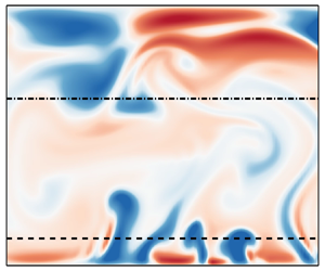
 $\text {Re}[\cdot ]$ denotes taking the real part). From figure 3 it is evident that there are plume-like structures generated from the unstable side below the dashed lines in 2-D RPPF, which carry negative
  $u'$ (positive
  $\theta '$).

Figure 3. Contours of  $u'$ in
  $y$–
$y$– $z$ planes of instantaneous fields from 2-D simulations: (a)
  $Ro_\tau =1$; (b)
  $Ro_\tau =5$; (c)
  $Ro_\tau =40$; (d)
  $Ro_\tau =120$. The dashed and dash–dotted lines denote the horizontal locations at
  $y=y_1$ and
  $y=y_2$ with
  $N_b(y_1)=0.1N_b(-1)$ and
  $N_b(y_2)=0.1N_b(1)$, respectively.
To study the statistical characteristics of flow structures in RPPF near the unstable side, the p.d.f. of turbulence fluctuations should be analysed. Figure 4(a–c) shows the p.d.f.s of normalized  $\theta '=-u'$ at different heights in 2-D RPPF. It can be seen that all p.d.f.s obtained below the plane
  $y=y_2$ significantly deviate from the symmetric Gaussian distribution and may show locally exponential behaviours (linear in logarithmic vertical coordinate). Inspired by the statistical theory of Rayleigh–Bénard convection introduced by Wang, He & Tong (Reference Wang, He and Tong2019b), where turbulent fluctuations in Rayleigh–Bénard convection can be decomposed into the contribution from a homogeneous background turbulence and the contribution from the thermal plumes, the p.d.f.s of normalized
  $\theta '=-u'$ near the unstable region (below the plane
  $y=y_2$) can be modelled.

Figure 4. The p.d.f.s of normalized  $-u'$ and
  $v'$ at different heights in 2-D cases: (a–c)
  $-u'/u'_{\textit{rms}}$; (d–f)
  $v'/v'_{\textit{rms}}$. The sampling planes are chosen with
  $N_b(y)$ equal to (a,d)
  $0.3N_b(-1)$; (b,e)
  $0$; (c,f)
  $0.3N_b(1)$. Symbols represent simulation data; lines in (a,b,d,e) represent the fitting curves using the theoretical model (3.5); lines in (c,f) represent the normalized Gaussian distribution. For clarity, each dataset has been shifted upwards from its lower neighbour by a factor of 10.
For a specific scalar fluctuation  $\xi$ with
  $\langle \xi \rangle =0$, the background turbulence could be quantified by a Gaussian distribution:
 \begin{equation} P_b(\xi)=\left(2{\rm \pi}\sigma^2\right)^{{-}1/2}\exp\left({-\frac{\xi^2}{2\sigma^2}}\right), \end{equation}
with  $\sigma$ being the standard deviation of the Gaussian distribution. The contribution of plumes could be quantified by an exponential distribution with some modifications:
 \begin{equation} \tilde{P}_p(\xi)=(1-\alpha)\delta(\xi)+\frac{\alpha\beta }{1-\textrm{e}^{-\beta M}}\,\textrm{e}^{-\beta\xi} \left[H(\xi)-H(\xi-M)\right]. \end{equation}
Here,  $\delta$ is the Dirac delta function;
  $H$ is the Heaviside function;
  $\beta$ is the coefficient controlling the exponential decay;
  $0\leq \alpha \leq 1$ quantifies the intermittency of plumes; and
  $M$ is the maximum amplitude possible for
  $\xi$ with respect to the plumes, which is introduced based on the physical consideration that the plumes cannot induce an infinite amplitude of
  $\xi$. There are two modifications in (3.2) based on the classical exponential distribution
  $\beta \,\textrm {e}^{-\beta \xi }H(\xi )$. The first one is adding the term
  $(1-\alpha )\delta (\xi )$ (Wang et al. Reference Wang, He and Tong2019b), which means that during some time and in some places, plumes are absent and the instantaneous plume strength should be zero. The second modification is substituting
  $H(\xi )$ with
  $H(\xi )-H(\xi -M)$ (newly introduced in the present work), which means that in addition to being non-negative,
  $\xi$ should also be less than
  $M$. Because the distribution (3.2) has a non-zero expectation,
 \begin{equation} \mu=\frac{\alpha\left[1-\textrm{e}^{-\beta M}(\beta M+1)\right]}{\beta\left(1-\textrm{e}^{-\beta M}\right)}, \end{equation}
the exponential distribution with zero expectation should be
 \begin{align} P_p(\xi)&=\tilde{P}_p(\xi+\mu) \nonumber\\ &=(1-\alpha)\delta(\xi+\mu)+\frac{\alpha\beta \,\textrm{e}^{-\beta\mu}}{1-\textrm{e}^{-\beta M}} \textrm{e}^{-\beta\xi}\left[H(\xi+\mu)-H(\xi+\mu-M)\right]. \end{align}
Therefore, the total distribution of  $\xi$ should be the convolution of
  $P_b$ and
  $P_p$ (Wang et al. Reference Wang, He and Tong2019b):
 \begin{align} P(\xi)&=P_b*P_p \nonumber\\ &=\int_{-\infty}^\infty{P_b(s)P_p(\xi-s)\,\textrm{d} s} \nonumber\\ &=\frac{1-\alpha}{\sqrt{2{\rm \pi}}\sigma}\exp\left({-\frac{(\xi+\mu)^2}{2\sigma^2}}\right) \nonumber\\ &\quad +\frac{1}{2}\frac{\alpha\beta \exp\left({\dfrac{\sigma^2\beta^2}{2}-\beta\mu}\right)}{1-\textrm{e}^{-\beta M}} \textrm{e}^{-\beta\xi}\left[\text{erf}\left(\frac{\xi+\mu-\sigma^2\beta}{\sqrt{2}\sigma}\right) \right.\nonumber\\ &\quad \left.-\text{erf}\left(\frac{\xi+\mu-\sigma^2\beta-M}{\sqrt{2}\sigma}\right)\right]. \end{align}
 We fit the p.d.f.s of  $\theta '=-u'$ from different
  $Ro_\tau$ at different locations with
  $y< y_2$ using the above theoretical distribution (3.5) (the detailed parameters are listed in Appendix A) and the fitted curves are shown in figure 4(a,b). It can be seen that the above theoretical model (3.5) with appropriate fitting parameters can match the p.d.f.s of
  $\theta '=-u'$ very well, revealing the statistical feature of plumes found in Wang et al. (Reference Wang, He and Tong2019b). The p.d.f.s of
  $\theta '=-u'$ above
  $y=y_2$ show different behaviours and cannot be fitted with the present model.
We also show the p.d.f.s of  $v'$ from different
  $Ro_\tau$ at the corresponding locations in figure 4(d–f). It is interesting to see that the p.d.f.s of
  $v'$ also show a similar behaviour as
  $\theta '=-u'$, and we can also use the above theoretical model (3.5) to fit them (the detailed parameters are listed in Appendix A). Nevertheless, the fitting results are not so good as those for
  $\theta '$. Combining the results in figures 3 and 4, it is reasonable to claim that plumes exist near the unstable side in 2-D RPPF.
For 3-D RPPF, we can also visualize the instantaneous contours of  $u'$ in
  $y$–
$y$– $z$ plane at four corresponding
  $Ro_\tau$ and the results are shown in figure 5 (see also the supplementary movie 3 and movie 4 for
  $Ro_\tau =5$ and 40, respectively). Again, we can observe the plume-like structures near the unstable wall. Furthermore, we can fit the p.d.f.s of
  $-u'$ and
  $v'$ below
  $y= y_2$ with the theoretical distribution (3.5) (the detailed parameters are listed in Appendix A), and the p.d.f.s and the corresponding fitting curves are shown in figure 6. The results shown in figures 5 and 6 suggest that plumes also exist in 3-D RPPF, which indicates the high similarity between 2-D and 3-D RPPF.

Figure 5. Contours of  $u'$ in
  $y$–
$y$– $z$ planes of instantaneous fields from 3-D simulations: (a)
  $Ro_\tau =1$; (b)
  $Ro_\tau =5$; (c)
  $Ro_\tau =40$; (d)
  $Ro_\tau =120$. The dashed and dash–dotted lines denote the horizontal locations at
  $y=y_1$ and
  $y=y_2$ with
  $N_b(y_1)=0.1N_b(-1)$ and
  $N_b(y_2)=0.1N_b(1)$, respectively.

Figure 6. The p.d.f.s of normalized  $-u'$ and
  $v'$ at different heights in 3-D cases: (a–c)
  $-u'/u'_{\textit{rms}}$; (d–f)
  $v'/v'_{\textit{rms}}$. The sampling planes are chosen with
  $N_b(y)$ equal to (a,d)
  $0.3N_b(-1)$; (b,e)
  $0$; (c,f)
  $0.3N_b(1)$. Symbols represent simulation data; lines in panels (a,b,d,e) represent the fitting curves using the theoretical model (3.5); lines in panels (c,f) represent the normalized Gaussian distribution. For clarity, each dataset has been shifted upwards from its lower neighbour by a factor of 10.
However, although plumes also exist in 3-D RPPF, they become much weaker after crossing the plane  $y=y_1$, while the plumes in 2-D RPPF can maintain their strength even in
  $y_1< y< y_2$, as shown in figures 3 and 5. This is probably because when variance in the
  $x$ direction is allowed in 3-D RPPF, plumes in the
  $y$–
$y$– $z$ plane will be very unstable and vulnerable to the disturbance of background turbulence. It should be emphasized that the plume structures discussed in 3-D RPPF are actually 2-D because they are identified through the 2-D thermal analogy. Many 2-D neighbouring plumes will form the plume currents, which will be discussed later in § 3.3.
3.2. Inertial waves
Internal gravity waves are also one kind of the typical structures in penetrative convection (Lecoanet et al. Reference Lecoanet, Le Bars, Burns, Vasil, Brown, Quataert and Oishi2015; Toppaladoddi & Wettlaufer Reference Toppaladoddi and Wettlaufer2018). Owing to the equivalence between 2-D RPPF and penetrative convection, the existence of waves in RPPF should also be examined.
As shown in figures 3 and 5(b–d), wave-like structures exist near the stable side in 2-D RPPF and 3-D RPPF at large  $Ro_\tau$ (see also the supplementary movies 1–4). This also indicates the similarity between 2-D and 3-D RPPF, and the existence of another flow structure in common. The dynamics of such structures can be analysed following the procedure used by Turner (Reference Turner1979). For both 2-D and 3-D RPPF, we can simplify the equations of
  $\boldsymbol {u}'$ into
 \begin{gather} \frac{\partial v'}{\partial y}+\frac{\partial w'}{\partial z}=0, \end{gather}
 \begin{gather}\frac{\partial u'}{\partial t}={-}\left(\frac{\textrm{d}\langle u\rangle}{\textrm{d}y}-Ro_\tau\right)v', \end{gather}
 \begin{gather}\frac{\partial v'}{\partial t}={-}\frac{\partial p'}{\partial y}-Ro_\tau u', \end{gather}
 \begin{gather}\frac{\partial w'}{\partial t}={-}\frac{\partial p'}{\partial z}, \end{gather}
and derive a wave equation
 \begin{equation} \frac{\partial^2}{\partial t^2}\left(\frac{\partial^2 v'}{\partial y^2}+ \frac{\partial^2 v'}{\partial z^2}\right)+N_b^2\frac{\partial^2v'}{\partial z^2}=0, \end{equation}
with  $N_b=[-Ro_\tau (\textrm {d}\langle u\rangle /{\textrm {d}y}$
  $-Ro_\tau )]^{1/2}$ (detailed derivations are shown in Appendix B). This directly confirms the existence of waves (wave dynamics) in RPPF where
  $N_b^2>0$. Although
  $N_b$ was derived before by Bradshaw (Reference Bradshaw1969) as a frequency of a specific fluid motion vertical to the rotation axis, the frequency of a general wave motion depends on both
  $N_b$ and the direction of its wavenumber. For the present 2-D RPPF, which is equivalent to a 2-D penetrative convection,
  $N_b$ can be viewed as the buoyancy frequency (Brunt–Väisälä frequency) (Turner Reference Turner1979). From the anisotropic nature of (3.7), which is similar to that of inertial waves in isotropic turbulence (Greenspan Reference Greenspan1968, Reference Greenspan1969; Waleffe Reference Waleffe1993), the corresponding waves in RPPF can also be called inertial waves. Similar as the generation mechanism of internal gravity waves (Toppaladoddi & Wettlaufer Reference Toppaladoddi and Wettlaufer2018; Wang et al. Reference Wang, Zhou, Wan and Sun2019a), the inertial waves in RPPF are excited by the plumes and turbulent fluctuations penetrating into the stable region. However, in 3-D RPPF with small
  $Ro_\tau$, the stabilizing effect of rotation is relatively weak, such that the large turbulent fluctuations will still dominate over the inertial waves in the stable region (see figure 5a,b). This could explain why the existence of inertial waves is identifiable in 3-D RPPF only with large
  $Ro_\tau$ (see figure 5c,d).
Figure 7 shows the frequency spectrum of  $u'(y,z,t)$ of the 2-D case and
  $u'(0,y,z,t)$ of the 3-D case at
  $Ro_\tau =40$. In both 2-D and 3-D cases, there are regions with large
  $\varPhi _{uu}$ (averaged in the
  $z$ direction) in the
  $\omega$–
 $y$ plane where
  $y>y_2$, which indicates the distribution of inertial waves in wall-normal location and frequency space. It is shown that
  $\varPhi _{uu}$ in the 2-D RPPF can be large for a small
  $\omega <2$ near
  $y=0.3$, while
  $\varPhi _{uu}$ in the 3-D RPPF is relatively small for small
  $\omega$. This is because the background turbulence in the 2-D case is not so strong (see figures 3c and 5c), and the slowly varying plumes in the 2-D case can penetrate into the stable region and cause positive
  $u'$ on the top of these plumes. It is shown in figure 7(b) that there are several separated regions with large
  $\varPhi _{uu}$ in the
  $\omega$–
 $y$ plane. This is because although
  $u'(x,y,z,t)$ in 3-D RPPF is supposed to follow the 2-D dynamics of inertial waves in the
  $y$–
$y$– $z$ plane, it has variations in the
  $x$ direction and could influence the frequency spectrum of
  $u'(0,y,z,t)$ through a streaming effect. To analyse the streaming effect, the evolution of
  $u'(0,y,z,t)$ can be decomposed into the inertial wave dynamics and the evolution caused by the streaming effect of
  $U(y)=\langle u\rangle$:
 \begin{equation} f(y,z,t)=u'(0,y,z,t)=\hat{f}(y,z,t;-U(y)t),\end{equation}
with  $\hat {f}(y,z,t;x)$ defined by removing the streaming effect. If the time evolution of
  $f(y,z,t)$ is only caused by the streaming effect,
  $\hat {f}(y,z,t;x)$ will be invariant with
  $t$ and this is exactly the Taylor's frozen-flow hypothesis (Taylor Reference Taylor1938; He, Jin & Yang Reference He, Jin and Yang2017). However, the characteristic time scale
  $2{\rm \pi} /N_b$ of inertial waves is comparable or even smaller than the characteristic time scale
  $L_x/\langle u\rangle$ of the streaming effect, breaking the condition of Taylor's frozen-flow hypothesis (the evolution of flow structures is much slower than the streaming effect of the mean flow). Therefore,
  $\hat {f}(y,z,t;x)$ should have a Fourier expansion in both the
  $t$ and
  $x$ directions:
 \begin{equation} \hat{f}(y,z,t;x)=\sum_{N'={-}\infty}^{\infty} \left\{\int_{-\infty}^{\infty}\left[\mathcal{F}_{tx}\hat{f}\right] (y,z,\omega';N') \exp({\textrm{i}2{\rm \pi} N'L_x^{{-}1}x+\textrm{i}\omega't})\,\textrm{d}\omega'\right\}. \end{equation}
Consequently  $f(y,z,t)$ has a Fourier expansion in the
  $t$ direction:
 \begin{align} \left[\mathcal{F}_{t}f\right](y,z,\omega) &=\frac{1}{2{\rm \pi}}\int_{-\infty}^{\infty} f(y,z,t)\,\textrm{e}^{-\textrm{i}\omega t}\,\textrm{d} t \nonumber\\ &=\frac{1}{2{\rm \pi}}\int_{-\infty}^{\infty} \hat{f}(y,z,t;-U(y)t)\,\textrm{e}^{-\textrm{i}\omega t}\,\textrm{d} t \nonumber\\ &=\frac{1}{2{\rm \pi}}\int_{-\infty}^{\infty} \sum_{N'={-}\infty}^{\infty}\left\{\int_{-\infty}^{\infty} \left[\mathcal{F}_{tx}\hat{f}\right](y,z,\omega';N') \right.\nonumber\\ &\quad \left.\vphantom{\int_{-\infty}^{\infty}} \times\exp\left({\textrm{i}\left(\omega'-\omega-2{\rm \pi} N'L_x^{{-}1}U(y)\right)t}\right)\textrm{d}\omega'\right\}\textrm{d} t \nonumber\\ &=\sum_{N'={-}\infty}^{\infty}\left\{\int_{-\infty}^{\infty} \left[\mathcal{F}_{tx}\hat{f}\right](y,z,\omega';N') \delta\left(\omega'-\omega-2{\rm \pi} N'L_x^{{-}1}U(y)\right)\textrm{d}\omega'\right\} \nonumber\\ &=\sum_{N'={-}\infty}^{\infty}\left[\mathcal{F}_{tx}\hat{f}\right](y,z,\omega+2{\rm \pi} N'L_x^{{-}1}U(y);N') \nonumber\\ &=\left[\mathcal{F}_{tx}\hat{f}\right](y,z,\omega;0)+\left[\mathcal{F}_{tx}\hat{f}\right] (y,z,\omega\pm2{\rm \pi} L_x^{{-}1}U(y);\pm1)+\cdots. \end{align}
Apparently, the first term in the last line of (3.10) represents the evolution of inertial waves without the streaming effect, which corresponds to the first region above the dash–dotted line  $y=y_2$ with large
  $\varPhi _{uu}$ on the left of figure 7(b). From left to right, the regions with large
  $\varPhi _{uu}$ above
  $y=y_2$ are becoming more inclined, owing to the shifts of
  $\varDelta \omega =2{\rm \pi} NL_x^{-1}U(y),\ N\in \mathbb {Z}^+$ in the
  $\omega$ direction (the rest of the terms in the last line of (3.10)). This can be indicated by the dash–dot–dot lines shown in figure 7(b).

Figure 7. Spanwise-averaged frequency spectrum of  $u'$ in a fixed
  $y$–
$y$– $z$ plane in
  $Ro_\tau =40$ cases: (a) 2-D,
  $u'(y,z,t)$; (b) 3-D,
  $u'(0,y,z,t)$. The dashed and dash–dotted lines denote the horizontal locations with
  $y=y_1$ and
  $y=y_2$, respectively. Dash–dot–dot lines in panel (b) indicate the right boundaries of the regions with large
  $\varPhi _{uu}$ and are generated from the first one on the left with horizontal shifts
  $\varDelta \omega =2{\rm \pi} NL_x^{-1}U(y),\ N\in \mathbb {Z}^+$.
Figure 7(b) also shows a peak of  $\varPhi _{uu}$ at
  $\omega =12.76$, which is caused by the TS wave and is in good accordance with
  $\omega =12.82$ calculated using linear stability analysis following Wallin et al. (Reference Wallin, Grundestam and Johansson2013). However, because
  $Re_\tau$ and
  $Ro_\tau$ are not very large in the present simulations, the TS waves are prevented from reaching very large amplitude by the 3-D turbulence, and are unable to cause the cyclic bursts which were reported by Brethouwer et al. (Reference Brethouwer, Schlatter, Duguet, Henningson and Johansson2014).
The existence of inertial waves near the stable side in RPPF at large  $Ro_\tau$ can be used to explain the behaviours of flow statistics mentioned in § 1. In the
  $N_b^2\gg 0$ region at large
  $Ro_\tau$, the fluctuating velocity fields can be regarded as the linear combination of random plane waves (inertial waves) which are statistically independent,
 \begin{equation} \boldsymbol{u}'=\sum_{m}\hat{\boldsymbol{u}}^{(m)},\quad \left\langle\sum_{m\neq n}\hat{\boldsymbol{u}}^{(m)}\hat{\boldsymbol{u}}^{(n)}\right\rangle_t=0, \end{equation}
with  $\langle \cdot \rangle _{t}$ denoting the temporal average and the plane waves
  $\hat {\boldsymbol {u}}^{(m)}$ are assumed to have the approximate expression
 \begin{equation} \hat{\boldsymbol{u}}^{(m)}=\text{Re}\left[\hat{\boldsymbol{u}}_0^{(m)} \exp({\textrm{i}(\omega^{(m)}t-k_y^{(m)}y-k_z^{(m)}z)})\right], \end{equation}
with wavenumber  $\boldsymbol {k}^{(m)}\!=\!(0,k_y^{(m)},k_z^{(m)})$ and complex coefficients
  $\hat {\boldsymbol {u}}_0^{(m)}\!=\!(\hat {u}_0^{(m)},\hat {v}_0^{(m)},\hat {w}_0^{(m)})$. From (3.6), the anisotropic dispersion relation
 \begin{equation} \omega^{(m)}=N_b\frac{k_z^{(m)}}{|\boldsymbol{k}^{(m)}|}, \end{equation}
can be derived approximately by neglecting  $\textrm {d}\omega ^{(m)}/{\textrm {d}y}$, and the relation
 \begin{equation} \hat{u}_0^{(m)}=\frac{\textrm{i}}{\omega^{(m)}}\left(\frac{\textrm{d}\langle u\rangle}{\textrm{d}y}-Ro_\tau\right) \hat{v}_0^{(m)} \end{equation}
between the coefficients  $\hat {u}_0^{(m)}$ and
  $\hat {v}_0^{(m)}$ can also be derived. With the above notation and assumptions, the flow statistics near the stable side at high
  $Ro_\tau$ can be discussed. First, according to (3.13) and (3.14), each plane wave should have
 \begin{equation} \frac{|\hat{u}_0^{(m)}|}{|\hat{v}_0^{(m)}|}=\sqrt{\frac{Ro_\tau-\textrm{d}\langle u\rangle/{\textrm{d}y}}{Ro_\tau}} \frac{|\boldsymbol{k}^{(m)}|}{|{k}_z^{(m)}|}\geq\sqrt{1-Ro_\tau^{{-}1}\,\textrm{d}\langle u\rangle/{\textrm{d}y}}. \end{equation}
Equation (3.11a,b) gives
 \begin{equation} \left.\begin{gathered} \langle u'u'\rangle_t=\sum_{m}\langle\hat{u}^{(m)}\hat{u}^{(m)}\rangle_t+ \sum_{m\neq n}\langle\hat{u}^{(m)}\hat{u}^{(n)}\rangle_t=\frac{1}{2}\sum_{m}|\hat{u}_0^{(m)}|^2 \geq 0,\\ \langle v'v'\rangle_t=\sum_{m}\langle\hat{v}^{(m)}\hat{v}^{(m)}\rangle_t+\sum_{m\neq n} \langle\hat{v}^{(m)}\hat{v}^{(n)}\rangle_t=\frac{1}{2}\sum_{m}|\hat{v}_0^{(m)}|^2 \geq 0, \end{gathered}\right\}\end{equation}
which show the contribution to  $u'_{{rms}}$ and
  $v'_{{rms}}$ from the plane waves. It is easy to see from (3.14) and (3.16) that
  $\langle u'u'\rangle _t=0$ is valid only when the coefficients
  $\hat {u}_0^{(m)}=\hat {v}_0^{(m)}=0$ for any plane wave because
  $Ro_\tau -\textrm {d}\langle u\rangle /{\textrm {d}y}\neq 0$ in the
  $N_b^2\gg 0$ region at large
  $Ro_\tau$. Straightforwardly, it can be derived that
 \begin{equation} \frac{u'_{{rms}}}{v'_{{rms}}}=\sqrt{\frac{\langle u'u'\rangle_t}{\langle v'v'\rangle_t}} \geq\sqrt{1-Ro_\tau^{{-}1}\,\textrm{d}\langle u\rangle/{\textrm{d}y}}.\end{equation}
It is easy to see from (3.16) and (3.17) that at large  $Ro_\tau$, the waves near the stable side will cause non-zero
  $u'_{{rms}}$ and
  $v'_{{rms}}$, and the ratio between
  $u'_{{rms}}$ and
  $v'_{{rms}}$ should be larger than
  $\sqrt {1-Ro_\tau ^{-1}\,\textrm {d}\langle u\rangle /{\textrm {d}y}}$. These theoretical results can be verified by our DNS data, as depicted in figure 8. Figure 8(a) shows that at large
  $Ro_\tau$,
  $u'_{{rms}}$ near the stable side can have a relatively large amplitude (see also the results in Grundestam et al. Reference Grundestam, Wallin and Johansson2008; Xia et al. Reference Xia, Shi and Chen2016; Brethouwer Reference Brethouwer2017), although there are no discernable turbulent vortex structures as shown in Grundestam et al. (Reference Grundestam, Wallin and Johansson2008) and Brethouwer (Reference Brethouwer2017) owing to the suppression of the rapid rotation. As shown in figures 3(c,d) and 5(c,d), the inertial waves have relatively large scales, and thus the induced velocity fluctuations are not easily dissipated by viscosity and can maintain a large amplitude. It is interesting to see from figure 8(a) that slightly above the line
  $y=y_2$, a local maximum of
  $u'_{{rms}}$ can be identified, especially for the 2-D cases. We attribute this local peak to the combined contributions from the inertial waves and the intermittent plume penetration from the unstable side. Figure 8(b) shows that the relation (3.17) is satisfied in the
  $y>y_2$ region at
  $Ro_\tau =40$ for both 2-D and 3-D RPPF.

Figure 8. (a) Profiles of  $u'_{{rms}}$ for the 2-D and 3-D cases at
  $Ro_\tau =40$ and
  $120$; (b) plots of
  $u'_{{rms}}/v'_{{rms}}$ and
  $\sqrt {1-Ro_\tau ^{-1}\,\textrm {d}\langle u\rangle /{\textrm {d}y}}$ from the 2-D and 3-D cases at
  $Ro_\tau =40$. Dotted lines denote
  $y=y_2$ of the corresponding cases.
Second, it can be derived from (3.14) that all plane waves  $\hat {\boldsymbol {u}}^{(m)}$ satisfy
 \begin{equation} \langle\hat{u}^{(m)}\hat{v}^{(m)}\rangle_t =\frac{\omega^{(m)}}{2{\rm \pi}}\int_0^{2{\rm \pi}/\omega^{(m)}}{\hat{u}^{(m)}\hat{v}^{(m)}\,\textrm{d} t}=0. \end{equation}
Using (3.11a,b), there is
 \begin{equation} \langle u'v'\rangle_t=\sum_{m}\langle\hat{u}^{(m)}\hat{v}^{(m)}\rangle_t +\sum_{m\neq n}\langle\hat{u}^{(m)}\hat{v}^{(n)}\rangle_t=0. \end{equation}
This is in good consistency with the observation of the Reynolds stress profile with  $\langle u'v'\rangle \approx 0$ near the stable side at high
  $Ro_\tau$, while
  $u'_{{rms}}$ and
  $v'_{{rms}}$ in this region are not negligible (Xia et al. Reference Xia, Shi and Chen2016; Brethouwer Reference Brethouwer2017; Zhang et al. Reference Zhang, Xia, Shi and Chen2019).
3.3. Plume currents
Although the height and strength of plumes in 3-D RPPF are very limited, plumes may gather to form large-scale currents. Figure 9 shows the time evolution of wall-normal velocity  $v'$ along the
  $z$ axis at
  $x=y=0$ in 3-D RPPF with
  $Ro_\tau =1$. It is seen that the ascending currents are rather unstable across a time scale
  $T\sim O(50)$ (see figure 9a,b), although they seems to be stable in a much shorter time scale
  $T\sim O(5)$ (see figure 9c–e). Here,
  $T$ is normalized using
  $u_\tau ^*$ and
  $h^*$. We call these ascending currents as the plume currents. It is likely that plume currents can induce the large-scale roll cells, which gather the nearby plumes and makes them join (feed) the plume currents themselves. The similar self-sustaining mechanism of large-scale structures is well known in turbulent Rayleigh–Bénard convection and also revealed in turbulent TCF (Sacco et al. Reference Sacco, Verzicco and Ostilla-Mónico2019).

Figure 9. Contour of  $v'(0,0,z,t)$ in the 3-D and
  $Ro_\tau =1$ case. The origin of time is chosen after the system reaches a statistically steady-state. Panel (b) is a zoomed-in view of panel (a), and panels (c–e) are zoomed-in views of panel (b).
According to the results shown in figure 9, the number and spanwise locations of plume currents will continuously vary with time and there may be 1–3 ascending plume currents within a spanwise period of  $L_z=2{\rm \pi}$ in the
  $Ro_\tau =1$ case. This is quite different from the large-scale properties in other similar rotating shear flows, such as TCF (Huisman et al. Reference Huisman, Van Der Veen, Sun and Lohse2014; Wen et al. Reference Wen, Zhang, Ren, Bao, Dini, Xi and Hu2020) and RPCF (Xia et al. Reference Xia, Shi, Cai, Wan and Chen2018b; Huang et al. Reference Huang, Xia, Wan, Shi and Chen2019), where the number and locations of large-scale streamwise vortices can be so stable that there may be multiple stable patterns corresponding to different initial conditions. The main reason can be seen from figure 10, which shows the different self-sustaining mechanisms in TCF and RPPF. In TCF, plumes are generated on both walls and form plume currents in two opposite directions, which drives the large-scale Taylor rolls (figure 10a). Figure 10(a) also indicates that the plumes (red) close to the point
  $O$ on wall
  $A$ are, at the same time, ‘pulled’ towards point
  $O$ by the plume current flowing from wall
  $A$ to wall
  $B$ (see the red vertical arrow) and ‘pushed’ towards point
  $O$ by the two nearby impinging plume currents flowing from wall
  $B$ to wall
  $A$ (see the blue arrows). However, in RPPF, plumes are only generated on the unstable side and form rising plume currents (see figure 10b), which makes the large-scale rolls weaker. In addition, figure 10(b) indicates that the plumes close to the point
  $O$ on the stable side are only ‘pulled’ towards point
  $O$ by the ascending plume current (see the red vertical arrow). Therefore, the self-sustaining mechanism of large-scale roll cells in RPPF is less robust than that in TCF. This could also be used to explain the spanwise unevenly distributed roll cells in RPPF, as shown in figure 10(b) of Kristoffersen & Andersson (Reference Kristoffersen and Andersson1993).

Figure 10. Sketch of the self-sustaining mechanisms of large-scale rolls in (a) TCF and (b) RPPF.
Because the plume currents are continuously splitting, merging and moving in the  $z$ direction, it is inappropriate to analyse them by simply averaging the flow fields in the
  $x$ and
  $t$ directions. The cross-section slices of the flow fields at different
  $x$ and
  $t$ may show different patterns. In the following, we would like to investigate the flow statistics of the slices under different patterns. To do that, we need to group the slices into different clusters first, and the idea of the K-means clustering algorithm (Jain Reference Jain2010), pattern recognition algorithms instead of the mode decomposition methods (such as the proper orthogonal decomposition (Berkooz, Holmes & Lumley Reference Berkooz, Holmes and Lumley1993), complex/spectral proper orthogonal decomposition (Wallace & Dickinson Reference Wallace and Dickinson1972; Towne, Schmidt & Colonius Reference Towne, Schmidt and Colonius2018) and dynamic mode decomposition (Schmid Reference Schmid2010)) is adopted with some modifications. In the new method, the 2-D slices
  $\check {\boldsymbol {u}}'(y,z;x,t)\equiv \boldsymbol {u}'(x,y,z,t)$ of the 3-D DNS data at different
  $x$ and
  $t$ will be viewed as the ‘sample points’, and two resulted patterns will be viewed as the same if they coincide with each other after a certain translation in the spanwise direction. The detailed algorithm for the K-means clustering in RPPF is shown in Appendix C, and we may obtain the different patterns of the plume currents at different
  $Ro_\tau$ corresponding to the resulting clusters. The results show that there are only clusters
  $C_1^* - C_3^*$ for the
  $Ro_\tau =1$ case and clusters
  $C_1^* - C_5^*$ for the
  $Ro_\tau =5$ case. The finally converged cluster centroids of 3-D RPPF with
  $Ro_\tau =1$ and
  $Ro_\tau =5$ are shown in figure 11. It is evident that roll cells are driven by plume currents. If we use
  $d_R$ to denote the distance between the neighbour roll cells, it is interesting to see that
  $d_R$ of the two roll cells driven by the same plume current is smaller than that of the two roll cells driven by two different plume currents (see the first, second and third roll cells from left to right shown in figure 11b–h).

Figure 11. Velocity vectors in the  $y$–
$y$– $z$ plane and contours of the wall-normal component of cluster centroids: (a–c)
  $Ro_\tau =1$, clusters
  $C_1^* - C_3^*$ with the occurrence possibilities
  $75.1\,\%$,
  $17.1\,\%$ and
  $7.8\,\%$; (d–h)
  $Ro_\tau =5$, clusters
  $C_1^* - C_5^*$ with the occurrence possibilities
  $44.2\,\%$,
  $26.2\,\%$,
  $16.6\,\%$,
  $9.7\,\%$ and
  $3.3\,\%$.
According to figure 11(a–c), there are mainly three large-scale patterns in  $Ro_\tau =1$, and each cluster
  $C_N^*$ with
  $N\in \{1,2,3\}$ corresponds to the pattern with
  $N$ plume currents, respectively. In addition, with the increase in the number of plume currents, the averaged height and strength of plume currents become relatively smaller. This is probably because a larger distance between plume currents can allow each plume current to collect more plumes to drive itself. For
  $Ro_\tau =5$, as shown in figure 11(d–h), there are
  $N$ plume currents corresponding to cluster
  $C_N^*$ with
  $N\in \{2,3,4,5\}$. What is different from the
  $Ro_\tau =1$ case is that cluster
  $C_1^*$ corresponds to three plume currents. This is mainly because the plumes in the
  $Ro_\tau =5$ case are more active and it is easy for them to form new plume currents, so it is hard to find a time period with only one plume current. Although both cluster
  $C_1^*$ and cluster
  $C_3^*$ for
  $Ro_\tau =5$ correspond to three plume currents, their patterns are different. The centroid
  $\boldsymbol {\psi }_3^*$ of cluster
  $C_3^*$ has a period of
  $2{\rm \pi} /3$ in the spanwise direction, while the centroid
  $\boldsymbol {\psi }_1^*$ of cluster
  $C_1^*$ only has a period of
  $2{\rm \pi}$. Furthermore, different from
  $\boldsymbol {\psi }_3^*$ where the rising currents (red parts in figure 11) have the same strength and spanwise distance,
  $\boldsymbol {\psi }_1^*$ has a strongest rising current in the middle and this current has a relatively larger distance from the other two currents. This indicates that
  $C_3^*$ mainly contains
  $\check {\boldsymbol {u}}'$ slices with three plume currents being similar in strength, while
  $C_1^*$ mainly contains
  $\check {\boldsymbol {u}}'$ slices with one strong plume current and two weaker ones. A possible reason for the existence of the
  $C_1^*$ pattern for
  $Ro_\tau =5$ is that the two weaker plume currents in cluster
  $C_1^*$ are relatively closer (see figure 11d) and this reduces the plumes available to the weaker plume currents, which maintains the difference in strength between the weak plume currents and the strong one.
Figure 12 shows the wall-normal profiles  $\langle v'v'\rangle$ (non-dimensionalized by
  $u_\tau ^{*2}$) and
  $\langle v'\phi '\rangle$ (non-dimensionalized by
  $u_\tau ^*\varDelta \phi ^*$) which are averaged over all data or conditionally averaged within each cluster at
  $Ro_\tau =5$. It is seen that the conditional averages within clusters
  $C_1^*$ and
  $C_3^*$ are very close to the average over all data, while the conditional averages within clusters
  $C_2^*$,
  $C_4^*$ and
  $C_5^*$ apparently deviate from the average over all data. Furthermore, as demonstrated in figure 12(a), the peak location of
  $\langle v'v'|\check {\boldsymbol {u}}'\in C_N^*\rangle$ gets closer to the unstable wall if the number of plume currents is larger. This is consistent with the distributions of the roll cells shown in figure 11(d–h), where the height of the roll cells decreases with the increase of the number of plume currents.

Figure 12. Turbulent statistics (a)  $\langle v'v'\rangle$ (non-dimensionalized by
  $u_\tau ^{*2}$) and (b)
  $\langle v'\phi '\rangle$ (non-dimensionalized by
  $u_\tau ^*\varDelta \phi ^*$) of the 3-D case at
  $Ro_\tau =5$. The solid lines show the average over all data while the other lines with/without symbols show the corresponding conditional average within the clusters
  $C_1^* - C_5^*$.
A more interesting thing is about the transport capability of the plume currents, as depicted in figure 12(b), where  $\langle v'\phi '|\check {\boldsymbol {u}}'\in C_2^*\rangle$ is generally larger than
  $\langle v'\phi '\rangle$, while
  $\langle v'\phi '|\check {\boldsymbol {u}}'\in C_4^*\rangle$ and
  $\langle v'\phi '|\check {\boldsymbol {u}}'\in C_5^*\rangle$ are generally smaller than
  $\langle v'\phi '\rangle$ in the range
  $-0.5\lesssim y\lesssim 0.7$. This indicates that the transport capability is stronger if the number of plume currents is smaller. There may be two possible reasons. First, plume currents with larger distance can reach higher (penetrate deeper) into the stable region (see figures 11 and 12a). Second, it is likely that plume currents with larger width and distance can reduce the spanwise diffusion of the passive scalar
  $\phi$ by reducing its spanwise gradient, which allows for large
  $\phi '$ to be carried closer to the upper wall by plume currents. Based on the results and possible mechanisms listed above, we may conclude that a pattern with sparser plume currents is more efficient in scalar transport. Therefore, increasing the distances between neighbouring plume currents could be a promising control strategy to promote scalar transport.
4. Conclusion
In this paper, we investigate the flow structures in RPPF by using the thermal analogy, simplified analysis and direct numerical simulations. We newly identified three important flow structures in RPPF, namely the plumes, inertial waves and plume currents. The plumes are near the unstable side and have the similar dynamics as thermal plumes. We proposed a semi-empirical expression for the p.d.f. of the velocity fluctuation in the streamwise and wall-normal direction, which contains contributions from the background turbulence and the intermittently emitting plumes. The inertial waves exist near the stable side, and they are triggered by the plumes and turbulent fluctuations penetrating into the stable region. However, they are identifiable in 3-D RPPF only with large  $Ro_\tau$. With the inertial waves, we could explain several abnormal flow statistics near the stable side at large
  $Ro_\tau$, such as the large r.m.s. of the streamwise velocity fluctuation and the nearly negligible Reynolds shear stress. The plume currents, which are fed by plumes, should be regarded as the driving source of roll cells in 3-D RPPF. With a modified K-means clustering algorithm, different patterns of plume currents are classified and they are found to have significant influence on the scalar transport. This result may inspire the control strategies for scalar transport in RPPF.
Supplementary movies
Supplementary movies are available at https://doi.org/10.1017/jfm.2021.1073.
Funding
This work was supported by the National Science Foundation of China (NSFC grant nos. 11822208, 11988102, 11772297, 91852205) and Shenzhen Science and Technology Program (grant no. KQTD20180411143441009). The numerical simulations were finished at National Supercomputer Center in Guangzhou (Tianhe-2A), China.
Declaration of interests
The authors report no conflict of interest.
Appendix A. Parameters of fitting curves corresponding to the p.d.f.s of  $-u'$ and $v'$


The parameters of fitting curves corresponding to the p.d.f.s of normalized  $-u'$ and
  $v'$ in figures 4(a,b,d,e) and 6(a,b,d,e) are shown in table 2.


Appendix B. Derivations of inertial wave equation (3.7)
First,  $\partial$(3.6c)
 $/\partial y+\partial$(3.6d)
 $/\partial z$ and (3.6a) give
 \begin{align} \frac{\partial^2p'}{\partial y^2}+\frac{\partial^2p'}{\partial z^2} &=\frac{\partial}{\partial y}\left(-\frac{\partial v'}{\partial t} -Ro_\tau u'\right)+\frac{\partial}{\partial z}\left(-\frac{\partial w'}{\partial t}\right) \nonumber\\ &={-}\frac{\partial}{\partial t}\left(\frac{\partial v'}{\partial y}+\frac{\partial w'}{\partial z}\right) -Ro_\tau\frac{\partial u'}{\partial y}\nonumber\\ &={-}Ro_\tau\frac{\partial u'}{\partial y}. \end{align}
Second,  $\partial ^2$(3.6c)
 $/\partial y^2+\partial ^2$(3.6c)
 $/\partial z^2$ and (B1) give
 \begin{align} \frac{\partial}{\partial t}\left(\frac{\partial^2v'}{\partial y^2}+\frac{\partial^2v'}{\partial z^2}\right) &={-}\frac{\partial}{\partial y}\left(\frac{\partial^2p'}{\partial y^2}+\frac{\partial^2p'}{\partial z^2}\right) -Ro_\tau\left(\frac{\partial^2u'}{\partial y^2}+\frac{\partial^2u'}{\partial z^2}\right) \nonumber\\ &=Ro_\tau\frac{\partial^2u'}{\partial y^2} -Ro_\tau\left(\frac{\partial^2u'}{\partial y^2}+\frac{\partial^2u'}{\partial z^2}\right) \nonumber\\ &={-}Ro_\tau\frac{\partial^2u'}{\partial z^2}. \end{align}
Third,  $\partial$(B2)
 $/\partial t$ and (3.6b) give
 \begin{align} \frac{\partial^2}{\partial t^2}\left(\frac{\partial^2v'}{\partial y^2}+ \frac{\partial^2v'}{\partial z^2}\right) &={-}Ro_\tau\frac{\partial^2}{\partial z^2}\frac{\partial u'}{\partial t} \nonumber\\ &=Ro_\tau\left(\frac{\textrm{d}\langle u\rangle}{\textrm{d}y}-Ro_\tau\right) \frac{\partial^2v'}{\partial z^2}, \nonumber\\ &={-}N_b^2\frac{\partial^2v'}{\partial z^2} \end{align}
with  $N_b=[-Ro_\tau (\textrm {d}\langle u\rangle /{\textrm {d}y}$
  $-Ro_\tau )]^{1/2}$.
Appendix C. Modified K-means clustering algorithm for 3-D RPPF
We are considering the fluctuation velocity fields in 3-D RPPF and they will be divided into 2-D slices  $\check {\boldsymbol {u}}'(y,z;x,t)\equiv \boldsymbol {u}'(x,y,z,t)= u'(x,y,z,t)\boldsymbol {e}_x+v'(x,y,z,t)\boldsymbol {e}_y+w'(x,y,z,t)\boldsymbol {e}_z$ with three components but defined in
  $y$–
$y$– $z$ plane at certain
  $x$ and
  $t$. This notation is constructed by simply rearranging the spatial variables of
  $\boldsymbol {u}'(x,y,z,t)$ and adding a semicolon, which emphasizes that
  $x$ and
  $t$ are regarded as indices of the slices. Correspondingly, some basic operations should be defined.
(1) Averaging in a specific direction
$q$ among $x,\ y,\ z,\ t$ can be denoted as $\langle \cdot \rangle _q$ and averaging in more than one direction can be expressed by combining the corresponding subscripts. For example, the average in $y,z$ directions can be written as $\langle \cdot \rangle _{y,z}$.(2) The angle characterizing the similarity between two slices (considering them as infinite-dimensional vectors)
(C1)It is obvious that if\begin{equation} \beta\left(\boldsymbol{v}_1,\boldsymbol{v}_2\right)=\cos^{{-}1}\left(\frac{\langle\boldsymbol{v}_1\boldsymbol{\cdot} \boldsymbol{v_2}\rangle_{y,z}}{\sqrt{\langle\boldsymbol{v}_1\boldsymbol{\cdot}\boldsymbol{v_1}\rangle_{y,z}\langle \boldsymbol{v}_2\boldsymbol{\cdot}\boldsymbol{v_2}\rangle_{y,z}}}\right).\end{equation}$\beta (\boldsymbol {v}_1,\boldsymbol {v}_2)=0$, there exists an $a\in \mathbb {R}$ satisfying $\boldsymbol {v}_2=a\boldsymbol {v}_1$.(3) Symmetrization operator with
$N\in \mathbb {Z}^+$
(C2)For any 2-D slice\begin{equation} S_N(\boldsymbol{v})=\frac{1}{2N}\sum_{k=0}^{N-1}\left\{\left[\begin{array}{@{}c@{}} v_x\left(y,z+kL_z/N\right)\\ v_y\left(y,z+kL_z/N\right)\\ v_z\left(y,z+kL_z/N\right) \end{array}\right]+\left[\begin{array}{c} v_x\left(y,-z+kL_z/N\right)\\ v_y\left(y,-z+kL_z/N\right)\\ -v_z\left(y,-z+kL_z/N\right) \end{array}\right]\right\}. \end{equation}$\boldsymbol {v}(y,z)$ with spanwise period $L_z$, the symmetrization operator $S_N$ can reduce its period to $L_z/N$ and make it invariant under the reflection about the plane $z=0$.


To categorize the slices into different patterns and consider the spanwise symmetry of the system, the concept of K-means clustering should be considered. Originally, the K-means clustering method targets at dividing sample points into different clusters and each with a cluster centroid. If a sample point has the smallest distance to one cluster centroid than other cluster centroids, this sample point is temporarily categorized into the corresponding cluster. After all sample points are temporarily categorized into certain clusters, each cluster centroid is updated with the average of the sample points included in the corresponding cluster. The categorization continues until all the cluster centroids remain unchanged after an update. In the present work, we would like to further emphasize that each 2-D slice  $\check {\boldsymbol {u}}'(y,z;x_0,t_0)$ (three-component vector field with two spatial variables
  $y$ and
  $z$) is regarded as a sample point (infinite-dimensional vector). Accordingly, clusters are sets of those 2-D slices and cluster centroids are also three-component vector fields defined in the
  $y$–
$y$– $z$ plane. With the basic operations defined above, the procedure of cluster partitioning is as follows.
(I) Define an initial set
$Q=\{1,2,\ldots,10\}$ (here, the initial size of the set should be large enough and $10$ is sufficient for the present data). For any number $N\in Q$, the corresponding spanwise period is $L_z/N$ and we can define the initial centroid $\boldsymbol {\psi }_N^{(0)}$ of each cluster $C_N$ as
(C3)It can be seen that\begin{equation} \boldsymbol{\psi}_N^{(0)}(y,z)=0\boldsymbol{e}_x-(1+\cos({\rm \pi} y))\cos \frac{2N{\rm \pi} z}{L_z}\boldsymbol{e}_y-\frac{L_z}{2N}\sin({\rm \pi} y)\sin\frac{2N{\rm \pi} z}{L_z}\boldsymbol{e}_z. \end{equation}$\boldsymbol {\psi }_N^{(0)}$ represents a pattern with $N$ rising currents.(II) Consider an iteration index
$k$ ($k\geq 0$) and the corresponding cluster centroids $\boldsymbol {\psi }_N^{(k)}$. For a 2-D slice $\check {\boldsymbol {u}}'(y,z;x_0,t_0)$, we allow arbitrary spanwise shift $\xi$ and find out the shift $\xi _N^{(k)}$ which makes $\check {\boldsymbol {u}}'(y,z;x_0,t_0)$ have a minimum angle with each $\boldsymbol {\psi }_N^{(k)}$,
(C4)Obviously, for certain\begin{equation} \left.\begin{gathered} \beta_N^{(k)}(x_0,t_0)=\min_{\xi\in[0,L_z]}\left[\beta\left(\check{\boldsymbol{u}}'(y,z+\xi;x_0,t_0), \boldsymbol{\psi}_N^{(k)}(y,z)\right)\right],\\ \xi_N^{(k)}(x_0,t_0)=\mathop{\arg\min}_{\xi\in[0,L_z]}\left[\beta\left(\check{\boldsymbol{u}}'(y,z+\xi;x_0,t_0), \boldsymbol{\psi}_N^{(k)}(y,z)\right)\right]. \end{gathered}\right\}\end{equation}$x$ and $t$, $\beta _N^{(k)}$ quantifies how close a sample point (a 2-D slice) is from a cluster centroid $\boldsymbol {\psi }_N^{(k)}$, with the symmetry of spanwise translation taken into account.(III) For each
$N\in Q$, define cluster $C_N^{(k)}$ that includes all sample points (2-D slices) that are closer to $\boldsymbol {\psi }_N^{(k)}$ than any other $\boldsymbol {\psi }_M^{(k)}$ with $M\in Q\backslash \{N\}$,
(C5)\begin{equation} \check{\boldsymbol{u}}'(y,z;x_0,t_0)\in C_N^{(k)}\quad\Leftrightarrow\quad N =\mathop{\arg\min}_{M\in Q}\left[\beta_M^{(k)}(x_0,t_0)\right]. \end{equation}(IV) For cluster centroids
$\boldsymbol {\psi }_N^{(k)}$ with iteration index $k$ ($k\geq 0$), compute the new cluster centroids with iteration index $k+1$,
(C6)This contains the consideration that, based on the conditional average of shifted\begin{equation} \boldsymbol{\psi}_N^{(k+1)}(y,z)=S_N\left\{\left\langle\left.\check{\boldsymbol{u}}'\left(y,z+\xi_N^{(k)}(x,t);x,t\right)\right|\check{\boldsymbol{u}}'(y,z;x,t)\in C_N^{(k)} \right\rangle_{x,t}\right\}.\end{equation}$\check {\boldsymbol {u}}'$, the new centroid of cluster $N$ should be further symmetrized.(V) If
$\boldsymbol {\psi }_N^{(k+1)}$ is not close enough to $\boldsymbol {\psi }_N^{(k)}$ for every $N\in Q$, we need to go back to step II; if all $\boldsymbol {\psi }_N^{(k+1)}$ are close enough to $\boldsymbol {\psi }_N^{(k)}$, the iteration II–IV can be regarded as convergent, and the superscript ‘$(k)$’ can be replaced with superscript ‘$*$’. However, if there exist some clusters $\boldsymbol {\psi }_N^*$ with $N\in Q$ that only include less than $2\,\%$ of all $\check {\boldsymbol {u}}'$ slices, they should be regarded as unimportant and discarded, and the corresponding $N$ should be removed from $Q$. If some clusters are discarded, iteration II–IV should continue to be performed until convergence. In a word, the whole procedure is complete only when the cluster centroids converge and each $C_N^*$ with $N\in Q$ includes more than $2\,\%$ of all the $\check {\boldsymbol {u}}'$ samples.


