2. Mathematical framework

2.1. Governing equations

The classical assumptions used to derive the water-wave equations are applied. We assume that the fluid inside the circular basin is inviscid and incompressible, the flow is irrotational and surface tension is neglected. Cylindrical polar coordinates ($r,\theta , z$) are used. The origin ($0, 0, 0$) is at the centre of the mean horizontal free water surface, where ($r,\theta$) lie along the mean water level and the $z$-axis is vertically upwards. The radius of the circular basin is $R$, which is chosen as the unit length. Here $d$ denotes the ratio of depth to radius. The unit time is $(R/g)^{1/2}$, where $g$ is the acceleration due to gravity. The governing equation is Laplace's equation in cylindrical coordinates,

(2.1)\begin{equation} \frac{\partial^2 \varphi }{\partial r^2}+\frac{1}{r}\frac{\partial \varphi}{\partial r}+\frac{1}{r^2}\frac{\partial^2 \varphi}{\partial \theta^2}+\frac{\partial^2 \varphi}{\partial z^2}=0,\quad r\le1,\ -d\le z \le\eta (r,\theta,t), \end{equation}

subject to the following boundary conditions:

(2.2)\begin{gather} \frac{\partial \varphi }{\partial r}=0, \quad \textrm{{on}} \ r=1, \end{gather}

(2.3)\begin{gather} \frac{\partial \varphi }{\partial z}=0, \quad \textrm{{on}} \ z={-}d, \end{gather}

(2.4)\begin{gather} \frac{\partial \eta}{\partial t} -\frac{\partial \varphi }{\partial z}+\frac{\partial \varphi}{\partial r}\frac{\partial \eta}{\partial r}+\frac{1}{r^2}\frac{\partial \varphi}{\partial \theta}\frac{\partial \eta}{\partial \theta}=0, \quad \textrm{{on}} \ z = \eta (r,\theta, t), \end{gather}

(2.5)\begin{gather} \frac{\partial \varphi}{\partial t} +\frac{1}{2}\left[ \left( \frac{\partial \varphi }{\partial r} \right)^2 +\frac{1}{r^2}\left( \frac{\partial \varphi}{\partial \theta} \right)^2+\left( \frac{\partial \varphi}{\partial z} \right)^2 \right]+\eta=0, \quad \textrm{{on}} \ z = \eta (r,\theta, t), \end{gather}

where $\varphi (r,\theta ,z,t)$ is the velocity potential and $\eta (r,\theta ,t)$ the free-surface elevation. Combining the boundary conditions (2.4) and (2.5) and eliminating $\eta$ gives a boundary condition only containing the velocity potential $\varphi$:

(2.6)\begin{equation} \frac{\partial^2 \varphi}{\partial t^2} + \frac{\partial \varphi}{\partial z} + \frac{\partial \bar{f}}{\partial t}+\frac{\partial \varphi}{\partial r}\frac{\partial^2 \varphi}{\partial t \partial r}+\frac{1}{r^2}\frac{\partial \varphi}{\partial \theta}\frac{\partial^2 \varphi}{\partial t \partial \theta}+\frac{\partial \varphi}{\partial r}\frac{\partial \bar{f}}{\partial r}+\frac{1}{r^2}\frac{\partial \varphi}{\partial \theta}\frac{\partial \bar{f}}{\partial \theta}=0,\quad \textrm{{on}} \ z = \eta (r,\theta, t), \end{equation}

where

(2.7)\begin{equation} \bar{f}=\frac{1}{2}\left[ \left( \frac{\partial \varphi }{\partial r} \right)^2 +\frac{1}{r^2}\left( \frac{\partial \varphi}{\partial \theta} \right)^2+\left( \frac{\partial \varphi}{\partial z} \right)^2 \right]. \end{equation}

In this section, we only consider waves rotating with angular velocity $\omega$ in the positive $\theta$-direction. Standing waves will be considered in § 4. The linear solutions of the system (2.1)–(2.5) read

(2.8)\begin{gather} \bar{\eta}(r,\theta,t)= \textrm{J}_m(k_{mn}r) \left[ a \cos m(\theta-\omega t)+\alpha \sin m(\theta-\omega t) \right], \end{gather}

(2.9)\begin{gather} \bar{\varphi}(r,\theta,z,t)=\textrm{J}_m(k_{mn}r)\frac{\cosh k_{mn}(z+d)}{\cosh k_{mn}d} \left[ b \sin m(\theta-\omega t)+\beta \cos m(\theta-\omega t) \right], \end{gather}

where ${\rm J}_m(r)$ denotes the Bessel function of order m and $k_{mn}$ denotes the $n$th zero of $\textrm {J}'_m$:

(2.10)\begin{equation} \textrm{J}'_m(k_{mn})=0\quad (m=0,1,2,\ldots,\ n=1,2,\ldots). \end{equation}

Note that $a = m\omega b$ and $\alpha = -m\omega \beta$ since $\bar {\eta } = -\partial \bar {\varphi }/ \partial t$. For steady-state symmetric waves, $a$, $b$ are constants and $\alpha$, $\beta$ are equal to zero as mentioned by Bryant (Reference Bryant1989). Here we study such symmetric steady-state waves. The linear solution satisfies the dispersion relation

(2.11)\begin{equation} m^2\omega^2=k_{mn}\tanh\, k_{mn}d. \end{equation}

For nonlinear waves dominated by the fundamental wave component (1,1) (i.e. $m=n=1$), the linear frequency is

(2.12)\begin{equation} \omega^2=k_{11}\tanh\, k_{11}d. \end{equation}

Due to nonlinear interactions, higher-order harmonic wave components can be generated. Under certain conditions, the harmonic wave component ($m, n$) will resonate with the fundamental wave component ($1, 1$). Resonance occurs at depths such that there exists a $k_{mn}$ satisfying

(2.13)\begin{equation} m(k_{11}{{\tanh}}\,k_{11}d)^{1/2}=(k_{mn}{{\tanh}}\,k_{mn}d)^{1/2}. \end{equation}

There exist different sets of resonant wave components associated with each one of the ratios of depth to radius, as shown in table 1. The case $m=n=2$ corresponds to the second-harmonic resonance studied in the present paper.

2.2. Expressions for the travelling-wave solutions

Consider a steady-state resonant wave system in a circular basin dominated by the fundamental wave component (1,1), with $\sigma$ denoting the actual wave frequency. Due to the nonlinearity, the actual wave frequency $\sigma$ is slightly different from the linear frequency $\omega =\sqrt {k_{11}{{\tanh }}\,k_{11}d}$, and also depends on the wave amplitude. Write

(2.14)\begin{equation} \epsilon=\frac{\sigma}{ \omega}, \end{equation}

where the value of $\epsilon$ is slightly different from 1. Then, we define the variable

(2.15)\begin{equation} \xi= \theta-\sigma t. \end{equation}

For steady-state waves, the actual wave frequency $\sigma$ is independent of time. Using the new variable $\xi$, the original initial/boundary-value problem governed by (2.1)–(2.3), (2.5) and (2.6) can be transformed into a boundary-value problem. In the new coordinate system ($r$, $\xi$, $z$), the governing (2.1) becomes

(2.16)\begin{equation} \frac{\partial^2 \varphi }{\partial r^2}+\frac{1}{r}\frac{\partial \varphi}{\partial r}+\frac{1}{r^2}\frac{\partial^2 \varphi}{\partial \xi^2}+\frac{\partial^2 \varphi}{\partial z^2}=0,\quad r\le1,\ -d\le z \le\eta (r,\xi), \end{equation}

subject to the boundary conditions

(2.17)\begin{gather} \frac{\partial \varphi }{\partial r}=0, \quad \textrm{{on}} \ r=1, \end{gather}

(2.18)\begin{gather} \frac{\partial \varphi }{\partial z}=0, \quad \textrm{{on}} \ z={-}d, \end{gather}

and the following two boundary conditions on the unknown free surface $z=\eta (r, \xi )$:

(2.19)\begin{align} {\mathcal{N}}_1 [\varphi ] &= \sigma^2\frac{\partial^2 \varphi}{\partial \xi^2} +\frac{\partial \varphi}{\partial z}-\sigma\frac{\partial f}{\partial \xi}-\sigma\frac{\partial \varphi}{\partial r}\frac{\partial^2 \varphi}{\partial \xi \partial r} \nonumber\\ &\quad -\frac{\sigma}{r^2}\frac{\partial \varphi}{\partial \xi}\frac{\partial^2 \varphi}{\partial \xi^2}+\frac{\partial \varphi}{\partial r}\frac{\partial f}{\partial r}+\frac{1}{r^2}\frac{\partial \varphi}{\partial \xi}\frac{\partial f}{\partial \xi}=0, \quad \textrm{{on}} \ z = \eta (r,\xi), \end{align}

(2.20)\begin{gather} {\mathcal{N}}_2 [\varphi ,\eta ] = \eta -\sigma\frac{\partial \varphi }{\partial \xi }+f=0,\quad \textrm{{on}}\ z=\eta (r,\xi), \end{gather}

where

(2.21)\begin{equation} f=\frac{1}{2}\left[ \left( \frac{\partial \varphi }{\partial r} \right)^2 +\frac{1}{r^2}\left( \frac{\partial \varphi}{\partial \xi} \right)^2+\left( \frac{\partial \varphi}{\partial z} \right)^2 \right], \end{equation}

and ${\mathcal {N}}_1$, ${\mathcal {N}}_2$ are the two nonlinear operators defined above.

For steady-state waves, there is no exchange of energy between different wave components, i.e. all physical quantities related to the waves are constant. Hence, according to the linear governing equation (2.16) and the linear boundary conditions (2.17) and (2.18), the symmetric steady-state wave elevation $\eta (r, \xi )$ and the velocity potential $\varphi (r, \xi , z )$ can be described by combinations of the linear solutions (2.8) and (2.9):

(2.22)\begin{gather} \eta= \sum_{m=0}^\infty \sum_{n=1}^\infty a_{mn} \textrm{J}_m(k_{mn}r) \cos m\xi, \end{gather}

(2.23)\begin{gather} \varphi=\sum_{m=1}^\infty \sum_{n=1}^\infty b_{mn} \varPsi _{mn}, \end{gather}

with

(2.24)\begin{equation} \varPsi _{mn} (r,\xi, z)=\textrm{J}_m(k_{mn}r)\frac{\cosh k_{mn}(z+d)}{\cosh k_{mn}d} \sin m\xi, \end{equation}

where $a_{mn}$ and $b_{mn}$ are constants to be determined later. Note that the velocity potential (2.23) satisfies the linear governing equation (2.16) and the boundary conditions (2.17) and (2.18) identically. Therefore, the unknown coefficients $a_{mn}$ and $b_{mn}$ are determined by the two nonlinear boundary conditions on the free surface (2.19) and (2.20).

2.3. Analytic solution procedure

Steady-state gravity wave systems near and at exact resonance were investigated by Liao (Reference Liao2011b), Xu et al. (Reference Xu, Lin, Liao and Stiassnie2012), Liu & Liao (Reference Liu and Liao2014), Liao et al. (Reference Liao, Xu and Stiassnie2016), Liu et al. (Reference Liu, Xu and Liao2018), and Liu & Xie (Reference Liu and Xie2019) using the HAM. Recently, Yang et al. (Reference Yang, Dias and Liao2018) obtained steady-state resonant acoustic-gravity waves in finite uniform depth using the HAM. Detailed mathematical derivations can be found in the above-mentioned articles. For the sake of simplicity, we just give the basic formulae here. In the HAM framework, for the unknown velocity potential $\varphi$ and free-surface elevation $\eta$, we have the so-called homotopy-series solution:

(2.25)\begin{gather} \varphi (r, \xi, z )=\sum_{m=0}^{\infty }\varphi _m(r, \xi, z), \end{gather}

(2.26)\begin{gather} \eta (r, \xi)=\sum_{m=0}^{\infty }\eta _m(r, \xi). \end{gather}

The unknown term $\varphi _m(r, \xi , z)$ is governed by the high-order deformation equation (on $z=0$):

(2.27)\begin{equation} {\mathcal{L}}[\varphi _m]=c_0\varDelta_{m-1}^{\varphi }+\chi _mS_{m-1}-\bar{S}_m, \end{equation}

and $\eta _m(r, \xi )$ is easily obtained from the other high-order deformation equation (on $z=0$):

(2.28)\begin{equation} \eta _m=c_0\varDelta_{m-1}^{\eta }+\chi _m \eta _{m-1}, \end{equation}

where $\chi _1=0$ and $\chi _m=1$ for $m>1$, $\varphi _0$ is the initial guess of the velocity potential $\varphi$, ${\mathcal {L}}$ denotes the auxiliary linear operator that can be almost freely chosen, and $c_0$ is the so-called convergence-control parameter (which has no physical meaning). It is noteworthy that all the terms $\varDelta _{m-1}^{\varphi }$, $S_{m-1}$, $\bar {S}_m$, $\varDelta _{m-1}^{\eta }$ on the right-hand side of (2.27) and (2.28) are determined by the known previous approximations $\eta _j$ and $\varphi _j (\,j = 0, 1, 2, \ldots , m-1)$, and can thus be regarded as known terms. The detailed expressions for $\varDelta _{m-1}^{\varphi }$, $S_{m-1}$, $\bar {S}_m$, and $\varDelta _{m-1}^{\eta }$ are given in Appendix A.

In the HAM framework, we have great freedom to choose the auxiliary linear operator ${\mathcal {L}}$. Based on the linear part of (2.19), we define the auxiliary linear operator as

(2.29)\begin{equation} {\mathcal{L}}[\varphi ]=\omega^2\frac{\partial^2 \varphi}{\partial \xi^2} +\frac{\partial \varphi}{\partial z}, \end{equation}

with the property

(2.30)\begin{gather} {\mathcal{L}}[\varPsi _{mn}(r, \xi, z)]={\lambda }_{mn}\varPsi _{mn} (r, \xi , z), \end{gather}

(2.31)\begin{gather} {\mathcal{L}}^{{-}1}[\varPsi_{mn}(r,\xi, z)]=\frac{\varPsi_{mn}(r, \xi, z)}{{\lambda}_{mn}}, \end{gather}

where

(2.32)\begin{equation} {{\lambda}_{mn}} =k_{mn}{{\tanh}}\, k_{mn}d-m^2\omega^2 \end{equation}

is an eigenvalue of the auxiliary operator (2.30). Obviously, ${{\lambda }_{mn}}=0$ corresponds to the wave resonance and leads to the singularity. When considering the second-harmonic resonance, with the definition of ${{\lambda }_{mn}}$, we always have two zero eigenvalues:

(2.33)\begin{equation} {\lambda }_{11}={\lambda }_{22}=0. \end{equation}

The fundamental wave component $\varPsi _{11}$ together with the second-harmonic resonant wave component $\varPsi _{22}$ are considered as homogeneous solutions to the auxiliary linear operator (2.30). The solution of the $m$th-order approximation $\varphi _m(r, \xi , z)$ is

(2.34)\begin{equation} \varphi _m=\varphi^* _m(r, \xi, z)+B_{11,m}\varPsi_{11}+B_{22,m}\varPsi_{22}, \end{equation}

where

(2.35)\begin{equation} \varphi^*_m={{\mathcal{L}}}^{{-}1 }\left[c_0\varDelta_{m-1}^{\varphi}+\chi_m S_{m-1}-\bar{S}_m\right] \end{equation}

is the particular solution of $\varphi _m$, and the unknown constants $B_{11,m}$ and $B_{22,m}$ are determined by avoiding the secular terms $\textrm {J}_1(k_{11}r) \sin \xi$ and $\textrm {J}_2(k_{22}r) \sin 2\xi$ appearing on the right-hand side of the ($m+1$)th-order deformation equation (2.27) for $\varphi _{m+1}(r, \xi , z)\ (m=1,2,\ldots )$. To be more specific, we force the coefficients of $\textrm {J}_1(k_{11}r) \sin \xi$ and $\textrm {J}_2(k_{22}r) \sin 2\xi$ to be zero, thus obtaining two equations for the two unknown constants $B_{11,m}$ and $B_{22,m}$, from which the values of $B_{11,m}$ and $B_{22,m}$ can be determined. It should be emphasized that, when we substitute $\varphi _{m-1}, \varphi _{m-2}, \ldots , \varphi _{0}$, and $\eta _{m-1}, \eta _{m-2}, \ldots , \eta _{0}$ into the $m$th-order deformation equation (2.27), the right-hand side of (2.27) is not in the form of the solution expression (2.23). Fortunately, it can be transformed into the solution expression (2.23) form by the orthogonality properties of Bessel functions. Then, we have

(2.36)\begin{equation} {\mathcal{L}}[\varphi _m]=c_0\varDelta_{m-1}^{\varphi }+\chi _mS_{m-1}-\bar{S}_m=\sum_{p=1}^{N'} \sum_{q=1}^{N'} G_{pq} \textrm{J}_p(k_{pq}r) \sin p\xi, \end{equation}

where $G_{pq}$ depends upon the unknowns $B_{11,m-1}$ and $B_{22,m-1}$. The value of ${N'}$ should be infinite theoretically, but is truncated in practice. With the property of the auxiliary linear operator (2.31), the particular solution $\varphi ^*_m$ is written

(2.37)\begin{equation} \varphi^*_m={{\mathcal{L}}}^{{-}1 }\left[ \sum_{p=1}^{N'} \sum_{q=1}^{N'} G_{pq} \textrm{J}_p(k_{pq}r) \sin p\xi \right]=\sum_{p=1}^{N'} \sum_{q=1}^{N'} \frac{G_{pq}}{\lambda_{pq}}\varPsi_{pq}. \end{equation}

When $m=0$, we get the initial guess of the velocity potential $\varphi$:

(2.38)\begin{equation} \varphi _0=B_{11,0}\varPsi_{11}+B_{22,0}\varPsi_{22}. \end{equation}

Substituting $\varphi _{m}, \varphi _{m-1}, \ldots , \varphi _{0}$, and $\eta _{m-1}, \eta _{m-2}, \ldots , \eta _{0}$ into the $m$th-order deformation equation (2.28) and utilizing the orthogonality properties of the Bessel functions, we can directly get $\eta _m$ in the form of the solution expression (2.22). For the sake of simplicity, we select the initial solution of the free surface as $\eta _0=0$, which is also used by most traditional analytical methods.

2.4. Numerical solution procedure

In order to follow branches of solutions further by increasing the nonlinearity, we use a combination of the HAM and a numerical method. Numerical methods were used by Bryant (Reference Bryant1989) when solving the nonlinear interactions between waves in a circular basin and applied to SW of large amplitude and almost-limiting short-crested gravity waves in deep water by Okamura (Reference Okamura2003) and Okamura (Reference Okamura2010), respectively. More recently, new algorithms have been developed to compute time-periodic solutions of the free-surface Euler equations with improved resolution, accuracy and robustness. Wilkening & Yu (Reference Wilkening and Yu2012) used the shooting method. They achieved robustness by posing the problem as an overdetermined nonlinear system and using either adjoint-based minimization techniques or a quadratically convergent trust-region method to minimize the objective function. They achieved efficiency by parallelizing the Jacobian computation. They delayed updates of the Jacobian until the previous Jacobian ceases to be useful. For accuracy, they used spectral collocation with optional mesh refinement in space and a high-order Runge–Kutta method in time. The reason for using such high-performance algorithms was to resolve a long-standing open question, posed by Penney & Price (Reference Penney and Price1952), on whether the most extreme SW develop wave crests with sharp $90^{\circ }$ corners each time the fluid comes to rest. Previous numerical studies reached different conclusions about the form of the limiting wave, but none were able to resolve the fine-scale oscillations that develop due to resonant effects. Qadeer & Wilkening (Reference Qadeer and Wilkening2019) developed a new algorithm to compute the Dirichlet–Neumann operator in a cylindrical geometry with a variable upper boundary. They used a transformed field expansion method that reduced the problem to a sequence of Poisson equations on a flat geometry. The solver applied for these subproblems made use of Zernike polynomials for the circular cross-section instead of the traditional Bessel functions, thus allowing spectral accuracy and a significant computational speed-up. Although the methods of Wilkening & Yu (Reference Wilkening and Yu2012) and Qadeer & Wilkening (Reference Qadeer and Wilkening2019) are state-of-the-art, we chose a more classical method because our purpose is not the same. Indeed, we are not interested in following branches of solutions all the way to their limiting configurations. Our purpose is simply to slightly extend the analytical results obtained with the HAM to finite-amplitude waves. Following the work of Liu & Xie (Reference Liu and Xie2019), we apply a Galerkin numerical-method-based approach to accelerate the convergence speed of the homotopy-series solutions and get convergent series solutions of the steady-state second-harmonic resonant waves in a circular basin. The tenth-order solution of the HAM is used as the initial solution of the Galerkin method. In the numerical solution approach, we express the wave elevation $\eta$ and the velocity potential $\varphi$ with truncated series as

(2.39)\begin{gather} \eta= \sum_{m=0}^N \sum_{n=1}^N a_{mn} \textrm{J}_m(k_{mn}r) \cos m\xi, \end{gather}

(2.40)\begin{gather} \varphi=\sum_{m=1}^N \sum_{n=1}^N b_{mn} \varPsi _{mm} . \end{gather}

The total number of unknowns ($a_{mn}$ and $b_{mn}$) is $N(2N+1)$. As the nonlinearity of the waves increases, the value of $N$ is increased in order to reach convergence. Substituting (2.39) and (2.40) into (2.19) and (2.20), we obtain the independent relations

(2.41)\begin{gather} P_{i,j}=\int_{0}^{2{\rm \pi}} \int_{0}^{1} {\mathcal{N}}_1 [\varphi(r,\xi,z) ] r \textrm{J}_i(k_{ij}r) \sin i\xi \,\textrm{{d}}r\,\textrm{{d}}\xi = 0 ,\quad \textrm{{on}} \ z = \eta (r,\xi), \end{gather}

(2.42)\begin{gather} Q_{i,j}=\int_{0}^{2{\rm \pi}} \int_{0}^{1} {\mathcal{N}}_2 [\varphi(r,\xi,z), \eta(r,\xi) ] r \textrm{J}_i(k_{ij}r) \cos i\xi \,\textrm{{d}}r\,\textrm{{d}}\xi = 0,\quad \textrm{{on}} \ z = \eta (r,\xi). \end{gather}

The number of functionals $P_{i,j}$, $Q_{i,j}$ is the same as the number of unknown coefficients $a_{mn}$, $b_{mn}$. For given values of $\epsilon$ and $d$, we substitute the initial solution into (2.19) and (2.20) over a network of points in $r$ and $\xi$. The initial discrete free-surface profile is

(2.43)\begin{equation} z=\eta(r, \xi)=\eta\left(10^{{-}7}+\frac{(i-1)(1-10^{{-}7})}{M},\frac{2{\rm \pi}(\,j-1)}{M}\right),\quad i,j=1,2,\ldots,M+1. \end{equation}

Since $r$ appears in the denominator of (2.19) and (2.20), we do not select discrete points at $r=0$ to avoid singularities. Note that when we choose the smallest value of $r$ as $10^{-7}$ or $10^{-8}$, we get the same result. Here $P_{i,j}$ and $Q_{i,j}$ and their derivatives with respect to the unknown variables are obtained by using the trapezoidal rule. Newton's iteration is used to improve the approximate homotopy-series solution. Detailed expressions of the Jacobian matrices, which are necessary for Newton's method, are shown in Appendix B. We stop the iteration if the maximum difference between the unknowns before and after the iteration is smaller than $10^{-6}$.

We define the wave amplitude $H$ as

(2.44)\begin{equation} H=\frac{\textrm{{max}}[\eta (r, \xi)]-\textrm{{min}}[\eta (r, \xi)]}{2}. \end{equation}

Table 2 shows the wave amplitude $H$ and the absolute value of the coefficient $a_{2,2}$ for various values of $N$ and $M$ for $d=0.831377$ when $\epsilon =0.9989$. For different truncation numbers $N$ ranging from 6 to 16, the values of $H$ and $|a_{2,2}|$ remain unchanged for $M \geq 100$. Besides, the values of $H$ and $|a_{2,2}|$ converge as $N$ increases from 6 to 16. The truncation number $N$ and the number of discrete points $M$ are selected to ensure that the unknowns $a_{mn}$ and $b_{mn}$ are correct within three significant digits. From a purely mathematical point of view, using only three significant digits is relatively poor. But as stated above our purpose is simply to extend the branches of solutions to finite amplitude and not to get their fine details. Bessel functions are notoriously unwieldy and not suited for fast convergence (see Qadeer & Wilkening Reference Qadeer and Wilkening2019). The truncation number $N$ of the wave elevation $\eta$ and velocity potential $\varphi$ is given in table 3 for cases with different values of $\epsilon$ . As the nonlinearity increases, more terms are needed to get a convergent solution, which indicates that with increasing nonlinearity, higher-order harmonics have an increasing influence on the whole wave system. Even when $\epsilon =0.9987$, 272 wave components are required to obtain a convergent steady-state resonant solution. Because of the difficulties associated with Bessel functions and the slow decay of coefficients (see next section), the truncation number $N$ used in the examples shown in the present paper did not exceed 16.

Table 2. The wave amplitude $H$ and the absolute value of the coefficient $a_{2,2}$ for various values of $N$ and $M$ for $d=0.831377$ and $\epsilon =0.9989$.

Table 3. Truncation number $N$ of the wave elevation $\eta$ and velocity potential $\varphi$ for $d=0.831377$ for different values of the nonlinearity $\epsilon$.

3. Analysis of the results for (1,2)-TW

For TW in a circular basin, the second-harmonic resonance occurs at a ratio of depth to radius $d=0.831377$. The corresponding resonant wave mode is the (2,2) mode. With the HAM-based analytical approach and a Galerkin numerical-method-based approach, we successfully obtained steady-state nonlinear (1,2)-TW in a circular basin. There exist convergent solutions when the dimensionless angular frequency is both slightly less than one ($\epsilon <1$) and slightly more than one ($\epsilon >1$). The converged results of the two branches of (1,2)-TW with different values of $\epsilon$ are listed in tables 4 and 5. If the radius of the circular basin is 1m, the water depth and the wave amplitude components in tables 4 and 5 are in metres (m). For all the steady-state resonant waves obtained in the present paper, the coefficients of the fundamental wave component (1,1) and of the second-harmonic resonant wave component (2,2) are much larger than the other wave components. This means that most of the energy of the (1,2)-wave is in the fundamental and second harmonic resonant wave components. Based on the results in the present paper, it is found that, as the nonlinearity increases (the value of $|\epsilon -1|$ becomes larger), the amplitude of each wave component increases and so does the amplitude of the (1,2)-wave. An increasing number of higher-order harmonic wave components have non-negligible amplitudes.

Table 4. Absolute values of some of the coefficients $a_{mn}$ and wave amplitude $H$ for $d=0.831377$ and different values of $\epsilon$ ($\epsilon <1$).

Table 5. Absolute values of some of the coefficients $a_{mn}$ and wave amplitude $H$ for $d=0.831377$ and different values of $\epsilon$ ($\epsilon >1$).

Figure 1 represents $|a_{mn}|$ as a function of $m$ or $n$ for two values of $\epsilon$ when $\epsilon <1$. Specifically, figures 1(a) and 1(c) show the change of the coefficient $|a_{mn}|$ as the order of the Bessel function $m$ increases. Figures 1(b) and 1(d) show the change of $|a_{mn}|$ with the increase of the zero order $n$. The two points at the top left of each subplot of figure 1 represent the fundamental and second-harmonic resonant wave components, respectively. Note that $|a_{mn}|$ does not represent the magnitude of the corresponding wave component, because only the maximum amplitude of the Bessel function $\textrm {J}_0$ is 1. The maximum amplitude of $\textrm {J}_m(m>0)$ is less than 1 and decreases as $m$ increases. Thus, the amplitude of the higher-order harmonic wave components is smaller than the value of $|a_{mn}|$. Therefore, as can be seen from figures 1(a) and 1(c), the amplitude of the higher-order harmonic wave components decreases as the order of the Bessel function increases. Comparing figures 1(a) and 1(b), and figures 1(c) and 1(d), it can be seen that the high-order (large $n$) zero terms of the low-order (small $m$) Bessel functions become more and more important as the nonlinearity increases. It also can be seen from figure 1 that the points representing higher-order harmonic components get closer to the two points representing the fundamental and second-harmonic resonant wave components as the nonlinearity increases. Therefore, with the growth of nonlinearity, more higher-order harmonic wave components join the (1,2)-wave.

Figure 1. The absolute value of the coefficient $a_{mn}$ as a function of $m$ or $n$: (a,b) $\epsilon =0.9997$; (c,d) $\epsilon =0.9989$.

Figure 2 shows some values of $|a_{mn}|$ as a function of $\epsilon$. The two branches of (1,2)-TW bifurcate at $\epsilon =1$. When $\epsilon =1$ (infinitesimal solution), the values of $a_{mn}$ approach $0$. As $|\epsilon -1|$ increases, $|a_{mn}|$ increases, and so does the amplitude of the (1,2)-wave. The left branch provides converged solutions with higher nonlinearity than those on the right branch. Hence, (1,2)-TW with relatively large amplitude can be obtained on the left branch. For $\epsilon <1$, as the nonlinearity increases, the amplitude of the coefficient of the fundamental wave $|a_{11}|$ increases faster than the amplitude of the coefficient of the second-harmonic component $|a_{22}|$. However, for $\epsilon >1$, $|a_{22}|$ increases faster than $|a_{11}|$ with increasing nonlinearity.

Figure 2. Some values of $|a_{mn}|$ as a function of $\epsilon =\sigma /\omega$ for (1,2)-TW.

Figure 3 shows the ratio $|a_{22}|/|a_{11}|$ as a function of $\epsilon$, thus demonstrating the relationship between the coefficients of the fundamental wave component and of the second-harmonic resonant wave component, and nonlinearity. Even though figure 3 represents two different branches of steady-state (1,2)-waves depending on the value of $\epsilon$, the curves are smoothly connected. The ratio $|a_{22}|/|a_{11}|$ increases across the whole range of values of $\epsilon$ considered in the present paper. But there are some differences between the two families. When $\epsilon <1$ and the value of $|\epsilon -1|$ becomes large, the value of $|a_{22}|/|a_{11}|$ slowly decreases. When $\epsilon >1$ and the value of $|\epsilon -1|$ becomes large, the trend is exactly the opposite: the curve increases sharply. The coefficient of the resonant wave component (2,2) is approximately $1.7$ times the coefficient of the fundamental wave component (1,1) for the case with $\epsilon =1.00014$. However, when $\epsilon <1$, the coefficient of the resonant wave component (2,2) is almost the same as the coefficient of the fundamental wave component (1,1). The two branches of steady-state (1,2)-TW have different behaviours.

Figure 3. The value of $|a_{22}|/|a_{11}|$ as a function of $\epsilon =\sigma /\omega$ for (1,2)-TW.

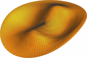
Away from resonance, the free surface is gently sloping and is only slightly deformed. For resonant cases, as shown in figures 4 and 5, the wave profile has two peaks in the middle, and there exists a saddle-shaped depression between the two crests (at the centre of the circular basin). This phenomenon is caused by the second-harmonic resonant wave component (2,2), which is significant for resonant cases since it has a similar amplitude to that of the fundamental wave component (1,1).

Figure 4. Wave profiles for $d=0.831377$ at $t=0$: (a) $\epsilon =0.9997$, (b) $\epsilon =0.9989$.

Figure 5. Wave profile for $d=0.831377$ and $\epsilon =1.00014$ at $t=0$.

Wave profiles for (1,2)-TW with $\epsilon =0.9997$ and $\epsilon =0.9989$ are shown in figure 4. Here $\epsilon =0.9997$ corresponds to a case with weak nonlinearity, while $\epsilon =0.9989$ corresponds to a case with a stronger nonlinearity. When $\epsilon =0.9997$, the free surface of the (1,2)-TW is smooth. However, when $\epsilon =0.9989$, there are more ripples on the surface of the wave, that are due to the influence of higher-order harmonic wave components. The profiles for (1,2)-TW with $\epsilon =1.00014$ are shown in figure 5. The wave profiles are similar to those with $\epsilon <1$, but there are some differences. Comparing the conditions with $\epsilon =0.9989$ and $\epsilon =1.00014$ at $t=0$, one sees that the orientation of the waveforms is different. It illustrates that $\epsilon <1$ and $\epsilon >1$ are associated with two different (1,2)-TW. Furthermore, since the coefficient of the resonant wave component (2,2) is approximately $1.7$ times the coefficient of the fundamental wave component (1,1) for the case with $\epsilon =1.00014$, in contrast to the case with $\epsilon =0.9989$, the second-harmonic resonant wave component plays a more important role in the entire wave. The two peaks are more prominent, and the area of the two protrusions is relatively large.

4. (1,2)-SW

The same resonance can be found for SW in a circular basin. For SW, the governing equation and boundary conditions are (2.1)–(2.5) without the dependence on $\theta$. In addition, we have the condition of mass conservation:

(4.1)\begin{equation} \int_{0}^{1}r\eta_s(r,t)\,\textrm{d}r=0. \end{equation}

The linear solutions of the standing-wave system read

(4.2)\begin{gather} \bar{\eta}_s(r,t)=a^s \textrm{J}_0(k_{j}r) \cos i(\omega_s t), \end{gather}

(4.3)\begin{gather} \bar{\varphi}_s(r,z,t)=b^s \textrm{J}_0(k_{j}r)\frac{\cosh k_{j}(z+d)}{\cosh k_{j}d} \sin i(\omega_s t), \end{gather}

where $k_{j}$ denotes the $j$th zero of $\textrm {J}'_0$:

(4.4)\begin{equation} \textrm{J}'_0(k_{j})=0\quad (i=1,2,\ldots,\ j=1,2,\ldots). \end{equation}

The linear solution satisfies the dispersion relation

(4.5)\begin{equation} i^2\omega_s^2=k_{j}\tanh\, k_{j}d . \end{equation}

For nonlinear waves dominated by the fundamental wave component (1,1) (i.e. $i=j=1$), the linear frequency is

(4.6)\begin{equation} \omega_s^2=k_{1}{{\tanh}}\,k_{1}d. \end{equation}

Due to nonlinear interactions, higher-order harmonic wave components can be generated. Under certain conditions, the harmonic wave component ($i, j$) will resonate with the fundamental wave component ($1, 1$). Resonance occurs at ratios of depth to radius $d$ such that there exists a $k_{j}$ satisfying

(4.7)\begin{equation} i(k_{1}{{\tanh}}\,k_{1}d)^{1/2}=(k_{j}{{\tanh}}\,k_{j}d)^{1/2}. \end{equation}

There exist different sets of resonant wave components associated with each one of the ratios of depth to radius, as shown in table 6. The case $i=2, j=3$ corresponds to the second-harmonic resonance studied in the present paper.

Table 6. Ratios of depth to radius $d$ satisfying the linear resonance relation for standing waves (Mack Reference Mack1962).

Similarly, due to the nonlinearity, the actual wave frequency $\sigma _s$ is slightly different from the linear frequency $\omega _s=\sqrt {k_{1}{{\tanh }}\,k_{1}d}$, and also depends on the wave amplitude. Let $\epsilon _s={\sigma }_s/{ \omega }_s$. Then, we define the variable

(4.8)\begin{equation} \xi_s= \sigma_s t. \end{equation}

Like for TW, we solve the standing-wave problem in a new coordinate system ($r$, $z$, $\xi _s$). The standing-wave elevation $\eta (r, \xi _s)$ and the velocity potential $\varphi (r, z, \xi _s)$ can be described by combinations of the linear solution (4.2) and (4.3):

(4.9)\begin{gather} \eta_s= \sum_{i=0}^\infty \sum_{j=1}^\infty a^s_{ij} \textrm{J}_0(k_{j}r) \cos i\xi_s, \end{gather}

(4.10)\begin{gather} \varphi_s=\sum_{i=1}^\infty \sum_{j=1}^\infty b^s_{ij} \varPsi^s_{ij}, \end{gather}

with

(4.11)\begin{equation} \varPsi^s_{ij} (r,\xi, z)=\textrm{J}_0(k_{j}r)\frac{\cosh k_{j}(z+d)}{\cosh k_{j}d} \sin i\xi_s, \end{equation}

where $a^s_{ij}$ and $b^s_{ij}$ are constants to be determined later. Note that the velocity potential (4.10) satisfies the linear governing equation, the boundary conditions on $r=1$ and $r=-d$ and the wave elevation (4.9) satisfies the condition of mass conservation (4.1) identically. Therefore, the unknown coefficients $a^s_{ij}$ and $b^s_{ij}$ are determined by the two nonlinear boundary conditions on the free surface.

Like for TW, we have the so-called homotopy-series solutions for resonant SW in a circular basin for the unknown velocity potential $\varphi _s$ and free-surface elevation $\eta _s$. They read

(4.12)\begin{gather} \varphi_s (r, z, \xi_s)=\sum_{m=0}^{+\infty }\varphi^s _m(r, z, \xi_s), \end{gather}

(4.13)\begin{gather} \eta_s (r, \xi_s)=\sum_{m=0}^{+\infty }\eta^s _m(r, \xi_s). \end{gather}

As opposed to the steady-state (1,2)-TW in a circular basin, we take the nonlinear frequency $\sigma _s$ as an unknown quantity. The so-called homotopy-series solution about the nonlinear frequency $\sigma _s$ is

(4.14)\begin{equation} \sigma_s=\sum_{m=0}^{+\infty }\sigma^s _{m}. \end{equation}

The calculations are similar to those for (1,2)-TW in a circular basin. It is worth noting that we choose the initial guess of the velocity potential $\varphi _s$ as

(4.15)\begin{equation} \varphi^s _0=B^s_{11}\varPsi^s_{11}+B^s_{23,0}\varPsi^s_{23}, \end{equation}

where the constant $B^s_{11}$ is given and corresponds to the primary wave. The unknown constants $\sigma ^s_{0}$ and $B^s_{23,0}$ are determined by avoiding the secular terms $\textrm {J}_0(k_{1}r) \sin \xi _s$ and $\textrm {J}_0(k_{3}r) \sin 2\xi _s$ appearing on the right-hand side of the first-order deformation equation. The rest of the calculation process is similar to that of the (1,2)-TW in a circular basin.

We consider the second-harmonic resonance of nonlinear SW dominated by the fundamental wave component (1,1) with ratios of depth to radius $d=0.198143$. The corresponding resonant wave mode is the (2,3) mode. With the HAM-based analytical approach, we successfully obtain (1,2)-SW in a circular basin. The converged results with different values of $B^s_{11}$ in the initial guess of the velocity potential are listed in table 7. It is found that, when resonance occurs, the amplitude of the fundamental wave component (1,1) and of the resonant wave component (2,3) are of the same order of magnitude. As the value of $B_{11}^s$ decreases, the nonlinearity of the (1,2)-SW shows an increasing trend. The amplitude coefficients in front of the fundamental wave component (1,1) and the resonant wave component (2,3) both increase. According to the variation of the value of $B_{11}^s$, we found two branches of convergent solutions for the (1,2)-SW in a circular basin, that correspond to the cases $a^s_{2,3}/a^s_{1,1}>0$ and $a^s_{2,3}/a^s_{1,1}<0$ respectively. Figure 6 shows the value of $\epsilon _s=\sigma _s/\omega _s$ as a function of $B_{11}^s$. The two branches of (1,2)-SW split when the value of $B_{11}^s$ approaches $0$. As the value of $B_{11}^s$ decreases, the set of solutions $a^s_{2,3}/a^s_{1,1}>0$ goes further.

Figure 6. Value of $\epsilon _s=\sigma _s/\omega _s$ as a function of $B_{11}^s$ for (1,2)-SW.

Table 7. (1,2)-SW: dimensionless frequency $\epsilon _s$, wave amplitude components and $H=|\eta _s(0,0)-\eta _s(1,0)|$ for $d=0.198143$ with different values of $B^s_{11}$ in the initial guess of the velocity potential.

5. Concluding remarks and discussion

The water-wave equations in a circular cylinder with nonlinear boundary conditions on the free surface are solved by a coupled analytical and numerical approach to obtain second-harmonic resonant waves with time-independent spectra. For nonlinear TW dominated by the fundamental wave component (1,1) in a circular basin, the second-harmonic wave component (2,2) resonates with the fundamental wave component (1,1) when the ratio of water depth to radius $d=0.831377$. For nonlinear SW dominated by the fundamental wave component (1,1), the (2,3) mode resonates with the fundamental wave component (1,1) when the ratio of water depth to radius $d=0.198143$.

In the resonance problem considered here, the second-harmonic resonant wave component corresponds to a mathematical singularity, which is difficult to deal with in the framework of perturbation methods. Additionally, the convergence rate of the series solution obtained from the HAM reduces as the nonlinearity increases. The slow convergence rate of series solutions obtained from the HAM makes it impossible to consider steady-state resonant waves with strong nonlinearity. To overcome these difficulties, a solution procedure that combines the HAM-based analytical approach and a Galerkin numerical-method-based approach has been used. Based on the HAM, when the resonance occurs, only the resonant wave component needs to be added in the initial guess, and the secular term thus generated can be successfully avoided. Then, an approximate homotopy-series solution to the steady second-harmonic resonant waves can be obtained. The Galerkin numerical method-based approach is used to obtain accurate steady-state solutions. In this way, we successfully obtained steady nonlinear second-harmonic resonant waves in a circular basin. However, even the numerical method shows some slow convergence and high accuracy is difficult to reach for large nonlinearities. It will be interesting to use in future work numerical methods that do not rely on Bessel functions. The algorithm recently proposed by Qadeer & Wilkening (Reference Qadeer and Wilkening2019) looks promising.

This paper confirms the existence of finite-amplitude steady-state (1,2)-TW and (1,2)-SW in a circular basin. There are two branches of (1,2)-TW solutions, one with dimensionless angular frequency slightly less than one ($\epsilon <1$) and one with dimensionless angular frequency slightly more than one ($\epsilon >1$). The coefficients of the fundamental wave component (1,1) and of the second-harmonic resonant wave component (2,2) are much larger than the other wave components, which means that most of the wave energy resides in the fundamental and second-harmonic resonant wave components. Based on our results, the amplitude of the wave group increases continuously with the nonlinearity of the wave. As the nonlinearity increases (the value of $|\epsilon -1|$ becomes larger), an increasing number of higher-order harmonics play a role in the whole wave. In addition, the (1,2)-resonance also exists in the case of SW in a circular basin. Similarly, there are two branches of steady-state (1,2)-SW in a circular basin.

The results in the present paper deepen our understanding of the resonance of gravity waves in a circular basin, which may occur in harbours or bays. We conclude with two suggestions for future work. Bridges (Reference Bridges1990) showed that in addition to well-known TW and SW other classes of periodic waves, in particular three-mode MW, may exist. It will be interesting to check whether such MW can be computed with the method used in the present paper. The branches of TW and SW have different behaviours. It will be interesting to use state-of-the-art numerical methods to follow the branches towards more extreme waves.