


1 Introduction
Falling liquid films have received much attention from researchers in recent decades (Chang Reference Chang1994; Oron, Davis & Bankoff Reference Oron, Davis and Bankoff1997; Weinstein & Ruschak Reference Weinstein and Ruschak2004; Craster & Matar Reference Craster and Matar2009; Ruyer-Quil et al. Reference Ruyer-Quil, Kofman, Chasseur and Mergui2014). As examples of open-flow systems, they are encountered in many industrial fields, like coating processes (Alekseenko, Nakoryakov & Pokusaev Reference Alekseenko, Nakoryakov and Pokusaev1994), heat exchangers (Salvagnini & Taqueda Reference Salvagnini and Taqueda2004), cooling microelectronic devices (Squires & Quake Reference Squires and Quake2005), chemical reactors (Bender, Stephan & Gambaryan-Roisman Reference Bender, Stephan and Gambaryan-Roisman2017), food processing and thermal protection design of combustion chambers in rocket engines (Shine & Nidhi Reference Shine and Nidhi2018). Investigation of this subject was pioneered by the experimental work of Kapitza & Kapitza (Reference Kapitza and Kapitza1949). Theoretical studies were later carried out by Benjamin (Reference Benjamin1957) and Yih (Reference Yih1963), where the threshold value of Reynolds number when the film is unstable with long-wave perturbations was shown to depend on the inclination angle. Alekseenko, Nakoryakov & Pokusaev (Reference Alekseenko, Nakoryakov and Pokusaev1985) experimentally measured the growth rate of the waves and compared that with theoretical results. Smith (Reference Smith1990) carefully scrutinized the mechanism of this long-wave instability and concluded that the inertial stress associated with the Reynolds number is the key factor that destabilizes the film. Later, Liu, Paul & Gollub (Reference Liu, Paul and Gollub1993) conducted decisive experiments and confirmed the theoretical predictions of the critical Reynolds number of Benjamin (Reference Benjamin1957) and Yih (Reference Yih1963). Over the years, experimental efforts have been made continually to validate and complement the theoretical studies on falling films (Liu, Schneider & Gollub Reference Liu, Schneider and Gollub1995; Alekseenko et al. Reference Alekseenko, Antipin, Guzanov, Kharlamov and Markovich2005; Kharlamov et al. Reference Kharlamov, Guzanov, Bobylev, Alekseenko and Markovich2015; Adebayo et al. Reference Adebayo, Xie, Che and Matar2017; Charogiannis et al. Reference Charogiannis, Denner, van Wachem, Kalliadasis and Markides2017; Charogiannis & Markides Reference Charogiannis and Markides2019).
Since the full treatment of the Navier–Stokes equations together with boundary conditions on the free surface and solid bottom remains a cumbersome task, many efforts have been made to seek a simplified model based on the long-wave nature of the film instability. Benney (Reference Benney1966) first devised a single evolution equation of the film thickness  $h$ using an expansion method in a small film parameter. Following this procedure, a number of researches have been performed that showed its effectiveness in the prediction of the instability threshold (Lin Reference Lin1974; Joo, Davis & Bankoff Reference Joo, Davis and Bankoff1991; Sadiq & Usha Reference Sadiq and Usha2008; Samanta Reference Samanta2008; Ogden, Pascal & D’Alessio Reference Ogden, Pascal and D’Alessio2011; Dávalos-Orozco Reference Dávalos-Orozco2012). However, several authors have pointed out that the Benney-type equation blows up and yields unphysical solutions at moderate Reynolds numbers (Pumir, Manneville & Pomeau Reference Pumir, Manneville and Pomeau1983; Scheid et al. Reference Scheid, Ruyer-Quil, Thiele, Kabov, Legros and Colinet2005). On the other hand, an integral-boundary-layer (IBL) model was first developed by Shkadov (Reference Shkadov1967) which couples the film thickness
  $h$ and local flow rate
  $q$. Then, a weighted residual technique was proposed which is able to remove the inconsistency between the original IBL model and the full Navier–Stokes equations in determining the instability threshold (Ruyer-Quil & Manneville Reference Ruyer-Quil and Manneville2000, Reference Ruyer-Quil and Manneville2002). After that, this method has been adopted to model the film flow in many other situations (Trevelyan et al. Reference Trevelyan, Scheid, Ruyer-Quil and Kalliadasis2007; Samanta, Ruyer-Quil & Goyeau Reference Samanta, Ruyer-Quil and Goyeau2011; Amaouche, Djema & Ait Abderrahmane Reference Amaouche, Djema and Ait Abderrahmane2012; Ruyer-Quil, Chakraborty & Dandapat Reference Ruyer-Quil, Chakraborty and Dandapat2012; Ding & Wong Reference Ding and Wong2015; D’Alessio & Pascal Reference D’Alessio and Pascal2016; Ellaban, Pascal & D’Alessio Reference Ellaban, Pascal and D’Alessio2017; Fu, Hu & Yang Reference Fu, Hu and Yang2018).
Surfactants could be used to induce a variation in surface tension (known as Marangoni effect or surface elasticity) and surface viscosity, which can thus adjust the surface dynamics (Scriven & Sternling Reference Scriven and Sternling1960). The influence of insoluble surfactants on a falling film was first studied theoretically by Benjamin (Reference Benjamin1964) and Whitaker (Reference Whitaker1964). They both found an increase of the critical Reynolds number when surface elasticity is included, concluding that there was a stabilizing effect of surfactants, which was qualitatively in accordance with several earlier experimental observations (Emmert Reference Emmert1954; Stirba & Hurt Reference Stirba and Hurt1955; Tailby & Portalski Reference Tailby and Portalski1961). Blyth & Pozrikidis (Reference Blyth and Pozrikidis2004) identified a new Marangoni mode when surfactants are present and concluded that there was a stabilizing effect of surfactants overall. Using a perturbation expansion method, Oron & Edwards (Reference Oron and Edwards1993) derived a nonlinear evolution equation for the free-surface displacement of the film in the presence of interfacial viscous stress. Pereira & Kalliadasis (Reference Pereira and Kalliadasis2008) considered the problem in both linear and nonlinear regimes. They solved the Orr–Sommerfeld eigenvalue problem of the full equations and obtained three different modes in linear instability, where they stated that the Marangoni stress caused by surfactants reduces the domain of film instability. On the basis of the weighted residual model (WRM), they also found that the amplitude and velocity of travelling waves on the film are decreased by the Marangoni effect. Ji & Setterwall (Reference Ji and Setterwall1994) studied the case where surfactants are soluble and volatile, which they claimed is necessary to destabilize the Marangoni mode.
Karapetsas & Bontozoglou (Reference Karapetsas and Bontozoglou2014) focused on the influence of arbitrary solubility of the surfactants and found that the interfacial concentration gradient decreases with increasing surfactant solubility; higher-order calculations showed that the speed of adsorption/desorption at the interface plays a role at finite wavelength. Meanwhile, experiments were also carried out where an attenuation influence of soluble surfactants on inlet disturbances were observed (Georgantaki, Vlachogiannis & Bontozoglou Reference Georgantaki, Vlachogiannis and Bontozoglou2012, Reference Georgantaki, Vlachogiannis and Bontozoglou2016). In some recent relative research, Bhat & Samanta (Reference Bhat and Samanta2018) considered a falling film down a slippery plane in the presence of insoluble surfactants and showed that insoluble surfactants stabilize the shear mode at high Reynolds number. Also, they found that when the Péclet number exceeds its critical value, the surfactant mode becomes unstable, while the inertia force does not affect the surfactant mode significantly (Bhat & Samanta Reference Bhat and Samanta2019). Pascal, D’Alessio & Ellaban (Reference Pascal, D’Alessio and Ellaban2019) developed a model accounting for the transport of surfactants between the surface and the bulk of the film layer where the variation of the fluid density was also incorporated. Their results depict a non-monotonic relation between the critical Reynolds number and the variation of density.
In this paper we study the effect of insoluble surfactants on a falling film when both surface elasticity and surface viscosities are taken into account, which has not been clearly clarified in the literature up to now. Next, § 2 gives the governing equations of the film flow and derives a WRM which accounts for the effects of both surface elasticity and surface viscosities. In § 3, we examine the linear stability characteristics and compare the results of full equations and the WRM. Travelling wave solutions are discussed in § 4, and finally we summarize the main conclusions in § 5.
2 Problem formulation
2.1 Governing equations
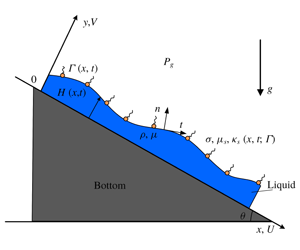
We consider a two-dimensional incompressible liquid film flowing down an inclined plane. As depicted in figure 1, the interface between the film and the ambient gas is covered with insoluble surfactants. A Cartesian coordinate system  $(x,y)$ is established so that the
  $x$ axis is parallel to the solid bottom and points in the downstream direction while
  $y$ is normal to the bottom and points outwards. The density, viscosity and surface tension of the fluid are
  $\unicode[STIX]{x1D70C}$,
  $\unicode[STIX]{x1D707}$ and
  $\unicode[STIX]{x1D70E}$, respectively,
  $g$ is the gravitational acceleration and
  $\unicode[STIX]{x1D703}$ denotes the inclination angle.

Figure 1. Schematic of a thin falling film covered with insoluble surfactants.
In the film layer, we have the continuity and Navier–Stokes equations:
 $$\begin{eqnarray}\displaystyle & \displaystyle \frac{\unicode[STIX]{x2202}U}{\unicode[STIX]{x2202}x}+\frac{\unicode[STIX]{x2202}V}{\unicode[STIX]{x2202}y}=0, & \displaystyle\end{eqnarray}$$
 $$\begin{eqnarray}\displaystyle & \displaystyle \unicode[STIX]{x1D70C}\left(\frac{\unicode[STIX]{x2202}U}{\unicode[STIX]{x2202}t}+U\frac{\unicode[STIX]{x2202}U}{\unicode[STIX]{x2202}x}+V\frac{\unicode[STIX]{x2202}U}{\unicode[STIX]{x2202}y}\right)=-\frac{\unicode[STIX]{x2202}P}{\unicode[STIX]{x2202}x}+\unicode[STIX]{x1D707}\left(\frac{\unicode[STIX]{x2202}^{2}U}{\unicode[STIX]{x2202}x^{2}}+\frac{\unicode[STIX]{x2202}^{2}U}{\unicode[STIX]{x2202}y^{2}}\right)+\unicode[STIX]{x1D70C}g\sin \unicode[STIX]{x1D703}, & \displaystyle\end{eqnarray}$$
 $$\begin{eqnarray}\displaystyle & \displaystyle \unicode[STIX]{x1D70C}\left(\frac{\unicode[STIX]{x2202}V}{\unicode[STIX]{x2202}t}+U\frac{\unicode[STIX]{x2202}V}{\unicode[STIX]{x2202}x}+V\frac{\unicode[STIX]{x2202}V}{\unicode[STIX]{x2202}y}\right)=-\frac{\unicode[STIX]{x2202}P}{\unicode[STIX]{x2202}y}+\unicode[STIX]{x1D707}\left(\frac{\unicode[STIX]{x2202}^{2}V}{\unicode[STIX]{x2202}x^{2}}+\frac{\unicode[STIX]{x2202}^{2}V}{\unicode[STIX]{x2202}y^{2}}\right)-\unicode[STIX]{x1D70C}g\cos \unicode[STIX]{x1D703}, & \displaystyle\end{eqnarray}$$
 where  $U$ and
  $V$ are velocity components in the
  $x$ and
  $y$ directions, respectively, and
  $P$ is the pressure. Introducing
  $F_{1}=1+(\unicode[STIX]{x2202}H/\unicode[STIX]{x2202}x)^{2}$ and
  $F_{2}=1-(\unicode[STIX]{x2202}H/\unicode[STIX]{x2202}x)^{2}$, the concentration
  $\unicode[STIX]{x1D6E4}$ of the insoluble surfactants obeys the following transport equation at the interface
  $y=H(x,t)$ (Pereira & Kalliadasis Reference Pereira and Kalliadasis2008):
 $$\begin{eqnarray}\frac{\unicode[STIX]{x2202}\unicode[STIX]{x1D6E4}}{\unicode[STIX]{x2202}t}+U\frac{\unicode[STIX]{x2202}\unicode[STIX]{x1D6E4}}{\unicode[STIX]{x2202}x}+\frac{\unicode[STIX]{x1D6E4}}{F_{1}}\left[\left(\frac{\unicode[STIX]{x2202}U}{\unicode[STIX]{x2202}x}+\frac{\unicode[STIX]{x2202}H}{\unicode[STIX]{x2202}x}\frac{\unicode[STIX]{x2202}V}{\unicode[STIX]{x2202}x}\right)+\frac{\unicode[STIX]{x2202}H}{\unicode[STIX]{x2202}x}\left(\frac{\unicode[STIX]{x2202}U}{\unicode[STIX]{x2202}y}+\frac{\unicode[STIX]{x2202}H}{\unicode[STIX]{x2202}x}\frac{\unicode[STIX]{x2202}V}{\unicode[STIX]{x2202}y}\right)\right]=\frac{D_{s}}{\sqrt{F_{1}}}\frac{\unicode[STIX]{x2202}}{\unicode[STIX]{x2202}x}\left(\frac{1}{\sqrt{F_{1}}}\frac{\unicode[STIX]{x2202}\unicode[STIX]{x1D6E4}}{\unicode[STIX]{x2202}x}\right).\end{eqnarray}$$
 Here the first two terms on the left-hand side of (2.4) denote the material derivative of  $\unicode[STIX]{x1D6E4}$; while the third term represents the change of the concentration resulting from the stretching of the surface. The term on the right-hand side accounts for the diffusion of surfactants on the surface, with
  $D_{s}$ being the surface diffusivity. At the solid bottom
  $y=0$, the non-slip boundary condition requires
 $$\begin{eqnarray}U=V=0.\end{eqnarray}$$
 The kinematic condition at the free surface  $y=H(x,t)$ is
 $$\begin{eqnarray}V=\frac{\unicode[STIX]{x2202}H}{\unicode[STIX]{x2202}t}+U\frac{\unicode[STIX]{x2202}H}{\unicode[STIX]{x2202}x}.\end{eqnarray}$$
 In the present formulation, we consider the case where the surfactant induces both surface elasticity and viscosities on the free surface. Namely, it not only reduces the surface tension but also induces extra viscous stresses at the interface, as described by Martínez-Calvo & Sevilla (Reference Martínez-Calvo and Sevilla2018), where the free-surface stresses are modelled by two surface viscosities: the surface shear viscosity  $\unicode[STIX]{x1D707}_{s}(\unicode[STIX]{x1D6E4})$ and dilatational viscosity
  $\unicode[STIX]{x1D705}_{s}(\unicode[STIX]{x1D6E4})$. Following their procedure, we introduce
  $\boldsymbol{U}_{s}=U_{n}\,\boldsymbol{n}+U_{t}\,\boldsymbol{t}$ to denote the film velocity at the surface with
 $$\begin{eqnarray}\displaystyle \left\{\begin{array}{@{}l@{}}\displaystyle \boldsymbol{n}=\frac{1}{\sqrt{F_{1}}}\left(-\frac{\unicode[STIX]{x2202}H}{\unicode[STIX]{x2202}x},1\right),\\ \displaystyle \boldsymbol{t}=\frac{1}{\sqrt{F_{1}}}\left(1,\frac{\unicode[STIX]{x2202}H}{\unicode[STIX]{x2202}x}\right),\end{array}\right.\quad \text{and}\quad \left\{\begin{array}{@{}l@{}}\displaystyle U_{n}=\frac{1}{\sqrt{F_{1}}}\left(V-\frac{\unicode[STIX]{x2202}H}{\unicode[STIX]{x2202}x}U\right),\\ \displaystyle U_{t}=\frac{1}{\sqrt{F_{1}}}\left(U+\frac{\unicode[STIX]{x2202}H}{\unicode[STIX]{x2202}x}V\right)\end{array}\right. & & \displaystyle\end{eqnarray}$$
 being the unit normal and tangential vectors and the corresponding velocity components at the surface. If we let  $\unicode[STIX]{x1D64F}$ and
  $\unicode[STIX]{x1D64F}_{g}$ be the stress tensors of the fluid and the surrounding gas, respectively, the surface equation of motion is given by (Martínez-Calvo & Sevilla Reference Martínez-Calvo and Sevilla2018)
 $$\begin{eqnarray}\displaystyle & & \displaystyle (\unicode[STIX]{x1D64F}_{g}-\unicode[STIX]{x1D64F})\boldsymbol{\cdot }\boldsymbol{n}+\unicode[STIX]{x1D735}_{s}\unicode[STIX]{x1D70E}-\boldsymbol{n}\boldsymbol{\cdot }(\unicode[STIX]{x1D735}_{s}\boldsymbol{\cdot }\boldsymbol{n})\unicode[STIX]{x1D70E}+\unicode[STIX]{x1D735}_{s}[(\unicode[STIX]{x1D705}_{s}-\unicode[STIX]{x1D707}_{s})(\unicode[STIX]{x1D735}_{s}\boldsymbol{\cdot }\boldsymbol{U}_{s})]\nonumber\\ \displaystyle & & \displaystyle \quad -\boldsymbol{n}\boldsymbol{\cdot }(\unicode[STIX]{x1D735}_{s}\boldsymbol{\cdot }\boldsymbol{n})(\unicode[STIX]{x1D705}_{s}-\unicode[STIX]{x1D707}_{s})(\unicode[STIX]{x1D735}_{s}\boldsymbol{\cdot }\boldsymbol{U}_{s})+\unicode[STIX]{x1D735}_{s}\boldsymbol{\cdot }\{\unicode[STIX]{x1D707}_{s}[(\unicode[STIX]{x1D735}_{s}\boldsymbol{U}_{s})\boldsymbol{\cdot }\unicode[STIX]{x1D644}_{s}+\unicode[STIX]{x1D644}_{s}\boldsymbol{\cdot }(\unicode[STIX]{x1D735}_{s}\boldsymbol{U}_{s})^{\text{T}}]\}=0,\end{eqnarray}$$
 where  $\unicode[STIX]{x1D644}_{s}=\unicode[STIX]{x1D644}-\boldsymbol{n}\boldsymbol{n}$ is the surface projection operator and
  $\unicode[STIX]{x1D735}_{s}=\unicode[STIX]{x1D644}_{s}\boldsymbol{\cdot }\unicode[STIX]{x1D735}$ is the surface gradient operator, with
  $\unicode[STIX]{x1D644}$ being the identity tensor. Note that the pressure of the surrounding gas is assumed to be constant and thus
  $\unicode[STIX]{x1D64F}_{g}=-P_{g}\unicode[STIX]{x1D644}$. Evaluating the inner product of (2.8) with
  $\boldsymbol{n}$ and
  $\boldsymbol{t}$, we obtain two dynamical boundary conditions at
  $y=H(x,t)$:
 $$\begin{eqnarray}\displaystyle & & \displaystyle (P-P_{g})-\frac{2\unicode[STIX]{x1D707}}{F_{1}}\left[\frac{\unicode[STIX]{x2202}V}{\unicode[STIX]{x2202}y}+\left(\frac{\unicode[STIX]{x2202}H}{\unicode[STIX]{x2202}x}\right)^{2}\frac{\unicode[STIX]{x2202}U}{\unicode[STIX]{x2202}x}-\frac{\unicode[STIX]{x2202}H}{\unicode[STIX]{x2202}x}\left(\frac{\unicode[STIX]{x2202}U}{\unicode[STIX]{x2202}y}+\frac{\unicode[STIX]{x2202}V}{\unicode[STIX]{x2202}x}\right)\right]\nonumber\\ \displaystyle & & \displaystyle \quad =-\frac{\unicode[STIX]{x2202}^{2}H}{\unicode[STIX]{x2202}x^{2}}\left[\frac{\unicode[STIX]{x1D70E}}{{F_{1}}^{3/2}}+\frac{1}{{F_{1}}^{2}}(\unicode[STIX]{x1D707}_{s}+\unicode[STIX]{x1D705}_{s})\left(\frac{\unicode[STIX]{x2202}U_{t}}{\unicode[STIX]{x2202}x}-\frac{\unicode[STIX]{x2202}^{2}H}{\unicode[STIX]{x2202}x^{2}}\frac{U_{n}}{F_{1}}\right)\right]\end{eqnarray}$$
and
 $$\begin{eqnarray}\displaystyle & & \displaystyle \frac{\unicode[STIX]{x1D707}}{\sqrt{F_{1}}}\left[\left(\frac{\unicode[STIX]{x2202}U}{\unicode[STIX]{x2202}y}+\frac{\unicode[STIX]{x2202}V}{\unicode[STIX]{x2202}x}\right)F_{2}+2\frac{\unicode[STIX]{x2202}H}{\unicode[STIX]{x2202}x}\left(\frac{\unicode[STIX]{x2202}V}{\unicode[STIX]{x2202}y}-\frac{\unicode[STIX]{x2202}U}{\unicode[STIX]{x2202}x}\right)\right]\nonumber\\ \displaystyle & & \displaystyle \quad =\frac{\unicode[STIX]{x2202}\unicode[STIX]{x1D70E}}{\unicode[STIX]{x2202}x}+\frac{\unicode[STIX]{x2202}}{\unicode[STIX]{x2202}x}\left[(\unicode[STIX]{x1D707}_{s}+\unicode[STIX]{x1D705}_{s})\left(\frac{1}{\sqrt{F_{1}}}\frac{\unicode[STIX]{x2202}U_{t}}{\unicode[STIX]{x2202}x}-\frac{U_{n}}{{F_{1}}^{3/2}}\frac{\unicode[STIX]{x2202}^{2}H}{\unicode[STIX]{x2202}x^{2}}\right)\right].\end{eqnarray}$$
 Here, as noted by Martínez-Calvo & Sevilla (Reference Martínez-Calvo and Sevilla2018), the velocity components  $U$ and
  $V$ in
  $U_{t}$ and
  $U_{n}$ are interface quantities, which are previously evaluated at the free surface. Considering this fact, for example, the derivative of
  $U$ with respect to
  $x$ at the interface is
 $$\begin{eqnarray}\frac{\unicode[STIX]{x2202}U(x,y=H(x,t),t)}{\unicode[STIX]{x2202}x}=\left.\frac{\unicode[STIX]{x2202}U}{\unicode[STIX]{x2202}x}\right|_{y=H(x,t)}+\frac{\unicode[STIX]{x2202}H}{\unicode[STIX]{x2202}x}\left.\frac{\unicode[STIX]{x2202}U}{\unicode[STIX]{x2202}y}\right|_{y=H(x,t)}.\end{eqnarray}$$
 It is obvious that the two surface viscosities are indistinguishable from each other and act like a single parameter; thus we introduce  $\unicode[STIX]{x1D6FD}=\unicode[STIX]{x1D707}_{s}+\unicode[STIX]{x1D705}_{s}$ to denote the overall effect of surface viscosities for simplicity. Moreover, according to Ponce-Torres et al. (Reference Ponce-Torres, Montanero, Herrada, Vega and Vega2017), the surface viscosities depend on the concentration and can be expressed as
  $\unicode[STIX]{x1D6FD}(\unicode[STIX]{x1D6E4})=\unicode[STIX]{x1D6FD}^{\ast }\unicode[STIX]{x1D6E4}$, with
  $\unicode[STIX]{x1D6FD}^{\ast }$ being a surfactant constant. Besides, the surface elasticity represents the surface tension gradient caused by surfactants with the relation
  $\unicode[STIX]{x1D70E}(\unicode[STIX]{x1D6E4})=\unicode[STIX]{x1D70E}_{0}-\unicode[STIX]{x1D6FE}(\unicode[STIX]{x1D6E4}-\unicode[STIX]{x1D6E4}_{0})$ (
 $\unicode[STIX]{x1D6FE}$ being positive here).
We now apply the following scaling procedure to the above equations:
 $$\begin{eqnarray}\left.\begin{array}{@{}c@{}}\displaystyle x=l\,\overline{x},\quad y=H_{N}\overline{y},\quad U=U_{0}\overline{u},\quad V=\unicode[STIX]{x1D6FF}U_{0}\overline{v},\quad H=H_{N}\overline{h},\\ \displaystyle t=\frac{l}{U_{0}}\overline{t},\quad \unicode[STIX]{x1D6E4}=\unicode[STIX]{x1D6E4}_{0}\overline{\unicode[STIX]{x1D719}},\quad P-P_{g}=\unicode[STIX]{x1D70C}U_{0}^{2}\overline{p}.\end{array}\right\}\end{eqnarray}$$
 Here  $H_{N}$ is the Nusselt thickness given by
 $$\begin{eqnarray}H_{N}=\left(\frac{3\unicode[STIX]{x1D707}Q}{\unicode[STIX]{x1D70C}g\sin \unicode[STIX]{x1D703}}\right)^{1/3},\end{eqnarray}$$
 where  $Q$ is the flow rate, and
  $U_{0}=Q/H_{N}$ is the average velocity of the basic flow. Note that in (2.12) a thin-film parameter
  $\unicode[STIX]{x1D6FF}=H_{N}/l$ is formulated and
  $\unicode[STIX]{x1D6FF}\ll 1$ is considered a small number. After implementing the non-dimensionalization and dropping the bar on the dimensionless variables for convenience, the governing equations (2.1)–(2.10) become
 $$\begin{eqnarray}\displaystyle & \displaystyle \frac{\unicode[STIX]{x2202}u}{\unicode[STIX]{x2202}x}+\frac{\unicode[STIX]{x2202}v}{\unicode[STIX]{x2202}y}=0, & \displaystyle\end{eqnarray}$$
 $$\begin{eqnarray}\displaystyle & \displaystyle \unicode[STIX]{x1D6FF}Re\left(\frac{\unicode[STIX]{x2202}u}{\unicode[STIX]{x2202}t}+u\frac{\unicode[STIX]{x2202}u}{\unicode[STIX]{x2202}x}+v\frac{\unicode[STIX]{x2202}u}{\unicode[STIX]{x2202}y}\right)=-\unicode[STIX]{x1D6FF}Re\frac{\unicode[STIX]{x2202}p}{\unicode[STIX]{x2202}x}+3+\unicode[STIX]{x1D6FF}^{2}\frac{\unicode[STIX]{x2202}^{2}u}{\unicode[STIX]{x2202}x^{2}}+\frac{\unicode[STIX]{x2202}^{2}u}{\unicode[STIX]{x2202}y^{2}}, & \displaystyle\end{eqnarray}$$
 $$\begin{eqnarray}\displaystyle & \displaystyle \unicode[STIX]{x1D6FF}^{2}Re\left(\frac{\unicode[STIX]{x2202}v}{\unicode[STIX]{x2202}t}+u\frac{\unicode[STIX]{x2202}v}{\unicode[STIX]{x2202}x}+v\frac{\unicode[STIX]{x2202}v}{\unicode[STIX]{x2202}y}\right)=-Re\frac{\unicode[STIX]{x2202}p}{\unicode[STIX]{x2202}y}-3\cot \unicode[STIX]{x1D703}+\unicode[STIX]{x1D6FF}^{3}\frac{\unicode[STIX]{x2202}^{2}v}{\unicode[STIX]{x2202}x^{2}}+\unicode[STIX]{x1D6FF}\frac{\unicode[STIX]{x2202}^{2}v}{\unicode[STIX]{x2202}y^{2}}, & \displaystyle\end{eqnarray}$$
 $$\begin{eqnarray}\displaystyle & & \displaystyle \frac{\unicode[STIX]{x2202}\unicode[STIX]{x1D719}}{\unicode[STIX]{x2202}t}+u\frac{\unicode[STIX]{x2202}\unicode[STIX]{x1D719}}{\unicode[STIX]{x2202}x}+\frac{\unicode[STIX]{x1D719}}{f_{1}}\left[\left(\frac{\unicode[STIX]{x2202}u}{\unicode[STIX]{x2202}x}+\unicode[STIX]{x1D6FF}^{2}\frac{\unicode[STIX]{x2202}h}{\unicode[STIX]{x2202}x}\frac{\unicode[STIX]{x2202}v}{\unicode[STIX]{x2202}x}\right)+\frac{\unicode[STIX]{x2202}h}{\unicode[STIX]{x2202}x}\left(\frac{\unicode[STIX]{x2202}u}{\unicode[STIX]{x2202}y}+\unicode[STIX]{x1D6FF}^{2}\frac{\unicode[STIX]{x2202}h}{\unicode[STIX]{x2202}x}\frac{\unicode[STIX]{x2202}v}{\unicode[STIX]{x2202}y}\right)\right]\nonumber\\ \displaystyle & & \displaystyle \quad =\frac{\unicode[STIX]{x1D6FF}}{Pe_{s}\sqrt{f_{1}}}\frac{\unicode[STIX]{x2202}}{\unicode[STIX]{x2202}x}\left(\frac{1}{\sqrt{f_{1}}}\frac{\unicode[STIX]{x2202}\unicode[STIX]{x1D719}}{\unicode[STIX]{x2202}x}\right),\end{eqnarray}$$
 where  $Re=\unicode[STIX]{x1D70C}U_{0}H_{N}/\unicode[STIX]{x1D707}$ is the Reynolds number and
  $Pe_{s}=U_{0}H_{N}/D_{s}$ is the surface Péclet number.
The dimensionless non-slip condition at  $y=0$ is
 $$\begin{eqnarray}u=v=0,\end{eqnarray}$$
 while the kinematic condition at  $y=h(x,t)$ can be written as
 $$\begin{eqnarray}v=\frac{\unicode[STIX]{x2202}h}{\unicode[STIX]{x2202}t}+u\frac{\unicode[STIX]{x2202}h}{\unicode[STIX]{x2202}x}.\end{eqnarray}$$
The dynamic boundary conditions (2.9)–(2.10) are transformed to
 $$\begin{eqnarray}\displaystyle & & \displaystyle p-\frac{2\unicode[STIX]{x1D6FF}}{Ref_{1}}\left[\frac{\unicode[STIX]{x2202}v}{\unicode[STIX]{x2202}y}+\unicode[STIX]{x1D6FF}^{2}\left(\frac{\unicode[STIX]{x2202}h}{\unicode[STIX]{x2202}x}\right)^{2}\frac{\unicode[STIX]{x2202}u}{\unicode[STIX]{x2202}x}-\frac{\unicode[STIX]{x2202}h}{\unicode[STIX]{x2202}x}\left(\frac{\unicode[STIX]{x2202}u}{\unicode[STIX]{x2202}y}+\unicode[STIX]{x1D6FF}^{2}\frac{\unicode[STIX]{x2202}v}{\unicode[STIX]{x2202}x}\right)\right]\nonumber\\ \displaystyle & & \displaystyle \quad =-\frac{\unicode[STIX]{x1D6FF}}{Re}\frac{\unicode[STIX]{x2202}^{2}h}{\unicode[STIX]{x2202}x^{2}}\left[\frac{3\unicode[STIX]{x1D6FF}[We-Ma(\unicode[STIX]{x1D719}-1)]}{{f_{1}}^{3/2}}+\frac{\unicode[STIX]{x1D6FF}^{2}Bo}{{f_{1}}^{2}}\unicode[STIX]{x1D719}\left(\frac{\unicode[STIX]{x2202}u_{t}}{\unicode[STIX]{x2202}x}-\unicode[STIX]{x1D6FF}\frac{\unicode[STIX]{x2202}^{2}h}{\unicode[STIX]{x2202}x^{2}}\frac{u_{n}}{f_{1}}\right)\right]\end{eqnarray}$$
and
 $$\begin{eqnarray}\displaystyle & & \displaystyle \frac{1}{\sqrt{f_{1}}}\left[\left(\frac{\unicode[STIX]{x2202}u}{\unicode[STIX]{x2202}y}+\frac{\unicode[STIX]{x2202}v}{\unicode[STIX]{x2202}x}\right)f_{2}+2\unicode[STIX]{x1D6FF}^{2}\frac{\unicode[STIX]{x2202}h}{\unicode[STIX]{x2202}x}\left(\frac{\unicode[STIX]{x2202}v}{\unicode[STIX]{x2202}y}-\frac{\unicode[STIX]{x2202}u}{\unicode[STIX]{x2202}x}\right)\right]\nonumber\\ \displaystyle & & \displaystyle \quad =-3\unicode[STIX]{x1D6FF}Ma\frac{\unicode[STIX]{x2202}\unicode[STIX]{x1D719}}{\unicode[STIX]{x2202}x}+\unicode[STIX]{x1D6FF}^{2}Bo\frac{\unicode[STIX]{x2202}}{\unicode[STIX]{x2202}x}\left[\unicode[STIX]{x1D719}\left(\frac{1}{\sqrt{f_{1}}}\frac{\unicode[STIX]{x2202}u_{t}}{\unicode[STIX]{x2202}x}-\frac{\unicode[STIX]{x1D6FF}u_{n}}{{f_{1}}^{3/2}}\frac{\unicode[STIX]{x2202}^{2}h}{\unicode[STIX]{x2202}x^{2}}\right)\right],\end{eqnarray}$$
 where  $We=\unicode[STIX]{x1D70E}_{0}/\unicode[STIX]{x1D70C}gH_{N}^{2}\sin \unicode[STIX]{x1D703}$ is the Weber number,
  $Ma=\unicode[STIX]{x1D6FE}\unicode[STIX]{x1D6E4}_{0}/\unicode[STIX]{x1D70C}gH_{N}^{2}\sin \unicode[STIX]{x1D703}$ denotes the Marangoni number and
  $Bo=\unicode[STIX]{x1D6FD}^{\ast }\unicode[STIX]{x1D6E4}_{0}/\unicode[STIX]{x1D707}H_{N}$ is the Boussinesq number. The other variables are given by
 $$\begin{eqnarray}\displaystyle u_{n}=\frac{\unicode[STIX]{x1D6FF}}{\sqrt{f_{1}}}\left(v-\frac{\unicode[STIX]{x2202}h}{\unicode[STIX]{x2202}x}u\right)\quad \text{and}\quad u_{t}=\frac{1}{\sqrt{f_{1}}}\left(u+\frac{\unicode[STIX]{x2202}h}{\unicode[STIX]{x2202}x}v\right), & & \displaystyle\end{eqnarray}$$
where
 $$\begin{eqnarray}\displaystyle f_{1}=1+\unicode[STIX]{x1D6FF}^{2}\left(\frac{\unicode[STIX]{x2202}h}{\unicode[STIX]{x2202}x}\right)^{2}\quad \text{and}\quad f_{2}=1-\unicode[STIX]{x1D6FF}^{2}\left(\frac{\unicode[STIX]{x2202}h}{\unicode[STIX]{x2202}x}\right)^{2}. & & \displaystyle\end{eqnarray}$$
2.2 Weighted residual model
Now we employ the WRM to derive a set of reduced equations that incorporates the effect of insoluble surfactants. As done in previous works (Ogden et al. Reference Ogden, Pascal and D’Alessio2011; D’Alessio & Pascal Reference D’Alessio and Pascal2016; Ellaban et al. Reference Ellaban, Pascal and D’Alessio2017; Fu et al. Reference Fu, Hu and Yang2018), we discard terms of orders higher than  $O(\unicode[STIX]{x1D6FF}^{2})$ in (2.14)–(2.21) and begin by assuming a profile of the velocity
 $$\begin{eqnarray}u=\frac{3q}{2h^{3}}b_{1}+\frac{\unicode[STIX]{x1D6FF}Ma}{4h}b_{2}\frac{\unicode[STIX]{x2202}\unicode[STIX]{x1D719}}{\unicode[STIX]{x2202}x},\end{eqnarray}$$
 where  $b_{1}=y(2h-y)$,
  $b_{2}=y(2h-3y)$ and
  $q=\int _{0}^{h}u\,\text{d}y$ is the flow rate. Note that the prescribed velocity
  $u$ satisfies the non-slip condition (2.18) and the tangential stress condition (2.21) to the first order in
  $\unicode[STIX]{x1D6FF}$:
 $$\begin{eqnarray}\left.\frac{\unicode[STIX]{x2202}u}{\unicode[STIX]{x2202}y}\right|_{y=h}=-3\unicode[STIX]{x1D6FF}Ma\frac{\unicode[STIX]{x2202}\unicode[STIX]{x1D719}}{\unicode[STIX]{x2202}x}.\end{eqnarray}$$
 Given (2.24), we can readily obtain the velocity  $v$ through (2.14) and (2.18). First, equation (2.16) is integrated from
  $y=h$ to
  $y$, combining with the condition (2.20), which yields
 $$\begin{eqnarray}p=\frac{3\cot \unicode[STIX]{x1D703}}{Re}(h-y)-\frac{\unicode[STIX]{x1D6FF}}{Re}\left.\!\frac{\unicode[STIX]{x2202}u}{\unicode[STIX]{x2202}x}\right|_{h}-\frac{\unicode[STIX]{x1D6FF}}{Re}\frac{\unicode[STIX]{x2202}u}{\unicode[STIX]{x2202}x}-\frac{3\unicode[STIX]{x1D6FF}^{2}}{Re}[We-Ma(\unicode[STIX]{x1D719}-1)]\frac{\unicode[STIX]{x2202}^{2}h}{\unicode[STIX]{x2202}x^{2}}.\end{eqnarray}$$
 Equation (2.26) can be used to eliminate the pressure in (2.15) with terms of  $O(\unicode[STIX]{x1D6FF}^{2})$ being dropped since
  $p$ is multiplied with
  $\unicode[STIX]{x1D6FF}$ in (2.15); while
  $We$ is assumed to be of
  $O(1/\unicode[STIX]{x1D6FF})$ or larger to retain the effect of surface tension. Integrating (2.14) over the film thickness and applying the conditions (2.18) and (2.19), one arrives at
 $$\begin{eqnarray}\frac{\unicode[STIX]{x2202}h}{\unicode[STIX]{x2202}t}+\frac{\unicode[STIX]{x2202}q}{\unicode[STIX]{x2202}x}=0.\end{eqnarray}$$
 Here, in accordance with the idea of the Galerkin method, we choose  $b_{1}$ as the weighted function and multiply it with (2.15), then integrate from
  $y=0$ to
  $y=h$ and utilize (2.21). Moreover, substituting
  $u$ and
  $v$ into (2.17) and collecting terms up to
  $O(\unicode[STIX]{x1D6FF}^{2})$, we finally obtain the following equations for
  $h$,
$h$,  $q$ and
  $\unicode[STIX]{x1D719}$:
 $$\begin{eqnarray}\displaystyle & & \displaystyle \frac{\unicode[STIX]{x2202}q}{\unicode[STIX]{x2202}t}+\frac{\unicode[STIX]{x2202}}{\unicode[STIX]{x2202}x}\left(\frac{9q^{2}}{7h}+\frac{5\cot \unicode[STIX]{x1D703}}{4Re}h^{2}+\frac{15Ma}{4Re}\unicode[STIX]{x1D719}\right)\nonumber\\ \displaystyle & & \displaystyle \quad =\frac{q}{7h}\frac{\unicode[STIX]{x2202}q}{\unicode[STIX]{x2202}x}+\frac{5}{2\unicode[STIX]{x1D6FF}Re}\left(h-\frac{q}{h^{2}}\right)+\frac{5\unicode[STIX]{x1D6FF}^{2}We}{2Re}h\frac{\unicode[STIX]{x2202}^{3}h}{\unicode[STIX]{x2202}x^{3}}\nonumber\\ \displaystyle & & \displaystyle \qquad -\,\frac{15\unicode[STIX]{x1D6FF}Bo}{8Reh^{2}}\left[\unicode[STIX]{x1D719}\frac{\unicode[STIX]{x2202}}{\unicode[STIX]{x2202}x}\left(q\frac{\unicode[STIX]{x2202}h}{\unicode[STIX]{x2202}x}\right)-h\frac{\unicode[STIX]{x2202}}{\unicode[STIX]{x2202}x}\left(\unicode[STIX]{x1D719}\frac{\unicode[STIX]{x2202}q}{\unicode[STIX]{x2202}x}\right)+\frac{\unicode[STIX]{x2202}h}{\unicode[STIX]{x2202}x}\frac{\unicode[STIX]{x2202}}{\unicode[STIX]{x2202}x}\left(q\unicode[STIX]{x1D719}\right)-\frac{2q\unicode[STIX]{x1D719}}{h}\left(\frac{\unicode[STIX]{x2202}h}{\unicode[STIX]{x2202}x}\right)^{2}\right]\nonumber\\ \displaystyle & & \displaystyle \qquad +\,\frac{\unicode[STIX]{x1D6FF}Ma}{16}\left[h^{2}\frac{\unicode[STIX]{x2202}^{2}\unicode[STIX]{x1D719}}{\unicode[STIX]{x2202}x\unicode[STIX]{x2202}t}+\frac{45}{14}hq\frac{\unicode[STIX]{x2202}^{2}\unicode[STIX]{x1D719}}{\unicode[STIX]{x2202}x^{2}}+\frac{19h}{7}\frac{\unicode[STIX]{x2202}q}{\unicode[STIX]{x2202}x}\frac{\unicode[STIX]{x2202}\unicode[STIX]{x1D719}}{\unicode[STIX]{x2202}x}+\frac{15q}{7}\frac{\unicode[STIX]{x2202}h}{\unicode[STIX]{x2202}x}\frac{\unicode[STIX]{x2202}\unicode[STIX]{x1D719}}{\unicode[STIX]{x2202}x}\right]\nonumber\\ \displaystyle & & \displaystyle \qquad +\,\frac{\unicode[STIX]{x1D6FF}}{Re}\left[\frac{9}{2}\frac{\unicode[STIX]{x2202}^{2}q}{\unicode[STIX]{x2202}x^{2}}-\frac{9}{2h}\frac{\unicode[STIX]{x2202}q}{\unicode[STIX]{x2202}x}\frac{\unicode[STIX]{x2202}h}{\unicode[STIX]{x2202}x}+\frac{4q}{h^{2}}\left(\frac{\unicode[STIX]{x2202}h}{\unicode[STIX]{x2202}x}\right)^{2}-\frac{6q}{h}\frac{\unicode[STIX]{x2202}^{2}h}{\unicode[STIX]{x2202}x^{2}}\right],\end{eqnarray}$$
 $$\begin{eqnarray}\displaystyle \frac{\unicode[STIX]{x2202}\unicode[STIX]{x1D719}}{\unicode[STIX]{x2202}t}+\frac{\unicode[STIX]{x2202}}{\unicode[STIX]{x2202}x}\left(\frac{3q\unicode[STIX]{x1D719}}{2h}\right) & = & \displaystyle \frac{\unicode[STIX]{x1D6FF}}{Pe_{s}}\frac{\unicode[STIX]{x2202}^{2}\unicode[STIX]{x1D719}}{\unicode[STIX]{x2202}x^{2}}+\frac{3\unicode[STIX]{x1D6FF}Mah}{4}\left[\left(\frac{\unicode[STIX]{x2202}\unicode[STIX]{x1D719}}{\unicode[STIX]{x2202}x}\right)^{2}+\unicode[STIX]{x1D719}\frac{\unicode[STIX]{x2202}^{2}\unicode[STIX]{x1D719}}{\unicode[STIX]{x2202}x^{2}}\right]\nonumber\\ \displaystyle & & \displaystyle +\,\frac{3\unicode[STIX]{x1D6FF}Ma\unicode[STIX]{x1D719}}{4}\frac{\unicode[STIX]{x2202}h}{\unicode[STIX]{x2202}x}\frac{\unicode[STIX]{x2202}\unicode[STIX]{x1D719}}{\unicode[STIX]{x2202}x}-\unicode[STIX]{x1D6FF}^{2}\left(\frac{3q}{2h}\frac{\unicode[STIX]{x2202}^{2}h}{\unicode[STIX]{x2202}x^{2}}-\frac{\unicode[STIX]{x2202}^{2}q}{\unicode[STIX]{x2202}x^{2}}\right)\frac{\unicode[STIX]{x2202}h}{\unicode[STIX]{x2202}x}\unicode[STIX]{x1D719}.\end{eqnarray}$$
 Equations (2.27)–(2.29) constitute a second-order WRM for a falling film with both surface elasticity and surface viscosities induced by the insoluble surfactants on the free surface. In deriving (2.27)–(2.29), it is assumed that the parameters  $Re$,
$Re$,  $Ma$,
$Ma$,  $Bo$,
$Bo$,  $Pe_{s}$ and
  $\cot \unicode[STIX]{x1D703}$ are of
  $O(1)$. By setting
  $Bo=0$, dropping the second-order terms and using the same scaling, equations (2.27)–(2.29) can recover the first-order weighted IBL equations of Pereira & Kalliadasis (Reference Pereira and Kalliadasis2008) where only the surface elasticity is considered.
3 Linear stability analysis
To study the linear stability of the film, we impose small disturbances on the basic flow, which can be expressed in the form of a normal mode:
 $$\begin{eqnarray}(h,q,\unicode[STIX]{x1D719})=(h_{s},q_{s},\unicode[STIX]{x1D719}_{s})+({\hat{h}},\hat{q},\hat{\unicode[STIX]{x1D719}})\exp (\text{i}kx+\unicode[STIX]{x1D714}t)+\text{c.c.},\end{eqnarray}$$
where c.c. represents the complex conjugate of the second term. Substituting (3.1) into (2.27)–(2.29) and linearizing the equations, a dispersion relation is obtained as follows:
 $$\begin{eqnarray}\left|\begin{array}{@{}ccc@{}}D_{11} & D_{12} & D_{13}\\ D_{21} & D_{22} & D_{23}\\ D_{31} & D_{32} & D_{33}\end{array}\right|=0,\end{eqnarray}$$
 where  $D_{11}{-}D_{33}$ are given by
 $$\begin{eqnarray}\displaystyle \left.\begin{array}{@{}c@{}}\displaystyle D_{11}=\unicode[STIX]{x1D714},\quad D_{12}=\text{i}k,\quad D_{13}=0,\\ \displaystyle D_{21}=\frac{-420+140\text{i}We\unicode[STIX]{x1D6FF}^{3}k^{3}-21(5Bo+16)\unicode[STIX]{x1D6FF}^{2}k^{2}-4\text{i}(18Re-35\cot \unicode[STIX]{x1D703})\unicode[STIX]{x1D6FF}k}{56\unicode[STIX]{x1D6FF}Re},\\ \displaystyle D_{22}=\frac{140+21(5Bo+12)\unicode[STIX]{x1D6FF}^{2}k^{2}+8(17\text{i}k+7\unicode[STIX]{x1D714})\unicode[STIX]{x1D6FF}Re}{56\unicode[STIX]{x1D6FF}Re},\\ \displaystyle D_{23}=\frac{Mak}{16Re}\left[60\text{i}-\left(\text{i}\unicode[STIX]{x1D714}-\frac{45}{14}k\right)\unicode[STIX]{x1D6FF}\mathit{Re}\right],\quad D_{31}=-\frac{3}{2}\text{i}k,\quad D_{32}=\frac{3}{2}\text{i}k,\\ \displaystyle D_{33}=\unicode[STIX]{x1D714}+\frac{3}{2}\text{i}k+\frac{3Ma\unicode[STIX]{x1D6FF}k^{2}}{4}+\frac{\unicode[STIX]{x1D6FF}k^{2}}{Pe_{s}}.\end{array}\right\} & & \displaystyle\end{eqnarray}$$
 After assuming  $\unicode[STIX]{x1D714}=\unicode[STIX]{x1D714}_{r}+\text{i}\unicode[STIX]{x1D714}_{i}$ and setting the temporal growth rate
  $\unicode[STIX]{x1D714}_{r}=0$ in (3.2), we can obtain the neutral stability cases, where one can finally determine the critical Reynolds number as
 $$\begin{eqnarray}Re_{c}={\textstyle \frac{5}{6}}\cot \unicode[STIX]{x1D703}+{\textstyle \frac{5}{2}}Ma.\end{eqnarray}$$
Here we note that, as long as the same scaling is adopted, equation (3.4) agrees with the result of Pereira & Kalliadasis (Reference Pereira and Kalliadasis2008) where only the effect of surface elasticity is considered, which means that surface elasticity increases the critical Reynolds number while the existence of surface viscosity actually does not affect the instability threshold.
Meanwhile, we also solve the linear stability based on full equations (2.14)–(2.21). After linearization and assuming the disturbances of the variables in (2.14)–(2.21) to be
 $$\begin{eqnarray}(u^{\prime },v^{\prime },p^{\prime },\unicode[STIX]{x1D719}^{\prime },h^{\prime })=(\hat{u} ,\hat{v},\hat{p},\hat{\unicode[STIX]{x1D719}},{\hat{h}})\exp (\text{i}kx+\unicode[STIX]{x1D714}t)+\text{c.c.},\end{eqnarray}$$
 the system is actually reduced to an ordinary differential equation eigenvalue problem, with  $\unicode[STIX]{x1D714}$ being the eigenvalue. A Chebyshev spectral collocation method is employed to solve this problem, which is a well-known technique to study hydrodynamic stability (Khorrami, Malik & Ash Reference Khorrami, Malik and Ash1989). Applying the Chebyshev spectral collocation method and upon discretization, the problem is then converted to a generalized eigenvalue problem
 $$\begin{eqnarray}\unicode[STIX]{x1D63C}\,\boldsymbol{s}=\unicode[STIX]{x1D714}\unicode[STIX]{x1D63D}\,\boldsymbol{s},\end{eqnarray}$$
 where  $\unicode[STIX]{x1D63C}$ and
  $\unicode[STIX]{x1D63D}$ are square matrices, with
  $\boldsymbol{s}$ being a column vector that contains the values of
  $\hat{u}$,
  $\hat{v}$,
  $\hat{p}$,
  $\hat{\unicode[STIX]{x1D719}}$ and
  ${\hat{h}}$ at the collocation points. The computer program is based on a universal software package which has been developed by the authors to analyse hydrodynamic stability problems (Ye, Yang & Fu Reference Ye, Yang and Fu2016).
Note that in experiments it is generally convenient to control the film thickness or the Reynolds number through the flow rate. Hence we introduce a set of flow parameters that only depend on the physical properties:
 $$\begin{eqnarray}\displaystyle Ka=\frac{\unicode[STIX]{x1D70E}_{0}}{\unicode[STIX]{x1D70C}g^{1/3}\unicode[STIX]{x1D710}^{4/3}},\quad M=\frac{\unicode[STIX]{x1D6FE}\unicode[STIX]{x1D6E4}_{0}}{\unicode[STIX]{x1D70C}g^{1/3}\unicode[STIX]{x1D710}^{4/3}},\quad Sc=\frac{\unicode[STIX]{x1D710}}{D_{s}},\quad Bo_{0}=\frac{\unicode[STIX]{x1D6FD}^{\ast }\unicode[STIX]{x1D6E4}_{0}}{\unicode[STIX]{x1D70C}g^{-1/3}\unicode[STIX]{x1D710}^{5/3}}, & & \displaystyle\end{eqnarray}$$
 where  $Ka$ is the Kapitza number,
  $M$ is a modified Marangoni number representing the magnitude of the surface elasticity,
  $Sc$ is the Schmidt number and
  $Bo_{0}$ corresponds to the modified Boussinesq number characterizing the effect of surface viscosities, with
  $\unicode[STIX]{x1D710}=\unicode[STIX]{x1D707}/\unicode[STIX]{x1D70C}$ denoting the kinematic viscosity of the fluid. Given
  $\unicode[STIX]{x1D712}=gH_{N}^{3}/\unicode[STIX]{x1D710}^{2}$ as the modified Reynolds number, equations (3.7) are related to previous parameters by
 $$\begin{eqnarray}\displaystyle Re=\frac{\unicode[STIX]{x1D712}}{3}\sin \unicode[STIX]{x1D703},\quad We=\frac{Ka}{\unicode[STIX]{x1D712}^{2/3}\sin \unicode[STIX]{x1D703}},\quad Ma=\frac{M}{\unicode[STIX]{x1D712}^{2/3}\sin \unicode[STIX]{x1D703}},\quad Pe_{s}=\frac{\unicode[STIX]{x1D712}}{3}Sc\sin \unicode[STIX]{x1D703},\quad Bo=\frac{Bo_{0}}{\unicode[STIX]{x1D712}^{1/3}}. & & \displaystyle \nonumber\\ \displaystyle & & \displaystyle\end{eqnarray}$$
 Figure 2 depicts the three least stable modes in the linear regime. Following the notation of Pereira & Kalliadasis (Reference Pereira and Kalliadasis2008), they belong to the Kapitza mode due to classical long-wave instability, the concentration mode due to the diffusion and advection of surface species, and the shear mode due to the velocity profile, respectively. It is obvious that the growth rates of the concentration mode and shear mode are negative and are thus stable modes, while the Kapitza mode is unstable for small wavenumber; note that the shear mode could be unstable at some finite wavenumber when  $\unicode[STIX]{x1D712}$ is very large (Pereira & Kalliadasis Reference Pereira and Kalliadasis2008). Moreover, the surface viscosities show a stabilizing effect on the Kapitza mode and shear mode while they slightly increase the growth rate of the concentration mode which still remains stable. Here we shall mainly focus on the Kapitza mode in the following parts since it is the only unstable mode in the long-wave region.

Figure 2. Growth rates of the three least stable modes calculated from the full equations when  $\unicode[STIX]{x1D712}=15$ and
  $M=1$. The solid, dashed and dot-dashed lines correspond to the Kapitza, concentration and shear modes, respectively. Two different values of modified Boussinesq numbers are presented:
  $Bo_{0}=0$ for thick lines and
  $Bo_{0}=20$ for thin lines. Other parameters are
  $\unicode[STIX]{x1D703}=\unicode[STIX]{x03C0}/2$,
  $Ka=3376$ and
  $Sc=100$, which are fixed in the present study.

Figure 3. Effect of surface elasticity on the linear stability when  $Bo_{0}=10$: (a) temporal growth rate and wave speed when
  $\unicode[STIX]{x1D712}=15$, and (b) neutral stability curves. The solid, dashed and dot-dashed lines correspond to three modified Marangoni numbers 0, 3 and 6. Thick and thin lines represent the results of full equations and WRM, respectively (the same notation is adopted in figure 4).
Figure 3 displays the influence of the surface elasticity on the film instability. Clearly, as the modified Marangoni number increases, both the growth rate and the cutoff wavenumber decrease remarkably while the wave speed increases at the same time. Moreover, as shown in figure 3(b), one can see that the instability threshold becomes larger and the unstable region diminishes when  $M$ increases, which shows a stabilizing effect of the surface elasticity on the film. In fact, a larger modified Marangoni number leads to stronger surface elasticity, which means the surface tension is more sensitive to the change of the surfactant concentration. Given the expression in (3.1) or (3.5), the small disturbances of film thickness
  $h$ and surfactant concentration
  $\unicode[STIX]{x1D719}$ are in phase, which means the value of surface tension is out of phase with the film thickness in the case
  $M>0$ considered here. This results in a larger value of surface tension in the troughs and a smaller value in the crests, which tends to drive the fluid flowing from the crests to the troughs, thus dampening the surface undulation and stabilizing the film.

Figure 4. Effect of surface viscosities on the linear stability when  $M=3$: (a) temporal growth rate and wave speed when
  $\unicode[STIX]{x1D712}=15$, and (b) neutral stability curves. The solid, dashed and dot-dashed lines correspond to three modified Boussinesq numbers 0, 10 and 20.
The influence of surface viscosities is depicted in figure 4. It can be seen that the temporal growth rate, cutoff wavenumber and wave speed decrease as  $Bo_{0}$ becomes larger, which implies that surface viscosities basically act to stabilize the film. However, as shown in figure 4(b), though the unstable region becomes smaller when
  $Bo_{0}$ increases, the instability threshold remains the same, which is in accordance with (3.4). Furthermore, unlike the surface elasticity, the effect of surface viscosities gradually decreases as
  $k\rightarrow 0$ or
  $Re\rightarrow Re_{c}$, showing almost no impact in the long-wave limit, which also supports the result that the instability threshold is not altered when the surface viscosities come into play. From figure 4 we can see that the impact of surface viscosities here is similar to that of the bulk viscosity, which attenuates the linear waves and enhances the dispersion effect, especially for wavenumbers close to the neutral value. Note that in figures 3 and 4, the results of the WRM nicely coincide with those of the full equations.
4 Travelling wave solutions
It has been observed in experiments that small initial disturbances generally evolve into travelling waves on the free surface, which propagate at a constant speed  $c$ and wave shape (Alekseenko et al. Reference Alekseenko, Nakoryakov and Pokusaev1985; Liu, Gollub & Aarts Reference Liu, Gollub and Aarts1994). In this section, we will make an effort to determine the travelling wave solutions based on the model equations (2.27)–(2.29). First we apply a coordinate transformation
  $\unicode[STIX]{x1D709}=x-ct$, so that (2.27) becomes
 $$\begin{eqnarray}-ch^{\prime }+q^{\prime }=0,\end{eqnarray}$$
 where a prime represents the derivative with respect to  $\unicode[STIX]{x1D709}$. Integrating (4.1) leads to
  $q=ch+q_{0}$ with
  $q_{0}$ being an integral constant. Substituting this into (2.28) and (2.29) and implementing the transformation, we have
 $$\begin{eqnarray}\displaystyle & \displaystyle A_{1}h^{\prime \prime \prime }+A_{2}h^{\prime \prime }+A_{3}\unicode[STIX]{x1D719}^{\prime \prime }+A_{4}{h^{\prime }}^{2}+A_{5}h^{\prime }\unicode[STIX]{x1D719}^{\prime }+A_{6}h^{\prime }+A_{7}\unicode[STIX]{x1D719}^{\prime }+A_{8}=0, & \displaystyle\end{eqnarray}$$
 $$\begin{eqnarray}\displaystyle & \displaystyle B_{1}\unicode[STIX]{x1D719}^{\prime \prime }+B_{2}h^{\prime \prime }+B_{3}{\unicode[STIX]{x1D719}^{\prime }}^{2}+B_{4}\unicode[STIX]{x1D719}^{\prime }+B_{5}\unicode[STIX]{x1D719}=0, & \displaystyle\end{eqnarray}$$
 where expressions for  $A_{1}{-}A_{8}$ and
  $B_{1}{-}B_{5}$ are given in appendix A. A closed flow condition is imposed,
 $$\begin{eqnarray}\frac{1}{L}\int _{0}^{L}h\,\text{d}\unicode[STIX]{x1D709}=1,\end{eqnarray}$$
 where  $L=2\unicode[STIX]{x03C0}/k$ is the wavelength, and a phase condition,
  $h(0)=\unicode[STIX]{x1D719}(0)=1$, is applied. After discretization by the Fourier spectral method, equations (4.2) and (4.3) are converted into a nonlinear algebra system, with
  $k$ being a parameter. We solve this problem by the Newton–Kantorovich method together with the continuation method. An initial guess of the wave speed and profiles could be obtained from the neutral stability solutions.

Figure 5. (a) The speed of the travelling wave and (b) the difference between the maximum and minimum amplitudes as functions of normalized wavenumber  $k/k_{n}$ at different modified Marangoni numbers when
  $Bo_{0}=10$ and
  $\unicode[STIX]{x1D712}=15$. Solid, dashed and dot-dashed lines are for
  $M=0$,
  $M=3$ and
  $M=6$.
Presented in figure 5 is the effect of the surface elasticity on the bifurcation diagram. The fast-wave family  $\unicode[STIX]{x1D6FE}_{2}$ emerges from the trivial solution at the cutoff wavenumber
  $k_{n}$ through a Hopf bifurcation. The slow-wave family
  $\unicode[STIX]{x1D6FE}_{1}$ originates from the
  $\unicode[STIX]{x1D6FE}_{2}$ family through a period-doubling bifurcation. This bifurcation diagram is not altered when surface elasticity exists. We can see that, as the modified Marangoni number
  $M$ increases, the wave speed gradually approaches that of the linear kinematic waves; and the gap
  $\unicode[STIX]{x0394}h_{m}=h_{max}-h_{min}$ between the maximum and minimum amplitudes is significantly reduced. Specifically, on the
  $\unicode[STIX]{x1D6FE}_{2}$ branches the speed decreases remarkably when
  $k/k_{n}<0.5$, while it slightly increases when
  $k/k_{n}>0.6$ with
  $M$. In other words, the surface elasticity decelerates the fast-wave family, while it accelerates the slow-wave family, thus weakening the dispersion effect. This is consistent with the result of linear stability analysis in figure 3, where the Marangoni effect is shown to promote the speed of linear waves and attenuate the dispersion of the system.
Figure 6 displays the corresponding profiles of fast  $\unicode[STIX]{x1D6FE}_{2}$ waves and slow
  $\unicode[STIX]{x1D6FE}_{1}$ waves of figure 5. The fast waves consist of one hump following a series of small capillary waves; the slow waves are made of one trough preceding the capillary waves. The wave shape of the surfactant concentration
  $\unicode[STIX]{x1D719}$ is similar to that of the film thickness
  $h$ while its amplitude is obviously larger. For fast waves, the amplitudes of both humps and capillary ripples are dampened markedly as the surface elasticity becomes stronger. Consequently, the height of the flat portion of travelling waves is promoted due to the conservation of mass. A similar suppressing effect on the troughs and capillary waves is also observed for slow waves. Physically, the surface elasticity acts like a restoring force which resists the deformation of the free surface from the basic state.

Figure 6. Wave profiles of film thickness  $h$ and surfactant concentration
  $\unicode[STIX]{x1D719}$: (a) fast
  $\unicode[STIX]{x1D6FE}_{2}$ family and (b) slow
  $\unicode[STIX]{x1D6FE}_{1}$ family. Solid, dashed and dot-dashed lines are for
  $M=0$,
  $M=3$ and
  $M=6$. The wavenumber is chosen to be
  $k=0.02$.
We now explore the effect of surface elasticity on the  $\unicode[STIX]{x1D6FE}_{2}$ wave, since only the one-hump wave could be obtained during the simulation (Pumir et al. Reference Pumir, Manneville and Pomeau1983). From figure 7 we can observe that, as the modified Reynolds number increases, both the wave speed and the maximum amplitude are promoted, showing the destabilizing effect of the inertia, which also implies that waves with large amplitude travel faster than those with small amplitude. For a given
  $\unicode[STIX]{x1D712}$, both the maximum amplitude and the wave speed are reduced when the surface elasticity becomes stronger, again manifesting its stabilizing impact on the film flow.

Figure 7. Variation of properties of  $\unicode[STIX]{x1D6FE}_{2}$ waves with modified Reynolds number
  $\unicode[STIX]{x1D712}$: (a) speed
  $c$, and (b) maximum amplitude
  $h_{max}$ when
  $Bo_{0}=10$ and
  $k=0.02$. Solid, dashed and dot-dashed lines are for
  $M=0$,
  $M=3$ and
  $M=6$.
The influence of the surface viscosities on the bifurcation diagram is demonstrated in figure 8. First we notice that the surface viscosities can modify the bifurcation behaviour of the system. Specifically, in figure 8(c,d), when  $Bo_{0}$ is relatively large, the bifurcation diagram is similar to that in figure 5; whereas the opposite situation happens when the surface viscosity effect is very weak, as shown in figure 8(a,b), which is also the case when surface viscosities are absent (
 $Bo_{0}=0$). Similar modification of the bifurcation diagram was also identified for the effect of bulk viscous diffusion (Scheid, Ruyer-Quil & Manneville Reference Scheid, Ruyer-Quil and Manneville2006). In both cases, for
  $k/k_{n}<0.5$ (waves with typical humps or troughs), surface viscosities slightly promote the speed
  $c$ and the amplitude gap
  $\unicode[STIX]{x0394}h_{m}$ of the fast
  $\unicode[STIX]{x1D6FE}_{2}$ waves; as for slow
  $\unicode[STIX]{x1D6FE}_{1}$ waves, increasing the value of
  $Bo_{0}$ leads to a minor increase of the wave speed with a small reduction of the amplitude gap. When
  $k/k_{n}>0.6$, the surface viscosity effect tends to decrease the wave speed and dampen the amplitude gap. Thus, we may say that surface viscosities have exerted some additional dispersion effect in the system.
Similarly, we present the wave profiles for different values of  $Bo_{0}$ in figure 9. It can be seen that, for fast waves, the surface viscosity effect dampens the capillary ripples while it augments the height of the humps. On the other hand, it decreases the amplitude of troughs and amplifies that of the capillary ripples for slow waves. In fact, figures 6 and 9 both show that
  $\unicode[STIX]{x1D6FE}_{2}$ waves with steeper humps travel faster while
  $\unicode[STIX]{x1D6FE}_{1}$ waves with shallower troughs propagate at a lower speed.

Figure 8. Effect of the surface viscosities on the bifurcation diagram when  $M=3$ and
  $\unicode[STIX]{x1D712}=15$: (a,c) speed of the travelling waves, and (b,d) difference between maximum and minimum amplitudes.

Figure 9. Wave profiles of film thickness  $h$ and surfactant concentration
  $\unicode[STIX]{x1D719}$: (a) fast
  $\unicode[STIX]{x1D6FE}_{2}$ family and (b) slow
  $\unicode[STIX]{x1D6FE}_{1}$ family at different modified Boussinesq numbers. The wavenumber is chosen to be
  $k=0.02$.
5 Conclusions
We investigate the effect of insoluble surfactants on the stability of a thin film falling down an inclined plate and consider the case where surfactants induce both elasticity and viscosities on the free surface. The tangential and normal stress conditions are derived on the two-dimensional free surface of the film under the current Cartesian coordinate system. Both surface elasticity and viscosities are assumed to vary with the concentration of surfactants in a linear relation. The weighted residual method (WRM) is adopted to obtain a reduced model to study the film instability. In the linear analysis, it is found that the surface elasticity remarkably decreases the temporal growth rate and increases the instability threshold, showing a stabilizing role on the film instability; and though the surface viscosity effect does not modify the critical Reynolds number, it decreases the growth rate and cutoff wavenumber. The results of the WRM agree with those of the full equations satisfactorily. Travelling wave solutions are obtained from the reduced model. Surface elasticity reduces the speed of the fast-wave family while it increases that of the slow-wave family, thus damping the dispersion effect. And it suppresses the amplitude of both large-amplitude humps (troughs) and small-amplitude capillary waves, causing an effect to resist the deformation of the free surface. On the other hand, the surface viscosity effect can modify the bifurcation diagram. Moreover, it acts to slightly increase the amplitude of the fast-wave family, decrease that of the slow-wave family and promote the wave speed of both families when the wavelengths are relatively large. Overall, surface viscosities tend to damp the linear waves, modify the bifurcation diagram and add some dispersion effect to the system, which is somewhat similar to the role of bulk viscosity.
Acknowledgements
We are grateful to the referees for their instructive comments and suggestions that improved the manuscript. This work was supported by the China’s National Natural Science Funds for Distinguished Young Scholar (grant no. 11525207) and China’s National Natural Science Foundation (grant nos. 11272036 and 11672025).
Declaration of interests
The authors report no conflict of interest.
Appendix A. Coefficients of the governing equations in a moving frame
 $$\begin{eqnarray}\displaystyle \left.\begin{array}{@{}c@{}}\displaystyle A_{1}=-\frac{5}{2Re}\unicode[STIX]{x1D6FF}^{2}Weh,\quad A_{2}=\frac{3\unicode[STIX]{x1D6FF}}{2Reh^{2}}\left[ch^{2}+q_{0}\left(4h+\frac{5}{4}Bo\unicode[STIX]{x1D719}\right)\right],\\ \displaystyle A_{3}=-\frac{\unicode[STIX]{x1D6FF}Mah}{224}[45q_{0}+31ch],\quad A_{4}=\frac{\unicode[STIX]{x1D6FF}}{2Reh^{3}}\left[ch^{2}-q_{0}\left(8h+\frac{15}{2}Bo\unicode[STIX]{x1D719}\right)\right],\\ \displaystyle A_{5}=-\frac{\unicode[STIX]{x1D6FF}}{112Reh^{2}}[ReMa(15q_{0}h^{2}+34ch^{3})-210Boq_{0}],\\ \displaystyle A_{6}=\frac{1}{14Reh^{2}}[35\cot \unicode[STIX]{x1D703}h^{3}+2c^{2}Reh^{2}-2Recq_{0}h-18Req_{0}^{2}],\\ \displaystyle A_{7}=\frac{15Ma}{4Re},\quad A_{8}=-\frac{5}{2\unicode[STIX]{x1D6FF}Reh^{2}}(h^{3}-ch-q_{0}).\end{array}\right\} & & \displaystyle\end{eqnarray}$$
 $$\begin{eqnarray}\displaystyle \left.\begin{array}{@{}c@{}}\displaystyle B_{1}=-\left(\frac{\unicode[STIX]{x1D6FF}}{Pe_{s}}+\frac{3\unicode[STIX]{x1D6FF}Ma}{4}h\unicode[STIX]{x1D719}\right),\quad B_{2}=\left[\frac{3(ch+q_{0})}{2h}-c\right]\unicode[STIX]{x1D6FF}^{2}h^{\prime }\unicode[STIX]{x1D719},\quad B_{3}=-\frac{3\unicode[STIX]{x1D6FF}Ma}{4}h,\\ \displaystyle B_{4}=\left[-\frac{3\unicode[STIX]{x1D6FF}Ma}{4}h^{\prime }\unicode[STIX]{x1D719}+\frac{ch+3q_{0}}{2h}\right],\quad B_{5}=-\frac{3q_{0}h^{\prime }}{2h^{2}}.\end{array}\right\} & & \displaystyle \nonumber\\ \displaystyle & & \displaystyle\end{eqnarray}$$


