2. Methodology

2.1. Direct simulations

Our analysis considers a time series of 540 flow fields, generated in direct numerical simulations (DNS) of a turbulent channel at $Re_\tau =2000$ by Hoyas & Jiménez (Reference Hoyas and Jiménez2006) and Lozano-Durán & Jiménez (Reference Lozano-Durán and Jiménez2014a). In this setting, the streamwise, wall-normal and transverse coordinates are $x$, $y$ and $z$, respectively, and $\boldsymbol {x}=[x,y,z]^\mathsf {T}\equiv [x_1,x_2,x_3]^\mathsf {T}$. The length, height and width of the domain are $L_x\times L_y\times L_z=2{\rm \pi} \times 2\times {\rm \pi}$, implying a channel half-height of $h\equiv L_y/2 =1$. Following Kim, Moin & Moser (Reference Kim, Moin and Moser1987), a formulation of the governing equations in terms of the Laplacian of the normal velocity component and the normal vorticity component is employed which satisfies incompressible mass conservation by construction. The streamwise and transverse periodic channel setting further enables the consideration of the wall-parallel dimensions in Fourier space, and the common 3/2-rule is applied to avoid aliasing errors. The normal dimension is discretized using a compact finite-difference scheme (Lele Reference Lele1992). Time advancement is facilitated through a fourth-order Runge–Kutta scheme. A visualization of the computational domain is presented in figure 1.

Figure 1. Visualization of the computational domain with isosurfaces of normal velocity fluctuations.

The number of grid points in the streamwise, normal and transverse dimensions is $N_x\times N_y\times N_z=1536\times 633\times 1536$. The resulting non-dimensional grid spacings in the wall-parallel dimensions before de-aliasing are ${\rm \Delta} x^+=12.3$ and ${\rm \Delta} z^+=6.4$ and the coarsest local resolution in the normal dimension is ${\rm \Delta} y^+_{max}=8.9$. The simulation code applies variable time stepping so as to keep the maximum convected distance within the computational domain constant. In terms of wall units, the mean time interval between two consecutive flow fields is $\overline {{\rm \Delta} t^+}=22.23$, and the standard deviation of the time interval is $\sigma ({\rm \Delta} t^+)=2.83$.

Throughout this work, we apply a decomposition of the instantaneous velocity field, $\boldsymbol {u}=[u,v,w]^\mathsf {T}\equiv [u_1,u_2,u_3]^\mathsf {T}$, into a mean component that has been averaged in the homogeneous streamwise, transverse and time dimensions, and a fluctuation component,

(2.1)\begin{equation} u_j\left(x,y,z,t\right)=\bar{u}_j\left(y\right)+u_j'\left(x,y,z,t\right). \end{equation}

Quantities of interest considered herein include the dissipation of turbulent kinetic energy,

(2.2)\begin{equation} \varepsilon(\boldsymbol{x},t)=-\frac{1}{2}\nu\left(\frac{\partial u'_i}{\partial x_j}+ \frac{\partial u'_j}{\partial x_i}\right)\left(\frac{\partial u'_i}{\partial x_j}+ \frac{\partial u'_j}{\partial x_i}\right),\end{equation}

and the production of turbulent kinetic energy,

(2.3)\begin{equation} P(\boldsymbol{x},t)=-u'_i u'_j\frac{\partial \bar{u}_i}{\partial x_j}. \end{equation}

Throughout this document, repeated indices imply summation. We also consider the second invariant of the velocity gradient tensor,

(2.4)\begin{equation} Q(\boldsymbol{x},t)=-\frac{1}{2}\frac{\partial u'_i}{\partial x_j}\frac{\partial u'_j}{\partial x_i} \end{equation}

which, among other criteria such as local pressure minima, is a common means in the identification and visualization of vortical structures (Hunt, Wray & Moin Reference Hunt, Wray and Moin1988).

2.2. Definition and sampling of extreme dissipation events

We define an event as a local extremum in the dissipation of turbulent kinetic energy in the discrete four-dimensional sampling space, $x\times y\times z\times t$, spanned by the DNS time series. We use the full information provided by the simulation data in defining a local extremum on the scale of the computational grid, thus requiring that the magnitude of $\varepsilon$ attains a higher value at the event coordinates, $(\boldsymbol {x}_e,t_e)$, than on all $3^4-1=80$ adjacent points in the four-dimensional Moore neighbourhood (see e.g. Li, Wu & Li Reference Li, Wu and Li2018),

(2.5)\begin{equation} \mathcal{N}\left(\boldsymbol{x}_e,t_e\right)=\{(\boldsymbol{x},t): |\boldsymbol{x}-\boldsymbol{x}_e|\in \boldsymbol{{\rm \Delta} x},|t-t_e|= {\rm \Delta} t\}, \end{equation}

where the vector $\boldsymbol {{\rm \Delta} x}$ contains the local grid spacings in the three spatial dimensions. The set of the coordinates $(\boldsymbol {x}_e,t_e)$ of all events in the DNS data is then defined as

(2.6)\begin{equation} \mathcal{H} : \left\{(\boldsymbol{x}_e,t_e) \in (\boldsymbol{x},t) \Big||\varepsilon(\boldsymbol{x}_e,t_e)| >|\varepsilon\left(\mathcal{N}\left(\boldsymbol{x}_e,t_e\right)\right)|\right\}. \end{equation}

The consideration of extreme events limits the full ensemble of events to a smaller, size $n$, ensemble of the 0.1 % largest values of the magnitude $|\varepsilon (\boldsymbol {x}_e,t_e)|$, effectively restricting the cardinality of $\mathcal {H}$ to the size $n=|\mathcal {H}_{n}|$,

(2.7)\begin{equation} \mathcal{H}_{n} = \left\{\mathcal{H} : |\varepsilon(\boldsymbol{x}_e^{(1)},t_e^{(1)})|\geq|\varepsilon(\boldsymbol{x}^{(2)}_e,t_e^{(2)})|\geq \cdots\geq |\varepsilon(\boldsymbol{x}^{(n)}_e,t_e^{(n)})|\right\}, \end{equation}

where $n=\operatorname{round}(0.001|\mathcal {H}|)$.

2.3. CST-POD for extreme events

We investigate the structure and dynamics of extreme events by sampling the velocity fluctuation field in flow volumes centred around the spatio-temporal event coordinates, $(\boldsymbol {x}_e,t_e)$, for the 0.1 % most intense local dissipation maxima in $\mathcal {H}_n$. The spatial extent of the sampling domain is $\tilde {L}_x^+=810$ and $\tilde {L}_{z}^+=322$ in the streamwise and transverse dimensions, corresponding to $\tilde {N}_x=100$ and $\tilde {N}_z=80$ grid points, respectively. Owing to the expansion of the grid spacing with wall distance, the $\tilde {N}_y=40$ grid points in the normal dimension translate into different normal extents of the sampling domain, as reported in table 1. Denoting by ${\rm \Delta} t$ the time interval between two consecutive snapshots, we consider the evolution of the event during the finite time horizon

(2.8)\begin{equation} \tilde{t} \in \left[t - t_e^{(\,j)}-2{\rm \Delta} t,\ t - t_e^{(\,j)}+2{\rm \Delta} t\right] \end{equation}

spanned by $\tilde {N}_t=5$ successive flow fields, and corresponding to a range of $4{\rm \Delta} t^+\approx 90$. During the time-resolved sampling of each realization, the sampling domain is translated parallel to the $x$ axis at 80 % of the local mean convective velocity at the corresponding wall distance, $\bar {u}(y=y_e)$, so as to keep the sampled flow structures approximately centred within the sampling domain. The centred spatial coordinates of the translating sampling domain can thus be expressed as

(2.9)\begin{align} \left.\begin{gathered} \tilde{x} \in \left[x-x_e^{(\,j)}-50{\rm \Delta} x-0.80\bar{u}(y_e)(t-t^{(\,j)}_e),\ x-x_e^{(\,j)}+50{\rm \Delta} x-0.80\bar{u}(y_e)(t-t^{(\,j)}_e)\right],\\ \tilde{y} \in \left[y_e^{(\,j)}-20{\rm \Delta} y,\ y_e^{(\,j)}+20{\rm \Delta} y)\right],\\ \tilde{z} \in \left[z-z_e^{(\,j)}-40{\rm \Delta} z, \, z-z_e^{(\,j)}+40{\rm \Delta} z)\right]. \end{gathered}\right\} \end{align}

Table 1. Wall distance of the bottom and top of the sampling domain and resulting sampling domain height for the considered set of event wall distances.

A sketch of the CST-POD sampling domain is presented in figure 2. The sampling domain is centred around the origin of the coordinates $\tilde {x}$, $\tilde {y}$, $\tilde{z}$ which coincides with the event location, $\boldsymbol {x}_e$, at the time of the event, $t_e$.

Figure 2. Sketch of the sampling procedure. The origin of the $\tilde {x}$, $\tilde {y}$, $\tilde {z}$ coordinates is at the centre of the sampling domain, and the axes are parallel to the global $x$, $y$, $z$ coordinates. The sampling procedure considers five consecutive flow fields.

The sampling domain size of $100\times 40\times 80$ grid points was chosen so as to accommodate the spatial support of the dominant symmetric event pattern. It was confirmed that a further increase of the sampling domain size does not qualitatively change our findings. Related to the streamwise translation of the sampling domain, we note that the computed results are insensitive to the prescribed velocity. For values other than the chosen 80 % of the local mean velocity, the identified coherent structures are identical, i.e. they only differ in terms of their relative convection speed.

The integral turbulent kinetic energy of the space–time structures within the sampling domain can be expressed in terms of a space–time inner product,

(2.10)\begin{equation} \langle \boldsymbol{u}'_1,\boldsymbol{u}'_2 \rangle_{\tilde{\boldsymbol{x}},\tilde{t}} = \int_{\tilde{T}} \int_{\tilde{\varOmega}} \boldsymbol{u}_1'^*(\boldsymbol{x},t) \boldsymbol{u}'_2(\boldsymbol{x},t) \, {\rm d}V \, {\rm d}t, \end{equation}

which provides the energy norm for the CST-POD analysis. Following Schmidt & Schmid (Reference Schmidt and Schmid2019), we define the CST-POD problem in terms of the mode energy,

(2.11)\begin{equation} \lambda = \frac{E\{|\langle \boldsymbol{u}'(\boldsymbol{x},t), \boldsymbol{\phi}(\boldsymbol{x},t) \rangle_{\tilde{\boldsymbol{x}},\tilde{t}}|^2 \,|\, \mathcal{H}_n \}}{\langle \boldsymbol{\phi}(\boldsymbol{x},t),\boldsymbol{\phi}(\boldsymbol{x},t) \rangle_{\tilde{\boldsymbol{x}}, \tilde{t}}}, \end{equation}

where the expectation operator $E\{\cdot \}$ is the ensemble mean. The CST-POD modes, $\boldsymbol {\phi }^{(\,j)}(\tilde {\boldsymbol {x}},\tilde {t})$, that maximize the corresponding mode energies, $\lambda ^{(\,j)}$, are computed from the eigendecomposition

(2.12)\begin{equation} {\boldsymbol{\mathsf{Q}}}{\boldsymbol{\mathsf{Q}}}^\mathsf{T} {\boldsymbol{\mathsf{M}}}\boldsymbol {\phi }= \boldsymbol {\phi }\boldsymbol {\Lambda } \end{equation}

of the two-point space–time correlation matrix, ${\boldsymbol{\mathsf{Q}}}{\boldsymbol{\mathsf{Q}}}^\mathsf {T}$. Here,

(2.13)\begin{gather} {\boldsymbol{\mathsf{Q}}} = \begin{array}{@{}c@{}}\xrightarrow[]{n \text{ samples}}\\ \left[\begin{array}{llll} \boldsymbol{u}'^{(1)}(\tilde{\boldsymbol{x}},-2{\rm \Delta} t) & \boldsymbol{u}'^{(2)}(\tilde{\boldsymbol{x}},-2{\rm \Delta} t) & \ldots & \boldsymbol{u}'^{(n)}(\tilde{\boldsymbol{x}},-2{\rm \Delta} t) \\ \boldsymbol{u}'^{(1)}(\tilde{\boldsymbol{x}},-1{\rm \Delta} t) & \boldsymbol{u}'^{(2)}(\tilde{\boldsymbol{x}},-1{\rm \Delta} t) & \ldots & \boldsymbol{u}'^{(n)}(\tilde{\boldsymbol{x}},-1{\rm \Delta} t) \\ \boldsymbol{u}'^{(1)}(\tilde{\boldsymbol{x}},0 ) & \boldsymbol{u}'^{(2)}(\tilde{\boldsymbol{x}},0 ) & \ldots & \boldsymbol{u}'^{(n)}(\tilde{\boldsymbol{x}},0) \\ \boldsymbol{u}'^{(1)}(\tilde{\boldsymbol{x}}, 1{\rm \Delta} t) & \boldsymbol{u}'^{(2)}(\tilde{\boldsymbol{x}}, 1{\rm \Delta} t) & \ldots & \boldsymbol{u}'^{(n)}(\tilde{\boldsymbol{x}}, 1{\rm \Delta} t) \\ \boldsymbol{u}'^{(1)}(\tilde{\boldsymbol{x}}, 2{\rm \Delta} t) & \boldsymbol{u}'^{(2)}(\tilde{\boldsymbol{x}}, 2{\rm \Delta} t) & \ldots & \boldsymbol{u}'^{(n)}(\tilde{\boldsymbol{x}}, 2{\rm \Delta} t) \\ \end{array}\right] {\bigg\downarrow} \text{time instances} \end{array}\end{gather}

is the data matrix containing the $n$ realizations, or samples, of events in its columns. Hence, the $j$th column of ${\boldsymbol{\mathsf{Q}}}\in \mathbb {R}^{\tilde {N}\times n}$, where $\tilde {N}=\tilde {N}_{x}\times \tilde {N}_{y}\times \tilde {N}_{z}\times \tilde {N}_{t}$, contains the sample of the $j$th event in $\mathcal {H}_n$ which evolves over the finite time interval $\tilde {t}\in [-2{\rm \Delta} t,2{\rm \Delta} t]$ in a matter of five discrete steps. The positive definite diagonal matrix ${\boldsymbol{\mathsf{M}}}\in \mathbb {R}^{\tilde {N}\times \tilde {N}}$ accounts for the numerical quadrature weights that result from the discrete approximation of (2.10). The first $n$ columns of the matrix $\boldsymbol {\phi }$ contain the eigenvectors, i.e. the time-dependent modes $\boldsymbol {\phi }^{(1)}(\tilde {\boldsymbol {x}},\tilde {t}), \boldsymbol {\phi }^{(2)}(\tilde {\boldsymbol {x}},\tilde {t}), \ldots , \boldsymbol {\phi }^{(n)}(\tilde {\boldsymbol {x}},\tilde {t})$, and the first $n$ diagonal entries of the matrix $\boldsymbol {\Lambda }$ contain the eigenvalues, i.e. the corresponding mode energies, $\lambda ^{(1)}, \lambda ^{(2)}, \ldots ,\lambda ^{(n)}$. In practice, we compute the equivalent but more favourably conditioned thin singular value decomposition

(2.14)\begin{equation} {\boldsymbol{\mathsf{F}}}{\boldsymbol{\mathsf{Q}}}= {\boldsymbol{\mathsf{U}}}_n{{\boldsymbol {\Sigma}}}_n{\boldsymbol{\mathsf{V}}}^\mathsf{T}, \end{equation}

with ${\boldsymbol{\mathsf{F}}}$ the Cholesky factor of ${\boldsymbol{\mathsf{M}}}$. Specifically, the $n$ columns of ${\boldsymbol{\mathsf{U}}}_n\in \mathbb {R}^{\tilde {N}\times n}$ recover the $n$ eigenvectors in $\boldsymbol {\phi}$ that are associated with the non-zero eigenvalues $\lambda ^{(\,j)}$. The $n$ singular values on the diagonal of the small matrix $\boldsymbol{\Sigma}_n=\operatorname {diag}[\sigma ^{(1)},\sigma ^{(2)},\ldots ,\sigma ^{(n)}]\in \mathbb {R}^{n\times n}$ are the square roots of the non-zero eigenvalues in $\boldsymbol {\Lambda}$, $\sigma ^{(\,j)}=\sqrt {\lambda ^{(\,j)}}$. By construction, the modes, $\boldsymbol {\phi }^{(j)}(\tilde {\boldsymbol {x}},\tilde {t})$, are coherent in space and over the finite time horizon spanned by $\tilde {t}$, and orthogonal and optimal in terms of the inner product, (2.10).

Throughout this work, we apply an additive decomposition of the collected flow fields into a transverse symmetric and anti-symmetric contribution of the sampled velocity fluctuations. The symmetric contribution of the $j$th sample is defined as

(2.15)\begin{equation} \boldsymbol{u}'^{(\,j)}_{S}=\frac{1}{2} \begin{bmatrix} u'_1\left(\tilde{x},\tilde{y},\tilde{z},\tilde{t}\right)+u'_1\left(\tilde{x},\tilde{y},-\tilde{z},\tilde{t}\right)\\ u'_2\left(\tilde{x},\tilde{y},\tilde{z},\tilde{t}\right)+u'_2\left(\tilde{x},\tilde{y},-\tilde{z},\tilde{t}\right)\\ u'_3\left(\tilde{x},\tilde{y},\tilde{z},\tilde{t}\right)-u'_3\left(\tilde{x},\tilde{y},-\tilde{z},\tilde{t}\right) \end{bmatrix} \end{equation}

and the anti-symmetric contribution is defined as

(2.16)\begin{equation} \boldsymbol{u}'^{(\,j)}_{A}=\frac{1}{2} \begin{bmatrix} u'_1\left(\tilde{x},\tilde{y},\tilde{z},\tilde{t}\right)-u'_1\left(\tilde{x},\tilde{y},-\tilde{z},\tilde{t}\right)\\ u'_2\left(\tilde{x},\tilde{y},\tilde{z},\tilde{t}\right)-u'_2\left(\tilde{x},\tilde{y},-\tilde{z},\tilde{t}\right)\\ u'_3\left(\tilde{x},\tilde{y},\tilde{z},\tilde{t}\right)+u'_3\left(\tilde{x},\tilde{y},-\tilde{z},\tilde{t}\right) \end{bmatrix}. \end{equation}

The symmetric and anti-symmetric contributions of the samples are arranged in two separate snapshot matrices, ${\boldsymbol{\mathsf{Q}}}_{S}$ and ${\boldsymbol{\mathsf{Q}}}_{A}$, as described above and two separate singular value problems (2.14) are solved. We note that the resulting symmetric and anti-symmetric CST-POD modes are mutually orthogonal in the inner product (2.10) owing to the transverse symmetry of the sampling domain and the zero-integral property of the product of an even and an odd function.

3. Extreme events

In the following, we statistically characterize the extreme events recorded in the DNS data. Our definition of an extreme event is based on the dissipation of turbulent kinetic energy (2.2), which can be interpreted as a measure for the intensity of velocity gradients, and thus by extension of vortical structures (Soria et al. Reference Soria, Sondergaard, Cantwell, Chong and Perry1998; del Alamo et al. Reference del Alamo, Jiménez, Zandonade and Moser2006). As our results will demonstrate, this interpretation of extreme events also encompasses the classical definition of turbulent bursts, commonly understood as intense ejections of fluid away from the wall, and more generally the breakup of streaks in turbulence. A visualization of the dissipation field in a plane parallel to the wall, at $y^+=70$, is presented in figure 3. The field is intermittent and characterized by local peaks of extreme magnitude that are separated by comparatively large regions of low intensity.

Figure 3. Top view with contours of the dissipation of turbulent kinetic energy, $\varepsilon$, at $y^+=70$. Insets magnify four localized dissipation events.

Within the scope of this study, we consider extreme events at the four wall distances $y^+_e=\{10,30,70,150\}$. This set of locations includes the near-wall buffer layer and extends into the log-law region. The mean velocity profiles in both outer and wall units are presented in figure 4. Markers in figure 4(b) indicate the position of the considered wall distances.

Figure 4. Mean streamwise velocity profiles of the turbulent channel. (a) Outer units. (b) Wall units. The markers indicate the considered wall distances, $y^+_e=\{10,30,70,150\}$, in the analysis of extreme events.

Statistics of the events, i.e. the spatio-temporal local maxima in $|\varepsilon |$, identified in the time series, are presented in table 2. In all cases, the dissipation sampling threshold was chosen so as to yield the 0.1 % most intense events, implying that the sampled population represents the 99.9th percentile of local dissipation maxima. We note that the sensitivity to the precise threshold is nonetheless low, with the 99.8th percentile of dissipation events leading to qualitatively identical results.

Table 2. Number of events and sampling threshold for the considered set of wall distances.

Histograms of the magnitude of the turbulent dissipation in the identified extreme events are presented in figure 5 for the considered set of wall distances. As expected, the intensity of the dissipation events generally decays with distance to the wall. The distributions are in all cases approximately exponential. Also shown are cumulative distribution functions in linear axis scaling, which underline that only a small portion of dissipation events attain relative high intensities.

Figure 5. Statistics of the intensity of dissipation of turbulent kinetic energy, $\varepsilon$, for events at (a) $y^+=10$, (b) $y^+=30$, (c) $y^+=70$ and (d) $y^+=150$. Histograms (bars) with cumulative distribution functions (red lines).

The remainder of this work considers the leading modes computed in the conditional space–time proper orthogonal decomposition of the sampled events. As described in § 2, an additive splitting of the samples into transverse symmetric and anti-symmetric parts is applied, and the individual samples are arranged as the columns of the snapshot matrices ${\boldsymbol{\mathsf{Q}}}_S$ and ${\boldsymbol{\mathsf{Q}}}_A$. The eigenvalues computed in the solution of (2.12) represent the integral kinetic energy of each individual CST-POD mode. Their sum is equivalent to the total kinetic energy of all samples. Energetic statistics of the CST-POD modes are presented in table 3. The third and fifth lines of the table provide the kinetic energy in the symmetric and anti-symmetric parts for the four considered wall distances. Within the considered set of wall distances, the symmetric component consistently accounts for approximately 50 % more energy than the anti-symmetric component.

Table 3. Energetic statistics of the collected events.

The supposition that the dissipation peaks are attributable to consistent mechanisms which re-appear in the flow field, albeit distorted by the turbulent flow, would require the leading CST-POD modes to represent an appreciable portion of the total energy of the symmetric and anti-symmetric parts. The first symmetric mode supports this hypothesis by accounting for 38 %–44 % of the total kinetic energy in the symmetric contribution. The first anti-symmetric CST-POD mode represents 14 %–23 % of the total energy, and thus a smaller but nonetheless preeminent portion. In both the symmetric and anti-symmetric cases, the energy in the following modes falls rapidly, and declines by factors of approximately 10 and 3, respectively, which further substantiates the preeminence of the leading modes. The CST-POD eigenvalues of the first 30 CST-POD modes for both the symmetric and anti-symmetric parts at the four considered wall distances are presented in figure 6. Consistently, the first modes of the symmetric part capture more energy than the first anti-symmetric modes.

Figure 6. Eigenvalues $\lambda ^{(\,j)}$ representing the kinetic energy of the first 30 CST-POD eigenfunctions for the symmetric (light bars) and anti-symmetric (dark bars) contributions at (a) $y^+=10$, (b) $y^+=30$, (c) $y^+=70$ and (d) $y^+=150$.

Conceptually, the symmetric modes are compatible with the varicose type of secondary instability, while the anti-symmetric mode is compatible with a sinuous instability. The relative dominance of the first symmetric mode, which accounts for 3 to 4 times the energy of the first anti-symmetric mode, indicates a potential preeminence of the varicose mechanism in the generation of peak events in developed turbulence. This outcome contrasts with linear stability analyses of streaks in laminar pre-transitional flow (Andersson et al. Reference Andersson, Brandt, Bottaro and Henningson2001; Hack & Zaki Reference Hack and Zaki2014) which predict the sinuous mode to amplify more rapidly. In the following, we explore the leading CST-POD modes of the symmetric and anti-symmetric parts, and connect them to varicose and sinuous types of instabilities.

4. The varicose mode

In this section, we seek to characterize the first symmetric CST-POD mode. As demonstrated in the following, this mode effectively describes an instability of varicose type to a pre-existing distortion in the flow field. The three components of the velocity fluctuations as well as the second invariant of the velocity gradient matrix of the first symmetric mode are presented in figure 7 for the four considered wall distances, $y^+=\{10,30,70,150\}$. A key result is the qualitative agreement of the identified flow structures in the evaluated quantities throughout the considered range of wall distances within the buffer and logarithmic layers. For the streamwise velocity component, the characteristic configuration describes a region of high-velocity fluid that is in most cases situated above a small patch of low-velocity fluid. An arrangement of this type enhances the wall-normal shear of the mean boundary layer profile and has been traditionally associated with the formation of the varicose type of secondary instability (see e.g. Swearingen & Blackwelder Reference Swearingen and Blackwelder1987). Following this notion, part of the perturbation in the streamwise component may be interpreted as the primary perturbation that locally makes the velocity profile unstable to a secondary instability which amplifies in all velocity components.

Figure 7. First symmetric CST-POD mode at $\tilde {t} = 0$. Isosurfaces of positive values (white) and negative values (black) at approximately 80 % of the maximum amplitude. Streamwise fluctuations, $u'$ (a), normal fluctuations, $v'$ (b), transverse fluctuations, $w'$ (c) and second invariant of the velocity gradient tensor, $Q$ (d). Wall distances from left to right: $y^+ = 10$, $30$, $70$, $150$.

The wall-normal fluctuation component describes a localized patch of positive $v'$ that is situated at the streamwise centre of the sampling domain. The configuration thus suggests that the event as a whole effectively marks an ejection of fluid away from the wall, consistent with what has commonly been termed a turbulent burst. The transverse velocity component shows a characteristic anti-symmetric pattern of regions of positive and negative $w'$. This structure is consistent with the amplification of an instability of varicose type and also matches that predicted by a linear stability analysis of the flow during the late stages of transition to turbulence, see e.g. figure 15 in Hack & Moin (Reference Hack and Moin2018). Comparable patterns have also been identified in nonlinear optimal perturbations in transitional boundary layers (Cherubini et al. Reference Cherubini, De Palma, Robinet and Bottaro2010; Rigas, Sipp & Colonius Reference Rigas, Sipp and Colonius2021).

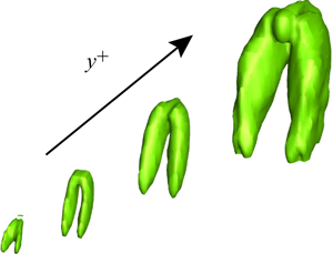
During the late stages of transition to turbulence, varicose instabilities are known to give rise to the formation of characteristic hairpin or lambda vortices which can be visualized by evaluating quantities such as the second invariant of the velocity gradient matrix, or the local minimum of the pressure. A visualization of the $Q$ field computed for the first symmetric CST-POD mode is presented in the last row of figure 7, and consistently shows a hairpin structure at all considered wall distances. In line with the velocity fluctuation fields, the size of the vortex increases with wall distance. More generally, the outcome demonstrates that although individual turbulent flow structures may become difficult to identify in developed turbulence, as previously noted by Schlatter et al. (Reference Schlatter, Li, Örlu, Hussain and Henningson2014), statistically these features persist in the leading CST-POD modes which represent the largest part of the fluctuation kinetic energy of the sampled extreme events.

Beyond the velocity and vortex fields, the varicose instability also generates a characteristic pattern in the production and dissipation of turbulent kinetic energy that was previously documented in the transitional setting. Specifically, a localized patch of extreme levels of dissipation of turbulent kinetic energy, and thus of velocity gradients, has been shown to emerge above a larger region of increased production of turbulent kinetic energy. Isosurfaces of the production and dissipation of turbulent kinetic energy, $P$ and $\varepsilon$, for the present case are presented in figure 8 and show qualitatively similar trends. Quantitative results in the form of a line plot through the streamwise and spanwise centre point, $\tilde {x}=0$, $\tilde {z}=0$, are presented in figure 9 for the cases $y^+=30$ and $y^+=70$. A sharp extremum in the dissipation is located above a wider maximum in the production of turbulent kinetic energy. These characteristic profiles can be interpreted as a signature of the varicose mode, and match those documented for transitional flow. Figure 12(b) of Hack & Moin (Reference Hack and Moin2018) presents the dissipation and production of turbulent kinetic energy along a line through the centre of a transitional hairpin vortex, which show the same qualitative profiles as the present results obtained for extreme events in developed turbulence.

Figure 8. Isosurfaces of dissipation (purple) and production (red) of turbulent kinetic energy at $\tilde {t}^+=0$ for the first symmetric CST-POD mode computed for extreme events at $y^+=70$.

Figure 9. Dissipation (dashed) and production (solid) of the first symmetric CST-POD mode at $\tilde {x}^+=0$, $\tilde {z}^+=0$, $\tilde {t}^+=0$, normalized by the maximum local dissipation value. (a) Extreme events at $y^+=30$. (b) Extreme events at $y^+=70$.

In the transitional setting, the still orderly flow field enables the unambiguous determination of the exponential property of the varicose mechanism, both through an analysis of the DNS flow field, and a linear stability analysis. The setting also allows insight into the full structure of the varicose instability, which gives rise to the particular patterns in the velocity and $Q$, $P$ and $\varepsilon$ fields. Considered as a whole, the agreement of this range of properties with those observed for the first symmetric CST-POD mode provide comprehensive evidence for the correspondence with the mechanisms inducing the eventual breakdown to turbulence in transitional flows. More specifically, the results strongly suggest that secondary exponential instability plays a key role in the generation of peak events in developed turbulence.

The visualizations presented in figure 7 suggest that the spatial extent of the flow structures grows with wall distance. Such behaviour would be consistent with the attached-eddy hypothesis by Townsend (Reference Townsend1961), which predicts a hierarchy of flow structures that scale with wall distance (see also Marusic & Monty (Reference Marusic and Monty2019), for a recent review). We quantify the scaling of the varicose mode by charting the normalized streamwise velocity fluctuation, $u'/\max (u')$, at the time of maximum dissipation, $\tilde {t}=0$, on lines parallel to $\tilde {z}^+$ at the streamwise centre of the sampling domain, $\tilde {x}=0$, see figure 10. The relevance of the results was augmented by additionally considering the first symmetric CST-POD modes computed for extreme dissipation events at the wall distances $y^+=50$ and $y^+=100$. At the smallest considered distance to the wall, $y^+=10$, the general shape of the profiles deviates from those at the other locations so that it was not meaningful to include this case. The results for the remaining five wall distances, $y^+=\{30,50,70,100,150\}$ show an effectively self-similar spanwise profile of the normalized streamwise velocity fluctuations. A local minimum at the centre is surrounded by local maxima to the left and right. The distance between the local maxima defines the characteristic length $\varLambda _S^+$ which is presented in figure 11(a) as a function of the wall distance. The scaling of $\varLambda _S^+$ with $y^+$ is approximated by the linear relation

(4.1)\begin{equation} \varLambda_S^+=\varLambda_{S0}^++B_Sy^+, \end{equation}

where $\varLambda _{S0}^+= 46$ and $B_S=1.16$, shown as a solid line in figure 11(a).

Figure 10. Normalized streamwise fluctuations, $u'/\text{max}(u')$, of the first symmetric CST-POD modes as a function of the transverse sampling coordinate, $\tilde {z}^+$, at $\tilde {t}=0$, $\tilde {x}=0$ for extreme events at $y^+=\{30,50,70,100,150\}$.

Figure 11. (a) Characteristic length, $\varLambda _S^+$ (symbols), and linear relation, $\varLambda _{S0}^++B_Sy^+$ (line). (b) Amplitude of the peak streamwise velocity fluctuations, $\text{max}(u'^+)$. First symmetric CST-POD modes at $\tilde {t}=0$, $\tilde {x}=0$ for extreme events at $y^+=\{30,50,70,100,150\}$.

The maximum streamwise fluctuations $u'^+$ of the first CST-POD modes are presented in figure 11(b). A moderate decay is observed with increasing distance to the wall. The present results thus closely link the self-similar occurrence of the varicose mode in developed turbulence to Townsend's attached-eddy hypothesis. We note that a similar result was obtained by Hack & Moin (Reference Hack and Moin2018), where the distance of the ‘legs’ of hairpin vortices in turbulence at moderate Reynolds number was shown to also follow a linear trend (see their figure 34b).

The results for the varicose mode have so far focused on the time instance at which the flow attains local dissipation maxima, $\tilde {t}=0$. The CST-POD analysis also incorporates the flow fields before and after this peak event, and thus provides insight into the dynamics that leads to their formation. Figure 12 presents side views through the spanwise centre of the sampling domain, $\tilde {z}=0$, showing isocontours of the streamwise velocity fluctuations for the considered five time instances. We note that owing to the scaling of the instability with wall distance, which also applies in the time dimension, the five time instances cover varying intervals relative to the characteristic time during which the events evolves in each case. The general trends at the different wall distances are nonetheless consistent. At the first considered time instance, a region of moderately faster fluid is layered above a region of relatively slower fluid in a configuration that augments the mean shear. A localized ejection at the streamwise centre of the plane gradually lifts up slower fluid from near the wall, which further enhances the local gradient in the normal dimension. At the time of the peak event, shown in the third row of the figure, a sharp normal gradient has formed in all cases near the wall distance at which the peak dissipation event is recorded. Past the peak event, the velocity patterns generally decay more rapidly than they have formed, consistent with the notion of a breakup event.

Figure 12. Side views showing contours of the streamwise velocity fluctuations, $u'$, of the first symmetric CST-POD modes. Twelve contour lines span the range from the minimum to the maximum of each mode. Dashed lines indicate negative values. Columns from left to right, extreme events at $y^+=10$, $30$, $70$ and $150$. Rows from top to bottom, $\tilde {t}=-2{\rm \Delta} t$, $\tilde {t}=-{\rm \Delta} t$, $\tilde {t}=0$, $\tilde {t}={\rm \Delta} t$ and $\tilde {t}=2{\rm \Delta} t$.

In summary, the presented results based on the first symmetric CST-POD mode demonstrate the occurrence of an effectively self-similar instability mechanism in the buffer and logarithmic layers of the turbulent channel. The identified structures agree with the varicose instability documented during the late stages of laminar–turbulent transition in a number of attributes, and thus provide compelling evidence for the equivalence of the underlying mechanism. In the following, we will explore whether the first anti-symmetric CST-POD mode may analogously be attributed to the sinuous type of instability mechanism.

5. The sinuous mode

In the literature on the instability of laminar streaks, the varicose mode discussed above is oftentimes overshadowed by the sinuous type of instability. The sinuous mode is commonly associated with inflection points in the transverse shear (Swearingen & Blackwelder Reference Swearingen and Blackwelder1987), and was found to be more unstable than the varicose type in both idealized (Andersson et al. Reference Andersson, Brandt, Bottaro and Henningson2001) and realistic (Hack & Zaki Reference Hack and Zaki2014) settings of streaks in pre-transitional zero-pressure-gradient boundary layers. Similar considerations of linear theory motivated (Waleffe Reference Waleffe1997) to base the model of the self-sustaining process of wall turbulence exclusively on the sinuous mode. It is nonetheless also known that minor changes to the flow setting, such as the presence of a moderate streamwise pressure gradient, can tilt the balance in favour of the varicose mode. The present results for developed turbulence show that the first symmetric CST-POD mode computed for samples conditioned on extreme dissipation events contains appreciably more energy, both in relative and absolute terms, than the first anti-symmetric mode. This outcome suggests that the sinuous instability may be potentially less relevant in developed turbulence than the varicose mode.

The sinuous type of secondary instability is commonly associated with the transverse shear generated between a pair of low-speed and high-speed streaks. While the sinuous instability does not generate distinct vortical structures such as the hairpins formed by the varicose instability, it induces a characteristic meandering of turbulent streaks, as reported by Hutchins & Marusic (Reference Hutchins and Marusic2007) and Lozano-Durán & Jiménez (Reference Lozano-Durán and Jiménez2014b). Like the varicose mode, the sinuous instability was unambiguously documented in the still orderly pre-transitional regime. It was shown that the undulation of the streak is accompanied by an anti-symmetric pattern of positive and negative patches in the normal fluctuation component, and a symmetric, but streamwise alternating pattern of fluctuations in the transverse fluctuation component.

Isosurfaces of the velocity components of the first anti-symmetric CST-POD mode are presented in figure 13. The streamwise component shows two very-large-scale high-speed and low-speed streaks in the left and right halves of the sampling domain. Depending on the wall distance, the streaks attain spanwise scales of up to hundreds of wall units and reach beyond the border of the sampling domain. They can be understood as primary perturbations in the flow which increase the spanwise shear, and thus give rise to a secondary instability. Since the CST-POD analysis does not distinguish between primary and secondary flow features, it is not possible to separate the sampled perturbation into primary and secondary contributions. At the same time, it is worth noting that a hypothetical subtraction of the primary streaks from the kinetic energy would tilt the energetic balance further in favour of the varicose instability modes whose symmetric CST-POD mode lacks this type of very-large-scale primary structure.

Figure 13. First anti-symmetric CST-POD mode at $\tilde {t} = 0$. Isosurfaces of positive values (white and purple) and negative values (black and red) at approximately 80 % of the maximum amplitude. Streamwise fluctuations, $u'$ (a), normal fluctuations, $v'$ (b), transverse fluctuations, $w'$ (c) and streamwise vorticity, $\omega'_x$ (d). Wall distances from left to right: $y^+ = 10$, $30$, $70$, $150$. A smoothing filter was applied to the streamwise vorticity field at $y^+=\{30,70,150\}$ for visualization purposes only.

An anti-symmetric arrangement of regions of negative and positive normal fluctuations is located at the streamwise centre of the sampling domain. The single patch of positive $w'$ at the centre effectively induces a local displacement of the streaks in the positive $z$ direction. In the absence of a distinguishing vortical structure that clearly identifies the sinuous mode, the last row of figure 13 presents the field of the streamwise vorticity,

(5.1)\begin{equation} \omega'_x=\frac{\partial w'}{\partial y}-\frac{\partial v'}{\partial z}. \end{equation}

In the transitional case, the sinuous streak instability was shown to generate a characteristic streamwise arrangement of segments of alternating sign of $\omega'_x$ (see e.g. figure 13 in Hack & Zaki Reference Hack and Zaki2014). A similar configuration is found in the current case, which supports the connection between the symmetric CST-POD mode and the sinuous type of streak instability.

Insight into the scaling of the sinuous instability mode is gained by evaluating the normalized spanwise fluctuation $w'/\max (w')$ at the time of highest dissipation, $\tilde {t}=0$, along a line at $\tilde {x}=0$, as presented in figure 14. Consistent with the symmetric case, the considered wall distances are $y^+=\{30,50,70,100,150\}$. The spanwise fluctuations describe approximately self-similar profiles. The characteristic length scale $\varLambda _A^+$, defined as the distance between the two local maxima in the spanwise velocity fluctuations, is presented in figure 15(a) as a function of the wall distance. The length scale follows the linear relation

(5.2)\begin{equation} \varLambda_A^+=\varLambda_{A0}^++B_Ay^+ \end{equation}

with $\varLambda _{A0}^+=12$ and $B_A=0.85$, represented by a solid line in figure 15(a). The amplitudes of the peak spanwise velocity fluctuations, $w'^+$, at the five considered wall distances are presented in figure 15(b) and show an approximately constant trend. Similar to the varicose mode, the sinuous instability thus describes an effectively self-similar mechanism consistent with the attached-eddy hypothesis.

Figure 14. Normalized transverse fluctuations, $w'/\text{max}(w')$, of the first anti-symmetric CST-POD modes as a function of the transverse sampling coordinate, $\tilde {z}^+$, at $\tilde {t}=0$, $\tilde {x}=0$ for extreme events at $y^+=\{30,50,70,100,150\}$.

Figure 15. (a) Characteristic length, $\varLambda _A^+$ (symbols), and linear relation, $\varLambda _{A0}^++B_A\,y^+$ (line). (b) Amplitude of the peak transverse velocity fluctuations, $\max (w'^+)$. First anti-symmetric CST-POD modes at $\tilde {t}=0$, $\tilde {x}=0$ for extreme events at $y^+=\{30,50,70,100,150\}$.

Lastly, the temporal evolution of the streamwise fluctuation field in cross-sections through the streamwise centre point, $\tilde {x}=0$, is visualized in figure 16 at five time instances. Similar to the varicose case, the scaling of the instability with wall distance implies that modes at small $y^+$ undergo a faster evolution relative to the time frame captured by the analysis. The pair of high-speed and low-speed streaks is present at all considered instances. At the second time instance, $\tilde {t}=-{\rm \Delta} t$, localized fluctuations of opposite sign of the large-scale streaks are observed near the bottom of the sampling domain for the cases $y^+=30$ and $y^+=70$. At the time of the dissipation event, $\tilde {t}=0$, the phase of the instability has changed so that the streamwise velocity perturbation matches that of the streaks. During the last two time instances, the localized instability decays, and the amplitudes of the streaks decrease so that at $\tilde {t}=2{\rm \Delta} t$, they are appreciably lower than at $\tilde {t}=-2{\rm \Delta} t$ for most of the considered wall distances. This outcome is consistent with the concept of a breakdown of the streaks that is induced by the instability. The case $y^+=10$ marks an exception to this behaviour in the sense that the streaks, maintain a comparably high amplitude past the peak event.

Figure 16. Cross-sections showing contours of the streamwise velocity fluctuations, $u'$, of the first anti-symmetric CST-POD modes. Twelve contour lines span the range from the minimum to the maximum of each mode. Dashed lines indicate negative values. Columns from left to right, extreme events at $y^+=10$, $30$, $70$ and $150$. Rows from top to bottom, $\tilde {t}=-2{\rm \Delta} t$, $\tilde {t}=-{\rm \Delta} t$, $\tilde {t}=0$, $\tilde {t}={\rm \Delta} t$ and $\tilde {t}=2{\rm \Delta} t$.