3.1. Near-wall behaviour of the source terms and Dehoux's model limitations

In the vicinity of a wall located at $y=0$, using the no-slip boundary condition and the divergence-free constraint, it is easy to show that the Taylor series expansions of the fluctuating velocities and temperature with respect to the wall-distance $y$ are written as

(3.1)\begin{equation} \left. \begin{array}{c@{}} u'(x,y,z,t)=a_{1}(x,z,t) y+a_{2}(x,z,t) y^{2}+ O(y^3), \\ v'(x,y,z,t)=b_{2}(x,z,t) y^{2}+b_{3}(x,z,t) y^{3}+ O(y^4), \\ w'(x,y,z,t)=c_{1}(x,z,t) y+c_{2}(x,z,t) y^{2}+ O(y^3),\\ \theta'(x,y,z,t)=t_{0}(x,z,t)+t_{1}(x,z,t) y+t_{2}(x,z,t)\, y^{2}+O(y^3). \end{array}\right\}\end{equation}

The coefficients $a_k, b_k, c_k$ and $t_k$ are random variables independent of $y$. In order to simplify the writing of the expressions, the dependency on $(x,z,t)$ is set aside. The asymptotic behaviour of $\overline {u^{'}_i\theta ^{'}}, k, \varepsilon , \overline {\theta ^{'2}}$ and $\varepsilon _\theta$ are easily deduced, as follows:

(3.2)\begin{gather} \left.\begin{array}{c@{}} \overline{u^{'}\theta{'}} = \overline{a_1 t_0} y + (\overline{a_1 t_1} + \overline{a_2 t_0}) y^2 + O(y^3), \\ \overline{v^{'}\theta{'}} = \overline{b_2 t_0} y^2 + (\overline{b_2 t_1} + \overline{b_3 t_0}) y^3 + O(y^4), \\ \overline{w^{'}\theta{'}} = \overline{c_1 t_0} y + (\overline{c_1 t_1} + \overline{c_2 t_0}) y^2 + O(y^3), \end{array}\right\} \end{gather}

(3.3)\begin{gather}k = \tfrac{1}{2} \overline{u^{'}_iu^{'}_i} = \tfrac{1}{2} ( \overline{a_1^2} + \overline{c_1^2} ) y^2 + O(y^3), \end{gather}

(3.4)\begin{gather}\varepsilon = \nu \overline{\frac{\partial u_i^{'}}{\partial x_k} \frac{\partial u_i^{'}}{\partial x_k}} = \nu ( \overline{a_1^2} + \overline{c_1^2} ) + O(y), \end{gather}

(3.5)\begin{gather}\overline{\theta'^2} = \overline{t_0^2} + 2\overline{t_0 t_1} y + (\overline{t_1^2} + 2\overline{t_0 t_2} )y^2 + O(y^3), \end{gather}

(3.6)\begin{align} \varepsilon_{\theta}&= \kappa \overline{\frac{\partial\theta'}{\partial x_k}\frac{\partial\theta'}{\partial x_k}} = \kappa \left[ \overline{\left(\frac{\partial t_{0}}{\partial x} \right)^{2}} + \overline{t_{1}^{2}} + \overline{\left(\frac{\partial t_{0}}{\partial z} \right)^{2}} \right] + \kappa \left[ 2\overline{\frac{\partial t_{0}}{\partial x }\frac{\partial t_{1}}{\partial x }} + 4 \overline{t_{1} t_{2}} + 2 \overline{\frac{\partial t_{0}}{\partial z }\frac{\partial t_{1}}{\partial z }} \right] y \nonumber\\ &\quad + \kappa \left[ \overline{\left(\frac{\partial t_{1}}{\partial x} \right)^{2}} + 2 \overline{\frac{\partial t_{0}}{\partial x }\frac{\partial t_{2}}{\partial x }} + 4 \overline{t_{2}^{2}} + 6 \overline{t_{1} t_{3}} + \overline{\left( \frac{\partial t_{1}}{\partial z} \right)^{2}} + 2 \overline{\frac{\partial t_{0}}{\partial z }\frac{\partial t_{2}}{\partial z }} \right] y^{2} + O(y^3). \end{align}

The leading-order terms of the Taylor series expansions of the thermal variables depend on the temperature boundary condition. For an imposed temperature, $\theta '$ goes to zero at the wall, and therefore $t_0=0$. For an imposed heat flux, $t_0 \neq 0$, but the derivative of $\theta '$ in the wall-normal direction is zero, so that $t_1=0$. Finally, for CHT, there is no specific simplification: $t_0$ and $t_1$ can take any value.

The asymptotic behaviour of the exact source terms of the turbulent heat flux transport equations can then be determined using the Taylor series expansions presented above. It is not necessary to detail the calculations here, and only the final results are presented in table 1 for the streamwise and spanwise components and in table 2 for the wall-normal component. Three important observations can be made on the basis of these tables. (i) The behaviour of the terms of the transport equations for $\overline {u' \theta '}$ and $\overline {w' \theta '}$ is the same, as well as their expansions in (3.2), so that it is not necessary to detail the behaviour of both components: in the rest of this paper, only the component $\overline {u' \theta '}$ is considered. (ii) The asymptotic behaviour of these exact source terms depends on the thermal boundary condition to such an extent that the terms appearing at leading order are different. For instance, for the wall-normal component (table 2), the dissipation term $\varepsilon _{\theta i}$ is a dominant term for an imposed temperature, whereas it is negligible in the other two cases. (iii) The production terms $P_{\theta i}^{U}$ and $P_{\theta i}^{T}$ and the turbulent diffusion term $D_{\theta i}^{t}$ are always negligible compared to the molecular diffusion $D_{\theta i}^{\nu + \kappa }$, the scrambling $\phi _{\theta i}$ and the dissipation $\varepsilon _{\theta i}$ terms; consequently it is sufficient to consider the last three terms in the asymptotic analysis of the transport equation for the turbulent heat flux. Therefore, the analysis focuses on the near-wall balance

(3.7)\begin{equation} D_{\theta i}^{\nu + \kappa} + \phi_{\theta i} - \varepsilon_{\theta i} =0,\end{equation}

that must be satisfied for all the cases.

Table 1. Asymptotic behaviour of the source terms appearing in the exact transport equations for $\overline {u^{'}\theta ^{'}}$ and $\overline {w^{'}\theta ^{'}}$.

Table 2. Asymptotic behaviour of the source terms appearing in the exact transport equation for $\overline {v^{'}\theta ^{'}}$.

Dehoux's model was derived in order to satisfy (3.7) in the case of an imposed temperature at the wall. One of the limitations of this model is that it makes use of the algebraic expression (2.15) to represent the thermal-to-mechanical time scale ratio $R$, in order to avoid the resolution of a transport equation for the dissipation rate of the variance, $\varepsilon _\theta$. As shown is table 3, the wall-limiting behaviour of $R$ strongly depends on the thermal boundary condition: the exact $R$ goes to the Prandtl number at the wall for an imposed temperature, while it tends to infinity in the other two cases. However, in all cases, the algebraic model (2.15) tends to the Prandtl number.

Table 3. Asymptotic behaviour of the exact expression of the thermal-to-mechanical time scale ratio $R$.

This situation is illustrated by figure 1, which shows an a priori evaluation of this algebraic model for $R$; the elliptic equation (2.8) is solved by using the length scale computed from the DNS data, in order to evaluate the value of $R$ given by the algebraic relation (2.15), which is independent of the thermal boundary condition. The comparison made in figure 1 with the exact value of $R$ given by (2.14) extracted from the DNS databases shows that this model for $R$ is not sufficiently general, since the near-wall behaviour of the model is not sensitive to the thermal boundary condition.

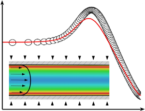
Figure 1. Thermal-to-mechanical time scale ratio $R$ for different temperature boundary conditions. Channel flow DNS data of Flageul et al. (Reference Flageul, Benhamadouche, Lamballais and Laurence2015). For the CHT case, the solid and the fluid have the same thermal conductivity and diffusivity.

The main consequence of this lack of generality of the model for $R$ is that the models (2.10) and (2.11) for the scrambling term $\phi _{\theta i}$ and the dissipation term $\varepsilon _{\theta i}$, respectively, are not compatible with an imposed heat flux or CHT. This can be observed in figures 2 and 3 for $\varepsilon _{\theta i}$, and in figure 4 for $\phi _{\theta i}$. The scrambling term is only shown for CHT as the profiles are very similar with an imposed heat flux. For the tangential component $\varepsilon _{\theta 1}$ of the dissipation term, the problem comes from the near-wall contribution $\varepsilon _{\theta 1}^w$ given by (2.11), which goes to infinity at the wall as $1/y$, while the asymptotic analysis of the exact term shows that it goes to zero as $y$ for an imposed flux and to a constant for CHT (table 1). In contrast, for $\phi _{\theta 1}$, the near-wall contribution $\phi _{\theta 1}^w$ is correct, but its behaviour is strongly perturbed by the component $\phi _{\theta 1}^h$ given by (2.9) that goes to infinity at the wall and is not sufficiently damped by the factor $\alpha _\theta$ in (2.7). Moreover, although the situation seems less critical for the normal component of the dissipation term, its behaviour is also not correct as it tends towards a non-zero value at the wall. Therefore, in order to derive a model valid for an imposed heat flux and CHT as well as for an imposed wall temperature, the asymptotic analysis of Dehoux et al. (Reference Dehoux, Benhamadouche and Manceau2017) must be extended to various thermal boundary conditions, which is done in § 3.2.

Figure 2. A priori evaluation of the dissipation term for an imposed heat flux. (a) Streamwise component; (b) wall-normal component. Channel flow DNS data of Flageul et al. (Reference Flageul, Benhamadouche, Lamballais and Laurence2015).

Figure 3. A priori evaluation of the dissipation term for CHT. (a) Streamwise component; (b) wall-normal component. Channel flow DNS data of Flageul et al. (Reference Flageul, Benhamadouche, Lamballais and Laurence2015).

Figure 4. A priori evaluation of the scrambling term for CHT. (a) Streamwise component; (b) wall-normal component. Channel flow DNS data of Flageul et al. (Reference Flageul, Benhamadouche, Lamballais and Laurence2015).

3.2. Asymptotic behaviour of $\overline {u_i' \theta '}$ with the right asymptotic behaviour of $R$

In the previous section, it has been concluded that the validity of Dehoux's model is limited to the case of an imposed temperature, mainly due to the model (2.15) for $R$, which is not sufficiently general. However, the following question must also be raised: Would correcting the expression for $R$ be sufficient for the model to give the correct asymptotic behaviour of turbulent heat flux? We will see in the present section that the answer is no.

The procedure is as follows: it is assumed that the exact asymptotic behaviour of the thermal-to-mechanical time scale ratio $R$ is respected in all the cases; the near-wall behaviour of the solution of the modelled transport equation for the turbulent heat flux is analysed and compared with the exact behaviour, in order to identify how the model can be made more general.

If one uses the exact asymptotic behaviour of $R$, Dehoux's model yields $\varepsilon _{\theta 1}^w = O(1)$ and $\varepsilon _{\theta 2}^w = O(y)$ whatever the temperature boundary condition at the wall. By comparing with tables 1 and 2, it can be seen that the model is correct for both an imposed temperature condition and CHT. However, for an imposed heat flux, the near-wall behaviour of $\varepsilon _{\theta i}^w$ is one order below that of the exact term. After considering several options, we have not found any solution to modify the behaviour in this case without spoiling the behaviour in the other two cases. Therefore, our strategy consists in keeping the near-wall model $\varepsilon _{\theta i}^w$ proposed by Dehoux et al. (Reference Dehoux, Benhamadouche and Manceau2017), and to account for the discrepancy with the exact behaviour in the case of imposed heat flux in the derivation of the model $\phi _{\theta i}^w$. Indeed, as mentioned above, as long as the near-wall balance between the molecular diffusion $D_{\theta i}^{\nu + \kappa }$, the scrambling term $\phi _{\theta i}$ and the dissipation term $\varepsilon _{\theta i}$ is satisfied, the solution of the transport equation for the turbulent heat flux will have the correct asymptotic behaviour.

Dehoux's model for $\varepsilon _{\theta i}^w$ is associated with the model of Shikazono & Kasagi (Reference Shikazono and Kasagi1996) for $D_{\theta i}^{\nu +\kappa }$ (2.6). The model $\phi _{\theta i}^w$ must be derived in such a way that the correct near-wall balance (3.7) is ensured. As demonstrated below, this can be achieved simply by modifying the coefficient $\beta$ in (2.10).

In order to determine the relevant value of $\beta$, it is necessary to analyse the asymptotic behaviour of the solution of the transport equation for the turbulent heat flux, following the same methodology as proposed by Durbin (Reference Durbin1991) for the Reynolds-stress tensor. Considering only the dominant terms in the near-wall region (3.7), solutions are sought under the form of a Taylor series

(3.8)\begin{equation} \overline{u^{'} \theta^{'}} = A_1 y + B_1 y^2 + C_1 y^3 + O(y^4) \end{equation}

and

(3.9)\begin{equation} \overline{v^{'} \theta^{'}} = A_2 y + B_2 y^2 + C_2 y^3 + O(y^4). \end{equation}

Introducing these Taylor series into (3.7) leads to constraints that the expansion coefficients $A_i, B_i$ and $C_i$ must satisfy, and, consequently, the asymptotic behaviour of the solutions can be determined. The model $\phi _{\theta i}^w$ must be formulated in order for these solutions to match the exact asymptotic behaviour of the turbulent heat flux.

Using the models (2.6), (2.10) and (2.11) for $D_{\theta i}^{\nu +\kappa }, \varepsilon _{\theta i}^w$ and $\phi _{\theta i}^w$, respectively, the near-wall balance (3.7) writes as

(3.10)\begin{equation} \frac{\nu + \kappa}{2} \frac{\partial^{2} \overline{u^{'} \theta^{'}}}{\partial y^{2}} + \frac{\nu + \kappa}{2} \left(\frac{\partial^{2} \overline{u^{'} \theta^{'}}}{\partial x^{2}} + \frac{\partial^{2} \overline{u^{'} \theta^{'}}}{\partial z^{2}} \right) = ( \nu + \kappa ) \psi \sqrt{\frac{1}{2 \nu \mathcal{T}}} \overline{u^{'} \theta^{'}}\end{equation}

and

(3.11)\begin{align} &\left(\frac{2}{3} \nu + \frac{1}{3} \kappa \right) \frac{\partial^{2} \overline{v^{'} \theta^{'}}}{\partial y^{2}} +\left(\frac{2}{3} \nu + \frac{1}{3} \kappa \right) \left(\frac{\partial^{2} \overline{v^{'} \theta^{'}}}{\partial x^{2}} + \frac{\partial^{2} \overline{v^{'} \theta^{'}}}{\partial z^{2}} \right)\nonumber\\ &\quad = 2( \nu + \kappa ) \psi \sqrt{\frac{1}{2 \nu \mathcal{T}}} \overline{v^{'} \theta^{'}} + \beta \frac{1}{\mathcal{T}} \overline{v^{'} \theta^{'}}, \end{align}

where

(3.12)\begin{equation} \psi = \sqrt{\frac{\varepsilon_\theta}{\kappa \overline{\theta^{'2}}}}. \end{equation}

These equations can be simplified based on the expression (2.13) for $C_\varepsilon$; the Taylor series expansion $1/\mathcal {T} = 2 \nu /y^2 (1 + a_\mathcal {T} y + b_\mathcal {T} y^2 + O(y^3) )$ deduced from the Taylor series expansions of the turbulent kinetic energy $k$ and its dissipation rate $\varepsilon$ ((3.3) and (3.4)); the fact that the term $(1-\alpha _\theta ) ({P_k}/{\varepsilon })$ that appears in the models $\varepsilon _{\theta i}^w$ and $\phi _{\theta i}^w$ behaves as $y^3$ in the vicinity of the wall; and the general forms of the solutions (3.8) and (3.9). Equations (3.10) and (3.11) then become

(3.13)\begin{align} & (\nu + \kappa) B_1+( 3 (\nu + \kappa ) C_1 + \chi_{A_1} ) y + O(y^2) \nonumber\\ &\quad = (\nu + \kappa ) \psi [A_1 + ( B_1 + \tfrac{1}{2}a_\mathcal{T} A_1) y + ( \tfrac{1}{2} b_\mathcal{T} A_1 + \tfrac{1}{2} a_\mathcal{T} B_1 + C_1) y^2+ O(y^2) ] \end{align}

and

(3.14)\begin{align} & \left(\frac{4}{3} \nu + \frac{2}{3} \kappa \right) B_2 + ( (4 \nu + 2 \kappa ) C_2 + \chi_{A_2}) y + O(y^2) \nonumber\\ &\quad = (\nu + \kappa ) \psi \left[A_2 + \left( B_2 + \tfrac{1}{2}a_\mathcal{T} A_2\right) y + \left( \tfrac{1}{2} b_\mathcal{T} A_2 + \tfrac{1}{2} a_\mathcal{T} B_2 + C_2\right) y^2+ O(y^2) \right] \nonumber\\ &\,\,\qquad 2 \nu \beta \left[ \frac{A_2}{y} + ( B_2 +a_\mathcal{T} A_2 ) + (b_\mathcal{T} A_2 +a_\mathcal{T} B_2 +C_2) y + O(y)\right], \end{align}

where

(3.15a,b)\begin{equation} \chi_{A_1} = \frac{\nu + \kappa}{2} \left(\frac{\partial^{2} A_1}{\partial x^{2}} + \frac{\partial^{2}A_1}{\partial z^{2}} \right)\quad \text{and} \quad \chi_{A_2} = \left(\frac{2}{3} \nu + \frac{1}{3} \kappa \right) \left(\frac{\partial^{2} A_2}{\partial x^{2}} + \frac{\partial^{2}A_2}{\partial z^{2}} \right). \end{equation}

In order to obtain this development up to order 1 and noticing that the lowest order of $\overline {u^{'} \theta ^{'}}$ and $\overline {v^{'} \theta ^{'}}$ is 1, the Taylor series expansion of $1/\mathcal {T}$ had to be carried out up to order 2 as $\psi$ might introduce a term which behaves as $1/y$ at the wall.

As the Taylor series expansion of $\psi$ depends on the thermal boundary condition, two cases need to be considered separately to obtain relations or constraints on the coefficients $A_i, B_i$ and $C_i$; on the one hand, an imposed temperature at the wall and on the other hand, an imposed heat flux or CHT.

3.2.1. Imposed wall temperature

The case of an imposed wall temperature is considered first, for which $t_0=0$. Using the Taylor series expansions of $\overline {\theta ^{'2}}$ and $\varepsilon _\theta$ given by (3.5) and (3.6), respectively, it is found that $\psi = 1/y ( 1 + a_\psi y + b_\psi y^2 + O (y^{3}) )$, such that for the streamwise component, (3.13) writes as

(3.16)\begin{equation} (\nu + \kappa) B_1+ O(y) = (\nu + \kappa ) \frac{A_1}{y} + (\nu + \kappa ) \left[ \left(\frac{1}{2} a_\mathcal{T} + a_\psi \right) A_1 + B_1 \right] +O(y).\end{equation}

For function (3.8) to be a solution of (3.16), the two sides of (3.16) must balance at each order $y^n$. Balancing the terms at the orders $n=-1$ and $n=0$ yields

(3.17)\begin{equation} \left. \begin{array}{c@{}} 0= (\nu + \kappa ) A_1, \\ (\nu + \kappa ) B_1 = (\nu + \kappa ) [ (\tfrac{1}{2} a_\mathcal{T} + a_\psi ) A_1 + B_1 ]. \end{array}\right\}\end{equation}

The first relation shows that $A_1=0$. With $A_1=0$, the second relation shows that there is no particular constraint on $B_1$ since any value satisfies this equation. In conclusion, any solution $\overline {u'\theta '}$ of (3.10) is of the form $\overline {u^{'} \theta ^{'}} = B_1 y^2 +O(y^3)$, which is the expected behaviour for an imposed temperature at the wall. As mentioned above, this conclusion holds for $\overline {w'\theta '}$ as well, i.e. $\overline {w^{'} \theta ^{'}} = B_3 y^2 +O(y^3)$.

For the wall-normal component $\overline {v'\theta '}$, considering that $\beta$ goes to $1$ at the wall as in Dehoux's algebraic model (see (2.15)), (3.14) leads, after similar algebraic manipulations, to consider the terms from order $n=-1$ up to order $n=1$ (note that the second-order term in the Taylor series expansion of $\psi$ must be taken into account for this component).

The orders $n=-1$ and $n=0$ yield $A_2=B_2=0$, respectively. The order $n=1$ gives, using the fact that $\beta$ tends to a constant value at the wall, $(4 \nu + 2 \kappa )(C_2 + \chi _{A_2}) = (4 \nu + 2 \kappa ) C_2$. Since $A_2=0, \chi _{A_2}$ is zero as well, and it is seen that any value of $C_2$ satisfies the relation. Therefore, any solution $\overline {v'\theta '}$ of the equation is of the form $\overline {v^{'} \theta ^{'}} = C_2 y^3 + O(y^4)$, as expected for this component.

3.2.2. Imposed wall heat flux and conjugate heat transfer

As mentioned above, the case of an imposed heat flux ($t_1$ is zero) and the case of CHT ($t_0$ and $t_1$ are both non-zero) can be treated simultaneously. Indeed, the asymptotic behaviour of $\psi$ obtained using (3.5) and (3.6) is in both cases equal to $\psi = O(1)$. The objective is again to obtain the expected asymptotic behaviour at the wall $\overline {u^{'} \theta ^{'}}=O(y)$ and $\overline {v^{'} \theta ^{'}}=O(y^2)$. As $\psi$ goes to a constant at the wall, it is enough here to use the Taylor series expansion of $\psi$ up to order 1: $\psi = \psi _0 + a'_\psi y + O(y^2)$.

After some algebraic manipulations, it is found that, for the streamwise component, it is sufficient to consider the order $n=0$, which leads to $(\nu + \kappa ) B_1 = (\nu + \kappa ) \psi _0 A_1$. Since $\psi _0 \neq 0$, this equation imposes a relation between $A_1$ and $B_1$, without constraining the value of $A_1$ to be zero. Therefore, $\overline {u^{'} \theta ^{'}}=O (y)$, which is the expected behaviour of the solutions. The analysis is valid for $\overline {w^{'} \theta ^{'}}$ as well, i.e. $\overline {w^{'} \theta ^{'}}=O (y)$. For the wall-normal component, at orders $n=-1$ and $n=0$, (3.11) yields

(3.18)\begin{equation} \left.\begin{array}{c}0= 2 \beta \nu A_2 ,\\ \frac{1}{3} (4 \nu + 2\kappa ) B_2 = 2 (\nu + \kappa ) \psi_0 A_2 + 2 \nu\beta (a_\mathcal{T} A_2 + B_2 ), \end{array}\right\} \end{equation}

respectively. The first relation gives $A_2=0$ as far as $\beta \neq 0$. We have reached the point where we must make the correct choice for $\beta$ in order to impose $\overline {v^{'} \theta ^{'}}=O (y^2)$: $\beta$ must be chosen in such a way that the second line of (3.18) is satisfied for any non-zero value of $B_2$. The equation that must be satisfied is

(3.19)\begin{equation} \beta= \frac{2}{3} +\frac{1}{3}\frac{1}{Pr},\end{equation}

or, more generally, $\beta$ must asymptote to this value at the wall in the case of an imposed heat flux or CHT.

This section illustrates the fact that Dehoux's model, with $\beta =\sqrt {Pr}/\sqrt {R}$, designed for an imposed wall temperature, is not valid for an imposed heat flux and CHT, even if a correct model for $R$ is used, as $\beta$ tends to $0$ with this formulation. In order to extend the validity of the model, the $\beta$ coefficient, which enters the near-wall model $\phi _{\theta i}^w$, must tend to $1$ at the wall for an imposed temperature and to $2/3 + 1/(3Pr)$ for the other two cases. The next section is devoted to the derivation of such a model.

3.3. A new model for the scrambling term and a priori tests

In the present section, Dehoux's model is extended to various thermal boundary conditions, following the findings of the asymptotic analysis performed in the previous section. The model is first derived, then an a priori evaluation of the model using the DNS databases of Flageul et al. (Reference Flageul, Benhamadouche, Lamballais and Laurence2015) is performed.

As concluded in the previous section, the model must be able to naturally distinguish the type of the thermal boundary condition at the wall in order to adapt the limiting behaviour of the $\beta$ coefficient. Now, to write a general model, i.e. a model that is expressed in the same form in all configurations, it is necessary to involve in its expression one or several quantities that are sensitive to boundary conditions. Only quantities that are solutions of a second-order differential equation exhibit this property. In the context of elliptic blending, it is tempting to rely on the $\alpha _\theta$ variable, whose wall boundary condition could be defined differently depending on the thermal boundary condition at the same wall. Unfortunately, $\alpha _\theta$ is involved in different terms of the model and such an approach would skew the asymptotic behaviour of these terms. We have come to the conclusion that the only way to sensitize the model to thermal boundary conditions is to involve a dimensionless parameter dependent on $\overline {\theta ^{'2}}, \varepsilon _\theta$ or both. Thus, the key parameter that enters the model is the thermal-to-mechanical time scale ratio $R={\mathcal {T}_\theta }/{\mathcal {T}}$. Indeed, figure 1 and table 3 show that $R$ tends to the Prandtl number at the wall for an imposed temperature and to infinity in other cases. Consequently, the ratio $\sqrt {{Pr}}/\sqrt {{R}}$ is used in the expression for $\beta$ to sensitize the model to the type of wall thermal boundary condition. The proposed expression is

(3.20)\begin{equation} \beta = \frac{2}{3} +\frac{1}{3}\frac{1}{Pr} + \frac{1}{3} \frac{\sqrt{Pr}}{\sqrt{R}}\left(1-\frac{1}{Pr}\right), \end{equation}

such that $\beta$ tends to $1$ for an imposed temperature ($R \to Pr$) and to $2/3+1/(3Pr)$ for the two other thermal boundary conditions ($R \to \infty$). In contrast, as mentioned above, $\gamma$ in (2.11) does not need to be modified, and the expression of Dehoux et al. (Reference Dehoux, Benhamadouche and Manceau2017),

(3.21)\begin{equation} \gamma = \frac{\sqrt{Pr}}{\sqrt{R}},\end{equation}

is used. With this simple but decisive modification of the model, the near-wall balance between the molecular diffusion $D_{\theta i}^{\nu + \kappa }$, the scrambling $\phi _{\theta i}$ and the dissipation $\varepsilon _{\theta i}$ terms, (3.7), is respected in the near-wall region, which is the necessary condition for reproducing the adequate asymptotic behaviour of the turbulent heat flux components, as demonstrated in § 3.2.

It is worth noting again that, for this model to be valid for the three types of wall boundary conditions, it is necessary for the thermal-to-mechanical time scale ratio $R$ to have the correct limiting behaviour at the wall, which will require solving a transport equation for the temperature variance $\overline {{\theta '}^2}$ and its dissipation $\varepsilon _\theta$, rather than using a simple algebraic relation such as (2.15). In particular, a model for $\varepsilon _\theta$, asymptotically correct for all types of thermal boundary conditions, is required. Therefore, a specific model has been developed, which is presented in § 4.

One could legitimately point out that solving additional transport equations for $\overline {{\theta '}^2}$ and $\varepsilon _\theta$ is particularly costly when it is simply a matter of sensitizing the model to thermal boundary conditions. On the one hand, as noted above, only a non-dimensional parameter constructed from these variables can define a sufficiently general model. On the other hand, it is important to remember that, as mentioned in the introduction, one of the main interests in developing a model valid in CHT is to be able to estimate thermal fatigue from the temperature variance in the solid. It is therefore necessary to solve the equation of $\overline {{\theta '}^2}$, but also of $\varepsilon _\theta$, since, as will be shown in § 4, the asymptotic behaviour of $\varepsilon _\theta$ is complex and has a strong influence on that of $\overline {{\theta '}^2}$.

A priori tests are carried out using recent DNS data of Flageul et al. (Reference Flageul, Benhamadouche, Lamballais and Laurence2015) of a channel flow in the forced convection regime, for different boundary conditions: imposed temperature, imposed heat flux and CHT. The flow is driven by a pressure gradient in the streamwise direction. The temperature is considered as a passive scalar and the flow is periodic in the streamwise and spanwise directions. The test case is defined by two non-dimensional numbers, the friction Reynolds number $Re_\tau =\delta u_\tau /\nu =149$ and the Prandtl number $Pr=0.71$. When the solid part is resolved in the DNS computations, the continuity of the heat flux is imposed at the fluid–solid interface. Note that the CHT case considered herein is the case considered by Flageul et al. (Reference Flageul, Benhamadouche, Lamballais and Laurence2015), where the solid and the fluid have the same thermal conductivity and diffusivity and thus the dissipation rate of the temperature variance is continuous at the fluid–solid interface. Reproducing this case is already a big challenge, and is sufficient to validate the new model for the turbulent heat flux since its asymptotic behaviour is not affected by these physical properties.

The case of an imposed temperature at the wall is considered first. Figure 5 compares with DNS data the sum of the molecular diffusion, the scrambling and the dissipation terms obtained with Dehoux's model and the new model. As mentioned above, these terms are dominant in the near-wall budget and determine the asymptotic behaviour of the turbulent heat flux components. It can be seen that the new model correctly reproduces the balance of the three terms in the case of an imposed temperature at the wall. The results given by the new model are slightly less accurate than those given by Dehoux's model in the buffer layer, but this is not a significant problem since, in this region, the budgets of the turbulent heat flux components are dominated by the production terms, contrary to the very near-wall balance (Flageul et al. Reference Flageul, Benhamadouche, Lamballais and Laurence2015). The two models are asymptotically identical for this type of boundary conditions, but the coefficient $\beta$ is modelled in a different way, since (3.20) is used for the new model.

Figure 5. Sum of the molecular diffusion, the scrambling and the dissipation terms for an imposed temperature. (a) Streamwise component; (b) wall-normal component.

The same comparisons are performed in figures 6 and 7 for the cases with an imposed heat flux and with CHT, respectively. Contrary to the previous case, a superior capacity of the new model to estimate the streamwise component of the balance can be observed. Indeed, with Dehoux's model, this component goes to infinity in both cases. This problem is mainly due to the near-wall model for $\varepsilon _{\theta 1}$ which goes to infinity at the wall as shown in figure 2(a) for an imposed heat flux and in figure 3(a) for CHT. In the new model, this term tends to a constant for both boundary conditions, which is the expected asymptotic behaviour. Moreover, figure 4(a) shows that $\phi _{\theta 1}$ is better estimated with the new model (the same profiles hold for an imposed heat flux), since it tends to zero at the wall as in the reference data. Note that although only the difference $\phi _{\theta i}-\varepsilon _{\theta i}$ appears in the transport equation for turbulent heat flux, it is important to correctly model the two terms individually, since the model for $\varepsilon _{\theta i}$ also appears in the model for $P_{\varepsilon _{\theta }}^1$ described in § 4.1.

Figure 6. Sum of the molecular diffusion, the scrambling and the dissipation terms for an imposed heat flux. (a) Streamwise component; (b) wall-normal component.

Figure 7. Sum of the molecular diffusion, the scrambling and the dissipation terms for CHT. (a) Streamwise component; (b) wall-normal component.

Figures 6(b) and 7(b) show a better estimate of the balance with the new model for the wall-normal component. Since figure 4(b) shows that the two models give virtually identical results in the near-wall region for $\phi _{\theta 2}$, the improvement is only due to the better prediction of $\varepsilon _{\theta 2}$ as it can be observed in figures 2(b) and 3(b), respectively. Indeed, $\varepsilon _{\theta 2}$ tends to zero at the wall with the new model as DNS data does, whereas, with Dehoux's model, it goes to a constant. It is observed that the new model does not improve the results in the buffer layer: this is an intrinsic limitation of the elliptic blending approach which extends the validity of high-Reynolds-number models, i.e. valid only far from the wall, to the near-wall region by satisfying the asymptotic behaviour observed in the viscous sublayer without imposing any constraint in the buffer layer.

To conclude, unlike Dehoux's model which is exclusively valid for an imposed temperature at the wall, the a priori tests confirm that the new model satisfies the asymptotic behaviour of the dominant terms of near-wall budget of the turbulent heat flux. However, for this model to be complete and valid, the thermal-to-mechanical time scale ratio $R$ must have the correct asymptotic behaviour whatever the temperature boundary condition. Modelling the dissipation rate of the temperature variance $\varepsilon _\theta$ is then needed. The computation of $\varepsilon _\theta$ will also make it possible to better predict the temperature variance, without the need for an algebraic formulation of $R$.

4.1. Production terms $P_{\varepsilon _\theta }^1$ and $P_{\varepsilon _\theta }^2$

The production term by the mean temperature gradient reads as

(4.2)\begin{equation} P_{\varepsilon_\theta}^1=- 2 \kappa \frac{\partial \bar{\theta}}{\partial x_j}\overline{\frac{\partial u_j'}{\partial x_k}\frac{\partial \theta'}{\partial x_k}}.\end{equation}

As this term is directly related to the dissipation tensor involved in the transport equation for the turbulent heat flux, $\varepsilon _{\theta j} = (\nu +\kappa ) \overline {({\partial u_j'}/{\partial x_k})({\partial \theta '}/{\partial x_k})}$, it is simply modelled as

(4.3)\begin{equation} P_{\varepsilon_\theta}^1 = - \frac{2}{1+Pr} \varepsilon_{\theta j} \frac{\partial \bar{\theta}}{\partial x_j}, \end{equation}

where $\varepsilon _{\theta j} = (1-\alpha _\theta ) \varepsilon _{\theta j}^w$ and $\varepsilon _{\theta j}^w$ is given by (2.11).

The production term by the mean velocity gradient reads as

(4.4)\begin{equation} P_{\varepsilon_\theta}^2=-2 \kappa \frac{\partial \overline{u_j}}{\partial x_k}\ \overline{\frac{\partial \theta'}{\partial x_k}\frac{\partial \theta'}{\partial x_j}}. \end{equation}

The tensor $\varepsilon _{ij}^{\theta } = 2 \kappa \overline {({\partial \theta '}/{\partial x_i})({\partial \theta '}/{\partial x_j})}$ is very similar to the dissipation tensor $\varepsilon _{ij}$ in the Reynolds-stress tensor equation, and, in particular, is linked to the smallest scales of the turbulent thermal field. Therefore, the same modelling strategy as for $\varepsilon _{ij}$ is adopted: it is assumed that $\varepsilon _{ij}^{\theta }$ is isotropic far from the wall and exhibits the same anisotropy as the Reynolds-stress tensor in the near-wall region, such that it is formulated as

(4.5)\begin{equation} \varepsilon_{ij}^{\theta} = (1-\alpha_\theta) \varepsilon_{ij}^{\theta w} + \alpha_\theta \varepsilon_{ij}^{\theta h}, \end{equation}

where

(4.6a,b)\begin{equation} \varepsilon_{ij}^{\theta h} = \tfrac{2}{3} \varepsilon_\theta \delta_{ij} \quad \text{and} \quad \varepsilon_{ij}^{\theta w} = \frac{\overline{u^{'}_i u^{'}_j}}{k} \varepsilon_\theta. \end{equation}

Hence, the production by the mean velocity gradient is modelled as

(4.7)\begin{equation} P_{\varepsilon_\theta}^2 = -c_{\varepsilon_{\theta 1}} \varepsilon_{jk}^{\theta} \frac{\partial \overline{u_j}}{\partial x_k}. \end{equation}

For the sake of concision, the a priori estimates of the two production terms are only shown for CHT in figure 9. Conclusions are similar for the two other boundary conditions. For $P_{\varepsilon _\theta }^1$, the near-wall behaviour of DNS is correctly recovered. A relatively weak prediction in the buffer layer is observed (for all the boundary conditions) which is due to an overestimated dissipation rate $\varepsilon _{\theta 2}$ in this region. For $P_{\varepsilon _\theta }^2$, the predictions are satisfactory far from the wall. The modelled production goes to zero at the wall whatever the thermal boundary conditions, which is not the case according to DNS data for CHT. However, in the latter case, the production by the mean velocity gradient tends towards a small non-zero value at the wall which makes the model acceptable (figure 10).

Figure 9. A priori tests: (a) $P_{\varepsilon _\theta }^1$ and (b) $P_{\varepsilon _\theta }^2$ for CHT.

Figure 10. (a) The dynamic time scale ratio $\mathcal {T}$ and (b) the thermal time scale ratio $\mathcal {T}_\theta$ from the DNS data of Flageul et al. (Reference Flageul, Benhamadouche, Lamballais and Laurence2015, Reference Flageul, Benhamadouche, Lamballais and Laurence2017) for different kinds of temperature boundary conditions.

4.2. Difference between the turbulent production and the dissipation $P_{\varepsilon _\theta }^4 - Y_{\varepsilon _\theta }$

The difference between the turbulent production, $P_{\varepsilon _\theta }^4$, and the dissipation rate of $\varepsilon _\theta , Y_{\varepsilon _\theta }$, reads as

(4.8)\begin{equation} P_{\varepsilon_\theta}^4 - Y_{\varepsilon_\theta} = - 2 \kappa \overline{\frac{\partial \theta'}{\partial x_j}\frac{\partial \theta'}{\partial x_k}\frac{\partial u_j'}{\partial x_k}} -2 \kappa^2 \overline{\frac{\partial^2 \theta'}{\partial x_j \partial x_k}\frac{\partial^2 \theta'}{\partial x_j \partial x_k}}.\end{equation}

Newman et al. (Reference Newman, Launder and Lumley1981) showed that these two terms are dominant in the absence of walls. In particular, for homogeneous turbulence without mean velocity and temperature gradients, these two terms are the only non-zero terms and drive the time evolution of the fluctuating thermal field. Since there is no theoretical case in which these two terms can be distinguished, Jones & Musonge (Reference Jones and Musonge1988) modelled these two terms as a whole,

(4.9)\begin{equation} P_{\varepsilon_\theta}^{4} - Y_{\varepsilon_\theta} = c_{\varepsilon_{\theta}}^{h1} \frac{\varepsilon_{\theta}}{k} P_k + c_{\varepsilon_{\theta}}^{h2} \frac{\varepsilon}{k} P_\theta -c_{\varepsilon_{\theta 3}} \frac{\varepsilon_{\theta}}{\mathcal{T}_\theta} - c_{\varepsilon_{\theta 4}} \frac{\varepsilon_{\theta}}{\mathcal{T}}.\end{equation}

In order to extend the validity of this model down to the wall, the elliptic bending approach is used

(4.10)\begin{equation} P_{\varepsilon_\theta}^{4} - Y_{\varepsilon_\theta} = (1 - \alpha_\theta) ( P_{\varepsilon_\theta}^{w} - Y_{\varepsilon_\theta}^w) + \alpha_\theta ( P_{\varepsilon_\theta}^{h} - Y_{\varepsilon_\theta}^h ). \end{equation}

Jones & Musonge (Reference Jones and Musonge1988) have introduced the term $c_{\varepsilon _{\theta 4}} {\varepsilon _{\theta }}/{\mathcal {T}}$ so that the thermal-to-mechanical time scale ratio $R$ is constant in the case of heated grid turbulence. It is preferable not to introduce this term, so that in this case $R$ is not constant but tends asymptotically towards an equilibrium value, close to 0.5. The quasi-homogeneous model is therefore written as follows:

(4.11)\begin{equation} P_{\varepsilon_\theta}^{h}-Y_{\varepsilon_\theta}^h = c_{\varepsilon_{\theta}}^{h1} \frac{\varepsilon_{\theta}}{k} P_k + c_{\varepsilon_{\theta}}^{h2} \frac{\varepsilon}{k} P_\theta - c_H \frac{\varepsilon_\theta}{\tau_\theta},\end{equation}

where

(4.12)\begin{equation} \tau_\theta = max\left(\mathcal{T}_\theta,C_{T_\theta} \sqrt{\frac{\nu}{\varepsilon}} \frac{1}{Pr}\right).\end{equation}

As can be seen in figure 10, which shows the behaviour of the time scales, the bound in (4.12) is necessary to avoid the last term of (4.11) to go to infinity at the wall in the case of an imposed wall temperature. Regarding the near-wall models $P_{\varepsilon _\theta }^{w}$ and $Y_{\varepsilon _\theta }^w$, they have to reproduce the asymptotic behaviour of $P_{\varepsilon _\theta }^4$ and $Y_{\varepsilon _\theta }$ at the wall. The DNS data from Flageul et al. (Reference Flageul, Benhamadouche, Lamballais and Laurence2015) and Flageul et al. (Reference Flageul, Benhamadouche, Lamballais and Laurence2017) show that the asymptotic behaviour of $P_{\varepsilon _\theta }^4$ is virtually unaffected by the thermal boundary condition, as shown in figure 11(a). The near-wall part $P_{\varepsilon _\theta }^{w}$ is modelled using the ratio of the thermal production $P_\theta$ and the mixed time scale $\sqrt {\mathcal {T} \mathcal {T}_\theta }$, which is barely affected by the thermal boundary condition, figure 11(b),

(4.13)\begin{equation} P_{\varepsilon_\theta}^{w} = c_{\varepsilon_\theta}^{w1} \left[1 - c_{\varepsilon_\theta}^{w2} (1 - \alpha_\theta) \frac{P_k}{\varepsilon}\right] \frac{P_\theta}{\varepsilon_\theta} \frac{\varepsilon_\theta}{\sqrt{\mathcal{T} \mathcal{T}_\theta}}.\end{equation}

The term in square brackets is introduced to improve the predictions in the buffer layer, in a way similar to (2.10) and (2.11) in Dehoux's model. Table 5 gives the asymptotic behaviour of $P_\theta , \sqrt {\mathcal {T} \mathcal {T}_\theta }$ and $P_{\varepsilon _\theta }^4$ for the different thermal boundary conditions. The correct asymptotic behaviour is obtained for $P_{\varepsilon _\theta }^w$ and, consequently, for $P_{\varepsilon _\theta }^4$, in the cases of an imposed temperature and CHT. For an imposed heat flux, $P_{\varepsilon _\theta }^w$ goes to a non-zero value at the wall while $P_{\varepsilon _\theta }^4$ tends to zero, as shown in table 4. However, the a priori tests shown in figure 12(b) indicate that the limiting value is very small and the model gives satisfactory results when compared with the DNS. As a consequence, the model $P_{\varepsilon _\theta }^{w}$ given by (4.13) is also used in the case of an imposed heat flux. The a priori tests show that the present model for $P_{\varepsilon _\theta }^4$ correctly reproduces the near and far-from-the-wall regions for all the thermal boundary conditions, as illustrated by figures 12 and 13.

Figure 11. The turbulent production $P_{\varepsilon _\theta }^{4}$ and the dissipation rate $Y_{\varepsilon _\theta }$ (a) and the thermal production $P_\theta$ divided by the mixed time scale $\sqrt {\mathcal {T} \mathcal {T}_\theta }$ (b) from the DNS data of Flageul et al. (Reference Flageul, Benhamadouche, Lamballais and Laurence2015) and Flageul et al. (Reference Flageul, Benhamadouche, Lamballais and Laurence2017) for different kinds of temperature boundary conditions.

Figure 12. A priori tests: $P_{\varepsilon _\theta }^4$ and $Y_{\varepsilon _\theta }$ for an imposed temperature at the wall (a) and for an imposed heat flux (b).

Figure 13. A priori tests: $P_{\varepsilon _\theta }^4$ and $Y_{\varepsilon _\theta }$ for CHT.

Table 5. Asymptotic behaviour of the thermal production $P_\theta$, the mixed time scale $\sqrt {\mathcal {T} \mathcal {T}_\theta }$ and the near-wall model $P_{\varepsilon _\theta }^{w}$ for all types of temperature boundary conditions.

With regard to $Y_{\varepsilon _\theta }$, its asymptotic behaviour strongly depends on the thermal boundary condition at the wall, as seen in figure 11. Indeed, $Y_{\varepsilon _\theta }$ tends to radically different non-zero values at the wall: for an imposed temperature, the value is very small; for an imposed heat flux, $Y_{\varepsilon _\theta }^w$ reaches its maximum at the wall and exhibits a secondary peak in the buffer layer; for CHT, an intermediate value is reached. Reproducing this particular behaviour is crucial, since $Y_{\varepsilon _\theta }$ is dominant in the budget of $\varepsilon _\theta$, and is very challenging.

To this end, two key parameters are used to sensitize the model to the thermal boundary condition,

(4.14)\begin{equation} \sqrt{\frac{Pr}{R}} \quad \text{with } R=\frac{\mathcal{T}}{\mathcal{T}_\theta} \end{equation}

and

(4.15)\begin{equation} \frac{\sigma_\theta}{\varepsilon_\theta} \quad \text{with } \sigma_\theta = \kappa \left(\frac{\partial \sqrt{\overline{\theta^{'2}}}}{\partial y}\right)^2. \end{equation}

The first parameter $\sqrt {Pr}/\sqrt {R}$, which was already introduced in the near-wall models $\phi _{\theta i}^w$ and $\varepsilon _{\theta i}^w$ presented in § 3, distinguishes an imposed wall temperature from the other two cases, as illustrated by figure 14(a). However, in order to reproduce the particular behaviour of $Y_{\varepsilon _\theta }$ described above, a distinction must be made between the case of an imposed heat flux case and the case of CHT, hence the introduction of the second parameter $\sigma _\theta /\varepsilon _\theta$. This parameter proposed by Yang et al. (Reference Yang, Iacovides, Craft and Apsley2019) goes to very different values at the wall in the three cases, as shown in figure 14(b).

Figure 14. The two parameters $\sqrt {Pr/R}$ (a) and $\sigma _\theta /\varepsilon _\theta$ (b) used to distinguish between the different kinds of temperature boundary condition, from the DNS data of Flageul et al. (Reference Flageul, Benhamadouche, Lamballais and Laurence2015, Reference Flageul, Benhamadouche, Lamballais and Laurence2017).

Combining these two key parameters, the following expression for the near-wall model $Y_{\varepsilon _\theta }^w$ is proposed:

(4.16)\begin{align} Y_{\varepsilon_\theta}^w &= \left[\left(1-\sqrt{\frac{Pr}{R}}\right)\left(1-c_w(1-\alpha_\theta) \frac{P_\theta}{\varepsilon_\theta}\right) \left(c_N - \frac{\sigma_\theta}{\varepsilon_\theta} c_{C} \right) + c_D \sqrt{\frac{Pr}{R}} \right] \frac{\varepsilon_\theta}{\sqrt{\tau_{\varepsilon_\theta} \tau_\theta}} \sqrt{\frac{\mathcal{T}_\theta}{\tau_\theta}}, \end{align}

where

(4.17)\begin{equation} \tau_{\varepsilon_\theta} = max\left(\mathcal{T},C_\mathcal{T} \sqrt{\frac{\nu}{\varepsilon}}\right),\end{equation}

is similar to Durbin's mechanical time scale (2.5), but with the variable coefficient

(4.18)\begin{equation} C_{\mathcal{T}} = \left(1-\sqrt{\frac{Pr}{R}}\right) \left(c_{T_N} + \frac{\sigma_\theta}{\varepsilon_\theta} c_{T_C} \right) + c_{T_D} \sqrt{\frac{Pr}{R}}.\end{equation}

As illustrated by figure 15, the purpose of this expression for $C_{\mathcal {T}}$ is to impose different values of the coefficient for the different thermal boundary conditions, and the constants $c_{T_D}, c_{T_N}$ and $c_{T_C}$, where $D, N$ and $C$ stand for Dirichlet, Neumann and Conjugate, respectively, are calibrated in order to reproduce at best the behaviour of $Y_{\varepsilon _\theta }$ in the near-wall region. Indeed, since $\mathcal {T}$ goes to zero at the wall regardless of the thermal boundary condition, the wall-limiting value of $\tau _{\varepsilon _\theta }$ is given by the second term in (4.17), and modifying the coefficient $C_{\mathcal {T}}$ makes it possible to adjust the near-wall behaviour of $Y_{\varepsilon _\theta }^w$. The particular values reached at the wall by the two parameters $\sqrt {Pr/R}$ and $\sigma _\theta /\varepsilon _\theta$ are such that the coefficients $c_{T_D}, c_{T_N}$ and $c_{T_C}$ are active for an imposed temperature, an imposed heat flux and CHT, respectively.

Figure 15. The $C_\mathcal {T}$ coefficient profile for different temperature boundary conditions from the DNS data of Flageul et al. (Reference Flageul, Benhamadouche, Lamballais and Laurence2015) and Flageul et al. (Reference Flageul, Benhamadouche, Lamballais and Laurence2017).

At the wall, $\tau _{\varepsilon _\theta }, \tau _\theta$ and $\varepsilon _\theta$ always tend to non-zero values. Therefore, the asymptotic behaviour of $Y_{\varepsilon _\theta }^w$ is driven by $\sqrt {\mathcal {T}_\theta }$. As a consequence, the modelled $Y_{\varepsilon _\theta }^w$ correctly goes to a non-zero value at the wall for an imposed heat flux and CHT, but not for an imposed temperature, as summarized in table 6. However, since figure 11(a) shows that, for an imposed temperature, the exact $Y_{\varepsilon _\theta }$ goes to a very small non-zero value, the fact that the modelled $Y_{\varepsilon _\theta }^w$ tends to zero is acceptable.

Table 6. Asymptotic behaviour of the near-wall model for $Y_{\varepsilon _\theta }^w$ and the exact $Y_{\varepsilon _\theta }$.

A priori tests are shown in figures 12 and 13. These tests confirm that, in the case of an imposed temperature, although the wall asymptotic behaviour in $O(1)$ is not reproduced by the model, the profile of $Y_{\varepsilon _\theta }$ is correctly predicted. In the two other cases, the values at the wall are underestimated, but it is to be noted that the coefficient $C_\mathcal {T}$ is calibrated based on the full computations shown in the next section, not on the a priori tests. One can observe slope discontinuities for the modelled $Y_{\varepsilon _\theta }$ that are due to the $max$ functions used in the time scales $\tau _\theta$ and $\tau _{\varepsilon _\theta }$. Far from the wall, the model tends to the quasi-homogeneous model, which is close to the DNS data for all the thermal boundary conditions. The full set of equations and coefficients is available in appendix C.

5.1. Governing equations

The channel flow configurations in the forced convection regime of Flageul et al. (Reference Flageul, Benhamadouche, Lamballais and Laurence2015) are used for validation. The friction Reynolds number $Re_\tau$ and the Prandtl number $Pr$ are equal to $149$ and $0.71$, respectively. The non-dimensional kinematic viscosity and thermal diffusivity are then equal to $1/Re_\tau$ and $1/(Re_\tau Pr)$, respectively.

In addition to standard mean velocity transport equations driven by a pressure gradient, the following equation is solved for the mean temperature (Kasagi et al. Reference Kasagi, Kasagi and Kuroda1992):

(5.1)\begin{equation} \frac{\partial \bar{\theta}}{\partial t} + \bar{u}_j \frac{\partial \bar{\theta}}{\partial x_j} = \frac{1}{Re_\tau Pr} \frac{\partial^2 \bar{\theta}}{\partial x_j \partial x_j} - \frac{\partial \overline{u^{'}_j \theta^{'}}}{\partial x_j}+\frac{\bar{u}_1}{u_b}, \end{equation}

where $u_b$ the bulk velocity. In order to impose periodicity in the streamwise direction, the mean temperature is decomposed into a periodic and a linearly variable part. As a consequence, the source term ${\bar {u}_1}/{u_b}$ on the right-hand side of the mean temperature equation (5.1).

Periodic boundary conditions are imposed in the streamwise ($x$) direction and symmetries in the spanwise ($z$) direction and at the central plane ($y=\delta$), for all the variables. At the wall ($y=0$), standard no-slip boundary conditions are imposed for the mean velocity and the turbulent variables.

Three types of thermal wall boundary conditions are imposed: (i) an imposed wall temperature with $\bar {\theta } = 0, \overline {{\theta '}^2} = 0$ and $\varepsilon _\theta = \lim _{y \to 0} (\kappa \overline {\theta ^{'2}} / y^2)$; (ii) an imposed heat flux, which reads as $\partial \bar {\theta }/\partial y = - Pr Re_\tau , {\partial \overline {{\theta '}^2}}/{\partial y} = 0$ and ${\partial \varepsilon _\theta }/{\partial y} = 0$; and (iii) CHT for which a solid part having a thickness equal to the channel half-width is added, and the heat flux $\partial \bar {\theta }/\partial y = - Pr Re_\tau$ is imposed at the outer boundary of the solid part.

In the latter case, the solid has the same properties as the fluid; in addition to the mean temperature, its conductive flux and its variance, the dissipation of the variance is continuous at the fluid–solid interface. The equations resolved in the solid part read as

(5.2)\begin{gather} \frac{\partial \bar{\theta}}{\partial t} = \frac{\partial}{\partial x_j} \left(\kappa_s \frac{\partial \bar{\theta}}{\partial x_j} \right), \end{gather}

(5.3)\begin{gather}\frac{\textrm{D} \overline{\theta'^2}}{\textrm{D} t} = \frac{\partial}{\partial x_j} \left(\kappa_s \frac{\partial \overline{\theta^{'2}}}{\partial x_j} \right) - 2 \varepsilon_{\theta} , \end{gather}

(5.4)\begin{gather}\frac{\partial \varepsilon_\theta}{\partial t} = \frac{\partial}{\partial x_j} \left(\kappa_s \frac{\partial \varepsilon_\theta}{\partial x_j} \right) - c_{\varepsilon_{\theta_s}} \frac{\varepsilon_\theta}{\mathcal{T}_\theta}, \end{gather}

where $\kappa _s = {1}/{Re_\tau Pr}$ stands for the non-dimensional thermal diffusivity of the solid. Here $\varepsilon _{\theta }= \kappa _s \overline {({\partial \theta '}/{\partial x_k})({\partial \theta '}/{\partial x_k})}$ is the dissipation of the variance. In (5.4), the dissipation term is modelled in a similar way to the homogeneous model in the fluid domain, using $c_{\varepsilon _{\theta _s}} ({\varepsilon _\theta }/{\mathcal {T}_\theta })$. The constant $c_{\varepsilon _{\theta _s}}$ has been estimated a priori using the DNS data from Flageul et al. (Reference Flageul, Benhamadouche, Lamballais and Laurence2015) and is taken equal to $3$.

All the results are plotted in wall units. Since the mean velocity profile is not affected by the thermal boundary condition, it is not shown here for conciseness. The interested reader is invited to refer to Manceau (Reference Manceau2015). Figure 16 shows the profiles of the non-dimensional temperature $\bar {\theta }^+=({\bar {\theta }-\bar {\theta }_w})/{T_\tau }$. As a consequence of the accurate prediction of the wall-normal turbulent heat flux, as will be shown below, the temperature profile is correctly reproduced with the new model. Dehoux's model also gives correct results for CHT, but the mean temperature predicted by this model is less accurate than with the new model for an imposed heat flux.

Figure 16. Predicted mean temperature with an imposed heat flux (a) and conjugate heat transfer (b) at the wall.

5.2. The temperature variance $\overline {\theta ^{'2}}$ and its dissipation rate $\varepsilon _\theta$

Figures 17–19 compare the temperature variance (panel a) and its dissipation rate (panel b) obtained with the new model to the DNS data from Flageul et al. (Reference Flageul, Benhamadouche, Lamballais and Laurence2015) and to the results obtained with Dehoux's model. The prediction of these two quantities are clearly improved with the new model even in the case of an imposed temperature, for which Dehoux's model is asymptotically correct. Dehoux's model is virtually insensitive to the thermal boundary condition, as $\varepsilon _\theta$ always goes to the same large value at the wall, such that the temperature variance tends to zero in all the cases. In addition to sensitizing the model to the thermal boundary condition, a favourable side effect of solving the $\varepsilon _\theta$-equation is a significant improvement of the predictions of $\varepsilon _\theta$ and $\overline {\theta ^{'2}}$ far from the wall.

Figure 17. A posteriori temperature variance $\overline {\theta ^{'2}}$ (a) and its dissipation $\varepsilon _\theta$ (b) for an imposed temperature at the wall.

Figure 18. A posteriori temperature variance $\overline {\theta ^{'2}}$ (a) and its dissipation $\varepsilon _\theta$ (b) for an imposed heat flux at the wall.

Figure 19. A posteriori temperature variance $\overline {\theta ^{'2}}$ (a) and its dissipation $\varepsilon _\theta$ (b) for the CHT case.

Figures 20–22 compare the budgets of $\overline {{\theta '}^2}$ and $\varepsilon _\theta$ with the DNS data of Flageul et al. (Reference Flageul, Benhamadouche, Lamballais and Laurence2015) for an imposed temperature, an imposed heat flux and CHT, respectively. Although the prediction of the different terms of the budget of $\varepsilon _\theta$ is not perfect, these figures globally suggest that the satisfactory prediction of $\overline {{\theta '}^2}$ and $\varepsilon _\theta$ shown above is due to a correct reproduction of all the physical mechanisms playing a role in the dynamics of these variables. Panel (a) of these figures show an excellent prediction of the budget of the temperature variance for all the thermal boundary conditions, which is due to the good prediction of $\varepsilon _\theta$ using the new modelled equation, but also to the good prediction of the turbulent heat flux that enters production, as will be shown in § 5.3.

Figure 20. Temperature variance $\overline {\theta ^{'2}}$ budgets (a) and the dissipation rate $\varepsilon _\theta$ budgets (b) for an imposed temperature at the wall. The symbols stand for DNS data and the solid lines represent the present model.

Figure 21. Temperature variance $\overline {\theta ^{'2}}$ budgets (a) and the dissipation rate $\varepsilon _\theta$ budgets (b) for an imposed heat flux. The symbols stand for DNS data and the solid lines represent the present model.

Figure 22. Temperature variance $\overline {\theta ^{'2}}$ budgets (a) and the dissipation rate $\varepsilon _\theta$ budgets (b) for CHT. The symbols stand for DNS data and the solid lines represent the present model.

In particular, these computations confirm that the new model for $Y_{\varepsilon _\theta }$ is successful in reproducing the dramatic modification of the near-wall behaviour of this quantity when boundary conditions vary. This is the cornerstone of the present DFM, since this term is always a leading-order term, as shown in table 4.

Finally, figure 23 shows the temperature variance and its dissipation rate in the solid part in the case of CHT. Here, $G = 1$ and $G_2 = 1$ are the fluid-to-solid ratios of the thermal diffusivity and the thermal conductivity, respectively. A virtually perfect agreement with the DNS is obtained for $\overline {{\theta '}^2}$ and $\varepsilon _\theta$. Since these two quantities are continuous across the interface, this good prediction is linked to the performance of the model on the fluid side. Moreover, the choice of the constant $c_{\varepsilon _{\theta _s}}$ in (5.4) appears adequate as it drives the decrease with the distance to the interface of the dissipation in the solid, which in turn leads to the decrease of the temperature variance.

Figure 23. A posteriori temperature variance $\overline {\theta ^{'2}}$ (a) and its dissipation rate $\varepsilon _\theta$ (b) in the solid part for CHT.

5.3. Turbulent heat flux

In figure 24, in order to confirm the favourable results obtained by a priori tests in § 3.3, the near-wall balance of transport equation for the turbulent heat flux, $D_{\theta i}^{\nu + \kappa } + \phi _{\theta i} - \varepsilon _{\theta i}$, i.e. the sum of the molecular diffusion, the scrambling and the dissipation terms, is compared with the DNS data of Flageul et al. (Reference Flageul, Benhamadouche, Lamballais and Laurence2015) for the CHT case. As expected from the asymptotic analysis shown in § 3.2 and the a priori tests, the new model accurately reproduces the near-wall behaviour of these terms, which remain dominant up to $y^+\simeq 5$. These results form a solid basis for the correct reproduction of the turbulent heat flux components in the near-wall region. Surprisingly, Dehoux's model also provides good predictions in the near-wall region for CHT (the same result is observed in the case of an imposed temperature, which is not shown here). These results are in apparent contradiction with the asymptotic analysis and the a priori tests performed in § 3.3, since the streamwise component of the sum of the three terms was shown to tend to infinity at the wall. However, it is a perfect example of error compensation. Considering the different terms appearing in this balance separately for the streamwise direction in the case of CHT (the same trend is obtained with an imposed heat flux), figure 25 shows that, in contrast with the new model, Dehoux's model exhibits a wrong asymptotic behaviour for the dissipation term and this is compensated by a strong overestimation of molecular diffusion in the near-wall region, leading to compensation of errors.

Finally, figures 26–28 show the predicted turbulent heat flux obtained with the new model and Dehoux's model against the DNS data of Flageul et al. (Reference Flageul, Benhamadouche, Lamballais and Laurence2015), which dictates the behaviour of the mean temperature. Both the wall-normal and the streamwise components of the heat flux are correctly predicted by the new model for all the thermal boundary conditions in the regions near the wall and far from the wall. In the buffer layer, the peak of $\overline {u'\theta '}$ is underestimated in all the cases: as mentioned above, the elliptic blending strategy is designed to impose the correct behaviour in the viscous sublayer, but is not sufficient to fully account for the complex evolution of the different terms in the buffer layer. The aforementioned error compensation in Dehoux's model makes it possible to obtain acceptable results, although the discrepancies are significant for the streamwise component in the case of an imposed heat flux, and, to a lesser extent, for CHT. This appears as a minor issue in the present channel flow case, since the streamwise heat flux $\overline {u' \theta '}$ does not affect the mean temperature profile. However, the accurate prediction of this component will gain importance in more complex flows.

Figure 24. The near-wall balance $D_{\theta i}^{\nu + \kappa } + \phi _{\theta i} - \varepsilon _{\theta i}$ obtained in full computations for CHT compared with DNS results from Flageul et al. (Reference Flageul, Benhamadouche, Lamballais and Laurence2015). (a) Streamwise component; (b) wall-normal component.

Figure 25. The dominant terms in the budgets of the streamwise heat flux component for a CHT. Filled symbols stand for the model; empty symbols represent the DNS data. (a) New model; (b) Dehoux's model.

Figure 26. Predicted turbulent heat flux with an imposed temperature at the wall. (a) Tangential component; (b) wall-normal component.

Figure 27. Predicted turbulent heat flux with an imposed heat flux at the wall. (a) Tangential component; (b) wall-normal component.

Figure 28. Predicted turbulent heat flux for CHT. (a) Tangential component; (b) wall-normal component.