4.1. Contributions to eigenvalue and vorticity component dynamics

Figure 1 shows the averages and second moments of the contributions to the evolution of the strain-rate eigenvalues, governed by (2.10b). Note that the average contributions need not be zero. For example, while $\langle H_{ij}^{P}\rangle \equiv \langle {\boldsymbol {e}_i^{\top }\boldsymbol {\cdot }\boldsymbol {H}^P\boldsymbol {\cdot }\boldsymbol {e}_j }\rangle = \boldsymbol {e}_i^{\top }\boldsymbol {\cdot } \langle \boldsymbol {H}^P \rangle \boldsymbol {\cdot }\boldsymbol {e}_j = 0\ \forall \, i,j$ (since $\boldsymbol {e}_i$ are not random) for a homogeneous flow, $\langle H_{ij}^{P*}\rangle \equiv \langle {\boldsymbol {v}_i^{\top }\boldsymbol {\cdot }\boldsymbol {H}^P\boldsymbol {\cdot }\boldsymbol {v}_j} \rangle$ need not be zero because $\boldsymbol {v}_i$ fluctuates and is correlated with $\boldsymbol {H}^P$. Moreover, $\boldsymbol {v}_i$ are the eigenvectors corresponding to the ordered eigenvalues, which also introduces a bias in the average components. For example, when computing $\langle {\boldsymbol {v}_3^{\top } \boldsymbol {\cdot }\boldsymbol {H}^P\boldsymbol {\cdot }\boldsymbol {v}_3} \rangle$ we are averaging the components of the Hessian along the most compressional strain direction (not a generic direction in the flow) and we expect that the orientation of the $\boldsymbol {H}^P$ eigenframe is correlated to the orientation of the strain-rate eigenframe.

Figure 1. (a) Average and (b) variance of the terms in (2.10b), normalized by the scale-dependent time scale $\tilde {\tau }$, and plotted as a function of the filtering scale $\ell _F/\eta$. Different colours distinguish the various terms, while different line types and symbols refer to different components of those terms.

The most negative strain-rate eigenvalue, $\lambda _3$, has on average the largest magnitude among the strain-rate eigenvalues. An implication of this is, for example, that its contribution dominates the strain self-amplification, $-\left \langle \lambda _3^3\right \rangle >\left \langle \lambda _1^3\right \rangle$ at all scales in the flow (Tsinober Reference Tsinober2001; Carbone & Bragg Reference Carbone and Bragg2020). The term $-\lambda _3^2$ drives the RE system towards a finite-time singularity since it dominates the dynamics, amplifying a negative $\lambda _3$ (Vieillefosse Reference Vieillefosse1982). However, the rotation of the fluid element gives a strong stabilizing contribution through $\omega ^2-\omega _3^{* 2}$, with magnitude that is comparable to that of the self-amplification of $\lambda _3$. The misalignment between $\boldsymbol {\omega }$ and $\boldsymbol {v}_3$ can be then traced back to the importance of the stabilizing effect of $\omega ^2-\omega _3^{* 2}$. 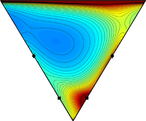In particular, the vorticity component $\omega _3^{*}$ (and the corresponding alignment $\omega _3^{*}/\omega$) is small along the right Vieillefosse tail where the RE system blows up, as shown in figure 4. The stabilizing effect of the rotation of the fluid element is exploited in reduced models for the velocity gradient dynamics to avoid the finite-time singularity thus producing steady-state statistics of the velocity gradient. Indeed, when the relative weight of the strain self-amplification $\alpha \lambda _i^2$ is reduced with respect to the magnitude of the rotation term $\beta (\omega -\omega _i^{*2})$, through the model coefficients $\alpha$ and $\beta$, then steady-state statistics can be obtained (Wilczek & Meneveau Reference Wilczek and Meneveau2014; Lawson & Dawson Reference Lawson and Dawson2015). This reduction of nonlinearity is attributed mainly to the pressure Hessian. On the other hand, the term $-\lambda _1^2$ has by definition a stabilizing effect on $\lambda _1$ while the corresponding vorticity contribution $(\omega ^2-\omega _1^{* 2})$ helps the growth of $\lambda _1$.

Since $-\lambda _3^2$ tends to make the dynamics unstable, it would be expected that, in order to prevent the velocity gradients becoming singular, the strongest effect of the pressure Hessian would be on $\lambda _3$. However, the average pressure Hessian contribution to $\lambda _3$, namely $\langle -H_{33}^{P*}\rangle$, is the smallest among the pressure components, although its variance is the largest, as shown in figure 1(b). Nevertheless, on average, this term does tend to hinder the growth of negative $\lambda _3$. The diagonal components of $\langle -H_{ij}^{P*}\rangle$, when normalized by $\tilde {\tau }^2$, do not show significant variations as a function of $\ell _F$. Therefore, at least on average, $H_{ij}^{P*}$ scales approximately as ${\sim }\tilde {\tau }^{-2}$, as expected from dimensional analysis, and consistent with models such as that of Wilczek & Meneveau (Reference Wilczek and Meneveau2014), which express the pressure Hessian as a linear combination of $\boldsymbol {S}\boldsymbol {\cdot }\boldsymbol {S}$ and $\boldsymbol {W}\boldsymbol {\cdot }\boldsymbol {W}^{\top }$. However, we would expect departures from this scaling for higher-order moments of $-H_{ij}^{P*}$ due to intermittency.

The average effect of the pressure Hessian on $\lambda _1$ is $\langle -H_{11}^{P*}\rangle$ and is positive, indicating that on average the pressure Hessian helps the growth of $\lambda _1$. This also implies that the pressure Hessian indirectly contributes to the stretching of $\boldsymbol {\omega }$ along $\boldsymbol {v}_1$, opposing the preferential alignment of the vorticity with the intermediate eigenvector $\boldsymbol {v}_2$. Interestingly, the largest average contribution from the pressure Hessian is for the intermediate eigenvalue, $\lambda _2$, and $\langle -H_{22}^{P*}\rangle$ is negative at all scales, driving $\lambda _2$ towards negative values. In this sense, the pressure Hessian hinders vortex stretching, suppressing the nonlinear amplification of $\omega _2^{*}$ through $\lambda _2$ (see (2.12)).

The viscous term $\langle H_{i(i)}^{\nu *}\rangle$ tends to hinder all the eigenvalues, with $\langle H_{11}^{\nu *}\rangle <0$, $\langle H_{22}^{\nu *}\rangle <0$ and $\langle H_{33}^{\nu *}\rangle >0$. In the dissipation range, $\langle H_{i(i)}^{\nu *}\rangle$ is largest in magnitude for $i=3$, which is associated with $\lambda _3$ having the largest magnitude on average. Furthermore, $\langle H^{\nu *}_{22}\rangle$ is very small compared to the other components, and therefore because of incompressibility, $\langle H_{11}^{\nu *}\rangle \approx -\langle H_{33}^{\nu *}\rangle$. The term is related to the curvature of the strain field and the clear tendency for $\langle H_{22}^{\nu *}\rangle$ to be small can be a consequence of the moderate fluctuations of the intermediate eigenvalue. Indeed, the contribution from $\lambda _2$ to the strain self-amplification, namely $\left \langle \lambda _2^3\right \rangle$, is the smallest among the contributions of the eigenvalues (Tsinober Reference Tsinober2001; Carbone & Bragg Reference Carbone and Bragg2020). Also, the sign of $\lambda _2$ fluctuates and the average $\lambda _2$ is small with respect to the average of the other eigenvalues. The average viscous stress components vary considerably across the scales, as expected since by definition these terms play a sub-leading dynamical role outside of the dissipation range.

The role of the sub-grid stress has not been investigated much in the literature, especially from the perspective of the strain-rate eigenframe. The sub-grid stress contribution to the dynamics increases with increasing $\ell _F$, and at the largest scales the sub-grid stress makes a leading order contribution to the eigenvalue dynamics. The sub-grid stress has strong variations across the scales even if normalized with a scale-dependent time scale. However, across all the scales $\langle H^{\tau *}_{11}\rangle$ remains very small compared to the other components and, as a consequence, $\langle H^{\tau *}_{33}\rangle \simeq \langle H^{\tau *}_{22}\rangle$. The sub-grid stress tends on average to drive $\lambda _2$ towards negative values and it hinders the growth of $|\lambda _3|$. In this sense, for the intermediate and most compressional principal directions, it acts similarly to the pressure Hessian, even if the quantitative trends of $H^{P*}_{i(i)}$ and $H^{\tau *}_{i(i)}$ across the scales are very different.

Figure 1(b) shows the variance of the contributions to the eigenvalue equation. The results show that the variance of $H_{i(i)}^{P*}$ is the largest of the contributions, with the variance of $H_{11}^{P*}$ and $H_{33}^{P*}$ decreasing as $\ell _F$ is increased, but becoming approximately constant in the inertial range when normalized by $\tilde {\tau }$. On the other hand, the variance of $H_{22}^{P*}$ is almost independent of $\ell _F$ when normalized by $\tilde {\tau }$, and this component is always the smallest. This is perhaps the reason why $\lambda _2$ undergoes smaller fluctuations in its time evolution than the other eigenvalues, which confirms the observation by Dresselhaus & Tabor (Reference Dresselhaus and Tabor1992) concerning the relatively small magnitude and persistency of the intermediate eigenvalue. The variance of the viscous term, normalized by $\tilde {\tau }$, becomes very small as $\ell _F$ is increased, decreasing as $\ell _F^{-\xi }$ with $\xi$ between 2 and 3.

Since there is a sign ambiguity in the definition of the eigenvectors $\boldsymbol {v}_i$, there is a corresponding ambiguity in the sign of $\omega ^*_i$. When solving (2.12) in a Lagrangian frame this ambiguity is removed through the choice of a particular direction for $\boldsymbol {v}_i$ in the initial conditions. However, we are computing terms based on data in the Eulerian frame (i.e. at fixed grid points). Therefore, instead of considering the dynamical contributions to (2.12), we will consider the dynamical contributions to the enstrophy equation (here we are calling $\omega _i^{*2} \equiv \omega _{(i)}^{*} \omega _i^{*}$ the enstrophy, although strictly speaking, the enstrophy is $\|\boldsymbol {\omega }\|^2=\sum _i \omega _i^{*2}$)

(4.2)\begin{equation} \tfrac{1}{2}D_t \omega_i^{*2} = \lambda_{(i)}\omega_i^{*2} - \varPi_{ij}^{*}\omega_j^{*}\omega_{(i)}^{*} + \varOmega_i^{\nu*}\omega_{(i)}^{*} - \varOmega_i^{\tau*}\omega_{(i)}^{*}. \end{equation}

In figure 2(a) we show the averages of the terms on the right-hand side of (4.2). The results show that the vortex-stretching term $\lambda _{(i)}\omega _i^{*2}$ acts on average to increase $\omega _1^{* 2}$ and $\omega _2^{* 2}$, and to reduce $\omega _3^{* 2}$. It is known that although $\boldsymbol {\omega }$ is preferentially aligned with $\boldsymbol {v}_2$ (Ashurst et al. Reference Ashurst, Kerstein, Kerr and Gibson1987; Meneveau Reference Meneveau2011), $\lambda _1\omega _1^{* 2}$ gives on average the largest contribution to vortex stretching $\langle \boldsymbol {\omega }^{\top }\boldsymbol {\cdot }\boldsymbol {S} \boldsymbol {\cdot } \boldsymbol {\omega }\rangle =\sum _{i}\langle \lambda _{(i)}\omega _i^{* 2}\rangle$ in the limit $\ell _F/\eta \to 0$ (i.e. for the unfiltered gradients) since $\lambda _1$ tends to be larger than $\lambda _2$ (Tsinober Reference Tsinober2001). Our results show that for $\ell _F$ outside of the dissipation range, the contribution to vortex stretching from $\lambda _1\omega _1^{* 2}$ becomes increasingly dominant, with $\langle \lambda _2\omega _2^{* 2}\rangle \ll \langle \lambda _1\omega _1^{* 2}\rangle$ in the inertial range. It is also interesting to note that while the normalized average $\tilde {\tau }^3\langle \lambda _{(i)}\omega _i^{* 2}\rangle$ changes substantially for $i=2$ as $\ell _F$ is increased from the dissipation to inertial range scales, it varies weakly with $\ell _F$ for $i=1,3$. This is in agreement with the weakening of the preferential alignment between the vorticity and the intermediate strain-rate eigenvector as $\ell _F$ is increased, while the statistical alignment of $\boldsymbol {\omega }$ with $\boldsymbol {v}_1$ and $\boldsymbol {v}_3$ depends very weakly on the filtering length (Danish & Meneveau Reference Danish and Meneveau2018).

Figure 2. (a) Average and (b) variance of the terms in (4.2), normalized by the scale-dependent time scale $\tilde {\tau }$, and plotted as a function of the filtering scale $\ell _F/\eta$. Different colours distinguish the various terms, while different line types and symbols refer to different components of those terms.

The alignment between the vorticity and the strain-rate eigenvectors is in part governed by the vorticity tilting term $\varPi _{ij}^{*}\omega _j^{*}$. That term plays a central role in determining the preferential alignment between $\boldsymbol {\omega }$ and $\boldsymbol {v}_2$ in the RE system, through $\varPi _{ij}^{RE*}\omega _j^{*}$, (Dresselhaus & Tabor Reference Dresselhaus and Tabor1992; Nomura & Post Reference Nomura and Post1998) and also in real turbulent flows due to the dominance of local over non-local contributions to the vorticity tilting (Lawson & Dawson Reference Lawson and Dawson2015). The vorticity tilting does not directly affect the total enstrophy $\|\boldsymbol {\omega }\|^2$, but it does contribute to the dynamics of the individual contributions $\omega _i^{*2}$. In particular, the results in figure 2 indicate that on average $\varPi _{ij}^{*}\omega _j^{*}\omega _{(i)}^{*}$ tends to enhance $\omega _3^{*2}$ while reducing $\omega _1^{*2}$. Therefore, the tilting tends to oppose the stretching of vorticity along $\boldsymbol {v}_1$ and to oppose the compression of vorticity along $\boldsymbol {v}_3$. In this sense, on average, $\varPi _{ij}^{*}\omega _j^{*}\omega _{(i)}^{*}$ has opposing effects to $\lambda _{(i)}\omega _i^{*2}$ for $i=1,3$. The results also show that the vorticity tilting makes a small positive contribution to the growth of $\omega _2^{*2}$ on average.

The viscous term acts on average to reduce the magnitude of all the components of enstrophy, with its effect strongest on $\omega _2^{* 2}$ and weakest on $\omega _3^{* 2}$. As expected, its average contribution markedly decreases with increasing filtering length as $\ell _F$ moves outside the dissipation range. The average sub-grid stress contribution to $D_t \omega _i^{*2}$ in (4.2) increases as $\ell _F$ is increased and becomes approximately constant in the inertial range when normalized by $\tilde {\tau }^3$, where its contribution becomes comparable in magnitude to the vortex-stretching terms $\lambda _i\omega _i^{*2}$, $i=2,3$. However, the sub-grid contribution is opposite in sign to the vortex-stretching contributions, tending to hinder $\omega _1^{*2}$ and $\omega _2^{*2}$ and to enhance $\omega _3^{*2}$.

The variances of the terms on the right-hand side of (4.2) are shown in figure 2(b). The variance of the vorticity tilting terms is very large, which indicates sudden rotations of the vorticity vector with respect to the eigenframe. Similar to the behaviour of the averages in figure 2(a), the results show that fluctuations in $\lambda _i\omega _i^{* 2}$ are greatest for $i=1$, and the contribution from $i=2$ becomes much smaller than that from $i=1$ for $\ell _F$ in the inertial range. Most interestingly, we find that the sub-grid contributions for $i=1,2$ are very similar (almost identical in the inertial range), while the contribution for $i=3$ is much smaller, a feature preserved across the scales. This indicates that there is not a simple relationship between the sub-grid and vortex-stretching terms, which poses a challenge for large-eddy simulation modelling.

We have computed the moments in figures 1 and 2 across a range of Reynolds numbers (particular case of $Re_{\lambda } = 224$ shown in appendix D) and obtained similar trends. This confirms that the statistics are converged and show that the moments depend weakly on the Reynolds number, at least in the range considered ($Re_{\lambda } \approx 200\text {--}600$). This is not too surprising given that these are normalized lower-order moments, but we would expect stronger Reynolds number effects for higher-order moments, due to intermittency.

4.2. Behaviour of eigenvalues and vorticity in the $R$, $Q$ plane

The statistical behaviour in the $R,Q$ plane, expressed in terms of the joint PDF of the invariants, is captured qualitatively by most of the models. The agreement between models and DNS is particularly good in closures based on tensor representations of the pressure Hessian in terms of the local velocity gradients squared (Wilczek & Meneveau Reference Wilczek and Meneveau2014) and closures which include multiscale energy transfer (Biferale et al. Reference Biferale, Chevillard, Meneveau and Toschi2007; Johnson & Meneveau Reference Johnson and Meneveau2017). However, the Gaussian closure underpredicts the probability along the left Vieillefosse tail, while it overestimates the probability of states along the right Vieillefosse tail and of vorticity-dominated states. Models based on the recent fluid deformation (RFD) hypotheses (Chevillard & Meneveau Reference Chevillard and Meneveau2006) considerably underestimate the probability of large values for $R,Q$. This issue also persists in more sophisticated closures in which the velocity field is supposed to be Gaussian at some time in the past (Johnson & Meneveau Reference Johnson and Meneveau2016) or in which multifractality of the gradient statistics is imposed (Pereira et al. Reference Pereira, Moriconi and Chevillard2018). To further our understanding of the eigenvalue and vorticity dynamics, we now show the average of the eigenvalues and eigenframe vorticity components in the phase space of the velocity gradient invariants.

In figure 3, we show the average of the filtered strain-rate eigenvalues conditioned on the principal invariants of the filtered velocity gradient $\langle \tilde {\tau }\lambda _i| {\tilde {\tau }}^3 R, {\tilde {\tau }}^2 Q\rangle$, where $R=-\textrm {Tr}(\boldsymbol {A}^3)/3$ and $Q=-\textrm {Tr}(\boldsymbol {A}^2)/2$. The colour map is in a linear scale, and the results refer to the filtering lengths $\ell _F/\eta =7.0$ and $\ell _F/\eta =67.3$. The colour bar range has been truncated in order to highlight the trend of the variables around the most probable values. The results show that $\left \langle \lambda _2|R,Q\right \rangle$ is relatively large and positive along the right Vieillefosse tail compared to its value in other regions of the phase space. Since the joint PDF of $R,Q$ is large along the right Vieillefosse tail (Chong et al. Reference Chong, Soria, Perry, Chacin, Cantwell and Na1998; Lüthi, Holzner & Tsinober Reference Lüthi, Holzner and Tsinober2009; Elsinga & Marusic Reference Elsinga and Marusic2010; Meneveau Reference Meneveau2011) then that phase space region contributes strongly to the tendency for $\lambda _2$ to be positive, with $\left \langle \lambda _2\right \rangle >0$. In contrast, $\left \langle \lambda _1 | R,Q\right \rangle$ is relatively small along the right Vieillefosse tail as compared to the larger value it takes along the left Vieillefosse tail, where $R<0$, corresponding to states of biaxial compression with $\lambda _2<0$. The most compressional eigenvalue $\left \langle \lambda _3|R,Q\right \rangle$ tends to have relatively small magnitudes in the vortex-stretching quadrant ($Q>0$ and $R<0$), compared to values it takes on other regions of the $R,Q$ plane. On the other hand, $\left \langle \lambda _2|R,Q\right \rangle$ is positive on average here, showing that it contributes to the stretching of vorticity along the direction $\boldsymbol {v}_2$ in this quadrant.

Figure 3. Average of the filtered strain-rate eigenvalues conditioned on the second and third principal invariants of the filtered velocity gradient tensor. Panels (a–c) show conditional averages $\langle \tilde {\tau }\lambda _{1}|{\tilde {\tau }}^3 R, {\tilde {\tau }}^2 Q\rangle$, $\langle \tilde {\tau }\lambda _{2}|{\tilde {\tau }}^3 R, {\tilde {\tau }}^2 Q\rangle$ and $\langle \tilde {\tau }\lambda _{3}|{\tilde {\tau }}^3 R, {\tilde {\tau }}^2 Q\rangle$, respectively, for $\ell _F/\eta =7.0$ and (d–f) show the corresponding quantities for $\ell _F/\eta =67.3$. The colour map is in linear scale, and the thick black lines represent the Vieillefosse tails. Note that average values greater/smaller than the largest/smallest value in the colour bar are clipped to the colour corresponding to largest/smallest value in the colour bar.

In figure 4, we show the results for $\left \langle (\tilde {\tau }\omega _i^{*})^2|{\tilde {\tau }}^3 R, {\tilde {\tau }}^2 Q\right \rangle$, for the same filtering lengths $\ell _F/\eta =7.0$ and $\ell _F/\eta =67.3$. The quantity $\omega _i^{*2}$ rather than $\omega _i^{*}$ has been employed to remove the ambiguity of the sign of $\omega _i^{*}$ that was discussed earlier, and the colour map is in logarithmic scale. The quantity $\left \langle \omega _2^{*2}|R,Q\right \rangle$ is large over a wide region of the upper plane $Q>0$ where rotational motion dominates the velocity gradients. It also takes relatively large values close to the right Vieillefosse tail, compared to the values that the other vorticity components take in that region. The results for $\left \langle \omega _3^{*2}|R,Q\right \rangle$ indicate that the vorticity component along $\boldsymbol {v}_3$ is smaller below and in the proximity of the right Vieillefosse tail compared to other regions of the phase space and is associated with the misalignment between $\boldsymbol {\omega }$ and $\boldsymbol {v}_3$ in that region of the $R,Q$ plane (Carbone et al. Reference Carbone, Iovieno and Bragg2020). This can be related to the compression along the vorticity axis that arises due to incompressibility of the flow, described by the second term on the right-hand side of (2.10b) together with the local pressure Hessian contribution. Since this term is non-negative, then it acts to suppress the growth of the compressional eigenvalue $\lambda _3$. However, if the vorticity was perfectly aligned with $\boldsymbol {v}_3$ then this term would vanish. Therefore, misalignment of the vorticity with $\boldsymbol {v}_3$ stabilizes the system by providing a mechanism to prevent the blow-up of $\lambda _3$ along the right Vieillefosse tail. The relatively large value of $\left \langle \omega _3^{*2}|R,Q\right \rangle$ observed in the quadrant $R>0$ and $Q>0$ compared to other quadrants is expected, since this is the quadrant associated with vortex compression (Tsinober Reference Tsinober2001).

Figure 4. Average of the square of the vorticity components conditioned on the second and third principal invariants of the filtered velocity gradient tensor. Panels (a–c) show conditional averages $\left \langle (\tilde {\tau }\omega _1^{*})^2|{\tilde {\tau }}^3 R, {\tilde {\tau }}^2 Q\right \rangle$, $\left \langle (\tilde {\tau }\omega _2^{*})^2|{\tilde {\tau }}^3 R, {\tilde {\tau }}^2 Q\right \rangle$ and $\left \langle (\tilde {\tau }\omega _3^{*})^2|{\tilde {\tau }}^3 R, {\tilde {\tau }}^2 Q\right \rangle$, respectively, for $\ell _F/\eta =7.0$ and (d–f) show the corresponding quantities at $\ell _F/\eta =67.3$. The colour map is in $\log _{10}$ scale and the thick black lines represent the Vieillefosse tails. Note that average values greater/smaller than the largest/smallest value in the colour bar are clipped to the colour corresponding to largest/smallest value in the colour bar.

The conditional averages shown in figures 3 and 4 confirm that, qualitatively, the statistics are weakly dependent on the filtering length scale, as observed for the probability density flux in the $R,Q$ plane (Danish & Meneveau Reference Danish and Meneveau2018). One exception is the behaviour of $\omega _2^{*}$, for which comparing figures 4(b) and 4(e) reveals significant qualitative changes in the behaviour of $\left \langle \omega _2^{*2}|R,Q\right \rangle$ as $\ell _F$ is increased.

4.3. Rotation of the strain-rate eigenframe and tilting of the vorticity vector

The tilting of the vorticity vector with respect to the strain-rate eigenframe plays a central role in determining the geometric alignments of the strain rate and vorticity, and the rotation rate of the eigenframe can take on very large values even in simple flows (Dresselhaus & Tabor Reference Dresselhaus and Tabor1992). This rotation rate is determined by the interaction between vorticity, pressure gradient and viscous and sub-grid forces, and (2.10c) suggests that the rotation can be very strong when the differences between the strain-rate eigenvalues becomes small. To understand this better, and the effect of filtering on these processes, we now turn to analyse in detail the statistics of the rotation rate of the eigenframe and its dependence upon the local state of the velocity gradient.

Figure 5(a–c) shows the second moment of the different contributions to the eigenframe rotation rate $\varPi _{ij}^*$ (see (2.14)), and figure 5(d–f) shows the PDF of the square of the difference in the eigenvalues, which represents the resistance of the eigenframe (Vieillefosse Reference Vieillefosse1982). While the local contributions (captured by the RE model) to the eigenframe rotation rate have been investigated in detail (Dresselhaus & Tabor Reference Dresselhaus and Tabor1992), together with its impact on the vorticity dynamics, the non-local contributions have received less attention. The second moment of the pressure Hessian contribution is close to the second moment of the overall rotation rate and they are almost independent of the filtering length (when normalized by $\tilde {\tau }$). This indicates that the non-local effects on the rotation rate of the eigenframe dominate over the contribution from vorticity that features in the RE model. However, we will observe that the local RE term plays a leading role in the tilting of the vorticity vector. The sub-grid stress also gives an important contribution to the eigenframe rotation rate, especially at large scales. On the other hand, the viscous contribution is small with $\left \langle (\tilde {\tau } \varPi _{ij}^{\nu *})^2 \right \rangle$ decreasing as $\ell _F^{-\xi }$, with $\xi$ between 2 and 3. The component $\left \langle (\tilde {\tau } \varPi _{31}^{*})^2 \right \rangle$, associated with the angular velocity of the eigenframe along $\boldsymbol {v}_2$, is much smaller than the other components. If we consider the PDFs of $(\lambda _j-\lambda _i)^2$ in figure 5(d–f) we see that the mode of the random variable is considerably larger for $(\lambda _1-\lambda _3)^2$ than for the other cases. The reason for this is that due to incompressibility, $(\lambda _1-\lambda _3)^2\to 0$ also implies $\lambda _2\to 0$, and the probability of states with strain rate almost zero is vanishingly small. As a result, the average values of $(\lambda _1-\lambda _3)^2$ are larger than for $(\lambda _2-\lambda _3)^2$ or $(\lambda _1-\lambda _2)^2$, implying on average an increased resistance to rotations of the eigenframe about $\boldsymbol {v}_2$, and hence to $\left \langle (\tilde {\tau } \varPi _{31}^{*})^2 \right \rangle$ being smaller than the other components.

Figure 5. (a–c) Second moment of the components of the RE, pressure, viscous and sub-grid contributions to the strain-rate eigenframe rotation rate, together with the overall rotation rate. (d–f) The PDF of the square of the differences in the eigenvalues, which appear in the equation for the rotation rate of the eigenframe (2.10c).

The results in figure 5(d–f) also indicate that the probability of axisymmetric states with $\lambda _2\approx \lambda _1$ and $\lambda _2\approx \lambda _3$ is quite high, with the probability of observing $\lambda _2\approx \lambda _1$ larger, in agreement with previous results that showed that axisymmetric extension occurs more often than axisymmetric compression (Lund & Rogers Reference Lund and Rogers1994; Meneveau Reference Meneveau2011). However, the probability to observe $\tilde {\tau }(\lambda _2-\lambda _3)\to 0$ is only three times smaller than that for observing $\tilde {\tau }(\lambda _2-\lambda _1)\to 0$. A more accurate estimation of the relative occurrence rates of axisymmetric compression and expansion can be achieved by means of a dimensionless parameter (Lund & Rogers Reference Lund and Rogers1994) as discussed in § 4.4.2. The main effect of filtering on these PDFs is to simply suppress the tails, associated with reduced intermittency at larger scales. However, for the PDF of $(\lambda _1-\lambda _3)^2$, there is also a significant effect of filtering on the behaviour for $(\lambda _1-\lambda _3)^2\to 0$, with the probability of states with $(\lambda _1-\lambda _3)^2\to 0$ decreasing as $\ell _F$ is increased.

The quantity $\lambda _j-\lambda _i$ acts as a weight in (2.10c), and the behaviour of $\varPi _{ij}^{*}$ depends on how the various contributions to $\varPi _{ij}^{*}$ on the right-hand side of (2.10c) behave as $\lambda _j-\lambda _i$ varies. To explore this, in figure 6 we show results for $\left \langle X _{ij}^2\vert \lambda _j-\lambda _i \right \rangle$, with $i>j$ such that $\lambda _j-\lambda _i > 0$, where $X_{ij}$ is either the eigenframe rotation rate $\varPi _{ij}^*$ or else one of the distinct contributions to $\varPi _{ij}^*$, namely $\varPi ^{RE*}_{ij}, \varPi ^{P*}_{ij}, \varPi ^{\nu *}_{ij} or \varPi ^{\tau *}_{ij}$ (see (2.14)). The results show that $\left \langle X _{ij}^2\vert \lambda _j-\lambda _i \right \rangle \propto (\lambda _j-\lambda _i)^{-2}$ for small $\tilde {\tau }(\lambda _j-\lambda _i)$, indicating a weak correlation between $(\lambda _j-\lambda _i)$ and the vorticity, pressure Hessian, sub-grid stress and viscous stress in this range. However, for $\tilde {\tau }(\lambda _j-\lambda _i)\geq O(1)$, $\left \langle X ^2\vert \lambda _j-\lambda _i \right \rangle$ starts to increase for some of the cases. This non-monotonic behaviour is quite intriguing, but the increase cannot persist in the limit $\tilde {\tau }(\lambda _j-\lambda _i)\to \infty$ if the flow field is to remain regular. Also, the results show that the increase at $\tilde {\tau }(\lambda _j-\lambda _i)\geq O(1)$ becomes less apparent as the filter length is increased. For the smallest filter scales, the results in figure 6 show that the dominant contribution to the eigenframe rotation-rate comes from the pressure Hessian, with important contributions from the sub-grid stress and RE term associated with vorticity in some cases (e.g. especially for $i=2,j=1$). At larger scales, however, the sub-grid term makes a strong contribution, similar in size to that from the pressure Hessian with the RE playing a smaller role. The viscous contribution is small at all scales and for all components.

Figure 6. Second moment of the contributions to the eigenframe rotation rate conditioned on the difference in the eigenvalues. Panels (a,c,e) correspond to $\ell _F/\eta = 7.0$ and (b,d,f) to $\ell _F/\eta = 209.4$.

The rotation rate of the eigenframe plays an important role in the vorticity dynamics through the vortex tilting mechanism, described by the term $\varPi _{ij}^{*}\omega _j^{*}$ in (2.12). The second moment of $\varPi _{ij}^{*}\omega _j^{*}$ and the various contributions to it are shown in figure 7(a–c) together with the PDFs of $|\varPi _{ij}^{*}\omega _j^{*}|$ in figure 7(d–f). The RE and pressure Hessian contributions to $\langle (\varPi _{ij}^{*}\omega _j^{*})^2\rangle$ are the largest and are similar in size, showing that the local (i.e. that captured by the RE model) and non-local contributions to $\langle (\varPi _{ij}^{*}\omega _j^{*})^2\rangle$ are similar. The reason why the RE term makes a significant contribution to the vorticity tilting that is similar to that of the pressure Hessian, despite the fact that the former gives a much smaller contribution to the eigenframe rotation rate, could be related to the weak preferential alignment between the vorticity and the pressure Hessian (Carbone et al. Reference Carbone, Iovieno and Bragg2020). The viscous contribution is small over the range of $\ell _F$ considered, with $\langle (\tilde {\tau }\varPi _{ij}^{\nu *}\omega _j^{*})^2\rangle$ decreasing as $\ell _F^{-\xi }$, with $\xi$ between 2 and 3. The vorticity tilting about axis $\boldsymbol {v}_2$ is slightly larger than the tilting about the other two axes, in contrast to the reduced eigenframe rotation rate about axis $\boldsymbol {v}_2$ shown in figure 5. However, the difference between the components of $\langle (\varPi _{ij}^{*}\omega _j^{*})^2\rangle$ is smaller than the difference between the components of $\langle (\varPi _{ij}^{*})^2\rangle$ shown in figure 5.

Figure 7. (a–c) Second moment of the RE, pressure, viscous and sub-grid contributions to the vorticity tilting term, together with the second moment of the total vorticity tilting term. (d–f) The PDF of the vorticity tilting term in (2.12).

The PDFs of $|\varPi _{ij}^{*}\omega _j^{*}|$ are shown in figure 7(d–f), revealing wide power-law tails and large values of vorticity tilting. Quite remarkably, the PDFs are almost insensitive to the filtering scale $\ell _F$, such that very strong vorticity tilting resulting in highly non-Gaussian behaviour is a feature that persists beyond just the dissipation range. This intermittent behaviour, however, is probably kinematic rather than purely dynamical in origin. In particular, (2.10c) shows that $\varPi _{ij}^{*}$ depends on $(\lambda _j-\lambda _i)^{-1}$, such that small values of $\tilde {\tau }(\lambda _j-\lambda _i)$, which occur with high probability, can lead to large values of $\tilde {\tau }^2\varPi _{ij}^{*} \omega _j^{*}$.

A peculiar situation to consider is when two eigenvalues intersect ($\lambda _i = \lambda _j$), which may result in a very large rotation rate of the eigenvectors. Indeed, in that situation, the directions of two of the strain-rate eigenvectors associated with the coincident eigenvalues are not well defined. All vectors belonging to the plane orthogonal to the eigenvector associated with the other (distinct) eigenvalues are strain-rate eigenvectors. Therefore, the orientation of those eigenvalues can be chosen on the plane orthogonal to the eigenvector associated with the other (distinct) eigenvalues and there is some arbitrariness in the projection of the equations for the gradient into the eigenframe. In the simple RE system, the eigenvalues cannot intersect and the components of the vorticity in the strain-rate eigenframe cannot change sign. This is due to the several conservation laws in the RE system, in particular the determinant of the commutator between the symmetric and anti-symmetric parts of the velocity gradient is a first integral of the RE system (Vieillefosse Reference Vieillefosse1982). The pressure Hessian and viscous stress are key to weakening those constraints and reducing the number of first integrals thus avoiding finite-time singularities. Although our results in figure 5(d–f) show significant probability for $(\lambda _i-\lambda _j)\to 0$, we cannot provide conclusive evidence that eigenvalues can intersect. For this, we would need to track the non-ordered eigenvalues of fluid particles in the Lagrangian frame and look for evidence that their ordering changes along the trajectory. This interesting problem is left for future investigations.

4.4. Characterizing the pressure Hessian

In figure 8(a,c,e) we show the PDFs of the diagonal components of the pressure Hessian in the eigenframe, filtered at various scales. The PDFs show wide tails for the smallest filtering lengths $\ell _F$, consistent with the observation of highly intermittent acceleration statistics in turbulence (Ayyalasomayajula, Warhaft & Collins Reference Ayyalasomayajula, Warhaft and Collins2008), but the extreme events become much rarer as $\ell _F$ is increased, with the PDFs approaching a Gaussian shape at the largest scales. The PDFs are also strongly positively skewed, with the skewness decreasing as $\ell _F$ is increased. The local/isotropic part of the unfiltered pressure Hessian is proportional to the second unfiltered invariant

(4.3)\begin{equation} Q=\|\boldsymbol{\omega}\|^2/4 - \|\boldsymbol{S}\|^2/2, \end{equation}

and since the PDF of $Q$ is positively skewed (Meneveau Reference Meneveau2011), so also will be the PDF of the local part of the pressure Hessian. The dependence of the non-local contribution to the pressure Hessian on the local properties of $Q$ is more complicated. However, we note that during large events where $Q\gg \tau _{\eta }^2$, the local part of the pressure Hessian is expected to dominate over the non-local part (see below), since extreme events in $Q$ are spatially localized. For the filtered fields, there is an additional contribution to the isotropic part of the filtered pressure Hessian since $\textrm{Tr}(\widetilde{{\boldsymbol{H}^P}}+\widetilde{{\boldsymbol{A}}}^2 + {\boldsymbol{H}}^\tau)=0$.

Figure 8. The PDF of the diagonal components of the pressure Hessian in the eigenframe normalized using scale-dependent time scale $\tilde {\tau }$. Panels (a,c,e) show results for the full pressure Hessian, and (b,d,f) are for the anisotropic part of the pressure Hessian.

4.4.1. Characterizing the anisotropic pressure Hessian

The anisotropic pressure Hessian is defined as

(4.4)\begin{equation} \overline{H}_{ij}^{{{{P}*}}} \equiv H_{ij}^{P*} - \tfrac{1}{3}H_{kk}^{P*}\delta_{ij} \end{equation}

and the PDFs of the diagonal components $\overline{H}_{i(i)}^{{{{P}*}}}$ are shown in figure 8(b,d,f), for various $\ell _F$. Comparing these results to those in figure 8(a,c,e) reveals that the strong positive skewness of the PDF of the full pressure Hessian arises from the dominating contribution of the local pressure Hessian during large events. Indeed, the PDF of $\overline{H}_{22}^{{{{P}*}}}$ is negatively skewed, indicating that the strongest fluctuations in $\overline{H}_{22}^{{{{P}*}}}$ tend to help the growth of $\lambda _2$ (since $H_{i(i)}^{P *}$ appears with a minus sign in (2.10b)) and hence also vortex stretching. This is in contrast with the average negative value of $-H_{22}^{P*}$ observed in figure 1.

In order to understand more fully the relationship between ${\overline{H}_{i(i)}^{{{{P}*}}}}$ and the local properties of the flow, in figure 9(a,c,e), we consider the results for $\langle \overline{H}_{i(i)}^{{{{P}*}}}|\lambda _i^2\rangle$ as a function of the filtering scale. For $i=1$, this quantity is always negative, and since the pressure Hessian appears with a negative sign in front of it in the eigenvalue equation (2.10b), this indicates that on average $\overline{H}_{11}^{{{{P}*}}}$ acts to amplify $\lambda _1$, for all values of $\lambda _1^2$. For $\tilde {\tau }\lambda _1\leq O(1)$, $\langle \overline{H}_{11}^{{{{P}*}}}|\lambda _1^2\rangle$ becomes increasingly negative with increasing $\lambda _1^2$, varying almost linearly with $\lambda _1^2$. The contribution to $\lambda _2$, namely $\langle \overline{H}_{22}^{{{{P}*}}}|\lambda _2^2\rangle$, is always positive and therefore on average $\overline{H}_{22}^{{{{P}*}}}$ hinders the growth of positive $\lambda _2$ for all values of $\lambda _2^2$. Furthermore, for $\tilde {\tau }|\lambda _2| \leq O(1)$, $\langle \overline{H}_{22}^{{{{P}*}}}|\lambda _2^2\rangle$ increases almost linearly with increasing $\lambda _2^2$ except for the larger filter scales, for which a nonlinear behaviour is apparent even for $\tilde {\tau }|\lambda _2|\ll 1$. The behaviour of $\langle \overline{H}_{33}^{{{{P}*}}}|\lambda _3^2 \rangle$ is quite peculiar, showing that on average $\overline{H}_{33}^{{{{P}*}}}$ amplifies $\lambda _3$ (increases $|\lambda _3|$) for very small $\tilde {\tau }\lambda _3$, but then hinders its growth outside of this regime. The range of $\tilde {\tau }\lambda _3$ over which $\overline{H}_{33}^{{{{P}*}}}$ amplifies $\lambda _3$ on average decreases with increasing filter scale.

Figure 9. Average of the diagonal components of the anisotropic pressure Hessian in the eigenframe conditioned on (a,c,e) the corresponding eigenvalues squared, and (b,d,f) the corresponding vorticity components squared. Insets highlight the results for small values of $\tilde {\tau }^2 {\lambda _i}^2$ and $\tilde {\tau }^2 {\omega _i^{*}}^2$.

Over the entire range of $\tilde {\tau }\lambda _i$ shown, the effect of filtering appears quite weak (it is more apparent for $i=2$ since in that case the results extend over a smaller region of $\tilde {\tau }\lambda _i$ owing to the smaller fluctuations of $\lambda _2$ compares with $\lambda _1$ or $\lambda _3$). Nevertheless, the insets to figure 9(a,c,e) highlight that for $(\tilde {\tau }\lambda _i)^2\leq 0.3$, filtering reduces the magnitude of both $\langle \tilde {\tau }^2\overline{H}_{11}^{{{{P}*}}}|\lambda _1^2\rangle$ and $\langle \tilde {\tau }^2\overline{H}_{22}^{{{{P}*}}}|\lambda _3^2\rangle$, whereas the magnitude of $\langle \tilde {\tau }^2\overline{H}_{33}^{{{{P}*}}}|\lambda _3^2\rangle$ is reduced by filtering in the regime where it is positive, but increased in the region where it is negative.

In figure 9(b,d,f), we consider the results for $\langle \overline{H}_{i(i)}^{{{{P}*}}}|\omega _i^{*2}\rangle$. For $\tilde {\tau }^2\omega _i^{*2}\gtrsim 3$, $\langle \overline{H}_{i(i)}^{{{{P}*}}}|\omega _i^{*2}\rangle$ is negative, leading to the amplification of $\lambda _1$ and positive $\lambda _2$, but the suppression of $|\lambda _3|$. In this regime, $\langle \overline{H}_{i(i)}^{{{{P}*}}}|\omega _i^{*2}\rangle \propto \omega _i^{*2}$ is a good approximation. For $\tilde {\tau }^2\omega _i^{*2}<3$, however, $\langle \overline{H}_{i(i)}^{{{{P}*}}}|\omega _i^{*2}\rangle$ changes sign for $i=2,3$ and has a highly nonlinear behaviour, similar to that of $\langle \overline{H}_{33}^{{{{P}*}}}|\lambda _3^2\rangle$. Taken altogether, the results in figure 9 indicate that closures such as the tetrad model (Chertkov et al. Reference Chertkov, Pumir and Shraiman1999; Naso & Pumir Reference Naso and Pumir2005) and enhanced Gaussian closure (Wilczek & Meneveau Reference Wilczek and Meneveau2014) which predict that the anisotropic pressure Hessian depends on the square of the local velocity gradient are able to capture several important features, but not all, especially in the regime of small gradients.

In figure 10, we show results for the first and second moments of $\overline{H}_{i(i)}^{{{{P}*}}}$ conditioned on the isotropic part of the pressure Hessian, $H_{kk}^{P*}/3 = 2Q/3$ (with little abuse of notation in the filtered case, in which Q denotes $-\widetilde{{\boldsymbol{A}}^2}/2$). The results show that $\langle \overline{H}_{i(i)}^{{{{P}*}}}|2Q/3\rangle$ varies almost linearly with $Q$, but with different slopes for $Q>0$ and $Q<0$. This provides some support for closure models that assume a linear relationship between the anisotropic pressure Hessian and $Q$ (Chevillard & Meneveau Reference Chevillard and Meneveau2006; Chevillard et al. Reference Chevillard, Meneveau, Biferale and Toschi2008; Wilczek & Meneveau Reference Wilczek and Meneveau2014). However, whether such models correctly describe the change in slope around $Q=0$ should be considered in future work. Also, the DNS results indicate that the average of the norm squared of the anisotropic pressure Hessian conditioned on the invariant $Q$ approximately scales as $|Q|$ (Chevillard et al. Reference Chevillard, Meneveau, Biferale and Toschi2008), while it scales as $Q^2$, by construction, in models that assume a linear relationship between the anisotropic pressure Hessian and $Q$.

Figure 10. (a,c,e) Average and (b,d,f) second moment of the diagonal components of the anisotropic pressure Hessian conditioned on the isotropic part of the filtered pressure Hessian (which is equal to $2/3$ times the second principal invariant of the velocity gradient $Q$), for various filtering lengths $\ell _F/\eta$. Insets in (a,c,e) highlight the results for small values of $2\tilde {\tau }^2 Q/3$.

The second invariant $Q$ is a measure of the relative importance of strain and vorticity at a given point in the flow. The results in figure 10(a,c,e) indicate that on average $\overline{H}_{11}^{{{{P}*}}}$ aids the growth of $\lambda _1$ in strain-dominated regions, but counteracts the growth of $\lambda _1$ in vorticity-dominated regions. The average and the variance of the contribution from $\overline{H}_{11}^{{{{P}*}}}$ is small compared to the contributions from the other diagonal components, in contrast to what was observed earlier for the full component $H_{11}^{P*}$. This differing behaviour is due to the contribution of the isotropic pressure Hessian that is proportional to $Q$. In vorticity-dominated regions, the average contribution from $\overline{H}_{22}^{{{{P}*}}}$ becomes increasingly negative with increasing $Q$, and it therefore helps the growth of positive $\lambda _2$. This opposes the local part of the pressure Hessian that acts to reduce positive $\lambda _2$ events in vorticity-dominated regions. The third diagonal component $\overline{H}_{33}^{{{{P}*}}}$ counteracts the growth of $|\lambda _3|$ in strain-dominated regions, which is critical to stabilize the dynamics. This feature is absent in the RE model where $\overline{H}_{ij}^{{{{P}*}}}=0$, which is one reason that system blows up.

The results in figure 10(b,d,f) for $\langle \overline{H}_{i(i)}^{{{{{P}*}}}^{2}}|2Q/3\rangle$, together with the insets of figure 10(a,c,e), show that the effect of $\overline{H}_{i(i)}^{{{{P}*}}}$ on the eigenframe dynamics does not vanish when $Q\to 0$, which was also observed in Chevillard et al. (Reference Chevillard, Meneveau, Biferale and Toschi2008), and is something that is not captured by closure models such as the tetrad model (Chertkov et al. Reference Chertkov, Pumir and Shraiman1999), the Lagrangian linear diffusion model (Jeong & Girimaji Reference Jeong and Girimaji2003) or the recent fluid deformation approximation (Chevillard & Meneveau Reference Chevillard and Meneveau2006). Moreover, the peculiar behaviour of the anisotropic pressure Hessian components observed in figure 9 for small $\tilde {\tau }\lambda _i$ and $\tilde {\tau }\omega _i$ translates into a non-trivial and non-monotonic behaviour of the pressure Hessian components at small $Q$, as shown in the insets of figure 10.

4.4.2. Preferential states of the pressure Hessian

We now turn to characterizing the state of the anisotropic pressure Hessian ${\boldsymbol {\overline {H}}^{{{{P}}}}}$ by means of its eigenvalues $\bar {\phi }_i$, which are associated with its eigenvectors $\boldsymbol {w}_i$. The eigenvalues of the full pressure Hessian are denoted by $\phi _i$. The shape of the anisotropic part of the pressure Hessian can be quantified by means of the dimensionless quantity

(4.5)\begin{equation} s^* = -\sqrt{6}\frac{\textrm{Tr}[(\overline{\boldsymbol{H}}^{{{{P}}}})^3]} {\left(\textrm{Tr}[(\overline{\boldsymbol{H}}^{{{{P}}}})^2]\right)^{3/2}} = -\frac{3\sqrt{6} \quad \bar{\phi}_1\bar{\phi}_2\bar{\phi}_3} {(\bar{\phi}_1^2+\bar{\phi}_2^2+\bar{\phi}_3^2)^{3/2}}. \end{equation}

The variable $s^*$ has been proposed in Lund & Rogers (Reference Lund and Rogers1994), and since only $\bar {\phi }_2$ is not sign definite, the sign of $s^*$ is determined by the sign of $\bar {\phi }_2$, and the PDF of $s^*$ can be used to quantify the probability of the tensor being found in axisymmetric states. The PDF of $s^*$ is shown in figure 11(a), and the results show that $s^*$ is preferentially positive, indicating that $\bar {\phi }_2$ is also preferentially positive. As $\ell _F$ is increased, the PDF tends to the constant value of $1/2$, corresponding to a uniform random variable (Lund & Rogers Reference Lund and Rogers1994). The preference for positive values of $s^*$ indicates that the anisotropic pressure Hessian exhibits a preference to stretch fluid elements along the direction $\boldsymbol {w}_3$ (since $-\boldsymbol {H}^P$ appears in (2.4)), and to compress them in the plane spanned by $\boldsymbol {w}_1$ and $\boldsymbol {w}_2$, that is orthogonal to $\boldsymbol {w}_3$. In figure 11(b) we show the corresponding results for the strain-rate tensor, for which $s^* = -\sqrt {6}\textrm {Tr}[\boldsymbol {S}^3]/ (\textrm {Tr}[\boldsymbol {S}^2])^{3/2}$. The results for this quantity in figure 11(b) show that the preference for $\boldsymbol {S}$ to be in a state of bi-axial extension is much greater than that for $\boldsymbol {\overline {H}}^{{{{P}}}}$, though in both cases, this preference for bi-axial extension generally becomes weaker as $\ell _F$ is increased.

Figure 11. The PDF of $s^*$ for (a) the anisotropic pressure Hessian, and (b) the strain rate. Dashed lines indicate the probability distribution for a random uncorrelated field.

In order to gain further insight into the state of the full pressure Hessian $\boldsymbol {{H}}^P$, we aim to characterize the full space of the independent dimensionless quantities that can be formed using the invariants of $\boldsymbol {{H}}^P$. Since $\boldsymbol {{H}}^P$ is symmetric with three real, independent eigenvalues, two dimensionless quantities can be defined. In the context of the Reynolds stresses, the Lumley triangle provides an insightful way to characterize its anisotropic properties (Lumley Reference Lumley1979; Pope Reference Pope2000). However, this cannot be applied to $\boldsymbol {{H}}^P$ since it is not positive definite. As an alternative, we seek to construct an invariant triangle, analogous to the Lumley triangle, by employing the invariants of the normalized quantity

(4.6)\begin{equation} b_{ij} = \frac{H_{ij}^P-H_{kk}^P\delta_{ij}/3}{\sqrt{H^P_{mn}H^P_{mn}}}, \end{equation}

which simply corresponds to the normalized components of the anisotropic pressure Hessian. The first two invariants of $\boldsymbol {b}$ are $\textrm {Tr}(\boldsymbol {b})=0$ and

(4.7)\begin{equation} b^2 \equiv \textrm{Tr}(\boldsymbol{b}^2) = 1-\left(\frac{H_{kk}^P}{\sqrt{3H_{ij}^PH_{ij}^P}}\right)^2. \end{equation}

Therefore $b^2$ is bounded, $b^2\in [0,1]$. Moreover, the second invariant of $\boldsymbol {b}$ is related to the quantity $D^*$ through $b^2 = 1-(D^*)^2$, where

(4.8)\begin{equation} D^* = -\frac{\textrm{Tr}[(\boldsymbol{H}^P)]}{\sqrt{3\textrm{Tr}[(\boldsymbol{H}^P)]^2)}} = -\frac{\phi_1+\phi_2+\phi_3}{ \sqrt{3}\left( \phi_1^2+\phi_2^2+\phi_3^2\right)^{1/2} }. \end{equation}

The parameter $D^*$ was proposed in Lund & Rogers (Reference Lund and Rogers1994) to quantify the relative magnitude of the isotropic dilatation/compression of a tensor. The constraint on the third invariant is obtained through the discriminant of the characteristic equation of $\boldsymbol {b}$. Since the eigenvalues of $\boldsymbol {b}$ are real, it follows that

(4.9)\begin{equation} \varDelta = \tfrac{1}{2}(\textrm{Tr}(\boldsymbol{b}^2))^3 - 3(\textrm{Tr}(\boldsymbol{b}^3))^2 \ge 0, \end{equation}

and hence $| {\sqrt {6} \textrm {Tr}(\boldsymbol {b}^3)} | \le (\textrm {Tr}(\boldsymbol {b}^2))^{3/2}$. The zero discriminant case corresponds to $(\textrm {Tr}(\boldsymbol {b}^2))^3 = 6(\textrm {Tr}(\boldsymbol {b}^3))^2$ for which two eigenvalues of $\boldsymbol {b}$ coincide, implying that two eigenvalues of $\boldsymbol {H}^P$ coincide as well, since the eigenvalues of $\boldsymbol {H}^P$ are just shifted and scaled with respect to the eigenvalues of $\boldsymbol {b}$. When $\boldsymbol {H}^P$ is traceless, i.e. the pressure Hessian is purely non-local, the eigenvalues of $\boldsymbol {b}$ and $\boldsymbol {H}^P$ are proportional. In that purely anisotropic case, we have $\textrm {Tr}(\boldsymbol {b}^2)=1$ and $\sqrt {6}\textrm {Tr}(\boldsymbol {b}^3)=-s^*$. These relations suggest employing the following as coordinates on the invariant triangle

(4.10a,b)\begin{equation} \zeta = -\sqrt{6}\textrm{Tr}(\boldsymbol{b}^3), \quad \chi =\left(\textrm{Tr}(\boldsymbol{b}^2)\right)^{3/2}. \end{equation}

With the coordinates defined in (4.10a,b), a triangle is obtained that has straight sides (the original triangle proposed by Lumley had two curved sides), since $0\le \chi \le 1$ and $|\zeta |\le \chi$.

The following states can be observed on the triangle. The $|\zeta | = \chi$ sides correspond to axisymmetric states ($s^*=1$ on the right and $s^*=-1$ on the left), and the side $\chi =1$ corresponds to purely anisotropic (traceless) state. The point $(\zeta ,\chi )=(0,0)$ corresponds to the isotropic state, while the points $(-1,1)$ and $(1,1)$ indicate purely anisotropic states with $s^*=-1$ and $s^*=+1$, respectively. Moreover, the one-component state, $\phi _1=\phi _2 = 0$ and $\phi _3= \textrm{Tr}({\boldsymbol{H}^P}){:} \phi_3=\textrm{Tr}({\boldsymbol{H}^P})$, results in $|D^*|=\sqrt {1/3}$, that is $\chi =|\zeta |\simeq 0.54$. The two-component axisymmetric state, $\phi _3= 0$ and $\phi _2=\phi _1= \textrm{Tr}({\boldsymbol{H}^P})/2{:} \phi_2=\phi_1=\textrm{Tr}({\boldsymbol{H}^P})/2$, results in $|D^*|=\sqrt {2/3}$, that is $\chi =|\zeta |\simeq 0.19$.

The degree of isotropy is quantified by $\chi$, anisotropy is maximum on the segment $\chi =1$ and decreases towards $\chi =0$ according to (4.7). The state of the intermediate eigenvalue of $\boldsymbol {b}$, that is its distance from the other two eigenvalues, is measured by the deviation from $\zeta =0$, since $\zeta = s^*\chi$. If the tensor considered (here $\boldsymbol {H}^P$) is always traceless, then the support of the proposed triangle reduces to a segment and the joint PDF of $\zeta$ and $\chi$ reduces to the PDF of $s^*$ (with $\chi =1$ fixed). Note that this triangle may be used to quantify the anisotropy of any symmetric second-order tensor, and does not require positive definiteness of the tensor. It therefore represents a generalization of the Lumley triangle.

In figure 12, we show results for this invariant triangle of the pressure Hessian for various filtering lengths. The colour bar range has been truncated to highlight the interesting trends across scales. These results are for a sharp spectral filter and our comparison with results obtained through a Gaussian filtering kernel (not shown) indicates that the results are not very sensitive to the choice of the filtering kernel. The results for the smallest filtering scales highlight a high-probability region near the two-component axisymmetric configuration at $\chi =\zeta =0.19$, and another near the purely anisotropic state close to the edge $\chi =1$. The probability for the pressure Hessian to be in the purely isotropic configuration $\zeta =\chi =0$ is low, and there is also a low-probability region around the centre of the triangle, especially for $\zeta <0$, corresponding to $s^* <0$ and states of bi-axial stretching of the fluid element (since $-\boldsymbol {H}^P$ is in (2.4)). As the filtering length is increased, the constant-probability lines tend to become parallel to the $\zeta$ axis, associated with the PDF of $s^*$ approaching a uniform distribution as $\ell _F$ is increased. Most interestingly, the probability of observing the purely isotropic state increases significantly as $\ell _F$ increases. Indeed, the peak of the PDF located near $\zeta =\chi \simeq 0.19$ for the smallest filtering scale, shifts towards $\zeta =\chi =0$ as $\ell _F$ is increased. In one sense then, this indicates that the importance of the anisotropic contribution to the pressure Hessian relative to the isotropic contribution reduces as the scale of the flow is increased. However, this is not the whole story since the results also indicate that at all scales there is a significant probability to be close to the purely anisotropic state near the edge $\chi =1$. Invariant triangle results for filtering scales larger than $\ell _F = 67.3 \eta$ (not shown) did not reveal significant change in preferential states with scale. Hence, the preferential states of the pressure Hessian changes as we move from the viscous to inertial range and appears to be relatively constant in the inertial range. This is reminiscent of the transition occurring at intermediate scales between viscous and inertial range reported in previous works (Chertkov et al. Reference Chertkov, Pumir and Shraiman1999; Cerutti, Meneveau & Knio Reference Cerutti, Meneveau and Knio2000; Danish & Meneveau Reference Danish and Meneveau2018).

Figure 12. Joint PDF of the dimensionless invariants $\zeta$ and $\chi$ of the pressure Hessian (defined in (4.10a,b)) at filtering lengths (a) $\ell _F/\eta = 7.0$, (b) $\ell _F/\eta = 14.8$, (c) $\ell _F/\eta = 31.6$ and (d) $\ell _F/\eta = 67.3$. Square markers correspond to two-component axisymmetric configurations, and diamond markers correspond to one-component configurations. The colours correspond to the values of the PDF, and the lines are isocontours of PDF shown in increments of 0.05 between 0 and 2. Note that PDF values greater/smaller than the largest/smallest value in the colour bar are clipped to the colour corresponding to largest/smallest value in the colour bar.

The specific statistical behaviour of the pressure Hessian is challenging to capture for most velocity gradient models. Indeed, as shown by Chevillard et al. (Reference Chevillard, Meneveau, Biferale and Toschi2008) in the framework of RFD, even if the overall predictions of the gradient models are in good qualitative agreement with the results from DNS, the details of the pressure Hessian statistics can be quite unrealistic. For example, the probability current in the $R,Q$ plane generated by the anisotropic pressure Hessian and the alignment between the Hessian and strain-rate eigenframe are not well predicted by the RFD closure (Chevillard et al. Reference Chevillard, Meneveau, Biferale and Toschi2008). Despite this, the outcome of the model is still close to the results from DNS. It is expected that detailed statistics of the pressure Hessian, such as its preferential state as quantified by the generalized Lumley triangle shown in figure 12, can be predicted more accurately by closures based on tensor representation of the pressure Hessian in terms of a large number of basis elements (Pennisi & Trovato Reference Pennisi and Trovato1987; Leppin & Wilczek Reference Leppin and Wilczek2020). This allows for more degrees of freedom to model the complexity of the Hessian but it also requires more constraints on the coefficients and usually the Betchov relations (Betchov Reference Betchov1956) are employed (Johnson & Meneveau Reference Johnson and Meneveau2016; Leppin & Wilczek Reference Leppin and Wilczek2020). On the other hand, closures for the pressure Hessian based on the deformation tensor alone (Chevillard & Meneveau Reference Chevillard and Meneveau2006) impose by construction that the Hessian and Cauchy–Green tensor share the same eigenvectors and are in the same shape (quantified by $s^*$). This has strong dynamical impact on the energy and angular momentum balances of the fluid elements (Vieillefosse Reference Vieillefosse1984).

4.5. Characterization of the viscous stress

In figure 13(a,c,e) we show results for $\left \langle H _{i(i)}^{\nu *}|\lambda _i\right \rangle$, the average of the diagonal components of the viscous strain-rate term in the eigenframe, conditioned on the corresponding eigenvalue. (Recall that in our notation, $H_{ij}^{\nu *}=\nu \boldsymbol {v}_i\boldsymbol {\cdot }(\nabla ^2\boldsymbol {S})\boldsymbol {\cdot } \boldsymbol {v}_{j}$ is the component of the Laplacian of the strain-rate tensor and not the Laplacian of the strain-rate eigenvalue.) The results show that this quantity has the opposite sign to $\lambda _i$, for each $i$. This is in agreement with the results for $\left \langle H _{i(i)}^{\nu *}\right \rangle$ in figure 1, that revealed a damping effect of the viscous term on the eigenvalue evolution, and indicates a dependence of $\left \langle H _{i(i)}^{\nu *}|\lambda _i\right \rangle$ on odd powers of $\lambda _i$. This is consistent with the idea that under time reversal $t\to -t$, $\nabla ^2\boldsymbol {A}\to - \nabla ^2\boldsymbol {A}$ and $\boldsymbol {A}\to -\boldsymbol {A}$, and therefore a representation of $\nabla ^2\boldsymbol {A}$ in terms of $\boldsymbol {A}$ should satisfy $\nabla ^2\boldsymbol {A}(\boldsymbol {A},\ldots ) = -\nabla ^2\boldsymbol {A}(-\boldsymbol {A},\ldots )$. The results also indicate that $\left \langle H _{i(i)}^{\nu *}|\lambda _i\right \rangle$ depends nonlinearly on $\lambda _i$, but approach a more linear dependence as $\ell _F$ is increased. This would seem to imply that the nonlinear dependence at small $\ell _F$ is mainly due to intermittency of the velocity gradient.

Figure 13. (a,c,e) Average of the diagonal components of the filtered viscous stress in the eigenframe conditioned on the corresponding eigenvalues (see (2.10b)), for various filtering lengths $\ell _F/\eta$. (b,d,f) Average of the anti-symmetric part of the viscous stress components in the eigenframe conditioned on the corresponding vorticity component (see (2.12)).

In figure 13(b,d,f) we show results for $\left \langle \varOmega _i^{\nu *}|\omega _i^{*}\right \rangle$, the average of the Laplacian of the vorticity conditioned on the corresponding component of vorticity. Similar to the strain-rate case, we find that $\left \langle \varOmega _i^{\nu *}|\omega _i^{*}\right \rangle$ has the opposite sign to $\omega _i^{*}$, with the curves showing a well-defined trend in terms of the first few odd powers of the vorticity components

(4.11)\begin{equation} \left\langle \varOmega_i^{\nu*}|\omega_i^{*}\right\rangle \simeq a_1\omega_i^{*} + a_3\omega_i^{* 3}. \end{equation}

This power-law trend partially corroborates linear closures of the form $\nu \nabla ^2\boldsymbol {A}\sim -\boldsymbol {A}/T$ (Martın, Dopazo & Vali no Reference Martın, Dopazo and Vali no1998; Wilczek & Meneveau Reference Wilczek and Meneveau2014), where $T$ is a certain time scale, but also shows that higher-order terms should be incorporated into the closure in order for it to accurately capture the behaviour when $\tilde {\tau }\omega _i^{*}$ is not small. The additional model parameters that derive from including a cubic term may be fixed by homogeneity constraints. The linear approximation of the gradient Laplacian with the gradient itself can also be improved by introducing a proportionality coefficient that depends on the (short-time) deformation tensor, thus allowing for realistic prediction of the viscous Laplacian in the RFD model (Chevillard et al. Reference Chevillard, Meneveau, Biferale and Toschi2008). The first-order term in (4.11) gives a non-zero slope at $\omega _i=0$, while the higher-order terms cause departures from the linear trend. As $\ell _F$ is increased, deviations of $\left \langle \varOmega _i^{\nu *}|\omega _i^{*}\right \rangle$ from the linear behaviour become less evident, and the linear closure works quite well. The power-law trend in (4.11) is accurately reproduced by the Lagrangian linear diffusion model (Jeong & Girimaji Reference Jeong and Girimaji2003).

The dependence of $\left \langle H _{i(i)}^{\nu *}|\lambda _i\right \rangle$ on odd powers of $\lambda _i$ and the dependence of $\left \langle \varOmega _i^{\nu *}|\omega _i^{*}\right \rangle$ on odd powers of $\omega _i^{*}$ is reflected by the correlation between the Laplacian of the strain/vorticity and the strain/vorticity itself, which is shown in figure 14, as a function of the filtering length. Here, the correlation coefficients are defined as

(4.12a,b)\begin{equation} \psi( \boldsymbol{H}^{\nu}, \boldsymbol{S} )\equiv \frac{ \left\langle H_{ij}^{\nu*}S_{ij}^{*}\right\rangle } { \sqrt{ \left\langle H_{ij}^{\nu*}H_{ij}^{\nu*}\right\rangle\left\langle S_{ij}^{*} S_{ij}^{*}\right\rangle } }, \quad \psi( \boldsymbol{\varOmega}^{\nu}, \boldsymbol{\omega}) \equiv \frac{ \left\langle\varOmega_{i}^{\nu*}\omega_{i}^{*}\right\rangle } { \sqrt{ \left\langle\varOmega_{i}^{\nu*}\varOmega_{i}^{\nu*}\right\rangle\left\langle\omega_{i}^{*}\omega_{i}^{*}\right\rangle } }. \end{equation}

Since $\varOmega _i^{\nu *}$ decreases on average with $\omega _i^{*}$, as observed above, the correlation coefficient is always negative. Also, since $\varOmega _i^{\nu *}$ has a relatively strong linear dependence on $\omega _i^{*}$ when $\tilde {\tau }\omega _i^{*}$ is not too large, the correlation coefficient is quite large (and negative), especially in the inertial range, indicating strong negative proportionality between $\nabla ^2\boldsymbol {\omega }$ and $\boldsymbol {\omega }$. Most striking is that the results show $\psi ( \boldsymbol {H}^{\nu }, \boldsymbol {S} )=\psi ( \boldsymbol {\varOmega }^{\nu }, \boldsymbol {\omega })$, such that the correlation between the symmetric and anti-symmetric parts of the velocity gradient and their Laplacian is the same. Betchov (Reference Betchov1956) proved the relation $\left \langle \boldsymbol {S:S}\right \rangle =\left \langle \boldsymbol {\omega }\boldsymbol {\cdot }\boldsymbol {\omega }\right \rangle /2$ for an incompressible and statistically homogeneous flow, and following the same approach it is easily derived that

(4.13)\begin{equation} \left\langle\nabla^2A_{ij}A_{ji}\right\rangle = \left\langle\partial_j(\nabla^2u_i\partial_iu_j)\right\rangle = 0. \end{equation}

Therefore, splitting the velocity gradient into symmetric and anti-symmetric parts we have $\left \langle S _{ij}\nabla ^2S_{ij}\right \rangle = \left \langle W _{ij}\nabla ^2W_{ij}\right \rangle$ and finally

(4.14)\begin{equation} \left\langle\boldsymbol{S :}\nabla^2\boldsymbol{S}\right\rangle = \left\langle\boldsymbol{\omega}\boldsymbol{\cdot} \nabla^2\boldsymbol{\omega}\right\rangle/2. \end{equation}

Analogously, it can be derived that $\left \langle \nabla ^2\boldsymbol {S :} \nabla ^2 \boldsymbol {S}\right \rangle = \left \langle \nabla ^2\boldsymbol {\omega }\boldsymbol {\cdot }\nabla ^2\boldsymbol {\omega }\right \rangle /2$. As a consequence, the correlations coefficients in (4.12a,b) are the same for incompressible, homogeneous flows.

Figure 14. Correlation coefficient between the filtered strain rate and the symmetric part of the viscous stress, and between the filtered vorticity and the anti-symmetric part of the viscous stress. The correlation coefficient $\psi$ is shown as a function of the filtering length $\ell _F/\eta$.

4.6. Characterization of the sub-grid stress

Knowledge of the statistical behaviour of the sub-grid stress is required in order to develop models for the filtered velocity gradient. Including this term in the spirit of modelling approaches for pressure Hessian and viscous stresses naturally extends the existing models to predict larger scale behaviour. To this end, the sub-grid stress is characterized by means of the correlation between its components and the other dynamical terms which contribute to the filtered gradient evolution equations. This can provide insight for closure models in terms of how the sub-grid stress might be related to the filtered quantities in the flow.

We introduce the general correlation coefficient

(4.15)\begin{equation} \psi(X,Y) \equiv \frac{ \left\langle XY\right\rangle-\left\langle X\right\rangle\left\langle Y\right\rangle } { \sqrt{ \left(\left\langle X^2\right\rangle-\left\langle X\right\rangle^2\right)\left(\left\langle Y^2\right\rangle-\left\langle Y\right\rangle^2\right) } }, \end{equation}

where $X,Y$ are scalar quantities. In figure 15(a) we show results for $\psi (X,Y)$ for the case where $X,Y$ are components of the pressure Hessian and symmetric part of the sub-grid contribution in the eigenframe, both of which contribute to the strain-rate dynamics, according to (2.10b). The results show that $-H_{ij}^{\tau *}$ and $-H_{ij}^{P*}$ are negatively correlated (here and throughout this discussion we include in front of the terms the sign with which they appear in the dynamical equations), although the correlation is not that strong. A positive correlation is observed only between $-H_{33}^{P*}$ and $-H_{33}^{\tau *}$ at the smallest scales, implying that in the dissipation range they both tend to hinder the growth of $\lambda _3$. At larger scales where the correlations are all negative, $-H_{ij}^{\tau *}$ and $-H_{ij}^{P*}$ have opposite effects on the eigenvalue dynamics and on the angular velocity of the eigenframe.

Figure 15. Correlation coefficient, $\psi (X,Y)$ between (a) the sub-grid stress and pressure Hessian and between (b) the sub-grid stress and the symmetric part of the viscous stress, plotted as a function of the filtering length $\ell _F/\eta$.

The correlation coefficient between the viscous ($H_{ij}^{\nu *}$) and sub-grid ($-H_{ij}^{\tau *}$) terms in (2.10b) as a function of the filtering length is shown in figure 15(b). At the smallest scales, the correlations between the diagonal components $H_{i(i)}^{\nu *}$ and $-H_{i(i)}^{\tau *}$ are positive and the sub-grid stress tends to help the viscous damping effect on $\lambda _i$. At larger scales, the correlation between $H_{11}^{\nu *}$ and $-H_{11}^{\tau *}$ becomes negative so that they have opposite effects on the dynamics of $\lambda _1$. The correlations between the off-diagonal components of $H_{ij}^{\nu *}$ and $-H_{ij}^{\tau *}$ that contribute to the eigenframe rotation rate are almost independent of $\ell _F$, and the terms $H_{21}^{\nu *}$ and $-H_{21}^{\tau *}$ are almost entirely uncorrelated. In general, the scale dependence of the correlations between the diagonal and off-diagonal components of $H_{ij}^{\nu *}$ and $-H_{ij}^{\tau *}$ is quite different, in contrast to the behaviour of the correlations between $-H_{ij}^{P*}$ and $-H_{ij}^{\tau *}$, for which the diagonal and off-diagonal terms behave similarly. The transition of the normalized correlation coefficient for $\psi ( -H_{11}^{\tau *}, H_{11}^{\nu *} )$ reported in figure 15(b) from the dissipation to inertial range is reminiscent of the transitions reported in Danish & Meneveau (Reference Danish and Meneveau2018).

Figure 16 shows the correlation between $-H_{i(i)}^{\tau *}\lambda _{(i)}$ and both the strain self-amplification term ($-\lambda _i^3$) and $H_{i(i)}^{\nu *}\lambda _{(i)}$, terms which appear in the equation governing $\lambda _{i}^2$ evolution. Concerning the correlation between $-H_{i(i)}^{\tau *}\lambda _{(i)}$ and $-\lambda _i^3$, the correlations are positive for $i=2$, and negative for $i=1,3$ at all scales (although the data may indicate that the $i=1$ component becomes positive for $\ell _F/\eta \to 0$). Therefore, the sub-grid stress tends to oppose the growth of $\lambda _1$ and positive $\lambda _2$, although the correlation is weak. The correlation is strongest for $i=3$, and the negativity of the correlation indicates that the sub-grid stress acts to stabilize the dynamics by opposing the growth of $|\lambda _3|$. Interestingly, the correlations between $-H_{i(i)}^{\tau *}\lambda _{(i)}$ and $H_{i(i)}^{\nu *}\lambda _{(i)}$ are similar in magnitude to those between $-H_{i(i)}^{\tau *}\lambda _{(i)}$ and $-\lambda _i^3$. The correlation between $-H_{i(i)}^{\tau *}\lambda _{(i)}$ and $H_{i(i)}^{\nu *}\lambda _{(i)}$ is positive for $i=3$, indicating that the sub-grid stress also acts to help the viscous stress in reducing $|\lambda _3|$.

Figure 16. Correlation coefficient, $\psi (X,Y)$, between the sub-grid contribution $-H_{i(i)}^{\tau *} \lambda _{(i)}$ and the strain self-amplification term $-\lambda _i^3$, and between the sub-grid contribution $-H_{i(i)}^{\tau *} \lambda _{(i)}$ and viscous stress contribution $-H_{i(i)}^{\nu *} \lambda _{(i)}$, plotted as a function of the filtering length $\ell _F/\eta$.

Figure 17 shows the correlation between $-\varOmega _i^{\tau *} \omega _{(i)}^{*}$ and both $\lambda _i{\omega _{(i)}^{*}}^2$ and $\varOmega _i^{\nu *} \omega _{(i)}^{*}$, terms which appear in the enstrophy equation (4.2). The correlations between $-\varOmega _i^{\tau *} \omega _{(i)}^{*}$ and $\lambda _i{\omega _{(i)}^{*}}^2$ are negative for all $i$ and at all scales, showing that the sub-grid stress acts on average to counteract the amplification of $\omega _1^{*}$ and the reduction of $\omega _3^{*}$, and also to hinder vortex stretching along the direction $\boldsymbol {v}_2$. The correlation between $-\varOmega _i^{\tau *} \omega _{(i)}^{*}$ and $\varOmega _i^{\nu *} \omega _{(i)}^{*}$ is positive for $i=2$, showing that the sub-grid stress acts together with the viscous stress to hinder the growth of $\omega _2^{* 2}$, at all scales, though the correlation is weak. The correlation is also positive for $i=1$, showing that the sub-grid and viscous terms act together to reduce $\omega _1^{* 2}$, and in this case, the correlation is quite strong, reaching values around $0.6$ in the inertial range. In contrast to the behaviour for $i=1,2$, the sub-grid stress opposes the viscous effect on $\omega _3^{* 2}$ at all scales, just as it also opposes the vortex compression that occurs for the $i=3$ component.

Figure 17. Correlation coefficient, $\psi (X,Y)$ between the sub-grid contribution $-\varOmega _i^{\tau *} \omega _{(i)}^{*}$ and the vortex-stretching term $\lambda _{(i)} {\omega _i^{*}}^2$, and between the sub-grid contribution $-\varOmega _i^{\tau *} \omega _{(i)}^{*}$ and the viscous stress contribution $-\varOmega _i^{\nu *} \omega _{(i)}^{*}$.