


1 Introduction
Discharge of granular media out of a silo through an aperture is a classical problem with many practical and industrial applications. The main scaling relation, generally known as the Hagen–Beverloo relation, predicts that the mass flow rate scales as
 $(D-kd)^{5/2}$
where
$(D-kd)^{5/2}$
where
 $D$
is the diameter of the aperture,
$D$
is the diameter of the aperture,
 $d$
the grain size and
$d$
the grain size and
 $k$
an empirical parameter. However detailed understanding of the physical processes leading to such a scaling is still lacking (Janda, Zuriguel & Maza Reference Janda, Zuriguel and Maza2012; Perge et al.
Reference Perge, Aguirre, Gago, Pugnaloni, Tourneau and Géminard2012). Numerical simulations that explicitly solve granular media at the scale of the particle, such as discrete element methods, can provide detailed and promising insight into the flow. On the other hand, rheological models able to describe the flow at the scale of its opening are still under development.
$k$
an empirical parameter. However detailed understanding of the physical processes leading to such a scaling is still lacking (Janda, Zuriguel & Maza Reference Janda, Zuriguel and Maza2012; Perge et al.
Reference Perge, Aguirre, Gago, Pugnaloni, Tourneau and Géminard2012). Numerical simulations that explicitly solve granular media at the scale of the particle, such as discrete element methods, can provide detailed and promising insight into the flow. On the other hand, rheological models able to describe the flow at the scale of its opening are still under development.
The Hagen–Beverloo scaling implies that, as long as the silo dimensions are sufficiently larger than the aperture scale, the geometry of the silo and its walls are irrelevant for the determination of the flow rate. However the conditions for which this statement holds are still unclear: what are the criteria that bound this behaviour and what are the control parameters that drive the flow beyond the classical regime? The present study aims to study this departure for a specific case of industrial relevance. Let us consider a non-classical geometrical configuration of the reservoir containing the granular medium: a vertical and elongated cylindrical tube of diameter of the order of centimetres with a lateral opening of similar size. This case is of particular interest to understand conditions under which solid fuel particles inside a typical pressurised-water nuclear reactor fuel rod, whose cladding would have failed under hypothetical accidental conditions, could disperse out of this rod. The fuel particles are generated from an initially cylindrical pellet (scale of centimetres) that can be fragmented due to the irradiation process (burn up of the fuel) or accidental conditions (large pressure and temperature variations inside the rod). The size distribution of the fragments can be wide, the smallest size being of the order of
 $10~\unicode[STIX]{x03BC}\text{m}$
. In this study the particles are composed of a population of spherical beads and are monodisperse in diameter. Therefore, the probability of jamming and arch formation throughout the silo is as low as possible due to the small contact area between neighbouring particles. The discharge flow is therefore believed to overestimate that of a more realistic granular material of the same average size. This granular reservoir has two main peculiarities in regard to more classical hopper geometries. Firstly, for a given cross-section of the flow, the perimeter over which wall friction occurs is relatively large (by analogy, one could talk of a small hydraulic diameter) which raises the question of the possible impact of wall friction on the flow rate. Secondly, the aperture is vertical, an orientation that necessarily impacts the discharge for a gravity-driven flow. Moreover, the number of beads through the aperture can vary over a large range and is known to have a large effect at low values of flow rate.
$10~\unicode[STIX]{x03BC}\text{m}$
. In this study the particles are composed of a population of spherical beads and are monodisperse in diameter. Therefore, the probability of jamming and arch formation throughout the silo is as low as possible due to the small contact area between neighbouring particles. The discharge flow is therefore believed to overestimate that of a more realistic granular material of the same average size. This granular reservoir has two main peculiarities in regard to more classical hopper geometries. Firstly, for a given cross-section of the flow, the perimeter over which wall friction occurs is relatively large (by analogy, one could talk of a small hydraulic diameter) which raises the question of the possible impact of wall friction on the flow rate. Secondly, the aperture is vertical, an orientation that necessarily impacts the discharge for a gravity-driven flow. Moreover, the number of beads through the aperture can vary over a large range and is known to have a large effect at low values of flow rate.
The impact of the angle of the aperture surface (relative to horizontal) on the discharge flow rate of a silo (a so-called tilted hopper) has been already studied experimentally. For beads, (Sheldon & Durian Reference Sheldon and Durian2010) or sand and sugar, Medina et al. (Reference Medina, Cabrera, López-Villa and Pliego2014) and Serrano et al. (Reference Serrano, Medina, Chavarria, Pliego and Klapp2015) recovered a flow rate scaling as
 $D^{5/2}$
, as long as clogging did not occur (which is only slightly affected by a vertical orientation of the aperture). According to the authors, the success of the Hagen–Beverloo scaling in this configuration indicates that one of the classical physical interpretations of the relation in terms of free fall under an arch of aperture size is questionable. The shape and size of the aperture were varied, but the size of the aperture was always small compared to the silo width, which does not cover our range of interest. The wall thickness of the silo can alter the discharge flow rate of tilted hoppers as soon as it is sufficiently wide, according to Medina et al. (Reference Medina, Cabrera, López-Villa and Pliego2014) and Serrano et al. (Reference Serrano, Medina, Chavarria, Pliego and Klapp2015). In these studies, the thickness was varied between zero and approximatively half the aperture size, the latter always being an order of magnitude larger than the typical grain size. In our case the typical cladding of a nuclear fuel rod is less than 1 mm thick and the experimental facility has been designed to avoid any impact of wall thickness on the discharge rate. In those studies, the number of grains in the aperture were varied solely by varying the aperture size, the grain size remaining constant. Sheldon & Durian (Reference Sheldon and Durian2010) also underlined the possible influence of the hopper wall as being an interesting line for future research.
$D^{5/2}$
, as long as clogging did not occur (which is only slightly affected by a vertical orientation of the aperture). According to the authors, the success of the Hagen–Beverloo scaling in this configuration indicates that one of the classical physical interpretations of the relation in terms of free fall under an arch of aperture size is questionable. The shape and size of the aperture were varied, but the size of the aperture was always small compared to the silo width, which does not cover our range of interest. The wall thickness of the silo can alter the discharge flow rate of tilted hoppers as soon as it is sufficiently wide, according to Medina et al. (Reference Medina, Cabrera, López-Villa and Pliego2014) and Serrano et al. (Reference Serrano, Medina, Chavarria, Pliego and Klapp2015). In these studies, the thickness was varied between zero and approximatively half the aperture size, the latter always being an order of magnitude larger than the typical grain size. In our case the typical cladding of a nuclear fuel rod is less than 1 mm thick and the experimental facility has been designed to avoid any impact of wall thickness on the discharge rate. In those studies, the number of grains in the aperture were varied solely by varying the aperture size, the grain size remaining constant. Sheldon & Durian (Reference Sheldon and Durian2010) also underlined the possible influence of the hopper wall as being an interesting line for future research.
As long as the granular bed height inside the silo is larger than its width, the discharge flow rate does not depend on this height, a useful property used historically for time measurement with sandglasses. This has some similarity to the so-called Janssen effect that is observed for static packing of granular material confined by vertical walls. During the discharge, relative motion of the granular material with respect to these walls has to be considered and Bertho, Giorgiutti-Dauphiné & Hulin (Reference Bertho, Giorgiutti-Dauphiné and Hulin2003) have shown that the Janssen effect can be recovered in this configuration. However, Aguirre et al. (Reference Aguirre, Grande, Calvo, Pugnaloni and Géminard2010) have shown that the Janssen effect (i.e. the pressure level at the outlet) does not influence the granular discharge flow rate. The frictional interaction of flowing granular material with walls and its possible influence on the discharge flow rate for our geometry is therefore an open question.
For a small number of grains through the aperture, the flow rate depends on grain size (the larger the size, the lower the flow rate). The Hagen–Beverloo relation includes this effect. One of the classical interpretations of this
 $d$
dependency is the existence of an empty annulus that reduces the effective aperture area for the granular flow. But recent studies of the velocity and density profiles of the granular flow over horizontal apertures, e.g. Janda et al. (Reference Janda, Zuriguel and Maza2012), indicate that the number of grains through the aperture is strongly correlated to the dilatancy of the flow over the entire flow cross-section (and not only over its periphery). There is therefore interest in generalising this statement for other flow configurations where the Hagen–Beverloo relation holds, like the case of vertical aperture of interest in our study.
$d$
dependency is the existence of an empty annulus that reduces the effective aperture area for the granular flow. But recent studies of the velocity and density profiles of the granular flow over horizontal apertures, e.g. Janda et al. (Reference Janda, Zuriguel and Maza2012), indicate that the number of grains through the aperture is strongly correlated to the dilatancy of the flow over the entire flow cross-section (and not only over its periphery). There is therefore interest in generalising this statement for other flow configurations where the Hagen–Beverloo relation holds, like the case of vertical aperture of interest in our study.
We present an investigation of the discharge flow rate of a granular material of spherical glass beads of variable size confined in a vertical elongated silo of variable shape and size, with a lateral aperture also of variable shape and size, while neglecting the effect of the wall thickness. The methods used are first introduced in § 2. The main scaling relations that could be deduced from dimensional analysis (see § 3.1) are recovered by the set of experiments performed (see § 3.2). It is then shown that the influence of the silo geometry on the flow rate can be simulated thanks to a continuum model for the granular flow with a frictional rheology described by a
 $\unicode[STIX]{x1D707}(I)$
constitutive law (where the frictional coefficient
$\unicode[STIX]{x1D707}(I)$
constitutive law (where the frictional coefficient
 $\unicode[STIX]{x1D707}$
depends on the inertial number
$\unicode[STIX]{x1D707}$
depends on the inertial number
 $I$
) and taking into account the wall friction (§§ 3.3 and 3.4). The observed influence of the beads size on the flow rate is analysed in terms of dilatancy over the aperture cross-section: experimental results trends are supported by contact dynamics simulations of the flow through a vertical aperture (see § 3.5).
$I$
) and taking into account the wall friction (§§ 3.3 and 3.4). The observed influence of the beads size on the flow rate is analysed in terms of dilatancy over the aperture cross-section: experimental results trends are supported by contact dynamics simulations of the flow through a vertical aperture (see § 3.5).
2 Methods
2.1 Experiments

Figure 1. Schematic apparatus of the silo. (a) Experimental rectangular silo. (b) Experimental cylindrical silo. (c) Two-dimensional (2-D) discrete simulation. (d) Continuum simulation. The horizontal red lines in (c) represent the horizontal boundaries of the computational domain.
Table 1. Performed runs, the dimensions are defined in figure 1.

Two geometries of silos have been considered, either rectangular or cylindrical, as shown in figure 1(a,b). The typical height
 $H$
of the silos is larger than 500 mm, that is always one order of magnitude larger than its lateral extent. The lateral extent of the rectangular silo and the diameter of the cylindrical silo are fixed to 60 mm and 40 mm respectively. The aperture on the lateral side wall has a rectangular shape with a height
$H$
of the silos is larger than 500 mm, that is always one order of magnitude larger than its lateral extent. The lateral extent of the rectangular silo and the diameter of the cylindrical silo are fixed to 60 mm and 40 mm respectively. The aperture on the lateral side wall has a rectangular shape with a height
 $D$
and a horizontal length
$D$
and a horizontal length
 $W$
. For rectangular silos,
$W$
. For rectangular silos,
 $W$
is also the width of the silo. For cylindrical silos,
$W$
is also the width of the silo. For cylindrical silos,
 $W$
is the orifice arc length. The whole set of geometrical data considered in this study is given in table 1. The back wall of the rectangular silo is made of a copper frame connected to ground to discharge static electricity. Front, bottom and lateral walls of the rectangular silo, as well as cylindrical walls, are made of a Plexiglas frame of millimetre width. The walls have been bevelled along the aperture with an angle
$W$
is the orifice arc length. The whole set of geometrical data considered in this study is given in table 1. The back wall of the rectangular silo is made of a copper frame connected to ground to discharge static electricity. Front, bottom and lateral walls of the rectangular silo, as well as cylindrical walls, are made of a Plexiglas frame of millimetre width. The walls have been bevelled along the aperture with an angle
 $\unicode[STIX]{x1D6FF}$
, as represented in figure 1. A preliminary study has shown that the discharge flow rate was independent from this angle (and therefore that the friction along the wall thickness was negligible) as long as
$\unicode[STIX]{x1D6FF}$
, as represented in figure 1. A preliminary study has shown that the discharge flow rate was independent from this angle (and therefore that the friction along the wall thickness was negligible) as long as
 $\unicode[STIX]{x1D6FF}<60^{\circ }$
. The value
$\unicode[STIX]{x1D6FF}<60^{\circ }$
. The value
 $\unicode[STIX]{x1D6FF}=30^{\circ }$
has been chosen. The bottom of the aperture is at a vertical distance larger than
$\unicode[STIX]{x1D6FF}=30^{\circ }$
has been chosen. The bottom of the aperture is at a vertical distance larger than
 $20$
mm from the bottom of the silo (corresponding to at least
$20$
mm from the bottom of the silo (corresponding to at least
 $15$
layers of beads): lower values affect the discharge rate.
$15$
layers of beads): lower values affect the discharge rate.
The non-cohesive spherical glass beads of density
 $\unicode[STIX]{x1D70C}=2500~\text{kg}~\text{m}^{-3}$
(Potter & Ballotini Inc.) have been sifted between
$\unicode[STIX]{x1D70C}=2500~\text{kg}~\text{m}^{-3}$
(Potter & Ballotini Inc.) have been sifted between
 $0.9d$
and
$0.9d$
and
 $1.1d$
, with
$1.1d$
, with
 $d$
the mean diameter. The initial (before the opening of the aperture) volume fraction of particles in the silo
$d$
the mean diameter. The initial (before the opening of the aperture) volume fraction of particles in the silo
 $\unicode[STIX]{x1D719}_{b}$
has been estimated from the initial mass (of granular material before filling) and from the initial height
$\unicode[STIX]{x1D719}_{b}$
has been estimated from the initial mass (of granular material before filling) and from the initial height
 $h_{p}$
within the silo. During the discharge, the grains flowing through the aperture are collected and their mass is measured with an electronic balance (Mettler Toldeo 6002S) with an accuracy of 0.1 g and a frequency of 20 Hz. We observed a steady-state discharge regime for all the configurations explored. From the slope of the collected mass evolution during this regime, one deduces the instantaneous mass flow rate,
$h_{p}$
within the silo. During the discharge, the grains flowing through the aperture are collected and their mass is measured with an electronic balance (Mettler Toldeo 6002S) with an accuracy of 0.1 g and a frequency of 20 Hz. We observed a steady-state discharge regime for all the configurations explored. From the slope of the collected mass evolution during this regime, one deduces the instantaneous mass flow rate,
 $Q_{i}$
, and the mean flow rate,
$Q_{i}$
, and the mean flow rate,
 $Q$
, as displayed in figure 2(a). The data are available as supplementary material at https://doi.org/10.1017/jfm.2017.543. A Photron high-speed optical camera FASTCAM APX RS has been used during rectangular silo discharge with a spatial resolution of
$Q$
, as displayed in figure 2(a). The data are available as supplementary material at https://doi.org/10.1017/jfm.2017.543. A Photron high-speed optical camera FASTCAM APX RS has been used during rectangular silo discharge with a spatial resolution of
 $256\times 1024~\text{pixels}^{2}$
, a frequency of acquisition of 250 Hz with a SIGMA zoom 24–700 mm f2.8. Using the DPIVsoft software (Meunier & Leweke Reference Meunier and Leweke2003) we performed particle image velocimetry (PIV) of the granular flow and were able to get streamlines and 2-D velocity fields at the front wall of the silo (as illustrated in figure 7). Using an interface tracking algorithm, the instantaneous profile of the upper layer of beads in the silo has also been recorded (as illustrated in figure 11).
$256\times 1024~\text{pixels}^{2}$
, a frequency of acquisition of 250 Hz with a SIGMA zoom 24–700 mm f2.8. Using the DPIVsoft software (Meunier & Leweke Reference Meunier and Leweke2003) we performed particle image velocimetry (PIV) of the granular flow and were able to get streamlines and 2-D velocity fields at the front wall of the silo (as illustrated in figure 7). Using an interface tracking algorithm, the instantaneous profile of the upper layer of beads in the silo has also been recorded (as illustrated in figure 11).

Figure 2. Temporal evolution of the instantaneous flow rate. (a) Experiment with rectangular silo,
 $d=190~\unicode[STIX]{x03BC}\text{m}$
,
$d=190~\unicode[STIX]{x03BC}\text{m}$
,
 $D=10~\text{mm}$
and
$D=10~\text{mm}$
and
 $W=3.5~\text{mm}$
. (b) Two-dimensional discrete simulation with
$W=3.5~\text{mm}$
. (b) Two-dimensional discrete simulation with
 $d=2$
mm and
$d=2$
mm and
 $D=16$
mm. The dashed lines represent the mean flow rate
$D=16$
mm. The dashed lines represent the mean flow rate
 $Q$
.
$Q$
.
2.2 Contact dynamics simulations
Following the work of Zhou, Ruyer & Aussillous (Reference Zhou, Ruyer and Aussillous2015) we used the LMGC 90 software implementation of the contact dynamics method (Radjai & Dubois Reference Radjai and Dubois2011) to study the discharge of a silo with a lateral orifice. As discrete simulations in three dimensions are too demanding given our computational resources, we only performed 2-D simulations, which still take hours or even days. The two-dimensional silo (figure 1
c) consists of a rectangular reservoir, of width
 $L$
, filled with a height
$L$
, filled with a height
 $h_{p}$
of particles of mean size
$h_{p}$
of particles of mean size
 $d$
. There is a dispersion
$d$
. There is a dispersion
 $\unicode[STIX]{x1D6FF}d/d=0.2$
in the size of the particles to avoid crystallisation. The wall thickness is imposed to be equal to the diameter of the biggest particle in the silo,
$\unicode[STIX]{x1D6FF}d/d=0.2$
in the size of the particles to avoid crystallisation. The wall thickness is imposed to be equal to the diameter of the biggest particle in the silo,
 $d_{M}$
, with a circular shape at the edge of the outlet. The outlet is located at the side,
$d_{M}$
, with a circular shape at the edge of the outlet. The outlet is located at the side,
 $3.5d_{M}$
above the bottom, and has a length
$3.5d_{M}$
above the bottom, and has a length
 $D$
which was varied. The circular particles are treated as perfectly rigid and inelastic and contact dissipation is modelled in terms of a friction coefficient that we set to
$D$
which was varied. The circular particles are treated as perfectly rigid and inelastic and contact dissipation is modelled in terms of a friction coefficient that we set to
 $\unicode[STIX]{x1D707}_{p}=0.4$
between particles, and
$\unicode[STIX]{x1D707}_{p}=0.4$
between particles, and
 $\unicode[STIX]{x1D707}_{w}=0.5$
between the particles and the wall. The number of particles, reported in table 2, was chosen for each simulation to ensure that the discharge flow rate is independent from the column height with
$\unicode[STIX]{x1D707}_{w}=0.5$
between the particles and the wall. The number of particles, reported in table 2, was chosen for each simulation to ensure that the discharge flow rate is independent from the column height with
 $16D<H<45D$
. To ensure that the lateral walls do not influence the flow significantly, we impose a width of the silo
$16D<H<45D$
. To ensure that the lateral walls do not influence the flow significantly, we impose a width of the silo
 $L=3D$
. The granular column is prepared by the random deposition of particles in the closed silo. The initial volume fraction of particles in the silo
$L=3D$
. The granular column is prepared by the random deposition of particles in the closed silo. The initial volume fraction of particles in the silo
 $\unicode[STIX]{x1D719}_{b}$
has been measured in the central zone of the silo. Simulations are then run with a time step of
$\unicode[STIX]{x1D719}_{b}$
has been measured in the central zone of the silo. Simulations are then run with a time step of
 $\unicode[STIX]{x1D6FF}t=5\times 10^{-4}$
s and for a number of time steps
$\unicode[STIX]{x1D6FF}t=5\times 10^{-4}$
s and for a number of time steps
 $N_{t}$
reported in table 2. The computational domain is periodic in the vertical direction to keep a constant number of particles. The horizontal boundaries of the computational domain are set at a distance
$N_{t}$
reported in table 2. The computational domain is periodic in the vertical direction to keep a constant number of particles. The horizontal boundaries of the computational domain are set at a distance
 $10d_{M}$
below, and
$10d_{M}$
below, and
 $30d_{M}$
to
$30d_{M}$
to
 $70d_{M}$
above the silo (see the red horizontal lines in figure 1
c).
$70d_{M}$
above the silo (see the red horizontal lines in figure 1
c).
Figure 2(b) shows a typical temporal evolution of the instantaneous flow rate. The flow rate is found to rapidly reach a stationary value
 $Q$
. The output data at the aperture line are time averaged during this steady-state regime of discharge to deduce the vertical profiles of velocity and particle volume fraction. Further details may be found in Zhou et al. (Reference Zhou, Ruyer and Aussillous2015).
$Q$
. The output data at the aperture line are time averaged during this steady-state regime of discharge to deduce the vertical profiles of velocity and particle volume fraction. Further details may be found in Zhou et al. (Reference Zhou, Ruyer and Aussillous2015).
Table 2. Parameters used in discrete simulations for given particle sizes (
 $d=2$
mm and
$d=2$
mm and
 $d=6$
mm), where
$d=6$
mm), where
 $N_{p}$
is the number of particles and
$N_{p}$
is the number of particles and
 $N_{t}$
is the number of time steps.
$N_{t}$
is the number of time steps.

2.3 Continuum numerical simulations
2.3.1 General equations
We turn to the continuum simulation method in the framework of the
 $\unicode[STIX]{x1D707}(I)$
-rheology, a non-Newtonian rheology for granular flows proposed by Midi (Reference Midi2004) and Jop, Forterre & Pouliquen (Reference Jop, Forterre and Pouliquen2006). The non-Newtonian incompressible Navier–Stokes system reads:
$\unicode[STIX]{x1D707}(I)$
-rheology, a non-Newtonian rheology for granular flows proposed by Midi (Reference Midi2004) and Jop, Forterre & Pouliquen (Reference Jop, Forterre and Pouliquen2006). The non-Newtonian incompressible Navier–Stokes system reads:
 $$\begin{eqnarray}\displaystyle & \displaystyle \unicode[STIX]{x1D735}\boldsymbol{\cdot }\boldsymbol{u}=0, & \displaystyle\end{eqnarray}$$
 $$\begin{eqnarray}\displaystyle & \displaystyle \unicode[STIX]{x1D70C}\left(\frac{\unicode[STIX]{x2202}\boldsymbol{u}}{\unicode[STIX]{x2202}t}+\boldsymbol{u}\boldsymbol{\cdot }\unicode[STIX]{x1D735}\boldsymbol{u}\right)=-\unicode[STIX]{x1D735}p+\unicode[STIX]{x1D735}\boldsymbol{\cdot }(2\unicode[STIX]{x1D702}\unicode[STIX]{x1D63F})+\unicode[STIX]{x1D70C}\boldsymbol{g}+\boldsymbol{f}_{w}, & \displaystyle\end{eqnarray}$$
where
 $\unicode[STIX]{x1D63F}$
is the strain-rate tensor
$\unicode[STIX]{x1D63F}$
is the strain-rate tensor
 $(\unicode[STIX]{x1D735}\boldsymbol{u}+\unicode[STIX]{x1D735}\boldsymbol{u}^{\text{T}})/2$
and
$(\unicode[STIX]{x1D735}\boldsymbol{u}+\unicode[STIX]{x1D735}\boldsymbol{u}^{\text{T}})/2$
and
 $\boldsymbol{f}_{w}$
is a volumetric force (discussed in § 2.3.3). Following Jop, Forterre & Pouliquen (Reference Jop, Forterre and Pouliquen2005), the
$\boldsymbol{f}_{w}$
is a volumetric force (discussed in § 2.3.3). Following Jop, Forterre & Pouliquen (Reference Jop, Forterre and Pouliquen2005), the
 $\unicode[STIX]{x1D707}(I)$
viscosity is an effective viscosity
$\unicode[STIX]{x1D707}(I)$
viscosity is an effective viscosity
 $\unicode[STIX]{x1D702}$
depending both on the shear rate (the inertial number
$\unicode[STIX]{x1D702}$
depending both on the shear rate (the inertial number
 $I$
being proportional to the second invariant
$I$
being proportional to the second invariant
 $D_{2}$
of the strain-rate tensor
$D_{2}$
of the strain-rate tensor
 $D_{2}=\sqrt{\unicode[STIX]{x1D60B}_{ij}\unicode[STIX]{x1D60B}_{ij}}$
) and the local pressure. It reads:
$D_{2}=\sqrt{\unicode[STIX]{x1D60B}_{ij}\unicode[STIX]{x1D60B}_{ij}}$
) and the local pressure. It reads:
 $$\begin{eqnarray}\unicode[STIX]{x1D702}=\frac{\unicode[STIX]{x1D707}(I)}{\sqrt{2}D_{2}}p,\quad \text{with }I=\frac{d\sqrt{2}D_{2}}{\sqrt{p/\unicode[STIX]{x1D70C}}},\quad \text{and}\quad \unicode[STIX]{x1D707}(I)=\unicode[STIX]{x1D707}_{s}+\frac{\unicode[STIX]{x0394}\unicode[STIX]{x1D707}}{I_{0}/I+1}.\end{eqnarray}$$
We take for the rheological constants
 $\unicode[STIX]{x1D707}_{s}=0.4$
,
$\unicode[STIX]{x1D707}_{s}=0.4$
,
 $\unicode[STIX]{x0394}\unicode[STIX]{x1D707}=0.28$
and
$\unicode[STIX]{x0394}\unicode[STIX]{x1D707}=0.28$
and
 $I_{0}=0.4$
, but we do not consider the variation of the volume fraction with
$I_{0}=0.4$
, but we do not consider the variation of the volume fraction with
 $I$
given by Jop et al. (Reference Jop, Forterre and Pouliquen2006), as we suppose the flow incompressible. At the solid boundaries we impose a no-slip condition. Pressure is zero at the orifice. In the original model pressure is zero at the free surface. To simplify the implementation of this boundary condition for a moving free surface, we introduce a second passive fluid of small density and viscosity and impose the zero pressure condition along the top boundary of the domain.
$I$
given by Jop et al. (Reference Jop, Forterre and Pouliquen2006), as we suppose the flow incompressible. At the solid boundaries we impose a no-slip condition. Pressure is zero at the orifice. In the original model pressure is zero at the free surface. To simplify the implementation of this boundary condition for a moving free surface, we introduce a second passive fluid of small density and viscosity and impose the zero pressure condition along the top boundary of the domain.

Figure 3. Continuum simulation: temporal evolution of the dimensionless instantaneous flow rate
 $Q_{i}^{2D}/(\sqrt{gL^{3}})$
, as a function of the dimensionless time
$Q_{i}^{2D}/(\sqrt{gL^{3}})$
, as a function of the dimensionless time
 $t/\sqrt{L/g}$
for
$t/\sqrt{L/g}$
for
 $L=90d$
and
$L=90d$
and
 $D=0.5L$
(a) in two dimensions (b) in pseudo three dimensions with
$D=0.5L$
(a) in two dimensions (b) in pseudo three dimensions with
 $W=22.5d$
. The dashed lines represent the mean flow rate
$W=22.5d$
. The dashed lines represent the mean flow rate
 $Q^{2D}/(\sqrt{gL^{3}})$
.
$Q^{2D}/(\sqrt{gL^{3}})$
.
The Navier–Stokes simulations are performed with the free software ![]() (Popinet Reference Popinet2013--2016), which is the successor of
(Popinet Reference Popinet2013--2016), which is the successor of ![]() (Popinet Reference Popinet2003, Reference Popinet2009) and uses a similar finite-volume projection method. Two phases are present, a surrounding gas and the granular fluid. The interface between these two phases is tracked with a volume-of-fluid method. The viscosity and density of the surrounding gas are small, so that the latter’s influence on the granular flow is minimised. The computational cost is dominated by the solution of two Poisson–Helmholtz problems: a scalar Poisson equation for the pressure necessary to enforce incompressibility and a vector Poisson–Helmholtz equation for the time-implicit discretisation of the viscous term. Note that in contrast with the formulation in
(Popinet Reference Popinet2003, Reference Popinet2009) and uses a similar finite-volume projection method. Two phases are present, a surrounding gas and the granular fluid. The interface between these two phases is tracked with a volume-of-fluid method. The viscosity and density of the surrounding gas are small, so that the latter’s influence on the granular flow is minimised. The computational cost is dominated by the solution of two Poisson–Helmholtz problems: a scalar Poisson equation for the pressure necessary to enforce incompressibility and a vector Poisson–Helmholtz equation for the time-implicit discretisation of the viscous term. Note that in contrast with the formulation in ![]() Lagrée, Staron & Popinet (Reference Lagrée, Staron and Popinet2011), the fully coupled Poisson–Helmholtz problem for the velocity is solved (including coupling terms between velocity components). The simulations in this paper are in two dimensions. The CPU time of each simulation is always less than one hour on a laptop computer. (The full code used is available and commented here: http://basilisk.fr/sandbox/M1EMN/Exemples/granular_sandglass_muw.c.) We use a regularisation technique to avoid the divergence of the viscosity when the shear becomes too small by replacing
Lagrée, Staron & Popinet (Reference Lagrée, Staron and Popinet2011), the fully coupled Poisson–Helmholtz problem for the velocity is solved (including coupling terms between velocity components). The simulations in this paper are in two dimensions. The CPU time of each simulation is always less than one hour on a laptop computer. (The full code used is available and commented here: http://basilisk.fr/sandbox/M1EMN/Exemples/granular_sandglass_muw.c.) We use a regularisation technique to avoid the divergence of the viscosity when the shear becomes too small by replacing
 $\unicode[STIX]{x1D702}$
by
$\unicode[STIX]{x1D702}$
by
 $\min (\unicode[STIX]{x1D702},\unicode[STIX]{x1D702}_{max})$
with
$\min (\unicode[STIX]{x1D702},\unicode[STIX]{x1D702}_{max})$
with
 $\unicode[STIX]{x1D702}_{max}=100$
a constant large enough, as done successfully in Lagrée et al. (Reference Lagrée, Staron and Popinet2011) and Staron, Lagrée & Popinet (Reference Staron, Lagrée and Popinet2012, Reference Staron, Lagrée and Popinet2014) where further details on the numerical method can be found.
$\unicode[STIX]{x1D702}_{max}=100$
a constant large enough, as done successfully in Lagrée et al. (Reference Lagrée, Staron and Popinet2011) and Staron, Lagrée & Popinet (Reference Staron, Lagrée and Popinet2012, Reference Staron, Lagrée and Popinet2014) where further details on the numerical method can be found.
2.3.2 Pure 2-D configuration
We consider a two-dimensional silo of width
 $L$
, along the
$L$
, along the
 $x$
axis, (gravity
$x$
axis, (gravity
 $\boldsymbol{g}$
is along negative
$\boldsymbol{g}$
is along negative
 $y$
axis) initially filled with a height
$y$
axis) initially filled with a height
 $h_{p}=3.9L$
of the visco-plastic fluid (see figure 1
d). The mesh is such that the width of the silo
$h_{p}=3.9L$
of the visco-plastic fluid (see figure 1
d). The mesh is such that the width of the silo
 $L$
is divided in 64 computation cells which is a good balance between precision and computational time.
$L$
is divided in 64 computation cells which is a good balance between precision and computational time.
We first performed a series of simulations in the two-dimensional case, imposing
 $\boldsymbol{f}_{w}=0$
. We varied the size of the aperture
$\boldsymbol{f}_{w}=0$
. We varied the size of the aperture
 $D$
and the particle diameters (see table 1). In figure 3(a), the instantaneous flow rate obtained for a given run,
$D$
and the particle diameters (see table 1). In figure 3(a), the instantaneous flow rate obtained for a given run,
 $Q_{i}^{2D}$
, is found to be close to stationary during the discharge as in the experiments. As done in the experiments, we measure the mean flow rate,
$Q_{i}^{2D}$
, is found to be close to stationary during the discharge as in the experiments. As done in the experiments, we measure the mean flow rate,
 $Q^{2D}$
, in the stationary regime (dashed lines in the figure).
$Q^{2D}$
, in the stationary regime (dashed lines in the figure).
2.3.3 Averaged 2-D or pseudo-3-D configuration
To take into account the lateral friction on the walls and mimic 3-D effects, we average the momentum equation across the width of the silo in the spirit of Hele-Shaw flows, Jop et al. (Reference Jop, Forterre and Pouliquen2005) and Lagrée (Reference Lagrée2007). For pure Hele-Shaw flows (with a Newtonian viscous fluid), the velocity is supposed to have a parabolic profile in the transverse
 $z$
direction. Here we suppose that the shape of the profile is almost flat, which reflects the yield-stress nature of the granular fluid. Hence the term appearing in front of the nonlinear derivative term associated with the effective chosen profile is unity (see Lagrée Reference Lagrée2007, for a discussion of the classical viscous case and bibliography). The integration of the viscous force across the cell gives the contribution of the friction stress at the wall, supposed to be a Coulomb force again:
$z$
direction. Here we suppose that the shape of the profile is almost flat, which reflects the yield-stress nature of the granular fluid. Hence the term appearing in front of the nonlinear derivative term associated with the effective chosen profile is unity (see Lagrée Reference Lagrée2007, for a discussion of the classical viscous case and bibliography). The integration of the viscous force across the cell gives the contribution of the friction stress at the wall, supposed to be a Coulomb force again:
 $-\unicode[STIX]{x1D707}_{w}p$
on each wall. This wall friction acts in the direction of the velocity. This gives the average additional force from the side walls in the momentum equation,
$-\unicode[STIX]{x1D707}_{w}p$
on each wall. This wall friction acts in the direction of the velocity. This gives the average additional force from the side walls in the momentum equation,
 $$\begin{eqnarray}\boldsymbol{f}_{w}=-2\frac{\unicode[STIX]{x1D707}_{w}p}{W}\frac{\boldsymbol{u}}{|\boldsymbol{u}|}.\end{eqnarray}$$
From a Hele-Shaw point of view, the momentum (2.2) and incompressibility (2.1) equations apply to a 2-D-averaged velocity field
 $(u,v)$
, with the extra source term in the momentum (2.2) taking into account the wall friction (2.4). We chose the value
$(u,v)$
, with the extra source term in the momentum (2.2) taking into account the wall friction (2.4). We chose the value
 $\unicode[STIX]{x1D707}_{w}=0.1$
and varied the pseudo-width
$\unicode[STIX]{x1D707}_{w}=0.1$
and varied the pseudo-width
 $W$
, together with the aperture length
$W$
, together with the aperture length
 $D$
, and the particle diameter
$D$
, and the particle diameter
 $d$
, as shown in table 1. Note that in the simulations
$d$
, as shown in table 1. Note that in the simulations
 $2L\unicode[STIX]{x1D707}_{w}/W$
is the effective parameter. To compare with experiments and discrete dynamics (where the natural scale is
$2L\unicode[STIX]{x1D707}_{w}/W$
is the effective parameter. To compare with experiments and discrete dynamics (where the natural scale is
 $d$
), the geometrical parameters of the continuous simulations are scaled by
$d$
), the geometrical parameters of the continuous simulations are scaled by
 $d$
(see labels of figures 7 and 11).
$d$
(see labels of figures 7 and 11).
In these pseudo-3-D simulations, the different fields (velocity, pressure) are interpreted as width averages. The instantaneous flow rate is again found to be stationary during the discharge (figure 3
b). We measured the mean flow rate
 $Q^{2D}$
in the stationary regime (see the dashed lines in the figure) and we defined the equivalent 3-D flow rate as
$Q^{2D}$
in the stationary regime (see the dashed lines in the figure) and we defined the equivalent 3-D flow rate as
 $Q=WQ^{2D}$
.
$Q=WQ^{2D}$
.
Note that when the friction at the wall
 $\boldsymbol{f}_{w}$
were too large, the continuum simulations failed. We varied
$\boldsymbol{f}_{w}$
were too large, the continuum simulations failed. We varied
 $2L\unicode[STIX]{x1D707}_{w}/W$
up to about 5.6, but were not able to reach larger values. Further developments have to be done to overcome this problem, which could be related to the numerical method. Nonetheless the range of
$2L\unicode[STIX]{x1D707}_{w}/W$
up to about 5.6, but were not able to reach larger values. Further developments have to be done to overcome this problem, which could be related to the numerical method. Nonetheless the range of
 $W$
covered is sufficient to compare qualitatively the results of the simulations with the experiments.
$W$
covered is sufficient to compare qualitatively the results of the simulations with the experiments.
3 Effect of side walls on the silo discharge from a lateral orifice
The aim of this study is to clarify the role of the two dimensions of the outlet, the height
 $D$
and the width
$D$
and the width
 $W$
as defined in figure 1, in the discharge of a silo from a lateral aperture. In a first part we have simplified the problem by considering a rectangular silo where the orifice spans the width of the silo. We first present the experimental results. We then discuss the role of the side walls on the flow rate using continuum simulations. Finally we extend the result to the cylindrical silo and we discuss the role of the particle diameter.
$W$
as defined in figure 1, in the discharge of a silo from a lateral aperture. In a first part we have simplified the problem by considering a rectangular silo where the orifice spans the width of the silo. We first present the experimental results. We then discuss the role of the side walls on the flow rate using continuum simulations. Finally we extend the result to the cylindrical silo and we discuss the role of the particle diameter.
3.1
 $\unicode[STIX]{x1D6F1}$
theorem
$\unicode[STIX]{x1D6F1}$
theorem

The mass flow rate out of the silo,
 $Q$
, depends on the density
$Q$
, depends on the density
 $\unicode[STIX]{x1D70C}$
, the gravity
$\unicode[STIX]{x1D70C}$
, the gravity
 $g$
and the geometrical parameters: width
$g$
and the geometrical parameters: width
 $L$
, orifice height
$L$
, orifice height
 $D$
, thickness
$D$
, thickness
 $W$
, the filling height
$W$
, the filling height
 $h_{p}$
and the grain size
$h_{p}$
and the grain size
 $d$
. Standard application of dimensional analysis or
$d$
. Standard application of dimensional analysis or
 $\unicode[STIX]{x1D6F1}$
theorem gives us the relation between non-dimensional numbers (eight quantities, three units, which gives five non-dimensional numbers). The flux must scale like
$\unicode[STIX]{x1D6F1}$
theorem gives us the relation between non-dimensional numbers (eight quantities, three units, which gives five non-dimensional numbers). The flux must scale like
 $\unicode[STIX]{x1D70C}\ell ^{2}\sqrt{g\ell }$
where
$\unicode[STIX]{x1D70C}\ell ^{2}\sqrt{g\ell }$
where
 $\ell$
is any of
$\ell$
is any of
 $D,W,h_{p},d$
(and
$D,W,h_{p},d$
(and
 $\ell ^{2}\sqrt{\ell }$
any combination of these lengths), and this flux must also be a function of the geometric ratios e.g.
$\ell ^{2}\sqrt{\ell }$
any combination of these lengths), and this flux must also be a function of the geometric ratios e.g.
 $D/W,d/D,h_{p}/W,L/D$
(note that if we use the mass of grains in the silo, this will give us an extra parameter with dimension, which can be reduced to a new dimensional number, the packing fraction
$D/W,d/D,h_{p}/W,L/D$
(note that if we use the mass of grains in the silo, this will give us an extra parameter with dimension, which can be reduced to a new dimensional number, the packing fraction
 $\unicode[STIX]{x1D719}_{b}$
). Classical experiments on silos show that the flux is independent from the width
$\unicode[STIX]{x1D719}_{b}$
). Classical experiments on silos show that the flux is independent from the width
 $L$
(if large enough), from the filling height
$L$
(if large enough), from the filling height
 $h_{p}$
(if large enough) and from the grain size
$h_{p}$
(if large enough) and from the grain size
 $d$
(if small enough). We can therefore neglect the corresponding geometric ratios. This then reduces
$d$
(if small enough). We can therefore neglect the corresponding geometric ratios. This then reduces
 $Q/(\unicode[STIX]{x1D70C}\ell ^{2}\sqrt{g\ell })$
(where
$Q/(\unicode[STIX]{x1D70C}\ell ^{2}\sqrt{g\ell })$
(where
 $\ell$
is any of
$\ell$
is any of
 $D,W$
) to a function of the aperture aspect ratio
$D,W$
) to a function of the aperture aspect ratio
 ${\mathcal{A}}=D/W$
only.
${\mathcal{A}}=D/W$
only.

Figure 4. Experimental mass flow rate
 $Q$
in the rectangular silo versus the height of orifice
$Q$
in the rectangular silo versus the height of orifice
 $D$
for two sizes of particles
$D$
for two sizes of particles
 $d$
. (a)
$d$
. (a)
 $W=40$
mm, the dashed (respectively full) line represents the equation
$W=40$
mm, the dashed (respectively full) line represents the equation
 $Q=c_{1}D^{3/2}$
where
$Q=c_{1}D^{3/2}$
where
 $c_{1}=2.79~\text{g}~\text{s}^{-1}~\text{mm}^{-3/2}$
(respectively
$c_{1}=2.79~\text{g}~\text{s}^{-1}~\text{mm}^{-3/2}$
(respectively
 $c_{1}=2.65~\text{g}~\text{s}^{-1}~\text{mm}^{-3/2}$
) is obtained using a least-squares fit. (b)
$c_{1}=2.65~\text{g}~\text{s}^{-1}~\text{mm}^{-3/2}$
) is obtained using a least-squares fit. (b)
 $W=3.5$
mm, the dashed (respectively full) line represents the equation
$W=3.5$
mm, the dashed (respectively full) line represents the equation
 $Q=c_{2}D$
where
$Q=c_{2}D$
where
 $c_{2}=0.58~\text{g}~\text{s}^{-1}~\text{mm}^{-1}$
(respectively
$c_{2}=0.58~\text{g}~\text{s}^{-1}~\text{mm}^{-1}$
(respectively
 $c_{2}=0.43~\text{g}~\text{s}^{-1}~\text{mm}^{-1}$
) is obtained using a least-squares fit.
$c_{2}=0.43~\text{g}~\text{s}^{-1}~\text{mm}^{-1}$
) is obtained using a least-squares fit.
If
 $W$
is large, the problem becomes bi-dimensional and
$W$
is large, the problem becomes bi-dimensional and
 $D/W$
has no influence anymore. The velocity then scales like
$D/W$
has no influence anymore. The velocity then scales like
 $\sqrt{gD}$
, the size of the aperture being scaled by
$\sqrt{gD}$
, the size of the aperture being scaled by
 $D$
, and the flux per transverse unit
$D$
, and the flux per transverse unit
 $Q/W$
is
$Q/W$
is
 $\unicode[STIX]{x1D70C}D\sqrt{gD}$
. This gives the equivalent for this rectangular geometry of the Hagen–Beverloo relation (Beverloo, Leniger & Van de Velde Reference Beverloo, Leniger and Van de Velde1961; see a translation of the original article of Hagen in Tighe & Sperl Reference Tighe and Sperl2007)
$\unicode[STIX]{x1D70C}D\sqrt{gD}$
. This gives the equivalent for this rectangular geometry of the Hagen–Beverloo relation (Beverloo, Leniger & Van de Velde Reference Beverloo, Leniger and Van de Velde1961; see a translation of the original article of Hagen in Tighe & Sperl Reference Tighe and Sperl2007)
 $$\begin{eqnarray}Q\propto W\unicode[STIX]{x1D70C}\unicode[STIX]{x1D719}_{b}D\sqrt{gD}.\end{eqnarray}$$
This scaling relation was recovered experimentally for a bottom aperture, spanning the width of a rectangular silo, by severals authors (Choi, Kudrolli & Bazant Reference Choi, Kudrolli and Bazant2005; Benyamine et al.
Reference Benyamine, Djermane, Dalloz-Dubrujeaud and Aussillous2014). This behaviour is also observed in our experimental set-up with a side aperture. It can be seen in figure 4(a) where the flow rate is plotted as a function of the outlet length
 $D$
for two particle diameters and for the larger silo thickness
$D$
for two particle diameters and for the larger silo thickness
 $W=40$
mm. For a given particle diameter the data are well described by (3.1), see the full line and the dashed line in the figure. Therefore, following the
$W=40$
mm. For a given particle diameter the data are well described by (3.1), see the full line and the dashed line in the figure. Therefore, following the
 $\unicode[STIX]{x1D6F1}$
theorem, the relevant normalisation for the flow rate seems to be
$\unicode[STIX]{x1D6F1}$
theorem, the relevant normalisation for the flow rate seems to be
 $\unicode[STIX]{x1D70C}\sqrt{gW^{5}}$
, giving for the former relationship
$\unicode[STIX]{x1D70C}\sqrt{gW^{5}}$
, giving for the former relationship
 $$\begin{eqnarray}\frac{Q}{\unicode[STIX]{x1D70C}\unicode[STIX]{x1D719}_{b}\sqrt{gW^{5}}}=c_{D}\left(\frac{D}{W}\right)^{3/2}.\end{eqnarray}$$
In the following section this scaling will be compared to the data obtained for the rectangular silo.
3.2 Experimental results for the rectangular silo

Figure 5. Experiments in the rectangular silo for a given particle diameter,
 $d=190~\unicode[STIX]{x03BC}\text{m}$
, and various silo widths,
$d=190~\unicode[STIX]{x03BC}\text{m}$
, and various silo widths,
 $W$
. (a) Dimensionless mass flow rate
$W$
. (a) Dimensionless mass flow rate
 $Q/(\unicode[STIX]{x1D70C}\unicode[STIX]{x1D719}_{b}\sqrt{gW^{5}})$
as a function of
$Q/(\unicode[STIX]{x1D70C}\unicode[STIX]{x1D719}_{b}\sqrt{gW^{5}})$
as a function of
 $D/W$
. The dashed line represents equation (3.2) with
$D/W$
. The dashed line represents equation (3.2) with
 $c_{D}=0.51$
, the dashed-dotted line represents equation (3.3) with
$c_{D}=0.51$
, the dashed-dotted line represents equation (3.3) with
 $c_{W}=0.68$
and the solid line represents (3.4) with the same parameters. (b) Corresponding dimensionless discharge velocity
$c_{W}=0.68$
and the solid line represents (3.4) with the same parameters. (b) Corresponding dimensionless discharge velocity
 $u_{D}/\sqrt{gd}$
as a function of
$u_{D}/\sqrt{gd}$
as a function of
 $D/d$
. The dashed lines represent equation (3.5) with the same parameters.
$D/d$
. The dashed lines represent equation (3.5) with the same parameters.
Figure 5(a) represents the dimensionless flow rate
 $Q_{{\mathcal{A}}}=Q/(\unicode[STIX]{x1D70C}\unicode[STIX]{x1D719}_{b}\sqrt{gW^{5}})$
versus the aperture aspect ratio
$Q_{{\mathcal{A}}}=Q/(\unicode[STIX]{x1D70C}\unicode[STIX]{x1D719}_{b}\sqrt{gW^{5}})$
versus the aperture aspect ratio
 ${\mathcal{A}}=D/W$
, for various thicknesses
${\mathcal{A}}=D/W$
, for various thicknesses
 $W$
and lengths
$W$
and lengths
 $D$
of the orifice and for a given diameter of particle
$D$
of the orifice and for a given diameter of particle
 $d=190~\unicode[STIX]{x03BC}\text{m}$
. In this representation the data collapse as suggested by the
$d=190~\unicode[STIX]{x03BC}\text{m}$
. In this representation the data collapse as suggested by the
 $\unicode[STIX]{x1D6F1}$
theorem.
$\unicode[STIX]{x1D6F1}$
theorem.
As expected, for large thicknesses (
 $D/W\ll 1$
),
$D/W\ll 1$
),
 $Q_{{\mathcal{A}}}$
follows a power law with an exponent
$Q_{{\mathcal{A}}}$
follows a power law with an exponent
 $3/2$
corresponding to the Hagen–Beverloo relation (3.2), see the dashed line in the figure. However, for large values of
$3/2$
corresponding to the Hagen–Beverloo relation (3.2), see the dashed line in the figure. However, for large values of
 $D/W$
(i.e. thin enough silos), an important experimental result is that the dimensionless flow rate of particles depends linearly on the aperture aspect ratio (see the dashed-dotted line in figure 5
a):
$D/W$
(i.e. thin enough silos), an important experimental result is that the dimensionless flow rate of particles depends linearly on the aperture aspect ratio (see the dashed-dotted line in figure 5
a):
 $$\begin{eqnarray}\frac{Q}{\unicode[STIX]{x1D70C}\unicode[STIX]{x1D719}_{b}\sqrt{gW^{5}}}=c_{W}\frac{D}{W}.\end{eqnarray}$$
This can also be seen in figure 4(b) where the flow rate is plotted versus the aperture length
 $D$
for the smallest thickness explored
$D$
for the smallest thickness explored
 $W=3.5$
mm and for two particles diameters
$W=3.5$
mm and for two particles diameters
 $d$
. For a given particle diameter the flow rate indeed exhibits a linear trend
$d$
. For a given particle diameter the flow rate indeed exhibits a linear trend
 $Q\propto D$
. The transition between these two regimes occurs around a specific aperture ratio
$Q\propto D$
. The transition between these two regimes occurs around a specific aperture ratio
 ${\mathcal{A}}_{c}\approx 2$
. According to these two asymptotic regimes, we can thus propose a fitting formula for the flow rate:
${\mathcal{A}}_{c}\approx 2$
. According to these two asymptotic regimes, we can thus propose a fitting formula for the flow rate:
 $$\begin{eqnarray}\frac{Q}{\unicode[STIX]{x1D70C}\unicode[STIX]{x1D719}_{b}\sqrt{gW^{5}}}=c_{D}\left(\frac{D}{W}\right)^{3/2}\displaystyle \frac{1}{\sqrt{1+(c_{D}/c_{W})^{2}D/W}}.\end{eqnarray}$$
As illustrated in figure 5(a) (solid lines), this formula describes well the flow rate dependency on aperture dimensions in any regime, with the fitting parameters
 $c_{D}=0.51$
and
$c_{D}=0.51$
and
 $c_{W}=0.68$
.
$c_{W}=0.68$
.
These two regimes can be interpreted in term of the (horizontal) discharge velocity
 $u_{D}=Q/\unicode[STIX]{x1D70C}\unicode[STIX]{x1D719}_{b}WD$
, which can be expressed using (3.4) as
$u_{D}=Q/\unicode[STIX]{x1D70C}\unicode[STIX]{x1D719}_{b}WD$
, which can be expressed using (3.4) as
 $$\begin{eqnarray}u_{D}=c_{D}\displaystyle \sqrt{gD}\displaystyle \frac{1}{\sqrt{1+(c_{D}/c_{W})^{2}D/W}}.\end{eqnarray}$$
This relation again describes the data very well whatever the silo width as can be seen in figure 5(b) (dashed lines). The first regime corresponds to the classical Hagen–Beverloo relation with a velocity which scales with the aperture length:
 $$\begin{eqnarray}(D/W)<{\mathcal{A}}_{c},\quad u_{D}=c_{D}\sqrt{gD}.\end{eqnarray}$$
Whereas in the second regime the discharge velocity scales with the aperture width:
 $$\begin{eqnarray}(D/W)>{\mathcal{A}}_{c},\quad u_{D}=c_{W}\sqrt{gW}.\end{eqnarray}$$
This gives a velocity scaling with the smallest of the two lengths
 $W$
and
$W$
and
 $D$
.
$D$
.
Historically the Hagen–Beverloo relation was explained with the concept of a ‘free-fall arch’ located at the outlet, from which the particles fall freely. Several recent experiments and numerical simulations question this hypothesis. From an experimental point of view, Janda et al. (Reference Janda, Zuriguel and Maza2012) and Rubio-Largo et al. (Reference Rubio-Largo, Janda, Maza, Zuriguel and Hidalgo2015) showed that the granular medium remains dense, with a small dilation, close to the outlet and that the particles do not undergo a free fall. These observations were validated using discrete simulation (Rubio-Largo et al. Reference Rubio-Largo, Janda, Maza, Zuriguel and Hidalgo2015). Moreover Navier–Stokes simulations, assuming a continuum frictional rheology of the granular media, have been successfully used to recover the Hagen–Beverloo scaling as in Staron et al. (Reference Staron, Lagrée and Popinet2012, Reference Staron, Lagrée and Popinet2014), Dunatunga & Kamrin (Reference Dunatunga and Kamrin2015) and Davier & Bertails-Descoubes (Reference Davier and Bertails-Descoubes2016), with very different numerical methods.
The fact that we recover the Hagen–Beverloo relation with a vertical aperture also tends to refute this concept, as pointed out by Sheldon & Durian (Reference Sheldon and Durian2010). Based on these observations, we performed a continuum simulation, using our Navier–Stokes solver with the granular rheology, to test whether we can reproduce at least qualitatively the experimental behaviour.
3.3 Comparison with continuum numerical simulations

Figure 6. Continuum simulations results in two dimensions and in pseudo three dimensions for various
 $W$
with
$W$
with
 $H=360d$
,
$H=360d$
,
 $L=90d$
and
$L=90d$
and
 $D=45d$
. (a) Flow rate
$D=45d$
. (a) Flow rate
 $Q$
normalised by
$Q$
normalised by
 $\sqrt{gW^{5}}$
as a function of
$\sqrt{gW^{5}}$
as a function of
 $D/W$
. The dashed line represents equation (3.2) with
$D/W$
. The dashed line represents equation (3.2) with
 $c_{D}=0.76$
, the dashed-dotted line represents equation (3.3), with
$c_{D}=0.76$
, the dashed-dotted line represents equation (3.3), with
 $c_{W}=1.49$
, and the solid line represents equation (3.4), with the same parameters. (b) Mean horizontal velocity at the orifice
$c_{W}=1.49$
, and the solid line represents equation (3.4), with the same parameters. (b) Mean horizontal velocity at the orifice
 $\overline{u}/\sqrt{gd}$
, as a function of
$\overline{u}/\sqrt{gd}$
, as a function of
 $D/d$
. The dashed lines represent equation (3.5), with the same parameters.
$D/d$
. The dashed lines represent equation (3.5), with the same parameters.
We first performed continuum numerical simulations in the 2-D case. To compare with the experimental results we have plotted in figure 6(a) the dimensionless flow rate
 $Q_{{\mathcal{A}}}=Q/(\sqrt{gW^{5}})$
versus the aperture aspect ratio
$Q_{{\mathcal{A}}}=Q/(\sqrt{gW^{5}})$
versus the aperture aspect ratio
 ${\mathcal{A}}=D/W$
, using the same series of data but rescaled several times with each width
${\mathcal{A}}=D/W$
, using the same series of data but rescaled several times with each width
 $W$
used for the pseudo-3-D simulations. In a pure bi-dimensional flow (red circles), the Navier–Stokes simulations recover the Hagen–Beverloo scaling, equation (3.2) (dashed line). This suggests that the
$W$
used for the pseudo-3-D simulations. In a pure bi-dimensional flow (red circles), the Navier–Stokes simulations recover the Hagen–Beverloo scaling, equation (3.2) (dashed line). This suggests that the
 $\unicode[STIX]{x1D707}(I)$
fluid rheology provides consistent results for the discharge of a silo with a side-located aperture.
$\unicode[STIX]{x1D707}(I)$
fluid rheology provides consistent results for the discharge of a silo with a side-located aperture.
Then, to mimic the effects of the lateral walls from a Hele-Shaw point of view, we added the friction term proportional to the pressure and aligned with the velocity, equation (2.4), and we varied the pseudo-width
 $W$
(see the different symbols in figure 6
a). We first notice that when the aperture ratio is small, similar to the experimental case, the data of the pseudo-3-D simulations are superimposed onto the 2-D simulations, and we recover the Hagen–Beverloo scaling, equation (3.2). When increasing the aperture ratio, we observe a departure from this scaling towards a regime where
$W$
(see the different symbols in figure 6
a). We first notice that when the aperture ratio is small, similar to the experimental case, the data of the pseudo-3-D simulations are superimposed onto the 2-D simulations, and we recover the Hagen–Beverloo scaling, equation (3.2). When increasing the aperture ratio, we observe a departure from this scaling towards a regime where
 $Q_{{\mathcal{A}}}\propto {\mathcal{A}}$
(see the dashed-dotted line). We can see that we do not completely reach this regime due to the numerical upper limit of achievable values for
$Q_{{\mathcal{A}}}\propto {\mathcal{A}}$
(see the dashed-dotted line). We can see that we do not completely reach this regime due to the numerical upper limit of achievable values for
 $\boldsymbol{f}_{w}$
, however the data are well described by (3.4) with
$\boldsymbol{f}_{w}$
, however the data are well described by (3.4) with
 $c_{D}=0.76$
and
$c_{D}=0.76$
and
 $c_{W}=1.49$
(solid line).
$c_{W}=1.49$
(solid line).
Following the experimental section, the dimensionless mean horizontal velocity at the outlet,
 $\bar{u}/\sqrt{gd}$
, is plotted versus the dimensionless outlet length
$\bar{u}/\sqrt{gd}$
, is plotted versus the dimensionless outlet length
 $D/d$
in figure 6(b). We observe the same trends as for the experimental data: in the regime controlled by the outlet length
$D/d$
in figure 6(b). We observe the same trends as for the experimental data: in the regime controlled by the outlet length
 $D$
, the velocity tends toward the Hagen–Beverloo scaling ((3.6) and 2-D data) whereas when the ratio
$D$
, the velocity tends toward the Hagen–Beverloo scaling ((3.6) and 2-D data) whereas when the ratio
 ${\mathcal{A}}$
increases, the velocity tends toward the regime controlled by the silo width given by (3.7). Again each series of data for a given
${\mathcal{A}}$
increases, the velocity tends toward the regime controlled by the silo width given by (3.7). Again each series of data for a given
 $W$
are fairly well described by (3.5) (dashed lines).
$W$
are fairly well described by (3.5) (dashed lines).
In the continuum simulation, the width of the silo appears only in the term describing the side wall friction, which suggests that the second regime is controlled by this term. It is interesting to note that in the regime dominated by the lateral friction the flow rate per unit length at a given
 $D$
is lower than in the first regime. Even if we cannot fully reach the second regime (
$D$
is lower than in the first regime. Even if we cannot fully reach the second regime (
 ${\mathcal{A}}\gg 1$
), we carry on with the analysis and present some comparisons of the details of the internal fields at the limit of the numerical model.
${\mathcal{A}}\gg 1$
), we carry on with the analysis and present some comparisons of the details of the internal fields at the limit of the numerical model.

Figure 7. Velocity field (a,b) and streamlines (c,d) for the experiment (a,c) with
 $D=20$
mm,
$D=20$
mm,
 $d=1129~\unicode[STIX]{x03BC}\text{m}$
and
$d=1129~\unicode[STIX]{x03BC}\text{m}$
and
 $W=[3.5,10,20,40]$
mm, and for the continuum simulation (b,d) with
$W=[3.5,10,20,40]$
mm, and for the continuum simulation (b,d) with
 $D=56.25d$
and
$D=56.25d$
and
 $W=[13.5d,45d,180d]$
.
$W=[13.5d,45d,180d]$
.

Figure 8. Limit of the stagnant zone for various
 $D$
: (a) experiments with
$D$
: (a) experiments with
 $W=5$
mm and (b) continuum simulations with
$W=5$
mm and (b) continuum simulations with
 $W=17.4d$
.
$W=17.4d$
.
Figure 7 shows the velocity field and the streamlines of both the experimental and the numerical runs for increasing silo width. The numerical velocity field (figure 7
b) is qualitatively very similar to the experimental velocity field (figure 7
a). In both configurations, the streamlines tend to vertical lines upward from the orifice at a distance which decreases when
 $W$
increases. On the same figures, we observe that the flowing zone is found to be thinner when the lateral friction increases (i.e. when
$W$
increases. On the same figures, we observe that the flowing zone is found to be thinner when the lateral friction increases (i.e. when
 $W$
decreases). The limit of the stagnant zone for various outlet sizes
$W$
decreases). The limit of the stagnant zone for various outlet sizes
 $D$
is plotted in figure 8 both for the experiment (a), and the continuum simulation (b), in the regime dominated by the lateral friction. Interestingly this position does not depend on
$D$
is plotted in figure 8 both for the experiment (a), and the continuum simulation (b), in the regime dominated by the lateral friction. Interestingly this position does not depend on
 $D$
in either cases, but depends strongly on
$D$
in either cases, but depends strongly on
 $W$
.
$W$
.

Figure 9. Continuum simulation results: angle of inclination
 $\unicode[STIX]{x1D703}$
of the central streamline at the orifice relative to vertical for various
$\unicode[STIX]{x1D703}$
of the central streamline at the orifice relative to vertical for various
 $W$
(a) versus
$W$
(a) versus
 $D/L$
, (b) versus
$D/L$
, (b) versus
 $D/W$
. The dashed line represents equation (3.11) with
$D/W$
. The dashed line represents equation (3.11) with
 $\unicode[STIX]{x1D6FE}_{1}=0.56$
and
$\unicode[STIX]{x1D6FE}_{1}=0.56$
and
 $\unicode[STIX]{x1D6FE}_{2}=0.25$
.
$\unicode[STIX]{x1D6FE}_{2}=0.25$
.
We may explain these behaviours at small
 $W$
by looking at the Navier–Stokes equations. Let us consider a steady flow (implying that we neglect inertia). As the friction at the walls increases when
$W$
by looking at the Navier–Stokes equations. Let us consider a steady flow (implying that we neglect inertia). As the friction at the walls increases when
 $W$
decreases, the friction term (of magnitude
$W$
decreases, the friction term (of magnitude
 $\unicode[STIX]{x1D707}_{w}p/W$
) will be at most as large as gravity (
$\unicode[STIX]{x1D707}_{w}p/W$
) will be at most as large as gravity (
 $\unicode[STIX]{x1D70C}g$
). The gradients of the stress tensor are of order
$\unicode[STIX]{x1D70C}g$
). The gradients of the stress tensor are of order
 $\unicode[STIX]{x1D707}_{s}p/L$
. This order of magnitude may be rewritten as
$\unicode[STIX]{x1D707}_{s}p/L$
. This order of magnitude may be rewritten as
 $(\unicode[STIX]{x1D707}_{s}/\unicode[STIX]{x1D707}_{w})(W/L)\unicode[STIX]{x1D707}_{w}p/W$
. It is clearly smaller than
$(\unicode[STIX]{x1D707}_{s}/\unicode[STIX]{x1D707}_{w})(W/L)\unicode[STIX]{x1D707}_{w}p/W$
. It is clearly smaller than
 $\unicode[STIX]{x1D707}_{w}p/W$
as
$\unicode[STIX]{x1D707}_{w}p/W$
as
 $(\unicode[STIX]{x1D707}_{s}/\unicode[STIX]{x1D707}_{w})=O(1)$
and
$(\unicode[STIX]{x1D707}_{s}/\unicode[STIX]{x1D707}_{w})=O(1)$
and
 $(W/L)\ll 1$
. Hence, as the wall friction increases to balance gravity, the momentum equation can be approximated as:
$(W/L)\ll 1$
. Hence, as the wall friction increases to balance gravity, the momentum equation can be approximated as:
 $$\begin{eqnarray}\displaystyle 0\simeq \frac{2\unicode[STIX]{x1D707}_{w}p}{W}O\left(\frac{\unicode[STIX]{x1D707}_{s}W}{\unicode[STIX]{x1D707}_{w}L}\right)\boldsymbol{e}+\unicode[STIX]{x1D70C}\boldsymbol{g}-\frac{2\unicode[STIX]{x1D707}_{w}p}{W}\frac{\boldsymbol{u}}{|\boldsymbol{u}|}, & & \displaystyle\end{eqnarray}$$
where
 $\boldsymbol{e}$
is a unit vector in the main direction of the force resulting from internal friction. The velocity
$\boldsymbol{e}$
is a unit vector in the main direction of the force resulting from internal friction. The velocity
 $\boldsymbol{u}$
is aligned with gravity at first order, the more so as the thickness decreases. This is noticeable in figure 7(c,d) where for small
$\boldsymbol{u}$
is aligned with gravity at first order, the more so as the thickness decreases. This is noticeable in figure 7(c,d) where for small
 $W$
the streamlines are clearly more vertical than for larger
$W$
the streamlines are clearly more vertical than for larger
 $W$
. To quantify this effect, we have plotted the angle of inclination
$W$
. To quantify this effect, we have plotted the angle of inclination
 $\unicode[STIX]{x1D703}$
of the central streamline at the orifice relative to the vertical in figure 9. If we note
$\unicode[STIX]{x1D703}$
of the central streamline at the orifice relative to the vertical in figure 9. If we note
 $u_{0}$
the horizontal velocity at the centre of the outlet and
$u_{0}$
the horizontal velocity at the centre of the outlet and
 $U_{0}$
the norm of the velocity at this position, we can write
$U_{0}$
the norm of the velocity at this position, we can write
 $\sin \unicode[STIX]{x1D703}=u_{0}/U_{0}$
(note that
$\sin \unicode[STIX]{x1D703}=u_{0}/U_{0}$
(note that
 $u_{0}$
is proportional to the previously defined discharge velocity
$u_{0}$
is proportional to the previously defined discharge velocity
 $u_{D}$
, as we will see in § A.2). We observe in figure 9(a) that this angle decreases slightly with
$u_{D}$
, as we will see in § A.2). We observe in figure 9(a) that this angle decreases slightly with
 $D$
and strongly with
$D$
and strongly with
 $W$
as expected. More interestingly, if plotted versus
$W$
as expected. More interestingly, if plotted versus
 $D/W$
(figure 9
b), the data superimpose. In order to study the scaling relation of
$D/W$
(figure 9
b), the data superimpose. In order to study the scaling relation of
 $\sin \unicode[STIX]{x1D703}$
, we then turn to the dependency of the norm of the velocity
$\sin \unicode[STIX]{x1D703}$
, we then turn to the dependency of the norm of the velocity
 $U_{0}$
and horizontal velocity
$U_{0}$
and horizontal velocity
 $u_{0}$
on
$u_{0}$
on
 $W$
and
$W$
and
 $D$
. In figure 10 we have represented the norm of the velocity
$D$
. In figure 10 we have represented the norm of the velocity
 $U_{0}/\sqrt{gd}$
on the central streamline at the orifice versus
$U_{0}/\sqrt{gd}$
on the central streamline at the orifice versus
 $D/d$
for various
$D/d$
for various
 $W$
. Surprisingly we can see that the norm of the velocity does not significantly depend on
$W$
. Surprisingly we can see that the norm of the velocity does not significantly depend on
 $W$
. The data can be described by
$W$
. The data can be described by
 $$\begin{eqnarray}U_{0}=c_{U}\sqrt{gD},\end{eqnarray}$$
with
 $c_{U}=1.2$
. This suggests that the kinetic energy always scales like
$c_{U}=1.2$
. This suggests that the kinetic energy always scales like
 $\unicode[STIX]{x1D70C}gD$
whatever the lateral friction. For the horizontal velocity
$\unicode[STIX]{x1D70C}gD$
whatever the lateral friction. For the horizontal velocity
 $u_{0}$
, since the flow rate
$u_{0}$
, since the flow rate
 $Q\propto u_{0}WD$
, from (3.4), we can write
$Q\propto u_{0}WD$
, from (3.4), we can write
 $$\begin{eqnarray}u_{0}\propto \sqrt{gD}\sqrt{\displaystyle \frac{1}{1+(c_{D}/c_{W})^{2}D/W}}.\end{eqnarray}$$
We can thus obtain
 $$\begin{eqnarray}\sin \unicode[STIX]{x1D703}=\sqrt{\displaystyle \frac{\unicode[STIX]{x1D6FE}_{1}}{1+\unicode[STIX]{x1D6FE}_{2}D/W}}.\end{eqnarray}$$
Moreover we see that the data in figure 9(b) are well described by this formulation with
 $\unicode[STIX]{x1D6FE}_{1}=0.56$
and
$\unicode[STIX]{x1D6FE}_{1}=0.56$
and
 $\unicode[STIX]{x1D6FE}_{2}=0.25$
, with the fitting parameter
$\unicode[STIX]{x1D6FE}_{2}=0.25$
, with the fitting parameter
 $\unicode[STIX]{x1D6FE}_{2}=0.25$
corresponding to
$\unicode[STIX]{x1D6FE}_{2}=0.25$
corresponding to
 $(c_{D}/c_{W})^{2}=0.26$
.
$(c_{D}/c_{W})^{2}=0.26$
.

Figure 10. Continuum simulation results: norm of the velocity
 $U_{0}/\sqrt{gd}$
on the central streamline at the orifice versus
$U_{0}/\sqrt{gd}$
on the central streamline at the orifice versus
 $D/d$
for various
$D/d$
for various
 $W$
. The dashed line represents equation (3.9) with
$W$
. The dashed line represents equation (3.9) with
 $c_{U}=1.2$
.
$c_{U}=1.2$
.
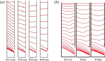
Figure 11. Profiles of the top surface of granular materials for various
 $W$
at constant time steps: (a) experiments with
$W$
at constant time steps: (a) experiments with
 $D=25$
mm,
$D=25$
mm,
 $d=190~\unicode[STIX]{x03BC}\text{m}$
, time interval
$d=190~\unicode[STIX]{x03BC}\text{m}$
, time interval
 $\unicode[STIX]{x0394}t_{e}=0.5$
s, (b) continuum simulation with
$\unicode[STIX]{x0394}t_{e}=0.5$
s, (b) continuum simulation with
 $D=56.25d$
and time interval
$D=56.25d$
and time interval
 $\unicode[STIX]{x0394}t_{s}/\sqrt{d/g}=9.5$
.
$\unicode[STIX]{x0394}t_{s}/\sqrt{d/g}=9.5$
.
Finally figure 11 shows the time evolution of the top surface of granular material for various silo widths for (a) the experiment and (b) the continuum simulation. From experiments we can see that the surface of particles begins to tilt in the early stage for a small width
 $W$
, whereas it remains constant till the last stage for the largest
$W$
, whereas it remains constant till the last stage for the largest
 $W$
. The tilted interface exhibits a slope starting from the wall opposite to the outlet and reaches a flattened surface, or sometimes even a small bump, on the wall containing the outlet. The slope of the interface is higher than the angle of repose for
$W$
. The tilted interface exhibits a slope starting from the wall opposite to the outlet and reaches a flattened surface, or sometimes even a small bump, on the wall containing the outlet. The slope of the interface is higher than the angle of repose for
 $W=3.5$
mm, and smaller than the angle of repose for
$W=3.5$
mm, and smaller than the angle of repose for
 $W=10$
mm. In continuum simulations, we explored a smaller range of
$W=10$
mm. In continuum simulations, we explored a smaller range of
 $W$
, the smallest
$W$
, the smallest
 $W$
case
$W$
case
 $W=13.5d$
, is comparable to the case
$W=13.5d$
, is comparable to the case
 $W=20$
mm in the experiments, but we clearly recover the same trend: the larger the thickness
$W=20$
mm in the experiments, but we clearly recover the same trend: the larger the thickness
 $W$
, the longer the interface remains symmetrical. Note also that the no-slip conditions imposed at the wall are not exactly the same as in the experiments, where a sliding velocity is observed. Nevertheless, the same qualitative profiles are obtained. This behaviour is consistent with the previous observation: for large
$W$
, the longer the interface remains symmetrical. Note also that the no-slip conditions imposed at the wall are not exactly the same as in the experiments, where a sliding velocity is observed. Nevertheless, the same qualitative profiles are obtained. This behaviour is consistent with the previous observation: for large
 $W$
, the flow far from the outlet is symmetrical. For small
$W$
, the flow far from the outlet is symmetrical. For small
 $W$
, the lateral friction breaks this symmetry and localises the flow on the side of the outlet, which inclines the surface in this direction.
$W$
, the lateral friction breaks this symmetry and localises the flow on the side of the outlet, which inclines the surface in this direction.
3.4 Experimental results in the cylindrical silo
The previous results were given for a simplified geometry, with a rectangular silo and an outlet which spans the width of the silo. Experimentally we also performed measurements of the flow rate for a cylindrical silo, with an outlet located at its side as schematised in figure 1(b). This situation generates a flow in a fully 3-D geometry, and is of practical interest. To characterise the different roles played by the length
 $D$
and the width
$D$
and the width
 $W$
of the outlet, we have plotted in figure 12 the dimensionless mass flow rate
$W$
of the outlet, we have plotted in figure 12 the dimensionless mass flow rate
 $Q/(\unicode[STIX]{x1D70C}\unicode[STIX]{x1D719}_{b}\sqrt{gW^{5}})$
as a function of the aperture aspect ratio
$Q/(\unicode[STIX]{x1D70C}\unicode[STIX]{x1D719}_{b}\sqrt{gW^{5}})$
as a function of the aperture aspect ratio
 $D/W$
, as done in the rectangular configuration.
$D/W$
, as done in the rectangular configuration.

Figure 12. Experimental results in the cylindrical silo: dimensionless mass flow rate
 $Q/(\unicode[STIX]{x1D70C}\unicode[STIX]{x1D719}_{b}\sqrt{gW^{5}})$
as a function of the aperture aspect ratio
$Q/(\unicode[STIX]{x1D70C}\unicode[STIX]{x1D719}_{b}\sqrt{gW^{5}})$
as a function of the aperture aspect ratio
 $D/W$
. The dashed line represents equation (3.2) with
$D/W$
. The dashed line represents equation (3.2) with
 $c_{D}=0.49$
, and the dashed-dotted line represents equation (3.3) with
$c_{D}=0.49$
, and the dashed-dotted line represents equation (3.3) with
 $c_{W}=0.46$
.
$c_{W}=0.46$
.
As suggested by the
 $\unicode[STIX]{x1D6F1}$
theorem in § 3.1 the data superimpose in this representation. Moreover, we observe the same behaviours as in rectangular silos. For large
$\unicode[STIX]{x1D6F1}$
theorem in § 3.1 the data superimpose in this representation. Moreover, we observe the same behaviours as in rectangular silos. For large
 $W$
, the flow rate follows the Hagen–Beverloo relation ((3.2), dashed line in the figure) and for small
$W$
, the flow rate follows the Hagen–Beverloo relation ((3.2), dashed line in the figure) and for small
 $W$
, the flow rate follows (3.3) (dashed-dotted line in the figure) suggesting that the flow is dominated by the lateral friction. Over the whole range, the data are well correlated by (3.4) (solid line in the figure) with
$W$
, the flow rate follows (3.3) (dashed-dotted line in the figure) suggesting that the flow is dominated by the lateral friction. Over the whole range, the data are well correlated by (3.4) (solid line in the figure) with
 $c_{D}=0.49$
and
$c_{D}=0.49$
and
 $c_{W}=0.46$
. The fitting parameter
$c_{W}=0.46$
. The fitting parameter
 $c_{w}$
is found to be slightly smaller than that in the rectangular silo. This suggests that the dissipation is higher in the cylinder, and more specifically in the regime controlled by the lateral friction where we can assume that the friction with a smooth lateral wall is smaller than that with an erodible granular media. Consequently, the transition between the two regimes occurs for a smaller aperture aspect ratio
$c_{w}$
is found to be slightly smaller than that in the rectangular silo. This suggests that the dissipation is higher in the cylinder, and more specifically in the regime controlled by the lateral friction where we can assume that the friction with a smooth lateral wall is smaller than that with an erodible granular media. Consequently, the transition between the two regimes occurs for a smaller aperture aspect ratio
 ${\mathcal{A}}_{c}\approx 1$
.
${\mathcal{A}}_{c}\approx 1$
.
3.5 Dependency of the flow rate on the particle diameter
The previous results are shown for a given small particle diameter
 $d=190~\unicode[STIX]{x03BC}\text{m}$
. In this section we focus on the influence of the particle diameter. We have shown that the flow rate of discharge of a silo with a lateral outlet depends on the aperture aspect ratio
$d=190~\unicode[STIX]{x03BC}\text{m}$
. In this section we focus on the influence of the particle diameter. We have shown that the flow rate of discharge of a silo with a lateral outlet depends on the aperture aspect ratio
 ${\mathcal{A}}=D/W$
, and exhibits two regimes of flow described by (3.2) for small
${\mathcal{A}}=D/W$
, and exhibits two regimes of flow described by (3.2) for small
 ${\mathcal{A}}$
and by (3.3) for large
${\mathcal{A}}$
and by (3.3) for large
 ${\mathcal{A}}$
. When the particle diameter is varied, these scaling relations seem to remain valid, as can been seen in figure 4(a,b) where the flow rate is plotted versus
${\mathcal{A}}$
. When the particle diameter is varied, these scaling relations seem to remain valid, as can been seen in figure 4(a,b) where the flow rate is plotted versus
 $D$
for two particle diameters,
$D$
for two particle diameters,
 $d=190~\unicode[STIX]{x03BC}\text{m}$
and
$d=190~\unicode[STIX]{x03BC}\text{m}$
and
 $d=1129~\unicode[STIX]{x03BC}\text{m}$
, in the two regimes. In each regime the same scaling is found for the two grain sizes, however we observe a shift of these relations towards smaller flow rates when the particle diameter increases. This behaviour can be seen in figure 13(a,c) where the dimensionless flow rate
$d=1129~\unicode[STIX]{x03BC}\text{m}$
, in the two regimes. In each regime the same scaling is found for the two grain sizes, however we observe a shift of these relations towards smaller flow rates when the particle diameter increases. This behaviour can be seen in figure 13(a,c) where the dimensionless flow rate
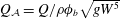 $Q_{{\mathcal{A}}}=Q/\unicode[STIX]{x1D70C}\unicode[STIX]{x1D719}_{b}\sqrt{gW^{5}}$
is plotted as a function of
$Q_{{\mathcal{A}}}=Q/\unicode[STIX]{x1D70C}\unicode[STIX]{x1D719}_{b}\sqrt{gW^{5}}$
is plotted as a function of
 $D/W$
for both the rectangular silos and the cylindrical silo for all the batch of particles we used. The two regimes are recovered whatever the particle diameter, see the dashed line and the dashed-dotted line. However there is a significant scattering of the data above the relation fitted for the smallest particle size
$D/W$
for both the rectangular silos and the cylindrical silo for all the batch of particles we used. The two regimes are recovered whatever the particle diameter, see the dashed line and the dashed-dotted line. However there is a significant scattering of the data above the relation fitted for the smallest particle size
 $d=190~\unicode[STIX]{x03BC}\text{m}$
.
$d=190~\unicode[STIX]{x03BC}\text{m}$
.

Figure 13. Mass flow rate
 $Q$
as a function of
$Q$
as a function of
 $D/W$
for various
$D/W$
for various
 $d$
for (a,c) rectangular silos and (b,d) cylindrical silos, normalised in (a,b) by
$d$
for (a,c) rectangular silos and (b,d) cylindrical silos, normalised in (a,b) by
 $(\unicode[STIX]{x1D70C}\unicode[STIX]{x1D719}_{b}\sqrt{gW^{5}})$
and in (c,d) by
$(\unicode[STIX]{x1D70C}\unicode[STIX]{x1D719}_{b}\sqrt{gW^{5}})$
and in (c,d) by
 $\unicode[STIX]{x1D70C}\unicode[STIX]{x1D719}_{b}\sqrt{gW^{5}}G_{D}(D/d)G_{W}(W/d)$
(see (3.12)) with the fitting parameters
$\unicode[STIX]{x1D70C}\unicode[STIX]{x1D719}_{b}\sqrt{gW^{5}}G_{D}(D/d)G_{W}(W/d)$
(see (3.12)) with the fitting parameters
 $\unicode[STIX]{x1D6FD}_{D}=\unicode[STIX]{x1D6FD}_{W}=0.1$
,
$\unicode[STIX]{x1D6FD}_{D}=\unicode[STIX]{x1D6FD}_{W}=0.1$
,
 $\unicode[STIX]{x1D6FC}_{D}=1$
and
$\unicode[STIX]{x1D6FC}_{D}=1$
and
 $\unicode[STIX]{x1D6FC}_{W}=0.46$
(see appendix A). The dashed and dashed-dotted lines are the same as in figures 5 and 12.
$\unicode[STIX]{x1D6FC}_{W}=0.46$
(see appendix A). The dashed and dashed-dotted lines are the same as in figures 5 and 12.
To model the dependency of the flow rate on the particle diameter, we follow the work of Janda et al. (Reference Janda, Zuriguel and Maza2012). In this framework we suppose that the particle size has to be accounted for through the number of beads in the aperture via a geometrical function, significant when this number is small. We take the two dimensions of the aperture into account and thus we suppose that the flow rate depends on two geometrical functions based on the number of beads in the aperture length
 $D/d$
and in the aperture width
$D/d$
and in the aperture width
 $W/d$
. The details of this approach and its validation using a 2-D discrete numerical simulation are given in the appendix. This yields the following expression for the flow rate:
$W/d$
. The details of this approach and its validation using a 2-D discrete numerical simulation are given in the appendix. This yields the following expression for the flow rate:
 $$\begin{eqnarray}Q=C_{l}^{\prime }\unicode[STIX]{x1D70C}\unicode[STIX]{x1D719}_{b}G_{D}\left(\frac{D}{d}\right)G_{W}\left(\frac{W}{d}\right)F\left(\frac{D}{W}\right)WD\sqrt{gD},\end{eqnarray}$$
with
 $G_{D}(D/d)=[1-\unicode[STIX]{x1D6FC}_{D}\text{e}^{-\unicode[STIX]{x1D6FD}_{D}(D/d)}]$
,
$G_{D}(D/d)=[1-\unicode[STIX]{x1D6FC}_{D}\text{e}^{-\unicode[STIX]{x1D6FD}_{D}(D/d)}]$
,
 $G_{W}(W/d)=[1-\unicode[STIX]{x1D6FC}_{W}\text{e}^{-\unicode[STIX]{x1D6FD}_{W}(W/d)}]$
and
$G_{W}(W/d)=[1-\unicode[STIX]{x1D6FC}_{W}\text{e}^{-\unicode[STIX]{x1D6FD}_{W}(W/d)}]$
and
 $F(D/W)=\sqrt{1/[1+\unicode[STIX]{x1D6FE}_{2}D/W]}$
.
$F(D/W)=\sqrt{1/[1+\unicode[STIX]{x1D6FE}_{2}D/W]}$
.
Figure 13 shows the normalised flow rate using the geometrical functions,
 $Q/[\unicode[STIX]{x1D70C}\unicode[STIX]{x1D719}_{b}G_{D}(D/d)G_{W}(W/d)\sqrt{gW^{5}}]$
, as a function of the aperture aspect ratio
$Q/[\unicode[STIX]{x1D70C}\unicode[STIX]{x1D719}_{b}G_{D}(D/d)G_{W}(W/d)\sqrt{gW^{5}}]$
, as a function of the aperture aspect ratio
 $D/W$
for the whole range of particle diameters for (c) rectangular silos and (d) cylindrical silos. In this representation the data collapse and can be well adjusted by the same asymptotic relations in two regimes as in figures 5 and 12.
$D/W$
for the whole range of particle diameters for (c) rectangular silos and (d) cylindrical silos. In this representation the data collapse and can be well adjusted by the same asymptotic relations in two regimes as in figures 5 and 12.
We propose additional analysis in the appendix. The 2-D discrete numerical simulation shows that the velocity at the outlet may follow the same geometrical relation than the volume fraction. As the continuum simulation described correctly most of the observations on the discharge of a silo with a lateral aperture for a given particle diameter we wonder if the continuum simulation is able to recover partially the dependency on the particle size of the flow rate. Indeed, the
 $\unicode[STIX]{x1D707}(I)$
rheology contains the information on the particle diameter in the definition of the inertial number
$\unicode[STIX]{x1D707}(I)$
rheology contains the information on the particle diameter in the definition of the inertial number
 $I=d\sqrt{2}D_{2}/(\sqrt{p/\unicode[STIX]{x1D70C}})$
. Even though a dependency on the particle diameter is observed in the 2-D case, the profiles present a larger asymmetry than the one predicted by the 2-D discrete simulations. This can be due to the fact that the volume fraction has been assumed to be uniform, whereas the complete
$I=d\sqrt{2}D_{2}/(\sqrt{p/\unicode[STIX]{x1D70C}})$
. Even though a dependency on the particle diameter is observed in the 2-D case, the profiles present a larger asymmetry than the one predicted by the 2-D discrete simulations. This can be due to the fact that the volume fraction has been assumed to be uniform, whereas the complete
 $\unicode[STIX]{x1D707}(I)$
-rheology, that includes a
$\unicode[STIX]{x1D707}(I)$
-rheology, that includes a
 $\unicode[STIX]{x1D719}(I)$
relation, would predict a dilation of the granular medium when it is sheared.
$\unicode[STIX]{x1D719}(I)$
relation, would predict a dilation of the granular medium when it is sheared.
4 Conclusion and perspectives
Using experiments, 2-D discrete simulations and continuum simulations we have studied the discharge of a silo with a lateral orifice. Experimentally we have observed two regimes of flow, either in a rectangular silo with an orifice spanning the thickness
 $W$
of the silo or in a cylindrical silo. The first regime, observed for small aperture aspect ratios
$W$
of the silo or in a cylindrical silo. The first regime, observed for small aperture aspect ratios
 ${\mathcal{A}}=D/W$
, corresponds to the well-known Hagen–Beverloo regime with a flow rate
${\mathcal{A}}=D/W$
, corresponds to the well-known Hagen–Beverloo regime with a flow rate
 $Q\propto WD^{3/2}$
. The second regime, observed for large aperture aspect ratios
$Q\propto WD^{3/2}$
. The second regime, observed for large aperture aspect ratios
 ${\mathcal{A}}>{\mathcal{A}}_{c}$
, follows
${\mathcal{A}}>{\mathcal{A}}_{c}$
, follows
 $Q\propto W^{3/2}D$
. We have proposed an empirical relation which predicts the flow rate depending on the aperture dimensions and which recovers both regimes. The continuum simulation, using the frictional
$Q\propto W^{3/2}D$
. We have proposed an empirical relation which predicts the flow rate depending on the aperture dimensions and which recovers both regimes. The continuum simulation, using the frictional
 $\unicode[STIX]{x1D707}(I)$
rheology and solved in two dimensions with an additional force to take into account the wall friction in a Hele-Shaw spirit, is found to describe qualitatively these two regimes and most of the internal details of the flow field observed experimentally in the rectangular silo, notably the fact that the velocity field is aligned with gravity when lateral wall friction is large. The dependency on the silo width suggests that the large
$\unicode[STIX]{x1D707}(I)$
rheology and solved in two dimensions with an additional force to take into account the wall friction in a Hele-Shaw spirit, is found to describe qualitatively these two regimes and most of the internal details of the flow field observed experimentally in the rectangular silo, notably the fact that the velocity field is aligned with gravity when lateral wall friction is large. The dependency on the silo width suggests that the large
 ${\mathcal{A}}$
regime is dominated by the lateral friction, and it seems reasonable to think that the small
${\mathcal{A}}$
regime is dominated by the lateral friction, and it seems reasonable to think that the small
 ${\mathcal{A}}$
regime is controlled by the internal friction.
${\mathcal{A}}$
regime is controlled by the internal friction.
We have found that the particle diameter matters only when the number of beads through the smallest orifice dimension is sufficiently small. The flow rate dependency on this parameter can be reasonably described using two geometrical functions
 $G_{\ell }(\ell /d)=1-\unicode[STIX]{x1D6FC}\text{e}^{-\unicode[STIX]{x1D6FD}\ell /d}$
based respectively on
$G_{\ell }(\ell /d)=1-\unicode[STIX]{x1D6FC}\text{e}^{-\unicode[STIX]{x1D6FD}\ell /d}$
based respectively on
 $W$
and on
$W$
and on
 $D$
. A large part of this behaviour is well reproduced using 2-D discrete simulations. Interestingly a dependency on the particle diameter is also observed in the 2-D continuum simulation but it predicts different velocity profiles which can be due to the fact that in the continuum simulation the volume fraction does not vary.
$D$
. A large part of this behaviour is well reproduced using 2-D discrete simulations. Interestingly a dependency on the particle diameter is also observed in the 2-D continuum simulation but it predicts different velocity profiles which can be due to the fact that in the continuum simulation the volume fraction does not vary.
In future work these promising observations need to be confirmed by conducting systematic 3-D simulations. Preliminary 3-D continuum simulation results indicate that the Hagen–Beverloo relation is obtained for a silo with bottom aperture. Extra developments have to be done to include realistic boundary conditions to represent particle–wall friction as well as the volume fraction variation
 $\unicode[STIX]{x1D719}(I)$
.
$\unicode[STIX]{x1D719}(I)$
.
Acknowledgements
We would like to thank P. Cervetti, S. Noel and F. Ratouchniak for technical assistance. This work has been carried out in the framework of the Labex MEC (ANR-10-LABX-0092) and of the A*MIDEX project (ANR-11-IDEX-0001-02), funded by the ‘Investissements d’Avenir’ French Government program managed by the French National Research Agency (ANR).
Supplementary material
Supplementary material is available at https://doi.org/10.1017/jfm.2017.543.
Appendix A. Additional analysis
In this section we focus on the influence of the particle diameter. We first present an analysis of the experimental results based on the work of Janda et al. (Reference Janda, Zuriguel and Maza2012). We then discuss the role of the particle diameter on the flow close to the outlet using 2-D contact dynamics simulations. Finally, we compare these results to the continuum numerical simulations.
A.1 Experimental results and discussion
To take the dependency on the particle diameter into account, as observed in figure 13(a,b), we suppose that the observations made experimentally by Janda et al. (Reference Janda, Zuriguel and Maza2012), and numerically by Zhou et al. (Reference Zhou, Ruyer and Aussillous2015) for a two-dimensional silo with an orifice placed at the bottom of the silo remain valid in our geometry. We make the following assumptions:
(i) We suppose that the horizontal velocity profile together with the density profile at the outlet are self-similar when varying the length of the hole
 $R=D/2$
. The flow rate is then given by
$R=D/2$
. The flow rate is then given by
 $$\begin{eqnarray}Q=\unicode[STIX]{x1D70C}W\iint _{-R}^{R}\unicode[STIX]{x1D719}(y)u(y)\,\text{d}y=c\unicode[STIX]{x1D70C}WD\bar{\unicode[STIX]{x1D719}}\bar{u},\end{eqnarray}$$
where
 $c$
is a constant of integration and
$c$
is a constant of integration and
 $\bar{\unicode[STIX]{x1D719}}$
and
$\bar{\unicode[STIX]{x1D719}}$
and
 $\bar{u}$
represent the mean density and the mean horizontal velocity at the outlet respectively. The flow rate is then determined by these two quantities.
$\bar{u}$
represent the mean density and the mean horizontal velocity at the outlet respectively. The flow rate is then determined by these two quantities.
(ii) Following (3.5), the mean horizontal velocity tends asymptotically as
 $d$
decreases towards
$d$
decreases towards
 $$\begin{eqnarray}\displaystyle \unicode[STIX]{x1D709}_{v}\displaystyle \sqrt{gD}\sqrt{\displaystyle \frac{1}{1+\unicode[STIX]{x1D6FE}_{2}D/W}}=\unicode[STIX]{x1D709}_{v}\sqrt{gD}F(D/W), & & \displaystyle\end{eqnarray}$$
where
 $F(D/W)=\sqrt{1/[1+\unicode[STIX]{x1D6FE}_{2}D/W]}$
, which corresponds to the value for infinitely small particles.
$F(D/W)=\sqrt{1/[1+\unicode[STIX]{x1D6FE}_{2}D/W]}$
, which corresponds to the value for infinitely small particles.
(iii) The granular medium tends to dilate at the outlet to maintain the flow. However for a large number of beads in the aperture, we suppose that it tends towards a fraction of the bulk density asymptotically,
 $\unicode[STIX]{x1D709}_{\unicode[STIX]{x1D719}}\unicode[STIX]{x1D719}_{b}$
, with
$\unicode[STIX]{x1D709}_{\unicode[STIX]{x1D719}}\unicode[STIX]{x1D719}_{b}$
, with
 $\unicode[STIX]{x1D709}_{\unicode[STIX]{x1D719}}$
a constant.
$\unicode[STIX]{x1D709}_{\unicode[STIX]{x1D719}}$
a constant.
(iv) We suppose that both the mean density and the mean velocity depend on the number of beads in the aperture via a geometrical function. To take the two dimensions of the aperture into account, we suppose that the flow rate depends on two geometrical functions based on the number of beads in the aperture length
 $D/d$
, and in the aperture width
$D/d$
, and in the aperture width
 $W/d$
. We assume that this geometrical function can be fitted by an exponential saturation
$W/d$
. We assume that this geometrical function can be fitted by an exponential saturation
 $$\begin{eqnarray}Q=C_{l}^{\prime }\unicode[STIX]{x1D70C}\unicode[STIX]{x1D719}_{b}G_{D}\left(\frac{D}{d}\right)G_{W}\left(\frac{W}{d}\right)F\left(\frac{D}{W}\right)WD\sqrt{gD},\end{eqnarray}$$
with
 $G_{D}(D/d)=[1-\unicode[STIX]{x1D6FC}_{D}\text{e}^{-\unicode[STIX]{x1D6FD}_{D}(D/d)}]$
and
$G_{D}(D/d)=[1-\unicode[STIX]{x1D6FC}_{D}\text{e}^{-\unicode[STIX]{x1D6FD}_{D}(D/d)}]$
and
 $G_{W}(W/d)=[1-\unicode[STIX]{x1D6FC}_{W}\text{e}^{-\unicode[STIX]{x1D6FD}_{W}(W/d)}]$
.
$G_{W}(W/d)=[1-\unicode[STIX]{x1D6FC}_{W}\text{e}^{-\unicode[STIX]{x1D6FD}_{W}(W/d)}]$
.

Figure 14. Experimental results obtained with rectangular silos: dimensionless flow rate
 $Q/(\unicode[STIX]{x1D70C}\unicode[STIX]{x1D719}_{b}WDF(D/W)\sqrt{gD})$
versus (a,b)
$Q/(\unicode[STIX]{x1D70C}\unicode[STIX]{x1D719}_{b}WDF(D/W)\sqrt{gD})$
versus (a,b)
 $D/d$
and (c,d)
$D/d$
and (c,d)
 $W/d$
. Selected experimental runs: (a,c) all the runs, (b)
$W/d$
. Selected experimental runs: (a,c) all the runs, (b)
 $D<1.8W$
and
$D<1.8W$
and
 $W>10d$
, (d)
$W>10d$
, (d)
 $D>2.2W$
and
$D>2.2W$
and
 $D>20d$
. The full lines represent the geometrical functions
$D>20d$
. The full lines represent the geometrical functions
 $G_{D}(D/d)=[1-\unicode[STIX]{x1D6FC}_{D}\text{e}^{-\unicode[STIX]{x1D6FD}_{D}(D/d)}]$
and
$G_{D}(D/d)=[1-\unicode[STIX]{x1D6FC}_{D}\text{e}^{-\unicode[STIX]{x1D6FD}_{D}(D/d)}]$
and
 $G_{W}(W/d)=[1-\unicode[STIX]{x1D6FC}_{W}\text{e}^{-\unicode[STIX]{x1D6FD}_{W}(W/d)}]$
with
$G_{W}(W/d)=[1-\unicode[STIX]{x1D6FC}_{W}\text{e}^{-\unicode[STIX]{x1D6FD}_{W}(W/d)}]$
with
 $\unicode[STIX]{x1D6FC}_{D}=1$
,
$\unicode[STIX]{x1D6FC}_{D}=1$
,
 $\unicode[STIX]{x1D6FD}_{D}=0.1$
,
$\unicode[STIX]{x1D6FD}_{D}=0.1$
,
 $\unicode[STIX]{x1D6FC}_{W}=0.46$
and
$\unicode[STIX]{x1D6FC}_{W}=0.46$
and
 $\unicode[STIX]{x1D6FD}_{W}=0.1$
respectively.
$\unicode[STIX]{x1D6FD}_{W}=0.1$
respectively.
To test these hypotheses, we isolated each geometrical function by plotting the dimensionless flow rate
 $Q/(\unicode[STIX]{x1D70C}\unicode[STIX]{x1D719}_{b}WDF(D/W)\sqrt{gD})$
as a function of the number of beads in the typical length
$Q/(\unicode[STIX]{x1D70C}\unicode[STIX]{x1D719}_{b}WDF(D/W)\sqrt{gD})$
as a function of the number of beads in the typical length
 $\ell /d$
for the two regimes (i)
$\ell /d$
for the two regimes (i)
 $\ell =D$
and (ii)
$\ell =D$
and (ii)
 $\ell =W$
. In figure 14(a,c) all the data for the rectangular silo are plotted and no clear trend can be observed. However, when considering each regime separately, as done in figure 14(b,d), i.e. by selecting the experiments corresponding to the first regime
$\ell =W$
. In figure 14(a,c) all the data for the rectangular silo are plotted and no clear trend can be observed. However, when considering each regime separately, as done in figure 14(b,d), i.e. by selecting the experiments corresponding to the first regime
 $\ell =D$
(and the second regime
$\ell =D$
(and the second regime
 $\ell =W$
), taking
$\ell =W$
), taking
 $D<1.8W$
(respectively
$D<1.8W$
(respectively
 $D>2.2W$
), and considering a large number of beads in the second direction of the orifice
$D>2.2W$
), and considering a large number of beads in the second direction of the orifice
 $W>10d$
(respectively
$W>10d$
(respectively
 $D>20d$
), the remaining data superimpose and can be well adjusted by an exponential saturation with the fitting parameters
$D>20d$
), the remaining data superimpose and can be well adjusted by an exponential saturation with the fitting parameters
 $\unicode[STIX]{x1D6FC}_{D}=1$
,
$\unicode[STIX]{x1D6FC}_{D}=1$
,
 $\unicode[STIX]{x1D6FD}_{D}=0.1$
,
$\unicode[STIX]{x1D6FD}_{D}=0.1$
,
 $\unicode[STIX]{x1D6FC}_{W}=0.46$
and
$\unicode[STIX]{x1D6FC}_{W}=0.46$
and
 $\unicode[STIX]{x1D6FD}_{W}=0.1$
(see the black lines in the figures). These parameters are of the same order of magnitude as that of the literature for both geometrical functions. It is interesting to note that the same
$\unicode[STIX]{x1D6FD}_{W}=0.1$
(see the black lines in the figures). These parameters are of the same order of magnitude as that of the literature for both geometrical functions. It is interesting to note that the same
 $\unicode[STIX]{x1D6FD}$
is recovered in the two directions. The same procedure has been followed for the cylindrical silo. Again, we find that both geometrical functions can be well adjusted by an exponential saturation, with the fitting parameters
$\unicode[STIX]{x1D6FD}$
is recovered in the two directions. The same procedure has been followed for the cylindrical silo. Again, we find that both geometrical functions can be well adjusted by an exponential saturation, with the fitting parameters
 $\unicode[STIX]{x1D6FC}_{D}=0.59$
,
$\unicode[STIX]{x1D6FC}_{D}=0.59$
,
 $\unicode[STIX]{x1D6FD}_{D}=0.08$
,
$\unicode[STIX]{x1D6FD}_{D}=0.08$
,
 $\unicode[STIX]{x1D6FC}_{W}=0.61$
, and
$\unicode[STIX]{x1D6FC}_{W}=0.61$
, and
 $\unicode[STIX]{x1D6FD}_{W}=0.08$
, in agreement with the literature.
$\unicode[STIX]{x1D6FD}_{W}=0.08$
, in agreement with the literature.
As shown in figure 13(c,d) it seems that the geometrical functions built on the two dimensions of the aperture correctly describe the dependency of the flow rate on the particle diameter. To further test some of the assumptions, we performed a 2-D discrete simulation of the discharge flow of a silo from a lateral orifice that allows to study the effective velocity and volume fraction profiles.
A.2 Discrete simulations in two dimensions
Discrete particle simulations are described in § 2.2. In this two-dimensional configuration, following the same methodology as for the bottom orifice done experimentally by Janda et al. (Reference Janda, Zuriguel and Maza2012) and with a 2-D discrete simulation by Zhou et al. (Reference Zhou, Ruyer and Aussillous2015), we are able to test most of the hypotheses (i) to (iv) made in the previous section for the Hagen–Beverloo regime.

Figure 15. (a–f) Flow of particles of diameter of
 $d=2$
mm for different outlet diameters. Vertical profiles of (a) the volume fraction,
$d=2$
mm for different outlet diameters. Vertical profiles of (a) the volume fraction,
 $\unicode[STIX]{x1D719}$
, (b) the horizontal velocity,
$\unicode[STIX]{x1D719}$
, (b) the horizontal velocity,
 $u$
, and (c) the vertical velocity,
$u$
, and (c) the vertical velocity,
 $v$
, versus the vertical position,
$v$
, versus the vertical position,
 $y$
. Vertical profiles of (d) the volume fraction normalised by the mean volume fraction,
$y$
. Vertical profiles of (d) the volume fraction normalised by the mean volume fraction,
 $\bar{\unicode[STIX]{x1D719}}$
, (e) the horizontal velocity made dimensionless by the mean horizontal velocity,
$\bar{\unicode[STIX]{x1D719}}$
, (e) the horizontal velocity made dimensionless by the mean horizontal velocity,
 $\bar{u}$
, and (f) the vertical velocity made dimensionless by the mean vertical velocity,
$\bar{u}$
, and (f) the vertical velocity made dimensionless by the mean vertical velocity,
 $\bar{v}$
, versus the position normalised by the outlet radius (
$\bar{v}$
, versus the position normalised by the outlet radius (
 $R=D/2$
). The full lines represent in (d) equation (A 4) with
$R=D/2$
). The full lines represent in (d) equation (A 4) with
 $\unicode[STIX]{x1D708}_{\unicode[STIX]{x1D719}}=0.21$
and in (e) equation (A 5) with
$\unicode[STIX]{x1D708}_{\unicode[STIX]{x1D719}}=0.21$
and in (e) equation (A 5) with
 $\unicode[STIX]{x1D708}_{v}=0.38$
respectively.
$\unicode[STIX]{x1D708}_{v}=0.38$
respectively.
(i) We have first assumed that at the lateral outlet, the horizontal velocity profile together with the density profile are self-similar when varying the length of the hole
 $R=D/2$
. Figure 15(a–c) shows the vertical profile of the volume fraction,
$R=D/2$
. Figure 15(a–c) shows the vertical profile of the volume fraction,
 $\unicode[STIX]{x1D719}$
, of the horizontal velocity,
$\unicode[STIX]{x1D719}$
, of the horizontal velocity,
 $u$
, and of the vertical velocity,
$u$
, and of the vertical velocity,
 $v$
, for various aperture lengths,
$v$
, for various aperture lengths,
 $D$
, for a given particle diameter
$D$
, for a given particle diameter
 $d=2$
mm. The vertical axis,
$d=2$
mm. The vertical axis,
 $y$
, is oriented upward and its origin is located at the middle of the outlet. Similar to the case of an aperture placed at the bottom of the silo, the volume fraction profile is found to be self-similar when normalised by the mean volume fraction,
$y$
, is oriented upward and its origin is located at the middle of the outlet. Similar to the case of an aperture placed at the bottom of the silo, the volume fraction profile is found to be self-similar when normalised by the mean volume fraction,
 $\bar{\unicode[STIX]{x1D719}}$
as shown in figure 15(d). The self-similar profile is slightly dissymmetrical, the top of the profile exhibiting a slightly higher dilatancy at the edge than at the bottom. Nevertheless, it can be well fitted by
$\bar{\unicode[STIX]{x1D719}}$
as shown in figure 15(d). The self-similar profile is slightly dissymmetrical, the top of the profile exhibiting a slightly higher dilatancy at the edge than at the bottom. Nevertheless, it can be well fitted by
 $$\begin{eqnarray}\unicode[STIX]{x1D719}(y)=\bar{\unicode[STIX]{x1D719}}\unicode[STIX]{x1D6FE}(\unicode[STIX]{x1D708}_{\unicode[STIX]{x1D719}})\left[1-\left(\frac{y}{R}\right)^{2}\right]^{\unicode[STIX]{x1D708}_{\unicode[STIX]{x1D719}}},\end{eqnarray}$$
where
 $\unicode[STIX]{x1D6FE}(\unicode[STIX]{x1D708})=(2/\sqrt{\unicode[STIX]{x03C0}})\unicode[STIX]{x1D6E4}(\unicode[STIX]{x1D708}+3/2)/\unicode[STIX]{x1D6E4}(\unicode[STIX]{x1D708}+1)$
. The fitting parameter,
$\unicode[STIX]{x1D6FE}(\unicode[STIX]{x1D708})=(2/\sqrt{\unicode[STIX]{x03C0}})\unicode[STIX]{x1D6E4}(\unicode[STIX]{x1D708}+3/2)/\unicode[STIX]{x1D6E4}(\unicode[STIX]{x1D708}+1)$
. The fitting parameter,
 $\unicode[STIX]{x1D708}_{\unicode[STIX]{x1D719}}=0.21\pm 0.01$
, obtained using the least squares method, is similar to that obtained for a bottom aperture
$\unicode[STIX]{x1D708}_{\unicode[STIX]{x1D719}}=0.21\pm 0.01$
, obtained using the least squares method, is similar to that obtained for a bottom aperture
 $\unicode[STIX]{x1D708}_{\unicode[STIX]{x1D719}}=0.19\pm 0.01$
by Zhou et al. (Reference Zhou, Ruyer and Aussillous2015). In the same way, once normalised by the mean horizontal velocity,
$\unicode[STIX]{x1D708}_{\unicode[STIX]{x1D719}}=0.19\pm 0.01$
by Zhou et al. (Reference Zhou, Ruyer and Aussillous2015). In the same way, once normalised by the mean horizontal velocity,
 $\bar{u}$
, the horizontal velocity profile is found to be self-similar and well adjusted by
$\bar{u}$
, the horizontal velocity profile is found to be self-similar and well adjusted by
 $$\begin{eqnarray}u(y)=\bar{u}\unicode[STIX]{x1D6FE}(\unicode[STIX]{x1D708}_{v})\left[1-\left(\frac{y}{R}\right)^{2}\right]^{\unicode[STIX]{x1D708}_{v}},\end{eqnarray}$$
with the fitting parameter,
 $\unicode[STIX]{x1D708}_{v}=0.38\pm 0.01$
obtained using the least-squares method. This parameter is identical to that obtained for the vertical velocity by Zhou et al. (Reference Zhou, Ruyer and Aussillous2015) in the silo with a bottom aperture. Finally, the horizontal velocity profile is also found to be self-similar. The self-similar profile is clearly non-symmetric, exhibiting mainly a linear profile on the main part of outlet with a maximum close to the top where the velocity decreases toward the edge. The first hypothesis is hence fulfilled and the flow rate is given by
$\unicode[STIX]{x1D708}_{v}=0.38\pm 0.01$
obtained using the least-squares method. This parameter is identical to that obtained for the vertical velocity by Zhou et al. (Reference Zhou, Ruyer and Aussillous2015) in the silo with a bottom aperture. Finally, the horizontal velocity profile is also found to be self-similar. The self-similar profile is clearly non-symmetric, exhibiting mainly a linear profile on the main part of outlet with a maximum close to the top where the velocity decreases toward the edge. The first hypothesis is hence fulfilled and the flow rate is given by
 $Q=c\unicode[STIX]{x1D70C}D\bar{\unicode[STIX]{x1D719}}\bar{u}$
, where
$Q=c\unicode[STIX]{x1D70C}D\bar{\unicode[STIX]{x1D719}}\bar{u}$
, where
 $c$
is a constant.
$c$
is a constant.

Figure 16. (a) Mean volume fraction at the outlet,
 $\bar{\unicode[STIX]{x1D719}}$
, (b) mean horizontal velocity,
$\bar{\unicode[STIX]{x1D719}}$
, (b) mean horizontal velocity,
 $\bar{u}$
, and (c) mean vertical velocity,
$\bar{u}$
, and (c) mean vertical velocity,
 $\bar{v}$
, versus the diameter apertures
$\bar{v}$
, versus the diameter apertures
 $D$
, for two particle diameters. (d) Mean volume fraction at the outlet,
$D$
, for two particle diameters. (d) Mean volume fraction at the outlet,
 $\bar{\unicode[STIX]{x1D719}}$
, normalised by the bulk volume fraction,
$\bar{\unicode[STIX]{x1D719}}$
, normalised by the bulk volume fraction,
 $\unicode[STIX]{x1D719}_{b}$
, (e) mean horizontal velocity,
$\unicode[STIX]{x1D719}_{b}$
, (e) mean horizontal velocity,
 $\bar{u}$
, made dimensionless by
$\bar{u}$
, made dimensionless by
 $\sqrt{gd}$
and (f) mean vertical velocity,
$\sqrt{gd}$
and (f) mean vertical velocity,
 $\bar{v}$
, made dimensionless by
$\bar{v}$
, made dimensionless by
 $\sqrt{gd}$
, versus the number of beads in the apertures
$\sqrt{gd}$
, versus the number of beads in the apertures
 $D/d$
, for two particle diameters. The full line represent in (d) equation (A 6) with
$D/d$
, for two particle diameters. The full line represent in (d) equation (A 6) with
 $\unicode[STIX]{x1D709}_{\unicode[STIX]{x1D719}}=0.87$
,
$\unicode[STIX]{x1D709}_{\unicode[STIX]{x1D719}}=0.87$
,
 $\unicode[STIX]{x1D6FC}_{\unicode[STIX]{x1D719}}=0.44$
and
$\unicode[STIX]{x1D6FC}_{\unicode[STIX]{x1D719}}=0.44$
and
 $\unicode[STIX]{x1D6FD}=0.15$
, in (e) equation (A 7) with
$\unicode[STIX]{x1D6FD}=0.15$
, in (e) equation (A 7) with
 $\unicode[STIX]{x1D709}_{u}=1.2$
,
$\unicode[STIX]{x1D709}_{u}=1.2$
,
 $\unicode[STIX]{x1D6FC}_{u}=0.98$
and
$\unicode[STIX]{x1D6FC}_{u}=0.98$
and
 $\unicode[STIX]{x1D6FD}=0.15$
and in (f) equation (A 8) with
$\unicode[STIX]{x1D6FD}=0.15$
and in (f) equation (A 8) with
 $\unicode[STIX]{x1D709}_{v}=0.45$
,
$\unicode[STIX]{x1D709}_{v}=0.45$
,
 $\unicode[STIX]{x1D6FC}_{v}=0.78$
and
$\unicode[STIX]{x1D6FC}_{v}=0.78$
and
 $\unicode[STIX]{x1D6FD}=0.15$
, respectively.
$\unicode[STIX]{x1D6FD}=0.15$
, respectively.
To test the hypotheses (ii)–(iv), we plotted the mean volume fraction,
 $\bar{\unicode[STIX]{x1D719}}$
and the mean horizontal and vertical velocities,
$\bar{\unicode[STIX]{x1D719}}$
and the mean horizontal and vertical velocities,
 $\bar{u}$
and
$\bar{u}$
and
 $\bar{v}$
, as a function of the aperture length,
$\bar{v}$
, as a function of the aperture length,
 $D$
, for two particles diameters,
$D$
, for two particles diameters,
 $d=2$
mm (○) and
$d=2$
mm (○) and
 $d=6$
mm (▵), as seen in figure 16 (a–c). Clearly, all the variables depend on the particle diameters. In figure 16(d–f), the same variables are plotted, normalised by the assumed asymptotic behaviour, as a function of the number of beads in the aperture. The data collapse on single curves, as observed for the silo with a bottom aperture, which are well adjusted by an exponential saturation as expected,
$d=6$
mm (▵), as seen in figure 16 (a–c). Clearly, all the variables depend on the particle diameters. In figure 16(d–f), the same variables are plotted, normalised by the assumed asymptotic behaviour, as a function of the number of beads in the aperture. The data collapse on single curves, as observed for the silo with a bottom aperture, which are well adjusted by an exponential saturation as expected,
 $$\begin{eqnarray}\displaystyle & \displaystyle \bar{\unicode[STIX]{x1D719}}=\unicode[STIX]{x1D709}_{\unicode[STIX]{x1D719}}\unicode[STIX]{x1D719}_{b}\left[1-\unicode[STIX]{x1D6FC}_{\unicode[STIX]{x1D719}}\text{e}^{-\unicode[STIX]{x1D6FD}(D/d)}\right]=\unicode[STIX]{x1D709}_{\unicode[STIX]{x1D719}}\unicode[STIX]{x1D719}_{b}G_{\unicode[STIX]{x1D719}}\left(\frac{D}{d}\right), & \displaystyle\end{eqnarray}$$
 $$\begin{eqnarray}\displaystyle & \displaystyle \bar{u}=\unicode[STIX]{x1D709}_{u}\sqrt{gD}\left[1-\unicode[STIX]{x1D6FC}_{u}\text{e}^{-\unicode[STIX]{x1D6FD}(D/d)}\right]=\unicode[STIX]{x1D709}_{u}\sqrt{gD}G_{u}\left(\frac{D}{d}\right), & \displaystyle\end{eqnarray}$$
 $$\begin{eqnarray}\displaystyle & \displaystyle \bar{v}=\unicode[STIX]{x1D709}_{v}\sqrt{gD}\left[1-\unicode[STIX]{x1D6FC}_{v}\text{e}^{-\unicode[STIX]{x1D6FD}(D/d)}\right]=\unicode[STIX]{x1D709}_{v}\sqrt{gD}G_{v}\left(\frac{D}{d}\right), & \displaystyle\end{eqnarray}$$
with the fitting parameters
 $\unicode[STIX]{x1D6FD}=0.15$
,
$\unicode[STIX]{x1D6FD}=0.15$
,
 $\unicode[STIX]{x1D709}_{\unicode[STIX]{x1D719}}=0.87$
,
$\unicode[STIX]{x1D709}_{\unicode[STIX]{x1D719}}=0.87$
,
 $\unicode[STIX]{x1D6FC}_{\unicode[STIX]{x1D719}}=0.44$
,
$\unicode[STIX]{x1D6FC}_{\unicode[STIX]{x1D719}}=0.44$
,
 $\unicode[STIX]{x1D709}_{u}=1.2$
,
$\unicode[STIX]{x1D709}_{u}=1.2$
,
 $\unicode[STIX]{x1D6FC}_{u}=0.98$
,
$\unicode[STIX]{x1D6FC}_{u}=0.98$
,
 $\unicode[STIX]{x1D709}_{v}=0.45$
,
$\unicode[STIX]{x1D709}_{v}=0.45$
,
 $\unicode[STIX]{x1D6FC}_{v}=0.78$
, obtained using the least-squares method. Once again, these parameters closely match those obtained by Zhou et al. (Reference Zhou, Ruyer and Aussillous2015) for the bottom configuration. The same
$\unicode[STIX]{x1D6FC}_{v}=0.78$
, obtained using the least-squares method. Once again, these parameters closely match those obtained by Zhou et al. (Reference Zhou, Ruyer and Aussillous2015) for the bottom configuration. The same
 $\unicode[STIX]{x1D6FD}$
, fitted on the volume fraction, is found to correctly adjust the mean velocity variations. This suggests that the same phenomenon is involved in the variation at the outlet of the volume fraction and of the velocities with respect to the particle size. These equations also suggest that in the Hagen–Beverloo regime, the angle of inclination of the streamline at the outlet, defined as
$\unicode[STIX]{x1D6FD}$
, fitted on the volume fraction, is found to correctly adjust the mean velocity variations. This suggests that the same phenomenon is involved in the variation at the outlet of the volume fraction and of the velocities with respect to the particle size. These equations also suggest that in the Hagen–Beverloo regime, the angle of inclination of the streamline at the outlet, defined as
 $\tan (\unicode[STIX]{x1D703})=\bar{u}/\bar{v}$
has low dependency on the outlet size
$\tan (\unicode[STIX]{x1D703})=\bar{u}/\bar{v}$
has low dependency on the outlet size
 $D$
through a geometrical function
$D$
through a geometrical function
 $G_{u}/G_{v}$
. Finally the flow rate is given by
$G_{u}/G_{v}$
. Finally the flow rate is given by
 $$\begin{eqnarray}Q=C_{l}^{\prime }\unicode[STIX]{x1D70C}\unicode[STIX]{x1D719}_{b}\sqrt{gD}G_{\unicode[STIX]{x1D719}}\left(\frac{D}{d}\right)G_{u}\left(\frac{D}{d}\right)\approx C_{l}^{\prime }\unicode[STIX]{x1D70C}\unicode[STIX]{x1D719}_{b}\sqrt{gD}G\left(\frac{D}{d}\right),\end{eqnarray}$$
where
 $C_{l}^{\prime }=\unicode[STIX]{x1D709}_{\unicode[STIX]{x1D719}}\unicode[STIX]{x1D709}_{v}\unicode[STIX]{x1D6FE}(\unicode[STIX]{x1D708}_{v})\unicode[STIX]{x1D6FE}(\unicode[STIX]{x1D708}_{\unicode[STIX]{x1D719}})\int _{0}^{1}(1-t^{2})\,\text{d}t=1.08$
and
$C_{l}^{\prime }=\unicode[STIX]{x1D709}_{\unicode[STIX]{x1D719}}\unicode[STIX]{x1D709}_{v}\unicode[STIX]{x1D6FE}(\unicode[STIX]{x1D708}_{v})\unicode[STIX]{x1D6FE}(\unicode[STIX]{x1D708}_{\unicode[STIX]{x1D719}})\int _{0}^{1}(1-t^{2})\,\text{d}t=1.08$
and
 $G=[1-\unicode[STIX]{x1D6FC}\text{e}^{-\unicode[STIX]{x1D6FD}(D/d)}]$
with
$G=[1-\unicode[STIX]{x1D6FC}\text{e}^{-\unicode[STIX]{x1D6FD}(D/d)}]$
with
 $\unicode[STIX]{x1D6FC}=\unicode[STIX]{x1D6FC}_{\unicode[STIX]{x1D719}}+\unicode[STIX]{x1D6FC}_{u}$
. In the range of number of beads in the aperture (
$\unicode[STIX]{x1D6FC}=\unicode[STIX]{x1D6FC}_{\unicode[STIX]{x1D719}}+\unicode[STIX]{x1D6FC}_{u}$
. In the range of number of beads in the aperture (
 $D/d>6$
), the approximation of
$D/d>6$
), the approximation of
 $G\approx G_{u}G_{\unicode[STIX]{x1D719}}$
leads to less than
$G\approx G_{u}G_{\unicode[STIX]{x1D719}}$
leads to less than
 $5\,\%$
of error. This equation adjusts the data well with the fitting parameter
$5\,\%$
of error. This equation adjusts the data well with the fitting parameter
 $C_{l}^{\prime }=1.08$
, as seen in figure 17, and is similar to (A 3) considering
$C_{l}^{\prime }=1.08$
, as seen in figure 17, and is similar to (A 3) considering
 $W=\infty$
.
$W=\infty$
.

Figure 17. Flow rate made dimensionless by
 $\sqrt{gd^{3}}$
versus the number of beads in the aperture
$\sqrt{gd^{3}}$
versus the number of beads in the aperture
 $D/d$
for the 2-D case, (a) discrete simulation, (b) continuum simulation. The full lines represent equation (A 9) with (a)
$D/d$
for the 2-D case, (a) discrete simulation, (b) continuum simulation. The full lines represent equation (A 9) with (a)
 $C_{l}^{\prime }=1.08$
and (b)
$C_{l}^{\prime }=1.08$
and (b)
 $C_{l}^{\prime }=0.78$
.
$C_{l}^{\prime }=0.78$
.
Using 2-D discrete simulations we have shown that the dependence of the flow rate on the particle size can be modelled using a geometrical function which depends only on the number of beads in the aperture. This geometrical function is seen to influence both the volume fraction at the outlet, bigger particles leading to a dilation, and the velocity, bigger particles leading to slower flow. It would be interesting in future work to conduct 3-D discrete simulations to see if we recover the same geometrical function for the number of beads in the silo width, in the regime dominated by the lateral friction, as suggested by the experimental results.
A.3 Continuum simulation
We have seen in § 3 that the continuum simulation described correctly most of the observations on the discharge of a silo with a lateral aperture, for various
 $D$
and various
$D$
and various
 $W$
but for a given particle diameter. However the
$W$
but for a given particle diameter. However the
 $\unicode[STIX]{x1D707}(I)$
rheology contains the information on the particle diameter in the definition of the inertial number
$\unicode[STIX]{x1D707}(I)$
rheology contains the information on the particle diameter in the definition of the inertial number
 $I=d\sqrt{2}D_{2}/(\sqrt{p/\unicode[STIX]{x1D70C}})$
. In this section we wonder if the continuum simulation is able to recover partially the dependency on the particle size of the flow rate. Indeed, even if this simulation considers a constant volume fraction, the 2-D discrete simulations have shown that the velocity at the outlet may follow the same geometrical relation than the volume fraction.
$I=d\sqrt{2}D_{2}/(\sqrt{p/\unicode[STIX]{x1D70C}})$
. In this section we wonder if the continuum simulation is able to recover partially the dependency on the particle size of the flow rate. Indeed, even if this simulation considers a constant volume fraction, the 2-D discrete simulations have shown that the velocity at the outlet may follow the same geometrical relation than the volume fraction.
Figure 18 presents the vertical profile at the outlet of the horizontal velocity, the vertical velocity and the norm of the velocity, for a given particle diameter in the 2-D case. Interestingly, when normalised by the mean value, these profiles are again found to be self-similar. However, contrary to the discrete simulations, the horizontal velocity profile exhibits a strong asymmetry between the top and the bottom of the outlet. As a consequence, the adjustment by the (A 5) with the fitting parameter
 $\unicode[STIX]{x1D708}_{u}=0.31\pm 0.01$
obtained using least-squares method is not satisfactory. However the vertical velocity profile resembles the discrete simulation result. Interestingly, the profile of the norm of the velocity is found to remain symmetrical and is well adjusted by (A 5) with
$\unicode[STIX]{x1D708}_{u}=0.31\pm 0.01$
obtained using least-squares method is not satisfactory. However the vertical velocity profile resembles the discrete simulation result. Interestingly, the profile of the norm of the velocity is found to remain symmetrical and is well adjusted by (A 5) with
 $\unicode[STIX]{x1D708}_{v}=0.31$
.
$\unicode[STIX]{x1D708}_{v}=0.31$
.

Figure 18. Two-dimensional continuum simulation (a,d) horizontal velocity (b,e) vertical velocity and (c,f) norm of the velocity, (a–c) normalised by
 $\sqrt{gd}$
versus
$\sqrt{gd}$
versus
 $y/d$
and (d–f) normalised by the mean value versus
$y/d$
and (d–f) normalised by the mean value versus
 $y/R$
, the full lines in (d,f) represent equation (A 5) with
$y/R$
, the full lines in (d,f) represent equation (A 5) with
 $\unicode[STIX]{x1D708}_{v}=0.31$
.
$\unicode[STIX]{x1D708}_{v}=0.31$
.
Figure 19(a–c) shows the mean value of the horizontal and vertical velocities and of the norm of the velocity, normalised by
 $\sqrt{gL}$
versus the dimensionless outlet diameter
$\sqrt{gL}$
versus the dimensionless outlet diameter
 $D/d$
for two particles diameters
$D/d$
for two particles diameters
 $d=L/30$
and
$d=L/30$
and
 $d=L/90$
. Clearly these mean velocities depend on the outlet size
$d=L/90$
. Clearly these mean velocities depend on the outlet size
 $D$
, but also on the particle diameter
$D$
, but also on the particle diameter
 $d$
. Following the discrete simulation study we have plotted in figure 19(d–f) these velocities made dimensionless with
$d$
. Following the discrete simulation study we have plotted in figure 19(d–f) these velocities made dimensionless with
 $\sqrt{gD}$
versus
$\sqrt{gD}$
versus
 $D/d$
. The data corresponding to the mean horizontal velocity (respectively to the mean norm) are reasonably well adjusted by (A 7) with the fitting parameters
$D/d$
. The data corresponding to the mean horizontal velocity (respectively to the mean norm) are reasonably well adjusted by (A 7) with the fitting parameters
 $\unicode[STIX]{x1D6FD}=0.05$
,
$\unicode[STIX]{x1D6FD}=0.05$
,
 $\unicode[STIX]{x1D709}_{u}=0.78$
and
$\unicode[STIX]{x1D709}_{u}=0.78$
and
 $\unicode[STIX]{x1D6FC}_{u}=0.25$
(respectively
$\unicode[STIX]{x1D6FC}_{u}=0.25$
(respectively
 $\unicode[STIX]{x1D709}_{U}=1.06$
and
$\unicode[STIX]{x1D709}_{U}=1.06$
and
 $\unicode[STIX]{x1D6FC}_{U}=0.28$
). The value of
$\unicode[STIX]{x1D6FC}_{U}=0.28$
). The value of
 $\unicode[STIX]{x1D6FD}$
is sensibly lower than the value obtained experimentally or in the discrete simulation. However the same tendency than observed in the discrete simulation is recovered. This is not the case for the mean vertical velocity for which the data do not follow the asymptotic behaviour in
$\unicode[STIX]{x1D6FD}$
is sensibly lower than the value obtained experimentally or in the discrete simulation. However the same tendency than observed in the discrete simulation is recovered. This is not the case for the mean vertical velocity for which the data do not follow the asymptotic behaviour in
 $\sqrt{gD}$
. However this velocity is not involved in the flow rate and the (A 9) using the fitting parameters predicts well the flow rate, see the full line in figure 17(b).
$\sqrt{gD}$
. However this velocity is not involved in the flow rate and the (A 9) using the fitting parameters predicts well the flow rate, see the full line in figure 17(b).

Figure 19. Two-dimensional continuum simulation: (a,d) horizontal velocity, (b,e) vertical velocity and (c,f) norm of the velocity normalised in (a–c) by
 $\sqrt{gL}$
versus
$\sqrt{gL}$
versus
 $D/L$
and normalised in (d–f) by
$D/L$
and normalised in (d–f) by
 $\sqrt{gD}$
versus
$\sqrt{gD}$
versus
 $D/d$
for two particles diameters. The full lines in (d–f) represent equation (A 7) with the fitting parameters
$D/d$
for two particles diameters. The full lines in (d–f) represent equation (A 7) with the fitting parameters
 $\unicode[STIX]{x1D6FD}=0.05$
,
$\unicode[STIX]{x1D6FD}=0.05$
,
 $\unicode[STIX]{x1D709}_{u}=0.78$
,
$\unicode[STIX]{x1D709}_{u}=0.78$
,
 $\unicode[STIX]{x1D6FC}_{u}=0.25$
,
$\unicode[STIX]{x1D6FC}_{u}=0.25$
,
 $\unicode[STIX]{x1D709}_{v}=0.68$
,
$\unicode[STIX]{x1D709}_{v}=0.68$
,
 $\unicode[STIX]{x1D6FC}_{v}=0.31$
,
$\unicode[STIX]{x1D6FC}_{v}=0.31$
,
 $\unicode[STIX]{x1D709}_{U}=1.06$
and
$\unicode[STIX]{x1D709}_{U}=1.06$
and
 $\unicode[STIX]{x1D6FC}_{U}=0.28$
obtained using the least-squares method.
$\unicode[STIX]{x1D6FC}_{U}=0.28$
obtained using the least-squares method.
Finally we have done the same analysis in the pseudo-3-D continuum simulation, in the regime controlled by the side wall friction. Figure 20(a) presents the profile of the horizontal velocity at the outlet for various
 $D$
. In this regime, the profiles present the same asymmetric shape than in the Hagen–Beverloo profile, nevertheless the velocity does not seem to depend on
$D$
. In this regime, the profiles present the same asymmetric shape than in the Hagen–Beverloo profile, nevertheless the velocity does not seem to depend on
 $D$
anymore. Figure 20(b) shows the mean horizontal velocity, normalised by
$D$
anymore. Figure 20(b) shows the mean horizontal velocity, normalised by
 $\sqrt{gW}$
versus
$\sqrt{gW}$
versus
 $W/d$
for data corresponding to the second regime,
$W/d$
for data corresponding to the second regime,
 $D/W>3$
. Clearly we do not observe the geometrical function as suggested by the experimental results. This is not surprising as the flow is not solved throughout the silo width, thus the
$D/W>3$
. Clearly we do not observe the geometrical function as suggested by the experimental results. This is not surprising as the flow is not solved throughout the silo width, thus the
 $I$
number is not expected to play any role in this direction.
$I$
number is not expected to play any role in this direction.
To conclude this section, we found that a dependency on the particle diameter is observed in the 2-D continuum simulation, that the velocity profiles are self-similar when varying the outlet length, and that the mean horizontal velocity tends asymptotically towards
 $\sqrt{gD}$
, contrary to the mean vertical velocity. This behaviour is well described by a geometrical function given by (A 7). However the profiles present a larger asymmetry than the one predicted by the 2-D discrete simulations. This can be due to the fact that the volume fraction has been assumed to be uniform, whereas the complete
$\sqrt{gD}$
, contrary to the mean vertical velocity. This behaviour is well described by a geometrical function given by (A 7). However the profiles present a larger asymmetry than the one predicted by the 2-D discrete simulations. This can be due to the fact that the volume fraction has been assumed to be uniform, whereas the complete
 $\unicode[STIX]{x1D707}(I)$
-rheology, that includes a
$\unicode[STIX]{x1D707}(I)$
-rheology, that includes a
 $\unicode[STIX]{x1D719}(I)$
relation, would predict a dilation of a granular media when it is sheared. The dependency on the particle diameter for the regime controlled by the side walls is not correctly described by the pseudo-3-D continuum simulation which does not solve the flow in the silo width direction.
$\unicode[STIX]{x1D719}(I)$
relation, would predict a dilation of a granular media when it is sheared. The dependency on the particle diameter for the regime controlled by the side walls is not correctly described by the pseudo-3-D continuum simulation which does not solve the flow in the silo width direction.

Figure 20. Pseudo-3-D continuum simulation. (a) Horizontal velocity normalised by
 $\sqrt{gd}$
versus
$\sqrt{gd}$
versus
 $y/d$
at the outlet for different
$y/d$
at the outlet for different
 $D$
and
$D$
and
 $W=13.5d$
; (b) mean horizontal velocity normalised by
$W=13.5d$
; (b) mean horizontal velocity normalised by
 $\sqrt{gW}$
for
$\sqrt{gW}$
for
 $D/W>3$
.
$D/W>3$
.


