2.1. Design principle and shock-tube details

A sketch of the entire shock-tube facility is shown in figure 1, in which the scales do not exactly reflect the real ones. The main bodies of all the sections of the shock-tube facility are made of steel. To produce two successive shock waves, a driver section (I) together with two identical transparent acrylic devices (acrylic devices I and II), is added between the driver section (II) and the driven section of a standard shock tube. For the driver sections I and II, the acrylic devices I and II and the driven section, the inner cross-section is circular with a radius of 30 mm. Gases in the driver sections II and I (the driver section I and the driven section) are separated by a polyester membrane embedded in the acrylic device II (I). Note that in this work, the gases in all regions are air unless specifically defined. The distance between the polyester membrane embedded in the acrylic device II and the inner end wall of the driver section II and the distance between two polyester membranes are 1750 and 700 mm, respectively. The distance between the polyester membrane embedded in the acrylic device I and the right-hand end of the driven section is 1470 mm. To avoid confusion, the region between the polyester membrane embedded in the acrylic device II and the end wall of the driver section II, and the region between two polyester membranes are hereinafter referred to as the driver section II and the driver section I, respectively.

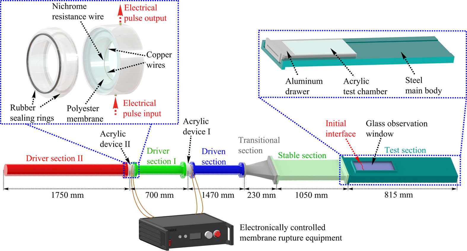
Figure 1. Sketch of the shock-tube facility for generating two successive shock waves.

To precisely control the initial Mach numbers of two shock waves, i.e. the initial pressures in two driver sections, and to achieve the synchronous generation of two shock waves, i.e. the synchronization of the rupture of membranes, an electronically controlled membrane rupture equipment (ECMRE) is adopted. The ECMRE is generally used to produce a high-voltage electrical pulse to heat the resistance wire in contact with the membrane, resulting in localized melting of the membrane, reducing its pressure-bearing capacity and thus achieving the rupture of the membrane. Compared with the traditional membrane rupture method, i.e. rupture the membrane directly through the pressure difference across it, an active rupture of the membrane can be realized by the ECMRE, and thus the timing of the membrane rupture and the pressures on both sides of the membrane when it ruptures can be precisely controlled. When the current through the resistance wire is high enough, the resistance wire will explode and the rupture of the membrane with a high quality can generally be achieved. If the blast wave generated by the explosion of the resistance wire is strong, it may introduce additional disturbances to the flow. The ECMRE adopted in the present work can produce two synchronous high-voltage electrical pulses, with output voltage up to 500 V and output current up to 2000 A. To illustrate the experimental set-up more clearly, an enlarged view of the acrylic device II is shown in figure 1. The polyester membrane is placed between the two parts of the acrylic device II and is held by the rubber sealing ring during the experiment. The thickness of the membrane depends on the preset pressure difference across it. Generally, to ensure the success and the repeatability of the experiment, it is desirable that the pressure-bearing capacity of the membrane is close to the preset pressure difference across it. A nichrome resistance wire with its ends connecting to the copper wires of very low resistance is in contact with the membrane. Before each experimental run, we first charge the energy-storage capacitor of the ECMRE to the required voltage. Since the resistances of the nichrome resistance wires attached to the polyester membranes are low (approximately 0.26 $\Omega$) and they are connected in parallel, the voltage selected in experiments is 250 V to avoid the damage to the ECMRE due to the excessive current. Then the ECMRE is triggered to produce two synchronous electrical pulses, causing the explosion of the nichrome resistance wires. When the polyester membranes rupture, two shock waves, two contact surfaces and two rarefaction waves are generated. These shock waves propagate from the driven section to the stable section with a rectangular cross-section of $140\,{\rm mm} \times 20\,{\rm mm}$ through a transitional section with a length of 230 mm. Note that in the transitional section where the cross-section changes from circular to rectangular, the cross-section area changes from 2827 to 2800 mm$^2$. The area change is negligible and the transition of the cross-section is smooth, which ensure that the intensities of the shock waves would not be significantly affected. The stable section with a length of 1050 mm is adopted to stabilize the shock waves before they enter the test section. In this work, the soap-film technique is adopted to create the initial single-mode interface. A single-mode soap-film interface has a minimum-surface feature (Luo, Wang & Si Reference Luo, Wang and Si2013) and its three-dimensionality is highly related to its height. For investigating a quasi-two-dimensional SSS-RMI phenomenon, the cross-section is changed from $140\,{\rm mm}\times 20\,{\rm mm}$ to $140\,{\rm mm}\times 6\,{\rm mm}$ at the junction of the stable section with the test section to weaken the three-dimensionality of the soap-film interface generated in experiments. Inevitably, the cross-section truncation will have some effects on the shock intensities and the flow. This will be discussed in Appendix A.

As shown in figure 1, the test section mainly consists of four parts: the steel main body; the glass observation window; the transparent acrylic test chamber; and the aluminium drawer. The length of the test section is 815 mm, which ensures that the rarefaction waves generated when the first shock wave exits the open end of the test section would not affect the development of the interface. The observation window made of K9 optical glass has a width of 95 mm and a length of 275 mm, and its left-hand side is 75 mm away from the junction of the stable section with the test section. The transparent acrylic test chamber is served as the interface formation device when performing experiments with the soap-film interfaces. For the soap-film technique, readers can find more details in our previous works (Liu et al. Reference Liu, Liang, Ding, Liu and Luo2018; Liang et al. Reference Liang, Zhai, Ding and Luo2019).

To investigate the SSS-RMI, there are three key objectives of designing the shock-tube facility. The first is the reliable and repeatable generation of two successive shock waves. The second is the controllable variations of the shock intensities and the time interval between two shock waves arriving at a given position, which are necessary to investigate the effects of different initial conditions on the flow. Intuitively, the shock intensities can be manipulated by changing the pressure ratios across the membranes, and the time interval can be regulated by varying the distance between the initial positions of two shock waves, the distance from the initial position of the first shock to the test section and the intensities of two shock waves. The third is the generation of a relatively ‘clean’ flow field, which means that the interface is accelerated by two shock waves but is not significantly affected by other waves. Note that although the flow just after the rupture of the membranes can be considered as a combination of two standard shock-tube flows, waves and contact surfaces would then interact with each other, making the flow field far complicated than that in a conventional shock tube. As a result, the flow in such a shock tube must be at least qualitatively well understood.

2.2. Shock-tube flow analysis

We first consider the one-dimensional (1-D) shock-tube flow. Figure 2 shows the distributions of flow regions before and after the membranes rupture. Gases in all sections are air. After the membranes rupture, as indicated in figure 2 at $t=t_1$, two shock waves (SW$_1$ and SW$_2$), two contact surfaces (CS$_1$ and CS$_2$) and two rarefaction waves (RW$_1$ and RW$_2$) are generated, and the flow can be divided into seven regions. In fact, the flow in this shock tube at $t=t_1$ can be considered as a combination of two standard shock-tube flows. Therefore, given the initial parameters, including the pressure ($p$) and the temperature ($T$) in the driven section (region 1), the driver section I (region 2) and the driver section II (region 3), the initial intensities of the two shock waves can be obtained by shock-tube theory (Glass & Hall Reference Glass and Hall1959; Owczarek Reference Owczarek1964; Han & Yin Reference Han and Yin1993)

(2.1)\begin{equation} \frac {p_h}{p_l} = \left[1+\frac{2\gamma_l}{\gamma_l+1}(M_{s}^2-1)\right] \left[1-\frac {\gamma_h-1}{\gamma_l+1} \frac {c_l}{c_h}\left(M_{s}-\frac {1}{M_{s}}\right)\right]^{{({-}2\gamma_h)}/{(\gamma_h-1)}}, \end{equation}

where subscript ‘$h$’ (‘$l$’) denotes the flow region with higher (lower) pressure, $M_s$ is the Mach number of the shock generated. Here $\gamma$ and $c$ are the specific heat ratio and sound speed, respectively. Once the shock Mach numbers are known, the flow parameters in regions 4 and 6 (behind the shock waves) can be calculated by normal shock relations ((B1)–(B5) in Appendix B). The flow Mach numbers ($M'$) in regions 5 and 7 (behind the rarefaction waves) can also be calculated by shock-tube theory

(2.2)\begin{equation} M'=\left[\frac{c_h}{c_l} \frac{(\gamma_l+1)M_s}{2(M_s^2-1)}-\frac{\gamma_h-1}{2}\right]^{{-}1}, \end{equation}

and other flow parameters such as pressure $p'$, density $\rho '$, temperature $T'$, speed of sound $c'$ and velocity $u'$ can be easily deduced by (B6)–(B10) in Appendix B. Superscript ‘$'$’ denotes the flow region between rarefaction waves and contact surface.

Figure 2. Distributions of flow regions before and after the rupture of membranes. Here SW refers to shock wave, CS or CR refers to contact surface or contact region and RW refers to rarefaction waves. Superscripts ‘$r$’ and ‘$t$’ denote reflected and transmitted, respectively. Here $t_0$ and $t_1$ are the moments before and shortly after the membranes rupture, respectively; $t_2$ is the moment after the shock SW$_2$ interacts with the rarefaction waves RW$_1$; $t_3$ is the moment after the shock SW$_2^{t}$ interacts with the contact surface CS$_1$, and after the rarefaction waves RW$_1^{t}$ interact with the contact surface CS$_2$, and after the rarefaction waves RW$_2$ reflect from the end wall. The shade of the colour generally indicates the magnitude of pressure.

However, as time proceeds, the flow in our new facility becomes far more complicated than that in the standard shock tube because there are many wave–wave and wave–contact surface interactions. We first assume that the driver section II is long enough, which allows the first three of four interactions considered below to occur before they are affected by the reflected rarefaction waves (RW$_2^{r}$) of RW$_2$ from the end wall.

(I) The interaction of the SW$_2$ with the RW$_1$ generates a transmitted shock (SW$_2^{t}$), transmitted rarefaction waves (RW$_1^{t}$) and a contact region (CR), as shown in figure 2 at $t=t_2$. The corresponding $x$–$t$ diagram is shown in figure 3(a). The intensity of the RW$_1^{t}$ is weaker than that of the RW$_1$, while the intensity of the SW$_2^{t}$ increases gradually during the interaction. As a result, a non-isentropic contact region CR, rather than a contact surface, is generated between the SW$_2^{t}$ and the RW$_1^{t}$. From region 2 to region 6, the variations of flow parameters satisfy the normal shock relations ((B1)–(B5) in Appendix B), and from region 6 to region 9, the variations of parameters satisfy the isentropic wave relations ((B11)–(B12) in Appendix B). From region 2 to region 5 and from region 5 to region 8, the variations of the flow parameters similarly satisfy the isentropic wave relations and the normal shock relations, respectively. In addition, the pressures and flow velocities at both sides of CR, i.e. regions 8 and 9, are the same. By combining these relations, the intensities of both the SW$_2^{t}$ and the RW$_1^{t}$ and the flow parameters in regions 8 and 9 can finally be determined.

Figure 3. The $x$–$t$ diagrams of interactions. The interaction of the shock SW$_2$ with the rarefaction waves RW$_1$ (a); the interaction of the transmitted shock SW$_2^{t}$ with the contact surface CS$_1$ (b); the interaction of the transmitted rarefaction waves RW$_1^{t}$ with the contact surface CS$_2$ (c) and the rarefaction waves RW$_2$ reflection from the end wall (d).

(II) As the SW$_2^{t}$ moves forward, it interacts with the contact surface CS$_1$, generating a transmitted shock (SW$_2^{tt}$) and reflected rarefaction waves (RW$_{3}$), as shown in figure 2 at $t=t_3$. The corresponding $x$–$t$ diagram is presented in figure 3(b). From region 4 to region 10 (region 8 to region 11), the variations of flow parameters satisfy the normal shock relations (the isentropic wave relations). Combining these normal shock relations, isentropic wave relations with the compatibility relations, the intensities of both the SW$_2^{tt}$ and the RW$_{3}$ and the flow parameters in regions 10 and 11 can be solved.

(III) As shown in figure 2 at $t=t_3$, because the driver section II is long enough, the CS$_2$ would interact with the RW$_1^{t}$ before it is affected by the RW$_2^{r}$. The corresponding $x$–$t$ diagram is presented in figure 3(c). This interaction forms reflected rarefaction waves (RW$_1^{rt}$) and transmitted rarefaction waves (RW$_1^{tt}$). It is the head of the RW$_1^{rt}$ (hRW$_1^{rt}$) that may first overtake the SW$_2^{tt}$, and its trajectory needs to be determined. As the hRW$_1^{rt}$ propagates forward, it will interact with the RW$_1^{t}$, CR, RW$_{3}$ and CS$_1$ sequentially. These interactions can be solved by combining the isentropic wave relations with the compatibility relations across the contact surface or contact region. Although the hRW$_1^{rt}$ would be influenced by contact surfaces and waves after it is generated, it is still represented by this symbol in the following text for simplicity.

(IV) The $x$–$t$ diagram of the reflection process of the RW$_2$ on the end wall is given in figure 3(d). This process can be solved by combining the isentropic wave relations with the boundary conditions of the end wall.

In this work, unless otherwise specified, the lengths of the driver section I ($L_{{I}}$) and driver section II ($L_{{II}}$) are 700 and 1750 mm, respectively. Provided that the initial flow is stationary, the initial temperature is 293.15 K and the initial pressures in regions 1–3 are 101.325, 202.650 and 379.969 kPa, respectively, the shock-tube flow is solved and its $x$–$t$ diagram is presented in figure 4. Here, the position of the junction of the driver section I with the driven section is defined as $x = 0$ mm, and the moment when the membranes rupture is defined as $t = 0\,\mathrm {\mu }$s. The Mach numbers of SW$_1$ ($M_{s1}$), SW$_2$ ($M_{s2}$), SW$_2^{t}$ ($M_{s2}^{t}$) and SW$_2^{tt}$ ($M_{s2}^{tt}$) are 1.160, 1.144, 1.152 and 1.144, respectively. According to the 1-D gas dynamics theory, the Mach number of the downstream-travelling shock wave (SW$_2$) would increase after it interacts with the upstream-travelling rarefaction waves (RW$_1$), and would decrease after it interacts with the downstream-travelling contact surface (CS$_1$). This leads to the very limited difference between the $M_{s2}$ and the $M_{s2}^{tt}$. It is found that the flow can be correctly described by figure 2. Under the given conditions, SW$_2^{tt}$ would not be overtaken by hRW$_1^{rt}$ before it meets SW$_1$. The interaction of SW$_2^{tt}$ with SW$_1$ occurs at $x = 3388$ mm when $t = 8495\,\mathrm {\mu }$s. As a result, to investigate the SSS-RMI, the initial interface should be located in front of $x = 3388$ mm. The initial interface in our experiments is positioned at $x = 2918$ mm, and the time interval of two successive shock waves moving to this specific position is approximately 235 $\mathrm {\mu }$s.

Figure 4. Shock-tube flow without interface. Only partial regions are involved for simplicity.

Provided that the initial flow parameters and the length of the driver section I are identical to those shown in figure 4, if the driver section II is shorter than 1750 mm but still longer than 267 mm, the CS$_2$ would still be affected first by the RW$_1^{t}$, and the shock-tube flows are identical to those shown in figure 4. However, if the driver section II is shorter than 267 mm, the CS$_2$ would be affected first by the RW$_2^{r}$ instead of the RW$_1^{t}$. If the driver section II is even shorter than 17 mm, the SW$_2$ would be overtaken by the RW$_2^{r}$ before it meets the RW$_1$. Even so, the flow field can still be solved by combining the normal shock relations, the isentropic wave relations, the compatibility relations across the contact surface or contact region with the wall boundary conditions, although some tedious calculations are sometimes required.

2.3. Experimental results of shock-tube flow

Furthermore, generation of two successive shock waves is realized in the specially designed shock tube as described above. The flow field is monitored using high-speed schlieren photography. The schlieren optical arrangement adopted is identical to the one illustrated in the previous work (Guo et al. Reference Guo, Cong, Si and Luo2022), where readers can find more details. The frame rate of the high-speed video camera (FASTCAM SA5, Photron Limited) is 50 000 f.p.s. with a shutter time of 1 $\mathrm {\mu }$s. The spatial resolution of the schlieren images is 0.38 mm pixel$^{-1}$.

Three experimental runs (runs 1, 2, 3) with the same initial parameters as those adopted in the theoretical analysis except the ambient temperature are first performed. The relevant experimental parameters are provided in table 1. The membranes embedded in the acrylic devices I and II have thicknesses of 25 and 30 $\mathrm {\mu }$m, respectively, and their pressure-bearing capacities (approximately 125 and 225 kPa, respectively) are close to the corresponding pressure differences across them (approximately 100 and 175 kPa, respectively). Because the qualitative differences among different runs are very subtle, only the schlieren photographs from the run 1 are provided, as shown in figure 5(a). The definition of the spatial origin is the same as that in the theoretical calculation, whereas the temporal origin is defined as the moment when SW$_1$ reaches the preset interface position, i.e. $x = 2918$ mm from the junction of the driver section I with the driven section. From the schlieren images, the SW$_1$ is quite planar but the SW$_2^{tt}$ is slightly convexly curved ($t = 616\,\mathrm {\mu }$s) due to the effect of boundary layer behind the SW$_1$. In experiments, because the SW$_2^{tt}$ moves behind the SW$_1$, the boundary layer always exists, and makes the SW$_2^{tt}$ convexly curved. Note that a curved shock wave has the characteristic of recovering a flat shape as it moves through a tunnel with a constant cross-section (Ishizaki et al. Reference Ishizaki, Nishihara, Sakagami and Ueshima1996; Bates Reference Bates2004), and this characteristic can be referred to as the self-recovery effect of shock wave. Induced by the self-recovery effect, the amplitude of a curved shock is oscillated, and finally tends to zero if the boundary layer is absent (Ishizaki et al. Reference Ishizaki, Nishihara, Sakagami and Ueshima1996; Bates Reference Bates2004). In other words, the SW$_2^{tt}$ may be convexly curved, planar or concavely curved during its propagation. For these three experimental runs, due to the size limitation of the visualization window and the long time interval between two shock waves arriving at the test section, the two shock waves do not display in the schlieren photographs at the same time.

Figure 5. Experimental schlieren photographs of the propagation of two successive shock waves. Numbers represent the time in $\mathrm {\mu }$s, and the temporal origin is defined as the moment when SW$_1$ reaches the preset interface position, i.e. $x = 2918$ mm from the junction of the driver section I with the driven section.

Table 1. Initial parameters and results of experiments without interface. Here $MT_{I}$ and $PBC_{I}$ ($MT_{II}$ and $PBC_{II}$) are the thickness and the pressure-bearing capacity of the membrane embedded in the acrylic device I (II), respectively.

The $x$–$t$ diagrams of the SW$_1$ and the SW$_2^{tt}$ from three different runs are shown in figure 6(a). It can be found that the two shock waves move linearly, indicating that their intensities are stable. The Mach numbers of the two shock waves ($M_{s1}$ and $M_{s2}^{tt}$), as well as the time interval between the two shock waves arriving at the preset interface position ($\delta t$) are measured as shown in table 1. The experimental $M_{s1}$ ($1.182\pm 0.003$ with 0.003 corresponding to the maximum deviation of these shock Mach numbers from the average) is slightly larger than its theoretical counterpart (1.160), which is ascribed to the reduction of the cross-sectional area. The effects of the cross-section truncation on the intensities of two shock waves are discussed in Appendix A. The experimental $M_{s2}^{tt}$ ($1.106\pm 0.006$) is slightly smaller than its theoretical counterpart (1.144), which should be attributed to the boundary-layer effect and the effect of the shock wave generated by the reflection of SW$_1$ from the junction of the stable section with the test section. The time interval $\delta t$ varies within the range of $658 \pm 30\,\mathrm {\mu }$s in different runs, because the complete synchronization of the rupture of membranes is difficult to achieve in experiments. The attenuation of the SW$_2^{tt}$ and the enhancement of the SW$_1$ result in a larger $\delta t$ in experiment than that in the theoretical prediction.

Figure 6. The $x$–$t$ diagrams of shock waves from experiments without interface: (a), runs 1, 2, 3; (b), runs 4, 5, 6; (c), runs 7, 8, 9.

In the studies of SSS-RMI, the time interval $\delta t$, which is related to the two shock Mach numbers and the lengths of sections, is crucial. For given $L_{{I}}/L_{{II}}$ and the initial pressures and temperatures in sections, the inviscid shock-tube flow is self-similar, i.e. the spatial and temporal coordinates of waves, contact surfaces and contact region are linearly related to $L_{{I}}$ or $L_{{II}}$, which indicates that $\delta t$ can be varied by changing $L_{{I}}$ while maintaining the other initial parameters constant. To verify this approach, three additional experiments (runs 4, 5, 6) with the same initial parameters as those in runs 1, 2, 3 except $L_{{I}}$ and $T$ are conducted. The membranes adopted here are the same as those in the runs 1–3. The schlieren images from run 4 and the $x$–$t$ diagrams of the shock waves from three different runs are provided in figures 5(b) and 6(b), respectively. Both two shock waves can be observed in the same image at $t = 273\,\mathrm {\mu }$s and the intensities of two shock waves are stable. The curvature of the shock SW$_2^{tt}$ in the run 4 is more significant than that in the run 1, and it increases gradually within the experimental observation area. Note that due to the limitations of the temporal resolution and the length of the experimental observation area, it is hard to observe all the transition processes of the SW$_2^{tt}$ shape variation. As shown in table 1, the Mach numbers of two shock waves ($M_{{s1}}$ and $M_{s2}^{tt}$) in different runs are measured as $1.185\pm 0.007$ and $1.093\pm 0.004$, respectively, while $\delta t$ varies within the range of $395\pm 53\,\mathrm {\mu }$s. The run 6 seems to produce a significantly different $\delta t$. Note that for different experimental runs, although the initial pressures in sections and the voltages of the electrical pulses are constant, there are subtle differences in the properties of the membranes (or the resistance wires), such as the thickness (or the resistance), resulting in the slight differences in the time interval and shock Mach numbers among different runs. Given the complexity of the membrane rupture process, the difference in time intervals among different runs is acceptable. As a result, the shock-tube facility is capable of varying $\delta t$ by changing $L_{{I}}$ while fixing the other parameters constant.

Moreover, through changing the pressure in the driver section II, the variation of the shock intensity is examined. Three additional experiments (runs 7, 8, 9) are carried out, in which the initial parameters are the same as those in runs 1, 2, 3 except $p_3$ and $T$, as shown in table 1. The membrane embedded in the acrylic device I is the same as that in the runs 1–6, whereas the membrane embedded in the acrylic device II has a thickness of 38 $\mathrm {\mu }$m with a pressure-bearing capacity of approximately 350 kPa. The schlieren images from run 7 and the $x$–$t$ diagrams of the shock waves are provided in figures 5(c) and 6(c), respectively. The two shock waves can be observed in the same images from $t = 84\,\mathrm {\mu }$s to $t = 264\,\mathrm {\mu }$s and their intensities are stable. In this case, the observed shock SW$_{2}^{tt}$ maintains nearly flat. The Mach numbers of two shock waves ($M_{s1}$ and $M_{s2}^{tt}$) in different runs are measured as $1.176\pm 0.009$ and $1.199\pm 0.016$, respectively, while $\delta t$ varies within the range of $113\pm 6\,\mathrm {\mu }$s. Therefore, the variation of $M_{s2}^{tt}$ is realized while maintaining the $M_{s1}$ almost unvaried. Relative to the runs 1–6, the uncertainties of the $M_{s2}^{tt}$ values are increased in the runs 7–9. Two reasons may account for this disparity. First, the membrane used to separate the gases in the driver sections II and I in the runs 7–9 is thicker than that in the runs 1–6 (see table 1), which increases the uncertainty of the membrane rupture process and thus the uncertainty of the $M_{s2}^{tt}$. Second, because the initial intensity of the second shock in the runs 7–9 is stronger than that in the runs 1–6, and the flow behind the first shock is slightly different for runs due to the uncertainty of the first shock intensity, the interactions of the second shock with the contact surface, waves and the boundary layer would introduce a greater uncertainty of the $M_{s2}^{tt}$. Even so, we can conclude that the shock intensities and the $\delta t$ can be manipulated by changing the pressures in the driver sections and the lengths of the sections, and the first two key objectives of designing the shock-tube facility are achieved.

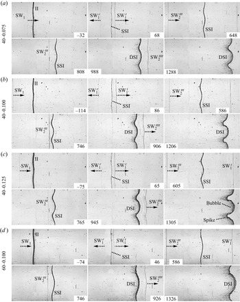
4.1. Flow features and $x$–$t$ diagrams

The wave configurations and the developments of the single-mode interfaces accelerated by two successive shock waves are shown in figure 11. We take the case 40-0.100 as an example to illustrate the detailed process. When the SW$_1$ encounters the initial interface, both disturbed SW$_1^{t}$ and SW$_1^{r}$ are generated. As the SSI moves downward, its amplitude continuously increases induced by baroclinic vorticity and pressure perturbation (86–746 $\mathrm {\mu }$s). The SSI still maintains a quasi-single-mode shape at the arrival of SW$_2^{ttt}$ (746 $\mathrm {\mu }$s), indicating that the perturbation growth is within the linear regime. After the second shock impact, the DSI and the disturbed SW$_2^{tttt}$ can be clearly observed (906 $\mathrm {\mu }$s). For SSS-RMI on a light–heavy interface, the perturbation growth rates induced by the first and second shock waves have the same sign. Therefore, the post-second-shock interface perturbation evolves significantly faster than the pre-second-shock one. As time proceeds, the high-order modes are generated on the interface and the nonlinearity becomes prominent, causing the asymmetry of the interface (906–1206 $\mathrm {\mu }$s). For the cases with a small $k a_0$ (40-0.075) or small $k$ (60-0.100), the asymmetry of the interface is less significant in the late stages. For the case with a large $k a_0$ (40-0.125), the interface becomes highly asymmetrical in the late stages, and both the spike and bubble structures are preliminarily formed (1305 $\mathrm {\mu }$s). These high-quality experiments provide a rare opportunity to examine the linear superposition model and to explore the similarity and difference between single-shocked and double-shocked interfaces in the early nonlinear stages.

Figure 11. Experimental schlieren photographs of the interaction of two successive shock waves with single-mode air–SF$_6$ interfaces: (a) case 40-0.075; (b) case 40-0.100; (c) case 40-0.125; (d) case 60-0.100.

The $x$–$t$ diagrams of shocked interface and shock waves including SW$_1$, SW$_1^{t}$, SW$_1^{r}$, SW$_2^{ttt}$ and SW$_2^{tttt}$ from different experimental runs are shown in figure 10(b), in which the results of cases 40-0.075, 40-0.100, 40-0.125 and 60-0.100 are denoted by black, red, blue and magenta symbols, respectively. The shock waves and shocked interface move almost linearly, indicating that the intensities of shock waves are stable and the interface is not heavily accelerated or decelerated by additional waves other than the SW$_1$ and the SW$_2^{ttt}$ throughout the experiment. Relative to the previous experiments (Buttler et al. Reference Buttler2014a,Reference Buttlerb), a rather ‘clean’ flow field is provided in our experiments, and the interface properties immediately preceding the second shock impact and the temporal evolution of the DSI can be obtained. This provides us an opportunity to theoretically analyse the DSI development.

4.2. Linear and nonlinear growths of single- and double-shocked interfaces

Temporal variations of the pre- and post-second-shock perturbation amplitude (a) for different cases are shown in figure 12(a) in dimensional form, since there is no proper method to simultaneously normalize the pre- and post-second-shock perturbation amplitudes. In all cases, the amplitude of the SSI grows almost linearly with only small fluctuation caused by the start-up process (Richtmyer Reference Richtmyer1960; Yang, Zhang & Sharp Reference Yang, Zhang and Sharp1994; Lombardini & Pullin Reference Lombardini and Pullin2009) and measurement errors. In addition, the pre-second-shock amplitude ($a_2^{-}$) is smaller than 0.1$\lambda$, as shown in table 3. In other words, the perturbation amplitude of the SSI is within the linear growth regime at the arrival of the second shock. In order to predict the perturbation growth rate, the initial amplitude of the interface is crucial. As indicated by Wu, Liu & Xiao (Reference Wu, Liu and Xiao2021), the effective initial amplitude of soap-film interface may be slightly smaller than the initial setting value, which should be caused by the minimum-surface feature of the soap-film interface (Luo et al. Reference Luo, Wang and Si2013). For a minimum surface, the perturbation amplitude on its symmetry plane ($a_0^s$) is smaller than the amplitude on the upper and lower boundaries. In this work, the three-dimensionality of the interface is weak because the ratio of the interface height (6 mm) to its perturbation wavelength is small, and the average value of $a_0$ and $a_0^s$ is approximately considered as the effective initial amplitude $(a_0^{eff} = (a_0+a_0^s)/2)$. After the $a_0^{eff}$ is known, the impulsive model (Richtmyer Reference Richtmyer1960), which has been verified in predicting the linear development of single-mode light–heavy interfaces with small $ka_0$ (Liu et al. Reference Liu, Liang, Ding, Liu and Luo2018), is adopted to predict the linear perturbation growth rate of the SSI ($\dot {a}_1$),

(4.1)\begin{equation} \dot{a}_{1}^t = C_1 k a_0^{eff} A_1^+ u_{ssi}, \end{equation}

where $C_1$ ($= 1 - u_{ssi}/u_{s1}$) is the first shock compression factor. The parameters of the initial interface, and the experimental and theoretical results of $\dot {a}_1$ are listed in table 3. The impulsive model provides a good prediction to the experimental growth rate ($\dot {a}_{1}^e$) because $k a_0^{eff}$ in experiments is small enough.

Figure 12. Temporal variations of pre- and post-second-shock interface perturbation amplitude (a). Comparisons between experimental and theoretical results of dimensionless amplitude of the DSI (b) and dimensionless amplitudes of bubble and spike (c).

Table 3. Experimental and theoretical results of the interaction of successive shock waves with single-mode air–SF$_6$ interfaces.

After the second shock impact, the interface perturbation first grows at an increasing rate due to the start-up process (Richtmyer Reference Richtmyer1960; Yang et al. Reference Yang, Zhang and Sharp1994; Lombardini & Pullin Reference Lombardini and Pullin2009), and then enters a short linear growth period until the nonlinearity becomes pronounced. To predict the linear perturbation growth rate of the post-second-shock interface DSI ($\dot {a}_2$), the linear superposition model proposed by Mikaelian (Reference Mikaelian1985) and Brouillette & Sturtevant (Reference Brouillette and Sturtevant1989) is adopted, which can be described as

(4.2)\begin{equation} \dot{a}_{2}^t = \dot{a}_{1}^t + C_2 k a_2^{-} A_2^{+}{\rm \Delta} u_2, \end{equation}

where $C_2$ ($= 1-{\rm \Delta} u_2 / (u_{s2}^{ttt} - u_{ssi})$) is the second shock compression factor with ${\rm \Delta} u_2=u_{dsi} - u_{ssi}$ being the velocity jump of interface induced by the second shock. The parameters of the pre-second-shock interface, and the experimental and theoretical results of $\dot {a}_2$ are listed in table 3. The linear superposition model slightly overestimates the experimental values. Note that although the SSI perturbation is still within the linear growth regime when the second shock impact occurs, $k a_2^{-}$ is larger than 0.1. Therefore, the high-amplitude effect of pre-second-shock interface should be considered, and the linear superposition model can be modified as

(4.3)\begin{equation} \dot{a}_{2}^{mt} = \dot{a}_1^t + C_{r} C_2 k a_2^{-} A_2^{+}{\rm \Delta} u_2, \end{equation}

where superscript ‘$mt$’ denotes modified theoretical results, $C_{r}$ ($= 1/[1+(k a_2^{-} /3)^{4/3}]$) is the reduction factor introduced by the high-amplitude effect (Dimonte & Ramaprabhu Reference Dimonte and Ramaprabhu2010). The results show that the modified linear superposition model well predicts the linear perturbation growth rate of the post-second-shock interface.

As nonlinearity becomes significant, the perturbation growth rate of the DSI starts to decrease gradually. Up to now, SSS-RMI still lacks rigorous nonlinear theory, and only a few attempts have been made on extending the nonlinear theory of single-shocked interface to double-shocked interface (Karkhanis et al. Reference Karkhanis, Ramaprabhu, Buttler, Hammerberg, Cherne and Andrews2017; Karkhanis & Ramaprabhu Reference Karkhanis and Ramaprabhu2019). These attempts provide an opportunity to explore the similarity and difference in the nonlinear evolution law between single-shocked and double-shocked interfaces. The model proposed by Zhang & Guo (Reference Zhang and Guo2016) (ZG model) has been verified to be applicable for predicting the nonlinear evolution of single-shocked single-mode light–heavy interface with small $k a_0$ (Liu et al. Reference Liu, Liang, Ding, Liu and Luo2018). In this work, the ZG nonlinear model is adopted to predict the nonlinear perturbation growth rate of the DSI, which is written as

(4.4)\begin{equation} \dot{a}{_{b/s}^{ZG}}(t) = \frac{\dot{a}^e_{2}}{1 + \theta_{b/s} k \dot{a}^e_{2} t}, \end{equation}

where

(4.5)\begin{equation} \theta_{b/s}=\frac{3}{4}\frac{(1 \pm A^+_2)(3 \pm A^+_2)}{[3 \pm A^+_2 + \sqrt{2}(1 \pm A^+_2)^{1/2}]} \frac{[4(3 \pm A^+_2) + \sqrt{2}(9 \pm A^+_2)(1 \pm A^+_2)^{1/2}]}{[(3 \pm A^+_2)^2 + 2\sqrt{2}(3\mp A^+_2)(1\pm A^+_2)^{1/2}]}, \end{equation}

with subscripts ‘$b$’ and ‘$s$’ denoting the bubble and spike, respectively. Note that although the SSI is no longer a single-mode interface strictly when the second shock impact occurs, its perturbation is still within the linear growth regime, i.e. the high-order harmonics have negligible effects on the interface development in the weakly nonlinear stages (Liang et al. Reference Liang, Zhai, Ding and Luo2019). Therefore, the ZG model is still applicable. The temporal variations of perturbation amplitude of the DSI in dimensionless form for different cases are shown in figure 12(b). The amplitude and time are normalized as $\alpha = k (a - a_2^*)$ and $\tau = k \dot {a}^e_{2} (t - t^*)$, respectively, where $t^*$ is the moment when the amplitude linear growth of the DSI starts, and $a_2^*$ is the corresponding amplitude of the DSI at $t=t^*$. Only one theoretical line is shown because the predictions for different cases are almost identical. It is shown that the ZG model provides an excellent prediction to the perturbation development of the DSI, i.e. the model for single-shocked interface is capable of predicting the evolution of double-shocked interface. Moreover, the temporal variations of the amplitudes of both the bubble ($\alpha _{b}$) and spike ($\alpha _{s}$) in dimensionless form obtained from experiments and predictions from ZG model are compared, as shown in figure 12(c). Still, the ZG model provides good predictions for the amplitude variations of both the bubble and spike.

4.3. Modal analysis

To further explore the similarity between single-shocked and double-shocked interfaces in the weakly nonlinear evolution stages, modal analysis is performed (Liu et al. Reference Liu, Liang, Ding, Liu and Luo2018; Liang et al. Reference Liang, Zhai, Ding and Luo2019). Firstly, the contours of pre-second-shock interface are extracted from the experiments. Since the pre-second-shock perturbation is still within the linear growth regime, the magnitudes of the third harmonic and the other high-order harmonics relative to that of the first harmonic are very small and negligible, and only the amplitudes of the first and second harmonics are provided,

(4.6)\begin{equation} \left.\begin{gathered} y_{40-0.075} = 2.081 \cos ({kx}) - 0.244 \cos ({2kx}) \cdots. \\ y_{40-0.100} = 2.219 \cos ({kx}) - 0.226 \cos ({2kx}) \cdots. \\ y_{40-0.125} = 3.476 \cos ({kx}) - 0.487 \cos ({2kx}) \cdots. \\ y_{60-0.100} = 2.894 \cos ({kx}) - 0.232 \cos ({2kx}) \cdots. \end{gathered}\right\} \end{equation}

It can be found that the amplitude of the second harmonic is much smaller than that of the first harmonic, i.e. the fundamental mode still dominates, which further proves that the pre-second-shock interface can be approximately regarded as a single-mode one. Then, the contours of the double-shocked interface before the roll-up structure appears are extracted from the schlieren photographs, and Fourier analysis of the interface contours is performed. Figure 13 shows the temporal variations of the amplitudes of the first and second harmonics. For the cases with a small $k a_2^{-}$ (cases 40-0.075, 40-0.100 and 60-0.100), the first harmonic amplitude grows almost linearly whereas the second harmonic amplitude grows very slowly at early times, which are similar to the single-shocked interface with a small $k a_0$ (Liu et al. Reference Liu, Liang, Ding, Liu and Luo2018). When the nonlinearity becomes significant, the growth rate of the first (second) harmonic amplitude becomes smaller (larger). For the case with a relatively large $k a_2^{-}$ (case 40-0.125), the amplitude of the second harmonic grows faster than that in the cases with a small $k a_2^{-}$.

Figure 13. Temporal variations of the perturbation amplitudes of the first and second harmonics. Lines ‘ZS-Small’ denote the predictions of ZS model for the cases 40-0.075, 40-0.100 and 60-0.100, while lines ‘ZS-Large’ denote the predictions of ZS model for the case 40-0.125.

The nonlinear perturbation solutions proposed by Zhang & Sohn (Reference Zhang and Sohn1997) (ZS model) have been proved to be reliable for predicting the amplitude evolutions of the first two harmonics of single-shocked interface with a small $k a_0$ (Liu et al. Reference Liu, Liang, Ding, Liu and Luo2018). The amplitudes of the first two harmonics in ZS model can be written as

(4.7)\begin{gather} a^{(1)} = C_2 a_2^{-} + \dot{a}^e_{2} t - \tfrac{1}{24} (k \dot{a}^e_{2})^2\left\{[4 (A^+_2)^2+1 ] \dot{a}^e_{2} t^3 + 3 C_2 a_2^{-} t^2\right\}, \end{gather}

(4.8)\begin{gather}a^{(2)} ={-} \tfrac{1}{2} A^+_2 k (\dot{a}^e_{2} t )^2 + \tfrac{1}{12} k^3 (\dot{a}^e_{2})^2 [ 4 (A^+_2)^3 (\dot{a}^e_{2})^2 t^4 + 3 A^+_2 (C_2 a_2^{-} t)^2], \end{gather}

where superscript ‘($i$)’ denotes the $i$th harmonic. The predictions from the ZS model are given in figure 13 for comparison. Note that for the cases with a small $k a_2^{-}$, the predictions are almost identical, and only the predictions for the case 40-0.075, denoted as ‘ZS-Small’ in figure 13, are shown to avoid confusion. It can be found that the ZS model reasonably predicts the amplitude developments of the first two harmonics, especially at the early times. For the case 40-0.125 with a large $k a_2^{-}$, the predictions denoted as ‘ZS-Large’ deviate from the experimental counterparts throughout the experiment. As we know, the ZS model was derived based on the assumption that the postshock perturbation amplitude is small. In other words, the accuracy of the ZS model is sensitive to the postshock perturbation amplitude (Zhang & Sohn Reference Zhang and Sohn1997). The post-second-shock perturbation amplitude in the case 40-0.125 is relatively larger ($C_2 k a_2^{-} = 0.478$) than that in other three cases ($C_2 k a_2^{-}\thicksim 0.3$). As a result, the ZS model provides a worse prediction of the experimental results for the case 40-0.125 than other three cases.

In summary, for the SSS-RMI on a light–heavy interface, provided that the second shock impact occurs when the first-shocked interface perturbation is still within the linear growth regime, the linear superposition model, the ZG and ZS models are still reliable to predict the linear, nonlinear and modal evolutions of the double-shocked interface, respectively, when the pre-second-shock interface perturbation is small. When the pre-second-shock perturbation is relatively large, the linear superposition model considering the high-amplitude effect and the ZG model are still valid. However, the ZS model provides relatively poor predictions to the modal evolution. These results indicate that if the first-shocked interface perturbation is within the linear growth regime at the arrival of the second shock, the double-shocked interface behaves similarly to the single-shocked single-mode interface provided that the latter has the same postshock amplitude and the linear growth rate as the former. For double-shocked interface, the second shock provides an additional perturbation velocity field to the original perturbation velocity field introduced by the first shock impact. The validity of the linear superposition model indicates that the linear superposition of these two perturbation velocity fields is satisfied. As a result, a double-shocked interface evolves similarly to a single-shocked interface as long as their postshock amplitudes and linear growth rates are the same.