


1. Introduction
The leading-edge vortex (LEV) is a common flow structure in unsteady aerodynamics, including flapping wings, wind turbines and helicopter rotors. It is well known that the LEV can strongly augment the lift force acting on the lifting surface, as compared to a steady-state flow (McCroskey Reference McCroskey1982; Corke & Thomas Reference Corke and Thomas2015). This phenomenon, commonly known as dynamic stall, results in high lift, even if the angle of attack is far beyond the static stall angle. Although this effect can be advantageous in some applications, for instance, insect manoeuvring at low air speed (Ellington et al. Reference Ellington, Den Berg, Willmott and Thomas1996), it can also be detrimental, leading to high loads and possible material fatigue, as with wind turbine blades bearing cyclic loading (Lin et al. Reference Lin, Lin, Bai and Wang2016). Thus, it is of interest to understand the formation and detachment mechanism of the LEV to take better advantage of dynamic stall or to control its existence and/or strength.
The study of unsteady flow phenomena on wings is often reduced to a two-dimensional case, which is more amenable to analytic, experimental or numerical investigation. For instance, the sinusoidal motion of a profile in steady flow was analytically solved by Theodorsen (Reference Theodorsen1935), assuming attached flow throughout the entire cycle. Sears (Reference Sears1938) and later Atassi (Reference Atassi1984) examined a stationary airfoil placed in a flow with sinusoidal perturbations. These analytic solutions assumed cyclic motion, whereas many experimental studies focused on one-shot motion, i.e. the start-up cycle. Nevertheless, one-shot unsteadiness is of great interest for studying airfoil response to gust-like excitation, as would occur under normal atmospheric conditions. Therefore, one of the aims of the present study is to determine whether there are fundamental differences between one-shot flow fields and cyclic flow fields.
Common to most studies is the choice of dimensionless parameters used to specify the problem. These are the Reynolds number  $(Re = \rho {U_\infty }c/\mu )$, the Strouhal number
  $(St = 2fh/{U_\infty })$ and the reduced frequency
  $(k = {\rm \pi}fc/{U_\infty })$. Here, ρ is the fluid density, U∞ is the free-stream velocity, c is the chord length of the airfoil, μ is the dynamic viscosity, f is the motion frequency and h is half of the maximum plunge height, often measured on the pivot point (Widmann Reference Widmann2015; Eldredge & Jones Reference Eldredge and Jones2019). The main influence of the Reynolds number on dynamic stall is the earlier laminar-to-turbulent transition at higher Re. Baik & Bernal (Reference Baik and Bernal2012) found that, at high Re, the formation of an LEV was suppressed, owing to the unstable boundary layer and rapid transition to the turbulent state. At lower Re, the LEV was reduced to a separated shear layer (Ashraf, Young & Lai Reference Ashraf, Young and Lai2011), although with increasing Re the LEV broke down because of a three-dimensional instability (Visbal Reference Visbal2011; Li et al. Reference Li, Feng, Karbasian, Wang and Kim2019). Baik et al. (Reference Baik, Bernal, Granlund and Michael2012) comprehensively examined the effects of St and k and found that St had a limited influence on the LEV development, whereas an increase in k suppressed the formation of the LEV completely.
Besides the three dimensionless parameters discussed above, LEV development has also been characterized using other dimensionless parameters (Anderson et al. Reference Anderson, Streitlien, Barrett and Triantafyllou1998; Read, Hover & Triantafyllou Reference Read, Hover and Triantafyllou2003; Yu, Wang & Hu Reference Yu, Wang and Hu2013; Tian et al. Reference Tian, Bodling, Liu, Wu, He and Hu2016). Furthermore, Dabiri (Reference Dabiri2009) introduced the optimal vortex formation time to predict the LEV detachment time. The optimal vortex formation time was defined as the maximum circulation that a vortex can reach at the same feeding shear-layer velocity. Rival, Prangemeier & Tropea (Reference Rival, Prangemeier and Tropea2009) confirmed that the optimal formation time was constant in their chosen ranges of parameters. However, Baik et al. (Reference Baik, Bernal, Granlund and Michael2012) also found that the optimal vortex formation time changed under certain conditions. In addition to the optimal vortex formation time, Rival et al. (Reference Rival, Kriegseis, Schaub, Widmann and Tropea2014) postulated that the chord length limited LEV development. Based on these results, Widmann & Tropea (Reference Widmann and Tropea2015) proposed two LEV detachment mechanisms, called ‘bluff-body detachment mechanism’ and ‘boundary-layer eruption detachment mechanism’. The distinction between these mechanisms was whether detachment was triggered by the trailing-edge vortex or the secondary vortex. However, according to the Lagrangian coherent structure results of Huang & Green (Reference Huang and Green2015), Eldredge & Jones (Reference Eldredge and Jones2019) surmised that there might be other LEV detachment mechanisms that were a combination of these two known mechanisms. Therefore, the exact explanation for LEV detachment is still unclear. The present research focuses therefore on the LEV development over a larger test matrix, with the express aim to reveal and examine the different LEV detachment mechanisms.
Parallel to examining LEV detachment, several models for LEV growth have been put forward. Panah, Akkala & Buchholz (Reference Panah, Akkala and Buchholz2015) proposed the vorticity transport budget of LEV circulation, and their analysis utilized properties of the separating shear layer to express the rate of change in LEV circulation. Akkala & Buchholz (Reference Akkala and Buchholz2017) followed this line with experiments designed to assess the accuracy of these influencing factors in two- and three-dimensional cases. Wong, Kriegseis & Rival (Reference Wong, Kriegseis and Rival2013) postulated a two-dimensional vorticity-flux model for the growth of the LEV. In their model, the LEV was approximated as a semicircle at the leading edge, and the feeding shear layer was assumed to be parallel to the effective inflow and was located on the half-cylinder streamline. The results showed good agreement with the LEV circulation during the development phase. Wong & Rival (Reference Wong and Rival2015) further improved the vorticity-flux model by assuming that the shear-layer velocity related with the effective inflow velocity. The LEV circulation growth rate could then be scaled by using the square of the effective inflow velocity.
In summary, these studies provided insight into the LEV development mechanism and the LEV growth. However, there are still numerous unknowns. First, the difference between one-shot and cyclic cases remains unclear, making comparison between such studies questionable. Second, although the maximum effective angle of attack is known to be instrumental in governing dynamic stall, investigations with systematic changes of this parameter are rare. Therefore, in the present study, the influence of maximum effective angle of attack on LEV development under St and k variations for the cyclic case is carefully studied. Finally, an existing LEV growth model could be verified and improved over the investigated parameter range.
2. Experimental apparatus and methods
2.1. Experimental parameters
The experiment was conducted in the water tunnel of Beijing University of Aeronautics and Astronautics (BUAA). The cross-section of the test section is 1000 mm × 1200 mm and the maximum free-stream velocity is 0.5 m s−1. The model profile was a flat plate made of duralumin with sharp leading and trailing edges of angle 30°. It had a chord length of  $c = 120\,{\rm mm}$ and a thickness of 7.2 mm. This is the same profile geometry as used by Widmann & Tropea (Reference Widmann and Tropea2015), with the sharp leading edge ensuring that separation is fixed at the leading edge. The Reynolds number based on the chord length was 24 000 at a free-stream velocity of 200 mm s−1. The turbulence level in the test section of the water tunnel was less than 1.3 %.
A schematic of the experimental set-up is shown in figure 1. One endplate was fixed to the model to suppress the influence of the surface waves. The other endplate was fixed to the bottom of the test section to better approximate two-dimensionality of the flow. The distance between the bottom of the model and the lower endplate was approximately 3 mm. The profile was able to undergo a combined pitching and plunging motion. The pitching motion was driven by a rotating shaft, including a servo motor (Yaskawa SGM7J) and a decelerator (Kamo JFR90). The plunging motion was driven by a servo motor (Yaskawa SGM7J) and a ball screw rod (THK LC-EA-030A). A programmable multi-axes controller (Delta Tau Clipper) was used to control the motion and synchronize with other experimental equipment. The point of rotation was located at the leading edge to avoid the influence of the leading-edge rotation on the flow field.

Figure 1. Schematic diagram of the experimental set-up: (a) end view looking downstream and (b) side view. The yellow arrows indicate the plunging and pitching motion directions.
The present research focused on the influence of the maximum effective angle of attack (αeff,max), the Strouhal number and the reduced frequency. The effective angle of attack is defined using the geometrical angle αgeo(t) undergoing pitching motion and the angle induced by the sinusoidal plunging motion αplunge(t):
 \begin{equation}{\alpha _{eff}}(t) = {\alpha _{geo}}(t) + {\alpha _{plunge}}(t) \approx {\alpha _{eff,max}}\sin (2{\rm \pi} ft),\end{equation}
where
 \begin{equation}{\alpha _{geo}}(t) = {\alpha _{geo,max}}\sin (2{\rm \pi} ft)\end{equation}
and
 \begin{equation}{\alpha _{plunge}}(t) = atan \left( { - \frac{{{U_{plunge}}(t)}}{{{U_\infty }}}} \right) \approx {\alpha _{plunge,max}}\sin (2{\rm \pi} ft).\end{equation}
Here Uplunge(t) is the vertical velocity of the leading edge because of the plunging motion; and αplunge(t) describes the influence of plunging velocity on the effective angle-of-attack variation. An overview of the entire test matrix is given in table 1. The relative phase between the plunging motion and the pitching motion is zero in all cases.
Table 1. Summary of test matrix.

According to this definition, αplunge(t) depends only on the free-stream velocity and the plunging velocity. The constant free-stream velocity resulted in αplunge(t) being adjusted solely by St. Therefore, changing the geometrical angle through pitch changed αeff,max without any other parameter variation. Similarly, the geometrical angle function could be used to keep αeff(t) constant when isolating the influence of St and k. Since αplunge(t) was not strictly a sinusoidal function, the effective angle of attack deviates slightly from the sinusoidal form. Therefore, St was kept smaller than 0.1 to keep this deviation small, as elaborated by Read et al. (Reference Read, Hover and Triantafyllou2003). Time was normalized by the full cycle time (T) to unify the presentation of results from one-shot and cyclic kinematics, using only the first half-cycle for one-shot experiments. Therefore, the upper limit of dimensionless time for the one-shot case is t/T = 0.5. The average effective angle of attack was kept at 0° for all cases. The Strouhal number was chosen either as 0.04 or 0.08. Note that St = 0.08 represents the upper value cited in the literature for obtaining dynamic stall and the lower limit for birds under forward flight conditions (Baik Reference Baik2011). Thus, this range of Strouhal number is of practical significance.
2.2. Particle image velocimetry measurements
The particle image velocimetry (PIV) system comprised a continuous-wave Nd:YAG laser with a power of 8 W and a high-speed complementary metal oxide semiconductor (CMOS) camera (Photron Fastcam SA2/86K-M3) fitted with a Nikon lens (AF 50 mm). Hollow glass beads with median diameter of 20 μm and density of 1.05 g cm−3 were used as tracer particles. The measurement plane was horizontal and positioned at the span midpoint of the flat plate. The magnification of the raw images was approximately 0.17 mm pixel−1 over the entire flow field. Before image processing, the background was subtracted and plate edge identification techniques were used to enhance the particle contrast ratio and to suppress measurement errors arising from the shaded part of the image. A multi-pass iterative Lucas–Kanade method (Champagnat et al. Reference Champagnat, Plyer, Le Besnerais, Leclaire, Davoust and Le Sant2011) was applied to the images to obtain the velocity fields. The size of the final interrogation window was 16 × 16 pixels with 50 % overlap. The spatial resolution of the interrogation window was 2.27 % of the chord length.
For cyclic cases, phase-locked PIV was used. The motion controller sent a trigger signal to the camera whenever the flat plate was in the desired phase. The first five cycles of every set were removed to avoid any start-up effects. A total of 114 cycles for each case with 100 velocity fields per cycle were used to conduct the phase averaging process for the cyclic case. For one-shot cases, time-resolved PIV was used. The sampling frequency was 400 Hz, which corresponds to 2512 velocity fields per cycle. A total of 25 one-shot tests were recorded, and the results were ensemble-averaged to obtain a final velocity field. A local regression low-pass filter was used in the velocity fields of the same phase to remove outliers. Ultimately, the uncertainties of the instantaneous velocity and vorticity were 9.6 mm s−1 and 7 s−1, respectively. It should be mentioned that the cross-correlation coefficient between the velocity components was set to zero, making the actual uncertainty of vorticity less than the computed vorticity uncertainty (Sciacchitano & Wieneke Reference Sciacchitano and Wieneke2016).
2.3. Vortex identification method
To study the LEV evolution, a vortex identification method was necessary to extract the vortex boundary from the vorticity field. The  $\lambda_{ci}$ criterion proposed by Zhou et al. (Reference Zhou, Adrian, Balachandar and Kendall1999) was used in this study to distinguish the vortex. The connected domain with
  $\lambda_{ci}\ge 1\,s^{-1}$ was taken as the limits of a vortex. The chosen identification threshold was able to capture the main vortex structure and avoid the influence of measurement noise inherent in flow velocity values. A polygon line fit to the connected domain was used as the vortex boundary. The vortex circulation was then calculated as a surface integral of vorticity normal to the surface:
 \begin{equation}\varGamma = \int_S {\boldsymbol{\omega }\boldsymbol{\cdot }\boldsymbol{n}\,\textrm{d}S}.\end{equation}
 To reduce the error brought about by interpolation on the measurement mesh, an auxiliary mesh proposed by Onu, Huhn & Haller (Reference Onu, Huhn and Haller2015) was used to calculate  $\lambda_{ci}$. The auxiliary mesh included four points placed symmetrically around each point on the original mesh. These points were used to achieve a higher accuracy in a finite-difference approximation (Onu et al. Reference Onu, Huhn and Haller2015). The spacing of the auxiliary mesh was set to 1 % of the main mesh spacing to increase the accuracy. The value of velocity at the auxiliary mesh was evaluated by spline interpolation method.
Besides the LEV circulation, the LEV position was also important. Therefore, the Γ 1 criterion proposed by Graftieaux, Michard & Grosjean (Reference Graftieaux, Michard and Grosjean2001) was used to find the centre of the LEV. The calculation of Γ 1 at a given point is Γ 1 = ∑sin(θM)/N. Here, θM is the angle between the velocity vector and the radius vector starting from the given point, and N is the number of neighbouring points used in the calculation. The maximum absolute value of Γ 1 within the vortex boundary, determined by the  $\lambda_{ci}$ criterion, was taken as the vortex centre.
3. Results and discussion
3.1. One-shot versus cyclic motion
To compare the flow fields evolving from one-shot or cyclic kinematics, three cases with different αeff,max and St are studied. Figure 2 shows the evolution of normalized vorticity (ωc/U∞) fields for the case of k = 0.3, St = 0.04 and αeff,max = 20°. To equalize the stochastic uncertainty in each measurement, the phase averaging of the cyclic case was limited to 25 cycles, and the same number of one-shot repetitions was used. The flow structure between the two cases is very similar. At t/T = 0.15, the negative vorticity is concentrated around the leading edge. The LEV cannot be easily distinguished from the leading-edge shear layer until about t/T = 0.25. Meanwhile, positive vorticity develops behind the leading edge, representing the formation of secondary structures between the leading-edge shear layer and the LEV. At t/T = 0.35, the connection between the LEV and the leading-edge shear layer is weak, indicating that the LEV no longer accumulates vorticity from the feeding shear layer. By the end of the downstroke, the LEV has passed beyond the trailing edge.

Figure 2. Normalized vorticity fields and velocity vectors at different dimensionless times for (a) one-shot and (b) cyclic kinematics (k = 0.3, St = 0.04 and αeff,max = 20°).
Figure 3 illustrates a similar comparison, but for a lower maximum effective angle of attack: k = 0.3, St = 0.04 and αeff,max = 16°. Again, the flow field developments for the two kinematic cases are very similar; however, differences from the αeff,max = 20° case (figure 2) are apparent. The size and the strength of LEV for αeff,max = 16° are smaller and the secondary structure with positive vorticity is almost imperceptible.

Figure 3. Normalized vorticity fields and velocity vectors at different dimensionless times for (a) one-shot and (b) cyclic kinematics (k = 0.3, St = 0.04 and αeff,max = 16°).
A quantitative comparison of profile kinematic influences on the flow field development is presented in figure 4, where the vortex centre trajectories are compared for various test matrix cases in the same dimensionless time interval. First, the vortex trajectories of different motion kinematics are quite similar. This means that the motion kinematics has limited influence on the LEV development. Second, the trajectories remain similar for different St, confirming the findings of Baik et al. (Reference Baik, Bernal, Granlund and Michael2012). Third, it can be found that the LEV generated with a higher maximum effective angle of attack convects further downstream during the same dimensionless time. In conclusion, the flow topologies of one-shot and cyclic kinematics are very similar. The influence of dimensionless parameters on the flow structure development is also similar for the one-shot and cyclic cases. Therefore, in further analyses of flow field development, results from the cyclic experiments have been used.

Figure 4. The LEV centre trajectories shown in the plate coordinate system for the two motion kinematics over the dimensionless time interval 0.12 < t/T < 0.35 for various test matrix cases.
3.2. Influence of maximum effective angle of attack
Figure 5 shows the normalized vorticity fields under different maximum effective angles of attack. In the case of αeff,max = 12°, only a recirculation zone is observed on the suction side of the flat plate, with no visible secondary structure. There is no rotational centre identifiable in the flow field. With increasing maximum effective angle of attack to αeff,max = 16°, the LEV exhibits higher circulation and positive vorticity appears below the LEV on the plate and behind the leading edge. For αeff,max = 20° and 24°, the LEV becomes much stronger in circulation and the secondary vortex forms much earlier. Moreover, a trailing-edge vortex (TEV) forms when the LEV detaches from the shear layer and passes the trailing edge. The formation of the TEV is independent of the secondary vortex. These phenomena imply that an increase of the maximum effective angle of attack facilitates the formation of vortex structures during plate motion. Because the LEV is a typical flow structure associated with dynamic stall, the following discussion now focuses on the cases of αeff,max = 16°–24°.

Figure 5. Normalized vorticity fields and velocity vector development with time for different maximum effective angles of attack, (a) αeff,max = 12°, (b) αeff,max = 16°, (c) αeff,max = 20° and (d) αeff,max = 24°, under St = 0.04 and k = 0.3.
A more graphic representation of the flow topology development is presented in figure 6, showing the normalized near-wall tangential velocity along the plate (ut/U∞) as a function of dimensionless time. The near-wall velocity is taken as the mean of the three wall-adjacent PIV interrogation areas. In this representation, the reattachment point of the LEV on the plate, xrp, corresponding to a half-saddle point, is indicated by the black line separating positive and negative near-wall velocities. This plot has been presented for St = 0.04, k = 0.3 and three maximum effective angles of attack αeff,max = 16°, 20° and 24°. The flow field topology and development are similar for all cases. The secondary vortex is easily distinguishable as positive velocities between the separating shear layer and the LEV for the cases of αeff,max = 20° and 24°. The positive velocity is much weaker for the case of αeff,max = 16°; this suggests that there is no strong secondary vortex during the downstroke under this condition. Furthermore, the reattachment point of the LEV reaches the trailing edge earlier for the higher maximum effective angle of attack, as will be discussed below.

Figure 6. (a) Diagram of LEV reattachment point. (b–d) Normalized surface tangential velocity (ut/U∞) for different maximum angles of attack: (b) αeff,max = 16°, (c) αeff,max = 20° and (d) αeff,max = 24°, under St = 0.04 and k = 0.3. The black line is the trajectory of the LEV reattachment point.
Figure 7 shows the normalized circulation of the LEV (ΓLEV/cU∞) and secondary vortex (ΓSV/cU∞) against dimensionless time. The vertical dashed lines indicate the time when the LEV reattachment point reaches the trailing edge. For αeff,max = 16°, the LEV circulation reaches its maximum far before the reattachment point reaches the trailing edge. The time difference between these two moments reduces with increasing maximum effective angle of attack. For αeff,max = 24°, the LEV circulation just starts to decrease when the reattachment point reaches the trailing edge.

Figure 7. Normalized LEV and secondary vortex circulation developments for different maximum effective angles of attack. The vertical dashed lines represent the time when the LEV reattachment point reaches the trailing edge.
The secondary vortex circulation of αeff,max = 16° remains low throughout the entire half-cycle and is only detectable after the LEV circulation reaches its maximum. This suggests that the secondary vortex does not significantly influence the development of the LEV. For the cases of αeff,max = 20° and 24°, the secondary vortex is much stronger. The secondary vortex continues to grow even after the LEV circulation reaches its maximum. The simultaneous increase of both the LEV and the secondary vortex circulation implies that the formation and growth of the secondary vortex is dependent on the strength of the LEV. The continuous increase of secondary vortex circulation suggests that the backflow induced by the LEV may be a key influencing factor.
In both the LEV detachment mechanisms proposed by Rival et al. (Reference Rival, Kriegseis, Schaub, Widmann and Tropea2014) and Widmann & Tropea (Reference Widmann and Tropea2015), namely boundary-layer eruption detachment and bluff-body detachment, respectively, the time when the reattachment point behind the LEV reaches the trailing edge and the time when secondary vortex is formed are important criteria. The unique feature of boundary-layer eruption detachment is that the formation of a secondary vortex and the decrease of LEV circulation occur earlier in time than when the reattachment point behind the LEV reaches the trailing edge. For bluff-body detachment, the LEV circulation starts to decrease after the LEV reaches the trailing edge, without a strong influence of the secondary vortex. Accordingly, the cases investigated in the present study belong to the boundary-layer eruption category because the LEV circulation starts to decrease before the reattachment point reaches the trailing edge. However, differences do exist. For αeff,max = 16°, the LEV circulation starts to decrease in the absence of a visible secondary vortex and a TEV. For αeff,max = 20° and 24°, the LEV circulation continues to increase, while not directly decreasing after the formation of the secondary vortex. Therefore, it cannot be concluded that the LEV detachment is based solely on the growth of the secondary vortex. Another LEV detachment mechanism may exist for the present experimental cases, especially for the case of αeff,max = 16°.
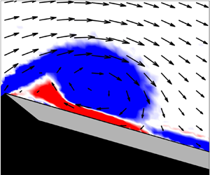
Before continuing the discussion, the concept of a separated shear-layer angle is introduced. Figure 8(a) illustrates the method used to calculate the shear-layer angle. First, points displaying the highest negative vorticity are identified in the shear layer (marked green in figure 8a). Then a linear fit to these points is used, whereby the number of points used (between 7 and 10) is chosen according to which fit results in the largest correlation coefficient R 2. The angle between the fitting line and the plate surface is taken as the shear-layer angle.

Figure 8. (a) Principle for computing the shear-layer angle from the normalized vorticity field. The green points are those with highest negative vorticity. The yellow line is the fitted line used to represent the leading-edge shear layer. (b–d) The development of shear-layer angle for k = 0.3 and St = 0.04 with different maximum angles of attack: (b) αeff,max = 16°, (c) αeff,max = 20° and (d) αeff,max = 24°.
Figure 8(b–d) shows the evolution of shear-layer angle for different maximum effective angles of attack. The magnitude of the error bars depends on the standard deviation of shear-layer angle fluctuations, observed as fluctuations of phase-averaged values. All curves exhibit a similar development and, accordingly, three phases can be identified: the growth phase, the steady phase and the decreasing phase. These three phases are demarcated in figure 8(b–d) using a grey background.
In considering these three phases of shear-layer angle development, the final phase, i.e. the decreasing phase, is rather obviously a consequence of LEV detachment from the feeding shear layer. For the case of αeff,max = 16°, the third phase begins around the time when the LEV reaches the trailing edge, while the third phase begins after the LEV reaches the trailing edge for the cases of αeff,max = 20° and 24°.
To give possible explanations for the growth phase and the steady phase, the change of the LEV boundary with phase is examined. Figure 9(a) depicts the measured boundary and the vortex centre of the LEV at different dimensionless times in the plate coordinate system of the case of k = 0.3, St = 0.04 and αeff,max = 24°. This boundary has been fitted at each time to an ellipse form. The ratio of minor axis to major axis for the fitting ellipse, namely the inverse of the aspect ratio of the LEV (1/ARLEV), is calculated and shown in figure 9(b). The gradual increase of 1/ARLEV in the growth phase clearly shows that the shape of the LEV changes from elliptic to circular. The overall trend for 1/ARLEV develops in a similar time frame as the shear-layer angle. The small deviation is because the shear-layer angle depends not only on the LEV shape deformation, but also on the movement of the vortex centre. However, the simultaneous variation suggests that the change of the LEV shape is the main reason for the shear-layer angle phase transition.

Figure 9. (a) The fitted elliptic boundary of the LEV at different times for the case of k = 0.3, St = 0.04 and αeff,max = 24°. (b) The variation of the inverse of the aspect ratio of the LEV, which is defined as the ratio between the minor axis and the major axis for the fitted boundary of the LEV. The red dashed line denotes the time when the first phase transits to the second phase. (c,d) Schematic diagrams of the evolution of the LEV in (c) the growth phase and (d) the steady phase of shear-layer angle development.
In the growth phase (t/T < 0.2), the vertical growth of the LEV, including the change of shape and the movement of the vortex centre, results in a higher angle of the leading-edge shear layer, as shown in figure 9(c). This explains the first phase observed in figure 8(b–d). In the steady phase (0.2 < t/T < 0.4), the LEV grows not only vertically, but also in the chord-wise direction. The balance between the growth in the vertical and chord-wise directions of the LEV results in an almost constant value of the leading-edge shear-layer angle, as shown in figure 9(d).
The time at which the shear-layer angle changes from the growth phase to the steady phase is denoted ‘transition time’. According to Doligalski, Smith & Walker (Reference Doligalski, Smith and Walker1994), the movement of the vortex occurs because of the boundary-layer response, when the vortex Reynolds number is large enough. Hence, the transition time represents the time when boundary-layer response starts to interrupt the LEV development. Figure 10 shows a high-resolution depiction of the vorticity field near the leading edge for cases of αeff,max = 16° and 24° around the transition time. This representation reveals that different secondary structures exist at the transition time, which are the different types of boundary-layer response to the LEV. For the case of αeff,max = 16°, a positive vorticity layer under the LEV erupts just after the transition time, as the yellow circle shows. Akkala & Buchholz (Reference Akkala and Buchholz2017) also found this positive vorticity layer in their high-resolution result. The vorticity-layer eruption is a consequence of the downstream convection of the LEV. For the case of αeff,max = 24°, an obvious secondary vortex replaces the vorticity-layer eruption as the dominant influencing structure. Therefore, it can be concluded that the growth of the secondary structure increases the convective velocity of the LEV downstream. Thus, different secondary structures play the role of interrupting the LEV development for different maximum effective angles of attack.

Figure 10. Normalized vorticity field with velocity vectors near the leading edge of (a) αeff,max = 16°, t/T = 0.20, (b) αeff,max = 16°, t/T = 0.22, (c) αeff,max = 24°, t/T = 0.19, and (d) αeff,max = 24°, t/T = 0.21, under k = 0.3 and St = 0.04.
As a consequence of the no-slip condition on the plate surface, it is reasonable to assume that a stronger LEV creates more positive vorticity in the near-wall vorticity layer. Therefore, the surface tangential velocity at a position that is below the vortex centre, ui, is calculated, as shown in figure 11(a). Figure 11(b) shows the induced velocity development at different αeff,max values. The leading-edge shear-layer transition times are also shown by vertical dashed lines. The induced velocity increases with an increase in the maximum effective angle of attack. This suggests that the strong LEV in the case of high αeff,max would induce a strong vorticity layer, which finally produces the secondary vortex to interrupt the LEV development. For the case of αeff,max = 16°, the weak LEV can only induce vorticity-layer eruption from the vorticity layer.

Figure 11. (a) Schematic diagram of the LEV induced velocity. (b) The normalized induced velocity for different maximum effective angles of attack. The vertical dashed lines mark the leading-edge shear-layer transition time.
Furthermore, the critical vortex Reynolds number, which is the vortex Reynolds number (Reν = Γ/2πν, where ν is the kinematic viscosity) of the LEV at the transition time is calculated, as listed in table 2. The critical vortex Reynolds number in the case of αeff,max = 16° is far smaller than that in other cases. The nearly same transition time means that the time for LEV uninterrupted development is similar. Because the LEV development is determined by the inflow condition, it can be assumed that the αeff(t) function has the main influence on the transition time. However, this assumption still needs further research. Following the approach of Doligalski et al. (Reference Doligalski, Smith and Walker1994), the vortex Reynolds number is used to distinguish the viscous response provoked by a vortex in the near-wall flow. Therefore, the different vortex Reynolds numbers observed at the transition time determine which kind of secondary structure, namely the vorticity-layer eruption or the secondary vortex, will interrupt the LEV development and lead to LEV detachment.
Table 2. Shear-layer angle transition time and corresponding critical vortex Reynolds number.

The observed flow topology exhibits different characteristics for different maximum effective angles of attack. Three scenarios, shown in figure 12, can be concluded from the previous analysis, namely a quasi-steady development scenario, a vorticity-layer eruption scenario and a secondary vortex formation scenario, which correspond to the cases of αeff,max = 12°, αeff,max = 16° and αeff,max = 20°–24°, respectively. In the quasi-steady development scenario, a single recirculation zone is the main flow feature and no obvious LEV can be observed. With the vorticity-layer eruption scenario, despite the formation of the LEV, the vortex strength is only sufficient to provoke vorticity-layer eruption. In the secondary vortex formation scenario, the LEV is sufficiently strong to induce the formation of a secondary vortex. To quantitatively determine which of the latter two scenarios will occur, the vortex Reynolds number at the transition time of the shear-layer angle is a good indicator.

Figure 12. Three different flow topology scenarios with increase in the maximum effective angle of attack: (a) quasi-steady development scenario, (b) vorticity-layer eruption scenario, and (c) secondary vortex formation scenario.
3.3. Discussion on flow topology scenarios
Subsequent to the results discussed above, the influence of k and St on the flow topology scenario is also studied in figures 13 and 14. Figure 13 shows the development of the normalized vorticity field at different values of St at k = 0.3 and αeff,max = 24°. The flow topology for different St values does not exhibit significant differences. The LEV circulation variations for different St values are also similar to each other, as shown in figure 15(a). The secondary vortex is observed during the LEV development. Baik et al. (Reference Baik, Bernal, Granlund and Michael2012) indicated that St had a limited influence on the LEV development in the larger range (St > 0.1). Therefore, the same flow topology scenario at different St values with constant αeff,max is expected.

Figure 13. Normalized vorticity field and velocity vector development with time for different St: (a) St = 0.04 and (b) St = 0.08 under k = 0.3 and αeff,max = 24°.

Figure 14. Normalized vorticity field and velocity vector development with time for different k: (a) k = 0.3, (b) k = 0.45 and (c) k = 0.6 under St = 0.04 and αeff,max = 16°.

Figure 15. Normalized LEV circulation development for (a) different Strouhal numbers and (b) different reduced frequencies.
The normalized vorticity fields at different values of k at St = 0.04 and αeff,max = 16° are shown in figure 14. With an increase in k, the LEV development is significantly postponed, which is also validated by LEV circulation variation, as shown in figure 15(b). The time when the reattachment point of the LEV reaches the trailing edge is delayed with an increase in the reduced frequency. Although the LEV for higher k has a higher vorticity, the extent of the LEV is much smaller. The secondary structure at t/T = 0.35 for k = 0.6 is stronger than the one for k = 0.3. The distinct secondary structure for the case of higher reduced frequency indicates that it contributes to the detachment of LEV from the feeding shear layer.
The critical vortex Reynolds number is used to quantitatively distinguish the flow topology scenario at different St and k values. Figure 16 shows the critical vortex Reynolds numbers under different experimental parameters. Two values, a higher one at approximately 4500 for the secondary vortex formation and a lower one at approximately 2500 for the vorticity-layer eruption, can be clearly identified in the results. This indicates that the flow topology development is mainly dependent on the maximum effective angle of attack. Although k would postpone the development of LEV, the flow topology scenario does not change with the same maximum effective angle of attack.

Figure 16. Flow topology scenario and the corresponding critical vortex Reynolds number for all cases studied.
3.4. LEV growth model
A simplified model describing the growth of circulation in the LEV is now introduced. In previous models, the mass flow from the feeding shear layer into the vortex determined the vortex growth rate (Kaden Reference Kaden1931). Using the same assumption, Sattari et al. (Reference Sattari, Rival, Martinuzzi and Tropea2012) and Wong et al. (Reference Wong, Kriegseis and Rival2013) proposed a model for the steady flux of vorticity from the shear layer into a two-dimensional vortex. These theories and results are modified in the present model. First, a new coordinate system fixed on the plate, with the origin at the leading edge, is introduced. Second, the outer contour of the LEV is approximated as a circular arc projecting from the leading edge, as depicted in figure 17(a). Third, the shear layer is assumed to be oriented tangential to this circular arc at the leading edge. Fourth, the velocity on the vortex outer contour is assumed to be constant, following Sattari et al. (Reference Sattari, Rival, Martinuzzi and Tropea2012). Then the circulation of the LEV can be expressed as
 \begin{equation}\varGamma (t) \approx 2{\alpha _{eff}}(t)R(t){U_b}(t),\end{equation}
where the R(t) is the radius of the arc and Ub(t) is the velocity at the vortex outer boundary. Since the velocity Ub(t) is assumed constant along the arc, then it can take the value of the effective inflow velocity at the leading edge, Ueff(t). The Ueff(t) is the vector sum of the free-stream velocity U∞ and the plunge velocity Uplunge(t). The model now requires specification of the radius R(t). Figure 6 indicates that the LEV reattachment point moves along the chord linearly in time; hence, the LEV radius can also be assumed to grow linearly in time, i.e. R(t) = Kt. Here, K is a constant which represents the growth rate of the radius. Thus, the LEV circulation can be expressed as
 \begin{equation}\varGamma (t) \approx 2Kt{\alpha _{eff}}(t){U_{eff}}(t).\end{equation}
This model can only be applied after the onset of an LEV; thus the onset time of the LEV, tonset, is required. For this, a polynomial fitting of the LEV circulation is used to locate the onset time of the LEV, as was also used by Buchner et al. (Reference Buchner, Soria, Honnery and Smits2018). This approach can be illustrated graphically, as shown in figure 17(b).

Figure 17. Diagram of (a) LEV outer vortex boundary approximated using a circular arc and (b) polynomial fitting of the LEV circulation, yielding the LEV onset time.
In this manner, the evolution of the normalized LEV circulation,  ${\varGamma ^\ast }(t) = \varGamma /2c{\alpha _{eff}}(t){U_{eff}}(t)$, relative to the normalized time from LEV onset, (t − tonset)/T, can be obtained for all cases, as shown in figure 18. A linear relationship between the normalized circulation and dimensionless time, namely Γ* ~ K*t/T, can be found with St, k and αeff variations. Here, K* represents the dimensionless growth rate of the vortex radius, which is normalized based on the chord length and the full cycle time. It is suggested that all cases presented here have similar normalized growth rates. Consequently, the effective inflow velocity Ueff and the effective angle of attack αeff can be considered as two key parameters in determining the LEV growth. The most important improvement of this model is the quantitative connection between effective inflow condition, Ueff and αeff, and LEV circulation development. This reveals that the common plate motion parameters, including St, k and αeff, influence the dynamic stall characteristics by changing the effective inflow condition. The plates with pure plunging motion, pure pitching motion, and combined pitching and plunging motion can all use this model to describe the LEV circulation development. Besides, this model shows that the radius of the vortex increases linearly with time. This assumption helps to simplify the calculation of the radius and vortex strength during plate motion.

Figure 18. The normalized LEV circulation as a function of cycle time from LEV onset.
4. Conclusion
The flow around a pitching and plunging flat plate has been experimentally studied for both one-shot and cyclic motion kinematics and over wide ranges of maximum effective angle of attack, Strouhal number and reduced frequency. The results indicate that there is very little difference in flow field topology between the one-shot and cyclic cases.
The LEV development for different maximum effective angles of attack under cyclic motion is then studied in more detail, leading to three different topological scenarios, depending on the magnitude of the maximum effective angle of attack. The quasi-steady development scenario corresponds to a single recirculation zone as the main flow characteristic. The vorticity-layer eruption and the formation of a secondary vortex are the main features of the two other scenarios. The influence of these secondary structures on LEV development is reflected in the variation of the leading-edge shear-layer angle. In addition, it is found that the tangential velocity induced by the LEV on the plate determines the different secondary structures. Because the vortex circulation is based on the velocity distribution at the vortex boundary, the vortex Reynolds number, which normalizes the vortex circulation at the shear-layer angle transition time, is studied. It is found to be an efficient method to distinguish between the vorticity-layer eruption and secondary vortex formation scenarios. These two scenarios occur at a critical vortex Reynolds number of around 2500 and 4500, respectively. According to a comprehensive variation of St and k, the vortex Reynolds number at the shear-layer angle transition time is demonstrated to be mainly dependent on the maximum effective angle of attack.
Finally, a simplified model for the LEV growth is proposed. This model is based on the transport of vorticity into the vortex through the shear layer. The velocity is assumed to be constant at the vortex outer boundary. The outer boundary is approximated by a circular arc, projecting from the leading edge. The simplified model reveals that the LEV growth is primarily determined by the effective inflow velocity and the effective angle of attack. It describes well the experimental results of circulation growth over time for all cases. Based on this model, it is possible to predict the LEV evolution with more studies on the prediction of the LEV onset time. It should be noted that the proposed model is based on flow over a flat plate. The sharp leading edge ensures that the separation point is fixed at the leading edge during motion, which is conducive for the growth of the LEV. However, the movement of the separation point when the leading edge is not sharp, like the leading edge of an airfoil, would delay the formation of the LEV (Rival et al. Reference Rival, Kriegseis, Schaub, Widmann and Tropea2014). The onset time of the LEV would also be delayed in this case. Future study of different leading-edge geometries is suggested to clarify this behaviour.
Acknowledgements
This work was supported by the Sino-German Research Project (no. GZ 1280), by the National Natural Science Foundation of China (nos 11722215, 11721202) and by the Deutsche Forschungsgemeinschaft under Project TR 194/55-1.
Declaration of interests
The authors report no conflict of interest.


