


1 Introduction
Flapping flight is a common mode of insect locomotion which is characterized by complex and unsteady aerodynamic phenomena. As visualized in tethered (Jensen Reference Jensen1956) and untethered flight (Fry, Sayaman & Dickinson Reference Fry, Sayaman and Dickinson2003) measurements, the flow field around a flapping insect wing at intermediate Reynolds numbers (
 $50\leqslant Re\leqslant 1000$
) is highly unsteady and vortical. Periodic flapping motion generates larger time-averaged lift and drag forces than those of an equivalent translating airfoil (Lentink & Dickinson Reference Lentink and Dickinson2009), suggesting that unsteady mechanisms are important to insect flight at small scales.
$50\leqslant Re\leqslant 1000$
) is highly unsteady and vortical. Periodic flapping motion generates larger time-averaged lift and drag forces than those of an equivalent translating airfoil (Lentink & Dickinson Reference Lentink and Dickinson2009), suggesting that unsteady mechanisms are important to insect flight at small scales.
In several studies (Dickinson & Gotz Reference Dickinson and Gotz1993; Ellington et al. Reference Ellington, Van Den Berg, Willmott and Thomas1996; Dickinson, Lehmann & Sane Reference Dickinson, Lehmann and Sane1999) researchers have found that the most important feature of flapping flight involves the development of a strong leading edge vortex (LEV) during the wing translation phase. The LEV corresponds to a low-pressure region on the wing upper surface, and it is responsible for the observed high lift. As shown in both experimental and computational studies (Wang, Birch & Dickinson Reference Wang, Birch and Dickinson2004; Bos et al. Reference Bos, Lentink, Van Oudheusden and Bijl2008), the growth and shedding of the LEV is sensitive to the flapping kinematics. In addition, the interaction between shed vortices and a flapping airfoil significantly influences the flapping kinematics and dynamics (Alben & Shelley Reference Alben and Shelley2005). Using a dynamically scaled robotic wing, Dickinson et al. (Reference Dickinson, Lehmann and Sane1999) characterized unsteady phenomena such as rotational circulation and delayed stall. Wang et al. (Reference Wang, Birch and Dickinson2004) corroborated this observation through constructing and solving 2D computational fluid dynamics (CFD) models. Recent experimental studies (Lentink & Dickinson Reference Lentink and Dickinson2009) and computational work have focused on subtle phenomena such as LEV stability, wing–wing interactions and 3D flow patterns (Thielicke & Stamhuis Reference Thielicke and Stamhuis2015). Computationally intensive 3D CFD simulation (Zheng, Hedrick & Mittal Reference Zheng, Hedrick and Mittal2013) was developed to study unsteady 3D effects. Meanwhile, computationally inexpensive quasi-steady blade element (Sane & Dickinson Reference Sane and Dickinson2001) models were also proposed to explore how kinematic parameters influence manoeuvrability and flight stability (Wang & Chang Reference Wang and Chang2013).
These advances in the understanding of flapping-wing aerodynamics, together with inspiration observed from nature, have led to the design and successful flight of numerous flapping-wing micro-air vehicles (MAVs) (Lentink, Jongerius & Bradshaw Reference Lentink, Jongerius and Bradshaw2010; Keennon et al. Reference Keennon, Klingebiel, Won and Andriukov2012; Ma et al. Reference Ma, Chirarattananon, Fuller and Wood2013). To reduce mechanical complexity, all of these vehicles employ passive wing pitching mechanics to regulate the wing angle of attack. In nature, passive pitching is also observed in some insect flight from measurements of the torsional wave propagation direction along the wing span (Ennos Reference Ennos1988).
While an analysis based on aerodynamic power expenditure has shown the feasibility of passive wing pitching (Bergou, Xu & Wang Reference Bergou, Xu and Wang2007), there have been very few studies on passive fluid–wing interaction due to a number of experimental and modelling challenges. From an experimental perspective, the study of fluid–wing interactions at the insect scale requires the building of millimetre-scale flapping-wing devices and the resolution of time varying forces at micro-Newton levels. From a theoretical perspective, the adoption of a classical quasi-steady model to predict passive wing rotation requires careful analysis because aerodynamic torque estimation sensitively depends on wing geometry and kinematics. Further, numerical simulations are often more accurate yet computationally expensive; hence, it is important to compare the accuracy of quasi-steady and numerical models against experimental measurements with different kinematic and morphological inputs. A previous study (Whitney & Wood Reference Whitney and Wood2010) addressed the experimental challenges by designing and testing an insect-scale robotic flapper under various kinematic inputs. However, that study did not use particle image velocimetry (PIV) techniques and numerical simulations to study flow structures surrounding a flapping wing. Consequently, the authors were not able to quantify the influence of design parameters such as hinge stiffness and flapping amplitude on flapping efficiency. The interplay between passive pitching and force generation has a profound influence on hovering efficiency and manoeuvrability. Here, we conduct a detailed study of the influence of kinematic parameters on passive pitching and force generation.
Our research on passive wing pitching dynamics fits into the broad category of fluid mechanics studies on flexible airfoils. In recent years numerous studies have explored fluid–wing interactions through modelling hinge compliance or wing flexibility. Zhao et al. (Reference Zhao, Huang, Deng and Sane2010) explored the effects of trailing edge flexibility on force generation through testing a scaled-up wing in an oil tank. Nakata & Liu (Reference Nakata and Liu2011) performed a similar study through numerical simulations. Kang & Shyy (Reference Kang and Shyy2012) compared the effects of hinge compliance and wing flexibility through numerical simulation and found that hinge compliance has a large influence on flapping efficiency. Zhang, Liu & Lu (Reference Zhang, Liu and Lu2010) explored the passive pitching influence on a self-propelled airfoil. Thiria & Godoy-Diana (Reference Thiria and Godoy-Diana2010) and Ramananarivo, Godoy-Diana & Thiria (Reference Ramananarivo, Godoy-Diana and Thiria2011) explored the competing influences of system resonance and wing flexibility. An interesting paper by Spagnolie et al. (Reference Spagnolie, Moret, Shelley and Zhang2010) combined experimental and numerical approaches; however, the experiments were performed in a much larger Reynolds number (
 $Re$
) regime (
$Re$
) regime (
 $10^{5}$
). While these studies offer insights to the underlying fluid mechanics, they do not include comparison between measurement and numerical modelling at the insect scale (
$10^{5}$
). While these studies offer insights to the underlying fluid mechanics, they do not include comparison between measurement and numerical modelling at the insect scale (
 $50\leqslant Re\leqslant 1000$
). Here, we combine quasi-steady modelling, numerical modelling and at-scale experiments to study flapping-wing flight with passive pitching. This approach allows us to identify strengths and weaknesses of quasi-steady and numerical models. More importantly, these comparison studies allow us to make predictions about design parameter values that lead to efficient flapping motion.
$50\leqslant Re\leqslant 1000$
). Here, we combine quasi-steady modelling, numerical modelling and at-scale experiments to study flapping-wing flight with passive pitching. This approach allows us to identify strengths and weaknesses of quasi-steady and numerical models. More importantly, these comparison studies allow us to make predictions about design parameter values that lead to efficient flapping motion.
With the goal of investigating the relationship between force generation and wing passive pitching, we mainly use quasi-steady models and 2D CFD simulations to explore fluid–wing interactions. The main difference between a 2D translating wing and a 3D revolving wing is that in steady state the LEV remains stably attached on the revolving wing over a much longer distance. On a 3D revolving wing, the pressure gradient between the wing tip and the wing root causes spanwise flow to stabilize the LEV. However, unlike a rotor, an insect wing accelerates, decelerates and reverses in every flapping period. As shown in the particle velocimetry results of Cheng et al. (Reference Cheng, Roll, Liu, Troolin and Deng2014), insect flapping wings shed vortices in the wake, and the associated flow structures differ from those of rotary propellers. In the cases we study here, the stroke amplitude to wing chord ratio is small (between 2 and 5), which suggests that delayed vortex shedding caused by wing rotation is not significant. Further, several previous studies (Wang et al. Reference Wang, Birch and Dickinson2004; Bos et al. Reference Bos, Lentink, Van Oudheusden and Bijl2008) have demonstrated that 2D simulations can give reasonable approximations of insect flight. To investigate the effects of 3D phenomena on lift and drag generation, we implement a 3D CFD solver and compare 2D and 3D simulations.
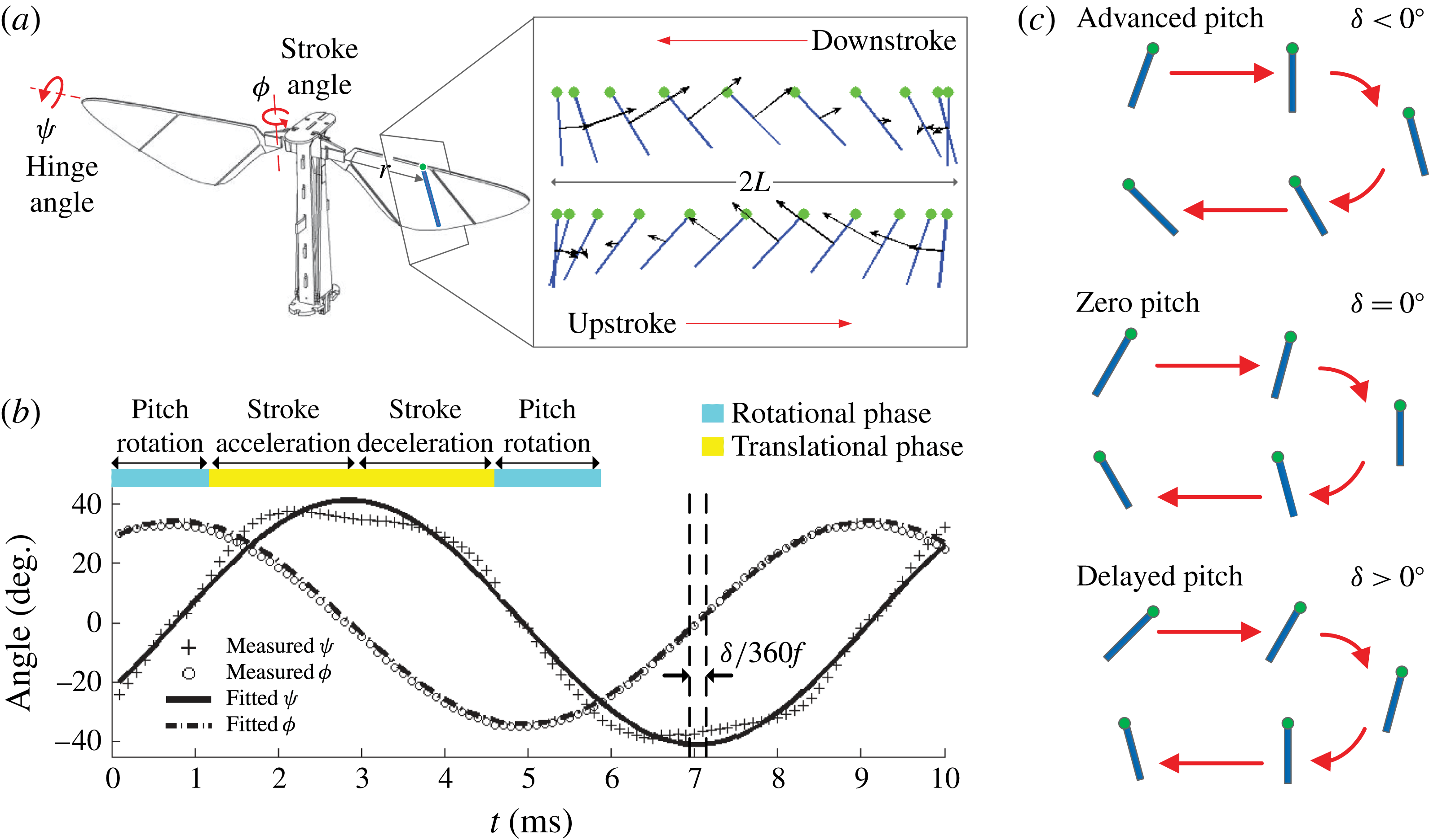
Figure 1. Flapping-wing kinematics. (a) Wing stroke (
 ${\it\phi}$
) and hinge (
${\it\phi}$
) and hinge (
 ${\it\psi}$
) motion. The motion of a thin rectangular segment along the wing chord is projected onto a 2D plane. (b) Experimental kinematics extraction shows that stroke and hinge motion are well approximated by pure sinusoids. A flapping period is broken down into translational (yellow) and rotational (blue) phases. (c) Passive wing pitch rotation is described by a phase shift parameter
${\it\psi}$
) motion. The motion of a thin rectangular segment along the wing chord is projected onto a 2D plane. (b) Experimental kinematics extraction shows that stroke and hinge motion are well approximated by pure sinusoids. A flapping period is broken down into translational (yellow) and rotational (blue) phases. (c) Passive wing pitch rotation is described by a phase shift parameter
 ${\it\delta}$
, with
${\it\delta}$
, with
 ${\it\delta}<0^{\circ }$
corresponding to advanced pitch and
${\it\delta}<0^{\circ }$
corresponding to advanced pitch and
 ${\it\delta}>0^{\circ }$
corresponding to delayed pitch.
${\it\delta}>0^{\circ }$
corresponding to delayed pitch.
In this paper, we take an integrated and multifidelity approach towards investigating the relationship between wing kinematics and lift force generation. We fabricate a millimetre-scale piezoelectric flapping device with passive wing pitching and measure time varying lift forces and flow quantities. The experimental study is complemented by a modified quasi-steady model to identify favourable flapping kinematics and optimal hinge stiffness values. A high-fidelity numerical model is also applied to a number of wing kinematics to analyse unsteady mechanisms such as LEV dynamics. We show that our quasi-steady model gives good estimates of hinge stiffnesses that allow favourable flapping kinematics. Comparison with experiments shows that our numerical model accurately describes fluid–wing interactions and surrounding flow structures. Our study further quantifies the relationship between wing pitch rotation, LEV strength and mean lift generation. The results presented here are of broad interest to biologists, physicists and engineers interested in insect flight and the design of micro-aerial vehicles.
The outline of this paper is as follows. Section 2 introduces a modified quasi-steady model and explains the numerical solver implementation. Section 3 describes the experimental set-up for measuring forces and flow field quantities. Section 4 compares quasi-steady model predictions, numerical simulations and experimental measurements. Finally, concluding remarks are given in § 5.
2 Quasi-steady modelling and numerical simulation
2.1 Flapping kinematics
During hovering, insect wings typically have three degrees of freedom (Ellington Reference Ellington1984). However, the motion that is normal to the stroke plane (i.e. ‘stroke plane deviation’) is usually very small. In our robotic design (as shown in figure 1
a), we make the simplifying approximation that the kinematics of a flapping wing has two degrees of freedom: stroke and hinge rotations (i.e. wing pitching). The experimental set-up allows us to control the frequency and amplitude of the stroke motion, while the hinge rotation is passively controlled by aerodynamic and inertial torques and hinge compliance. As shown in figure 1(b), the experimental measurement shows that the hinge motion is close to a pure sinusoid, where the amplitude of the second harmonic component is approximately 19 % that of the fundamental harmonic. While this small but noticeable component does not have a large effect on force production, it offers interesting insight into the role of insect steering muscles. In a previous study Dickson et al. measured the flapping kinematics of a flying Drosophila (figure 9 of Dickson, Straw & Dickinson (Reference Dickson, Straw and Dickinson2008)). Compared with our experimental measurement, we observe similar stroke (
 ${\it\phi}(t)$
) and pitch (
${\it\phi}(t)$
) and pitch (
 ${\it\psi}(t)$
) motion. In particular,
${\it\psi}(t)$
) motion. In particular,
 ${\it\psi}(t)$
has noticeable flattened peaks in both measurements. This similarity implies that fruit fly steering muscles may function similarly to a linear torsional spring.
${\it\psi}(t)$
has noticeable flattened peaks in both measurements. This similarity implies that fruit fly steering muscles may function similarly to a linear torsional spring.
The stroke and hinge motion can be approximated as
 $$\begin{eqnarray}\displaystyle & \displaystyle {\it\phi}={\it\phi}_{max}\cos (2{\rm\pi}ft), & \displaystyle\end{eqnarray}$$
 $$\begin{eqnarray}\displaystyle & \displaystyle {\it\psi}={\it\psi}_{max}\sin (2{\rm\pi}ft+{\it\delta}), & \displaystyle\end{eqnarray}$$
 ${\it\phi}_{max}$
is the stroke amplitude,
${\it\phi}_{max}$
is the stroke amplitude,
 ${\it\psi}_{max}$
is the hinge amplitude,
${\it\psi}_{max}$
is the hinge amplitude,
 $f$
is the flapping frequency and
$f$
is the flapping frequency and
 ${\it\delta}$
is the relative phase. Figure 1(c) illustrates that
${\it\delta}$
is the relative phase. Figure 1(c) illustrates that
 ${\it\delta}<0^{\circ }$
corresponds to advanced pitch rotation and
${\it\delta}<0^{\circ }$
corresponds to advanced pitch rotation and
 ${\it\delta}>0^{\circ }$
corresponds to delayed pitch rotation. In quasi-steady blade element models and 2D CFD models, the angular stroke motion is approximated by the translational motion of a thin blade element located a distance
${\it\delta}>0^{\circ }$
corresponds to delayed pitch rotation. In quasi-steady blade element models and 2D CFD models, the angular stroke motion is approximated by the translational motion of a thin blade element located a distance
 $r$
from the wing root. As shown in figure 1(a), the amplitude of the wing chord translational motion is given by
$r$
from the wing root. As shown in figure 1(a), the amplitude of the wing chord translational motion is given by
 $L=r{\it\phi}_{max}$
. We choose
$L=r{\it\phi}_{max}$
. We choose
 $r$
to be the wing midspan because PIV studies show that the circulation is strongest near midspan (Birch & Dickinson Reference Birch and Dickinson2003) and the effect of wing tip vortical flow near midspan is small. A detailed discussion of wing driver design and kinematics measurement will be given in §§ 3.1 and 3.3.
$r$
to be the wing midspan because PIV studies show that the circulation is strongest near midspan (Birch & Dickinson Reference Birch and Dickinson2003) and the effect of wing tip vortical flow near midspan is small. A detailed discussion of wing driver design and kinematics measurement will be given in §§ 3.1 and 3.3.
As shown in figure 1(b), the flapping period can be further decomposed into the translational phase and the rotational phase. The translational phase refers to the wing motion during midstroke at an approximately constant angle of attack. The rotational phase occurs during wing pitch reversal at the transition between down and up strokes. During this phase, the wing stroke velocity is small and hence lift and drag forces are smaller than those in the translational phase. As a consequence, the lift peak in the translational phase is called the primary lift peak whereas the lift peak observed during wing reversal is called the secondary lift peak. We discuss the influence of the kinematic parameters on the primary and secondary lift peaks in § 4.
2.2 Quasi-steady modelling
We develop a quasi-steady model to predict the aerodynamic forces and passive wing pitching at midstroke given different driving frequencies, stroke amplitudes and wing hinge stiffnesses. We assume that the relative phase shift
 ${\it\delta}$
is small and both stroke and hinge motions are purely sinusoidal. Consequently, we need to predict
${\it\delta}$
is small and both stroke and hinge motions are purely sinusoidal. Consequently, we need to predict
 ${\it\psi}_{max}$
,
${\it\psi}_{max}$
,
 $F_{L}$
and
$F_{L}$
and
 $F_{D}$
given
$F_{D}$
given
 $f$
,
$f$
,
 ${\it\phi}_{max}$
, wing shape and hinge stiffnesses. Here
${\it\phi}_{max}$
, wing shape and hinge stiffnesses. Here
 $F_{L}$
and
$F_{L}$
and
 $F_{D}$
are defined as the lift and drag force, respectively.
$F_{D}$
are defined as the lift and drag force, respectively.
Our quasi-steady model is based on the blade element model used in numerous previous studies of insect flight (Dickinson et al. Reference Dickinson, Lehmann and Sane1999; Sane & Dickinson Reference Sane and Dickinson2001; Whitney & Wood Reference Whitney and Wood2010). The blade element model states that the instantaneous force on a translating wing chord is proportional to the local velocity squared. The total force on a translating wing is given by the integral along the wing span direction:
 $$\begin{eqnarray}F_{i}(t)=\frac{1}{2}C_{i}({\it\alpha}(t)){\it\rho}\int _{x_{r}}^{x_{r}+R}u^{2}(r,t)c(r)\,\text{d}r,\end{eqnarray}$$
where
 ${\it\rho}$
is the air density,
${\it\rho}$
is the air density,
 $u(r,t)$
is the local wing chord velocity,
$u(r,t)$
is the local wing chord velocity,
 $x_{r}$
is the wing root location,
$x_{r}$
is the wing root location,
 $c(r)$
is the local chord length and
$c(r)$
is the local chord length and
 $i$
stands for either lift (
$i$
stands for either lift (
 $L$
) or drag (
$L$
) or drag (
 $D$
). The force coefficients
$D$
). The force coefficients
 $C_{i}$
are functions of the angle of attack
$C_{i}$
are functions of the angle of attack
 ${\it\alpha}$
, which is defined as
${\it\alpha}$
, which is defined as
 ${\it\alpha}={\rm\pi}/2-{\it\psi}$
. Equation (2.2) is derived from thin-airfoil theory under the assumption of steady inviscid external flow without flow separation. In addition, it also assumes that the instantaneous force generation only depends on the instantaneous motion of the flapping insect wing but not the unsteadiness of the surrounding fluid. Consequently, extra terms such as added mass, wake capture and rotational acceleration need to be added to (2.2) to account for unsteady effects during wing rotation. Sane and Dickinson showed that using experimentally measured coefficients
${\it\alpha}={\rm\pi}/2-{\it\psi}$
. Equation (2.2) is derived from thin-airfoil theory under the assumption of steady inviscid external flow without flow separation. In addition, it also assumes that the instantaneous force generation only depends on the instantaneous motion of the flapping insect wing but not the unsteadiness of the surrounding fluid. Consequently, extra terms such as added mass, wake capture and rotational acceleration need to be added to (2.2) to account for unsteady effects during wing rotation. Sane and Dickinson showed that using experimentally measured coefficients
 $C_{L}$
and
$C_{L}$
and
 $C_{D}$
the quasi-steady model can give accurate time-averaged force predictions (figure 3 in Sane & Dickinson (Reference Sane and Dickinson2001)).
$C_{D}$
the quasi-steady model can give accurate time-averaged force predictions (figure 3 in Sane & Dickinson (Reference Sane and Dickinson2001)).
This quasi-steady model assumes fully prescribed kinematics; however, in our study we need to solve a coupled fluid–wing system because the wing pitching is passive. As shown in a previous study (Whitney & Wood Reference Whitney and Wood2010), the coefficients of the added terms change considerably as the wing shape and kinematics vary in passive pitching experiments. Hence, adoption of the full quasi-steady model to analyse wing passive pitching may be subject to excessive overfitting. Consequently, we only use the translational term (2.2) of the quasi-steady model to estimate the aerodynamic force and to predict the passive pitching at midstroke. In (2.2) the lift and drag coefficients
 $C_{L}({\it\alpha})$
and
$C_{L}({\it\alpha})$
and
 $C_{D}({\it\alpha})$
are substituted with Dickson’s dynamically scaled measurements (figure 5 in Dickson et al. (Reference Dickson, Straw and Dickinson2008)). The local wing chord velocity
$C_{D}({\it\alpha})$
are substituted with Dickson’s dynamically scaled measurements (figure 5 in Dickson et al. (Reference Dickson, Straw and Dickinson2008)). The local wing chord velocity
 $u(r)$
equals
$u(r)$
equals
 $2{\rm\pi}fr$
at midstroke, where
$2{\rm\pi}fr$
at midstroke, where
 $f$
is the flapping frequency and
$f$
is the flapping frequency and
 $r$
is the spanwise position.
$r$
is the spanwise position.
In addition to invoking (2.2) we need to solve for the angle of attack
 ${\it\alpha}$
simultaneously at midstroke. If we assume that the relative phase shift
${\it\alpha}$
simultaneously at midstroke. If we assume that the relative phase shift
 ${\it\delta}$
is small and both stroke and hinge motions are purely sinusoidal, then
${\it\delta}$
is small and both stroke and hinge motions are purely sinusoidal, then
 ${\it\alpha}$
is a minimum at midstroke. We can solve for
${\it\alpha}$
is a minimum at midstroke. We can solve for
 ${\it\alpha}_{min}$
by imposing Euler’s angular momentum equation:
${\it\alpha}_{min}$
by imposing Euler’s angular momentum equation:
 $$\begin{eqnarray}\sum {\bf\tau}_{i}=\unicode[STIX]{x1D644}\boldsymbol{\cdot }{\bf\omega}+{\bf\omega}\times (\unicode[STIX]{x1D644}\boldsymbol{\cdot }{\bf\omega}),\end{eqnarray}$$
where
 $\sum {\bf\tau}_{i}$
is the sum of external torques,
$\sum {\bf\tau}_{i}$
is the sum of external torques,
 $\unicode[STIX]{x1D644}$
is the moment of inertia tensor and
$\unicode[STIX]{x1D644}$
is the moment of inertia tensor and
 ${\bf\omega}$
is the angular velocity of the wing. The spanwise component of (2.3) is
${\bf\omega}$
is the angular velocity of the wing. The spanwise component of (2.3) is
 $$\begin{eqnarray}K{\it\psi}-(F_{L}\cos {\it\alpha}+F_{D}\sin {\it\alpha})R_{cop}=I_{xx}\ddot{{\it\alpha}}+(I_{yy}-I_{zz})\dot{{\it\phi}}^{2}\cos {\it\psi}\sin {\it\psi},\end{eqnarray}$$
where
 $K$
represents the hinge stiffness,
$K$
represents the hinge stiffness,
 $R_{cop}$
is the mean chordwise centre of pressure and
$R_{cop}$
is the mean chordwise centre of pressure and
 $I_{xx}$
is the effective rotational moment of inertia considering added mass contributions from the surrounding fluid. We obtain
$I_{xx}$
is the effective rotational moment of inertia considering added mass contributions from the surrounding fluid. We obtain
 $I_{xx}$
,
$I_{xx}$
,
 $I_{yy}$
and
$I_{yy}$
and
 $I_{zz}$
from the CAD modelling software SolidWorks (SolidWorks, 2013, Troy, MI), and we adopt the added mass corrections from Whitney & Wood (Reference Whitney and Wood2010). Here, we ignore the contribution of the centre of mass to the rotational axis. This approximation is justified in the supplementary material available at http://dx.doi.org/10.1017/jfm.2016.35. The value of the hinge stiffness
$I_{zz}$
from the CAD modelling software SolidWorks (SolidWorks, 2013, Troy, MI), and we adopt the added mass corrections from Whitney & Wood (Reference Whitney and Wood2010). Here, we ignore the contribution of the centre of mass to the rotational axis. This approximation is justified in the supplementary material available at http://dx.doi.org/10.1017/jfm.2016.35. The value of the hinge stiffness
 $K$
is given in § 4.1 and details of wing planforms and wing inertial properties are given in appendix A.
$K$
is given in § 4.1 and details of wing planforms and wing inertial properties are given in appendix A.
Equations (2.2) and (2.4) form a coupled system that gives lift, drag and angle of attack predictions based on kinematic and morphological inputs. While parameters such as the hinge stiffness and wing inertia are straightforward to calculate, the centre of pressure coefficient
 $R_{cop}$
is difficult to model. A quasi-steady model based on thin-airfoil theory always places
$R_{cop}$
is difficult to model. A quasi-steady model based on thin-airfoil theory always places
 $R_{cop}$
at the quarter-chord position, but this prediction does not hold for flapping flight due to flow separation and unsteady effects. Through experiments, we find that
$R_{cop}$
at the quarter-chord position, but this prediction does not hold for flapping flight due to flow separation and unsteady effects. Through experiments, we find that
 $R_{cop}$
is a strong function of wing shape and angle of attack. For a particular wing planform,
$R_{cop}$
is a strong function of wing shape and angle of attack. For a particular wing planform,
 $R_{cop}({\it\alpha})$
needs to be measured first.
$R_{cop}({\it\alpha})$
needs to be measured first.
With the assumption that the wing stroke and pitch motion are purely sinusoidal,
 $R_{cop}({\it\alpha})$
can be calculated using measured kinematics at wing midstroke. We can substitute the kinematic parameters into (2.4) and obtain
$R_{cop}({\it\alpha})$
can be calculated using measured kinematics at wing midstroke. We can substitute the kinematic parameters into (2.4) and obtain
 $$\begin{eqnarray}R_{cop}=\frac{K({\rm\pi}/2-{\it\alpha}_{min})-4{\rm\pi}^{2}f^{2}I_{xx}({\rm\pi}/2-{\it\alpha}_{min})-4{\rm\pi}^{2}f^{2}(I_{yy}-I_{zz}){\it\phi}_{max}^{2}\cos {\it\alpha}_{min}\sin {\it\alpha}_{min}}{F_{L}\cos {\it\alpha}_{min}+F_{D}\sin {\it\alpha}_{min}}.\end{eqnarray}$$
By varying driving inputs and measuring the corresponding kinematic parameters, we can obtain
 $R_{cop}({\it\alpha})$
for a range of
$R_{cop}({\it\alpha})$
for a range of
 ${\it\alpha}$
. To evaluate the performance of a particular wing, we first run several experiments to measure the hinge kinematics. Then we solve for
${\it\alpha}$
. To evaluate the performance of a particular wing, we first run several experiments to measure the hinge kinematics. Then we solve for
 $R_{cop}({\it\alpha})$
as a function of
$R_{cop}({\it\alpha})$
as a function of
 ${\it\alpha}$
using (2.2) and (2.5). After
${\it\alpha}$
using (2.2) and (2.5). After
 $R_{cop}({\it\alpha})$
is computed, (2.2) and (2.4) can be used to simultaneously predict lift, drag and wing pitching kinematics for other driving conditions and hinge stiffnesses. Due to the assumption that
$R_{cop}({\it\alpha})$
is computed, (2.2) and (2.4) can be used to simultaneously predict lift, drag and wing pitching kinematics for other driving conditions and hinge stiffnesses. Due to the assumption that
 ${\it\delta}$
is small, (2.4) and (2.5) are only invoked at midstroke.
${\it\delta}$
is small, (2.4) and (2.5) are only invoked at midstroke.
In summary, our proposed quasi-steady model assumes purely sinusoidal stroke and pitch motion with small phase shift
 ${\it\delta}$
. By adopting Dickson’s experimentally obtained lift and drag coefficients and imposing angular momentum balance, the model solves for lift, drag and angle of attack at wing midstroke. This quasi-steady model is easy to evaluate and provides useful predictions for flapping-wing experiments. The functional form of
${\it\delta}$
. By adopting Dickson’s experimentally obtained lift and drag coefficients and imposing angular momentum balance, the model solves for lift, drag and angle of attack at wing midstroke. This quasi-steady model is easy to evaluate and provides useful predictions for flapping-wing experiments. The functional form of
 $C_{L}({\it\alpha})$
is very close to
$C_{L}({\it\alpha})$
is very close to
 $\sin (2{\it\alpha})$
, which implies that maximum lift can be achieved when the minimum angle of attack is approximately
$\sin (2{\it\alpha})$
, which implies that maximum lift can be achieved when the minimum angle of attack is approximately
 $45^{\circ }$
. Given a wing planform, flapping frequency and stroke amplitude, we can use this quasi-steady model to estimate the appropriate hinge stiffness that leads to the desired hinge motion. Here, we refer to the process of finding the optimal hinge stiffness for the desired pitching motion as wing characterization. From an experimental perspective, this model reduces the number of wing hinge fabrication and flapping tests needed to achieve the desired performance. However, the model ignores unsteady effects that may be crucial for certain kinematic inputs. In addition, the model also requires experimental measurement of
$45^{\circ }$
. Given a wing planform, flapping frequency and stroke amplitude, we can use this quasi-steady model to estimate the appropriate hinge stiffness that leads to the desired hinge motion. Here, we refer to the process of finding the optimal hinge stiffness for the desired pitching motion as wing characterization. From an experimental perspective, this model reduces the number of wing hinge fabrication and flapping tests needed to achieve the desired performance. However, the model ignores unsteady effects that may be crucial for certain kinematic inputs. In addition, the model also requires experimental measurement of
 $R_{cop}$
for every wing planform. We discuss its accuracy and shortcomings in § 4.1.
$R_{cop}$
for every wing planform. We discuss its accuracy and shortcomings in § 4.1.
2.3 Numerical simulation with fully prescribed kinematics
In passive flapping experiments kinematic parameters such as
 ${\it\phi}_{max}$
,
${\it\phi}_{max}$
,
 ${\it\psi}_{max}$
and
${\it\psi}_{max}$
and
 ${\it\delta}$
are interdependent. Consequently, it is difficult to explore the influence of a single parameter. A numerical model based on fully prescribed kinematic inputs can be used to study parameter dependence and influence. Here, we implement a numerical model that solves the incompressible Navier–Stokes equation. Our computational model assumes a 2D flat plate of dimensions
${\it\delta}$
are interdependent. Consequently, it is difficult to explore the influence of a single parameter. A numerical model based on fully prescribed kinematic inputs can be used to study parameter dependence and influence. Here, we implement a numerical model that solves the incompressible Navier–Stokes equation. Our computational model assumes a 2D flat plate of dimensions
 $90~{\rm\mu}\text{m}\times 3~\text{mm}$
flapping in air with kinematics described in § 2.1. The wing chord dimension is chosen based on wings used in experiments. The incompressible Navier–Stokes equation and the corresponding boundary conditions that govern the flapping motion are
$90~{\rm\mu}\text{m}\times 3~\text{mm}$
flapping in air with kinematics described in § 2.1. The wing chord dimension is chosen based on wings used in experiments. The incompressible Navier–Stokes equation and the corresponding boundary conditions that govern the flapping motion are
 $$\begin{eqnarray}\displaystyle & \displaystyle {\it\rho}\frac{\partial \boldsymbol{u}}{\partial t}+{\it\rho}(\boldsymbol{u}\boldsymbol{\cdot }\boldsymbol{{\rm\nabla}})\boldsymbol{u}=-\boldsymbol{{\rm\nabla}}p+{\it\mu}{\rm\nabla}^{2}\boldsymbol{u}, & \displaystyle\end{eqnarray}$$
 $$\begin{eqnarray}\displaystyle & \displaystyle \boldsymbol{{\rm\nabla}}\boldsymbol{\cdot }\boldsymbol{u}=0, & \displaystyle\end{eqnarray}$$
 $$\begin{eqnarray}\displaystyle & \displaystyle \boldsymbol{u}|_{wing}=(u,v)_{wing}, & \displaystyle\end{eqnarray}$$
 $$\begin{eqnarray}\displaystyle & \displaystyle p|_{\infty }=0, & \displaystyle\end{eqnarray}$$
 ${\it\rho}$
is the fluid density,
${\it\rho}$
is the fluid density,
 ${\it\mu}$
is the fluid viscosity,
${\it\mu}$
is the fluid viscosity,
 $\boldsymbol{u}=(u,v)$
is the fluid velocity field and
$\boldsymbol{u}=(u,v)$
is the fluid velocity field and
 $p$
is the pressure field that enforces the incompressibility condition. The fluid speed on the wing surface is equal to the wing velocity, and the pressure at far field is set to be 0. In our computations, the range of Reynolds numbers is between 50 and 1000.
$p$
is the pressure field that enforces the incompressibility condition. The fluid speed on the wing surface is equal to the wing velocity, and the pressure at far field is set to be 0. In our computations, the range of Reynolds numbers is between 50 and 1000.
To solve this partial differential equation (PDE), we implement a numerical solver using the nodal discontinuous Galerkin finite element method (FEM-DG). The solver is implemented on a moving Cartesian coordinate system. The computational Delaunay triangulation mesh is generated by the open source package DistMesh (Persson & Strang Reference Persson and Strang2004), and we specify smaller mesh elements around wing leading and trailing edges to resolve flow–structure details. The mesh radius is chosen to be 15 times the wing chord to reduce artificial boundary effects. The solution inside each mesh element is interpolated using fifth-order Lagrange polynomials, and the mesh consists of approximately 4000 elements.
The structure of this solver is based on the method developed in Hesthaven & Warburton (Reference Hesthaven and Warburton2007). The temporal scheme is solved using the second-order backward Adams–Bashforth method, and the spatial scheme is separated into three steps that individually treat nonlinear advection, pressure field contribution and viscous correction. The first step is solved explicitly whereas the last two steps are formulated as implicit Poisson and Helmholtz equations respectively. For the pressure field, we impose Neumann boundary conditions along the wing surface and Dirichlet boundary conditions on the mesh boundary. For the velocity fields, we impose Dirichlet boundary conditions along the wing surface and Neumann boundary conditions on the mesh boundary. The size of the time step
 ${\rm\Delta}t$
is determined using the method in Hesthaven & Warburton (Reference Hesthaven and Warburton2007) to satisfy stability conditions. In our simulation,
${\rm\Delta}t$
is determined using the method in Hesthaven & Warburton (Reference Hesthaven and Warburton2007) to satisfy stability conditions. In our simulation,
 ${\rm\Delta}t$
is in the range of
${\rm\Delta}t$
is in the range of
 $0.4{-}0.6~{\rm\mu}\text{s}$
, which means that each flapping period consists of approximately 17 000 time steps. The 2D CFD model validation is given in appendix B.
$0.4{-}0.6~{\rm\mu}\text{s}$
, which means that each flapping period consists of approximately 17 000 time steps. The 2D CFD model validation is given in appendix B.
Given the fluid velocity field and the pressure field we can compute the force per unit length and torque per unit length on the wing segment by integrating the stress tensor along the wing surface:
 $$\begin{eqnarray}\boldsymbol{f}=\int _{wing}\hat{\boldsymbol{n}}\boldsymbol{\cdot }{\bf\sigma}\,\text{d}l,\quad \boldsymbol{t}=\int _{wing}\boldsymbol{r}\times (\hat{\boldsymbol{n}}\boldsymbol{\cdot }{\bf\sigma})\,\text{d}l,\end{eqnarray}$$
where
 $\hat{\boldsymbol{n}}$
is the local surface normal. Lower case letters represent quantities per unit length. We can expand the stress tensor and arrive at equations for the lift and drag forces as follows:
$\hat{\boldsymbol{n}}$
is the local surface normal. Lower case letters represent quantities per unit length. We can expand the stress tensor and arrive at equations for the lift and drag forces as follows:
 $$\begin{eqnarray}\displaystyle & \displaystyle f_{L}=-\int _{wing}\left(-pn_{y}+{\it\nu}{\it\rho}\frac{\partial u}{\partial y}n_{x}+{\it\nu}{\it\rho}\frac{\partial v}{\partial x}n_{y}+2{\it\nu}{\it\rho}\frac{\partial v}{\partial y}n_{y}\right)\,\text{d}l, & \displaystyle\end{eqnarray}$$
 $$\begin{eqnarray}\displaystyle & \displaystyle f_{D}=-\int _{wing}\left(-pn_{x}+2{\it\nu}{\it\rho}\frac{\partial u}{\partial x}n_{x}+{\it\nu}{\it\rho}\frac{\partial v}{\partial x}n_{y}+{\it\nu}{\it\rho}\frac{\partial u}{\partial y}n_{y}\right)\,\text{d}l. & \displaystyle\end{eqnarray}$$
We can further compute the instantaneous chordwise lift and drag coefficients as
 $$\begin{eqnarray}\displaystyle & \displaystyle C_{L}=\frac{f_{L}}{{\textstyle \frac{1}{2}}{\it\rho}u^{2}c}, & \displaystyle\end{eqnarray}$$
 $$\begin{eqnarray}\displaystyle & \displaystyle C_{D}=\frac{f_{D}}{{\textstyle \frac{1}{2}}{\it\rho}u^{2}c}, & \displaystyle\end{eqnarray}$$
 $u$
is the instantaneous chord leading edge velocity and
$u$
is the instantaneous chord leading edge velocity and
 $c$
is the local wing chord length. Finally, we can relate to the experimental measurements by substituting the computed
$c$
is the local wing chord length. Finally, we can relate to the experimental measurements by substituting the computed
 $C_{L}$
and
$C_{L}$
and
 $C_{D}$
into (2.2). The time-averaged lift and drag forces can be computed by integrating (2.2) over a flapping period.
$C_{D}$
into (2.2). The time-averaged lift and drag forces can be computed by integrating (2.2) over a flapping period.
Figure 2(a) illustrates the moving wing coordinates
 $({\it\xi},{\it\eta})$
, the inertial coordinates
$({\it\xi},{\it\eta})$
, the inertial coordinates
 $(x,y)$
, the definition of
$(x,y)$
, the definition of
 $f_{L}$
and
$f_{L}$
and
 $f_{D}$
with respect to the stroke velocity
$f_{D}$
with respect to the stroke velocity
 $\boldsymbol{u}$
and the fluid torque
$\boldsymbol{u}$
and the fluid torque
 ${\it\tau}_{f}$
with respect to the wing leading edge. Figure 2(b) shows an enlarged image of the computational mesh.
${\it\tau}_{f}$
with respect to the wing leading edge. Figure 2(b) shows an enlarged image of the computational mesh.

Figure 2. The set-up of the 2D FEM-DG numerical solver. (a) A moving wing coordinate is defined by
 $({\it\xi},{\it\eta})$
and an inertial coordinate is defined by
$({\it\xi},{\it\eta})$
and an inertial coordinate is defined by
 $(x,y)$
. The direction of lift force always points upward, and the direction of drag force is always opposite to the stroke velocity
$(x,y)$
. The direction of lift force always points upward, and the direction of drag force is always opposite to the stroke velocity
 $\boldsymbol{u}$
. (b) A zoomed-in image of the triangulated computational mesh. Finer elements are generated near the leading and trailing edges to resolve flow details. The mesh tip geometry in (b) facilitates convergence and does not compromise lift and drag accuracy.
$\boldsymbol{u}$
. (b) A zoomed-in image of the triangulated computational mesh. Finer elements are generated near the leading and trailing edges to resolve flow details. The mesh tip geometry in (b) facilitates convergence and does not compromise lift and drag accuracy.
2.4 Numerical simulation with partially prescribed kinematics
While the quasi-steady model in § 2.2 predicts the wing pitch
 ${\it\psi}_{max}$
, it is limited by the assumption that the phase shift
${\it\psi}_{max}$
, it is limited by the assumption that the phase shift
 ${\it\delta}$
is small. We can relax this assumption by formulating a coupled fluid–mesh numerical model to study passive pitch rotation. At each computation time step, the incompressible Navier–Stokes equation is solved to obtain the flow field and the pressure field. The computed flow exerts fluid torque on a passive polymer hinge that is modelled as a torsional spring. Consequently, we can formulate an ordinary differential equation (ODE) that models the wing pitching:
${\it\delta}$
is small. We can relax this assumption by formulating a coupled fluid–mesh numerical model to study passive pitch rotation. At each computation time step, the incompressible Navier–Stokes equation is solved to obtain the flow field and the pressure field. The computed flow exerts fluid torque on a passive polymer hinge that is modelled as a torsional spring. Consequently, we can formulate an ordinary differential equation (ODE) that models the wing pitching:
 $$\begin{eqnarray}i_{xx}\ddot{{\it\psi}}+k{\it\psi}+ml\ddot{X}\cos {\it\psi}+{\it\tau}_{f}=0,\end{eqnarray}$$
where
 $k$
is the hinge stiffness and
$k$
is the hinge stiffness and
 $i_{xx}$
is the principal moment of inertia in the spanwise direction. The term
$i_{xx}$
is the principal moment of inertia in the spanwise direction. The term
 $ml\ddot{X}\cos {\it\psi}$
corresponds to the effect of stroke acceleration on the offset centre of mass. In this term
$ml\ddot{X}\cos {\it\psi}$
corresponds to the effect of stroke acceleration on the offset centre of mass. In this term
 $m$
is the wing mass per unit length and
$m$
is the wing mass per unit length and
 $l$
is the centre of mass offset to the rotation axis. For the simulation shown in § 4.2.3 this term is ignored because its effect is small compared with the unsteady 3D contribution. The derivation of (2.10) is given in the supplementary material. This ODE is solved using a forward Euler method. This coupled PDE–ODE system allows us to numerically model passive hinge motion and to study fluid–wing interaction.
$l$
is the centre of mass offset to the rotation axis. For the simulation shown in § 4.2.3 this term is ignored because its effect is small compared with the unsteady 3D contribution. The derivation of (2.10) is given in the supplementary material. This ODE is solved using a forward Euler method. This coupled PDE–ODE system allows us to numerically model passive hinge motion and to study fluid–wing interaction.
In (2.10),
 $i_{xx}$
is computed with respect to the wing leading edge using the parallel axis theorem and does not include an added mass correction as it is in the quasi-steady model. Since this is a 2D numerical model,
$i_{xx}$
is computed with respect to the wing leading edge using the parallel axis theorem and does not include an added mass correction as it is in the quasi-steady model. Since this is a 2D numerical model,
 $i_{xx}$
and
$i_{xx}$
and
 $k$
are normalized to quantities per unit length. Here,
$k$
are normalized to quantities per unit length. Here,
 $i_{xx}$
is normalized by the wing span as
$i_{xx}$
is normalized by the wing span as
 $i_{xx}=I_{xx}/R$
. In our experimental set-up the flapping motion has a 3D rotational component, which means that choosing the equivalent hinge stiffness in 2D simulation is challenging. A wing chord that is near the wing tip experiences larger aerodynamic and inertial forces. Since the wing leading edge position varies along the wing span, the chordwise centre of rotation also changes along the wing span. This shift of the chordwise centre of rotation has a noticeable effect on torque estimation; hence, it is important to adjust for 3D effects. The normalized hinge stiffness value needs to be a function of wing chord spanwise location and wing shape;
$i_{xx}=I_{xx}/R$
. In our experimental set-up the flapping motion has a 3D rotational component, which means that choosing the equivalent hinge stiffness in 2D simulation is challenging. A wing chord that is near the wing tip experiences larger aerodynamic and inertial forces. Since the wing leading edge position varies along the wing span, the chordwise centre of rotation also changes along the wing span. This shift of the chordwise centre of rotation has a noticeable effect on torque estimation; hence, it is important to adjust for 3D effects. The normalized hinge stiffness value needs to be a function of wing chord spanwise location and wing shape;
 $k$
should have the form of
$k$
should have the form of
 $$\begin{eqnarray}k=\frac{1}{{\it\beta}}\left(\frac{r}{R}\right)^{2}\frac{K}{w},\end{eqnarray}$$
where
 $K$
is the wing hinge stiffness,
$K$
is the wing hinge stiffness,
 $w$
is the hinge width,
$w$
is the hinge width,
 $(r/R)^{2}$
gives the spanwise scaling and
$(r/R)^{2}$
gives the spanwise scaling and
 ${\it\beta}$
is a dimensionless number that accounts for wing shape and other 3D effects. In the comparison between experiments and simulations, we experiment with several values of
${\it\beta}$
is a dimensionless number that accounts for wing shape and other 3D effects. In the comparison between experiments and simulations, we experiment with several values of
 ${\it\beta}$
and choose the best fitting value.
${\it\beta}$
and choose the best fitting value.
In addition, the polymer hinge should also have a dissipative damping coefficient; however, this damping coefficient is small and difficult to measure. Ashby reported the loss coefficient of Kapton to be approximately 0.02 (Ashby Reference Ashby2011). Since the damping effect is much smaller than the aerodynamic effect and the spring torsion, we ignore damping and nonlinear hinge properties in our model.
2.5 Three-dimensional simulation with fully prescribed kinematics
While we primarily use 2D CFD models to study fluid–wing interactions, we also set up a 3D CFD solver to compare the similarities and differences between 2D and 3D simulations. The 3D model solves the incompressible Navier–Stokes equation with identical boundary conditions to those shown in (2.6). Similarly to the 2D solver, the 3D solver uses the nodal discontinuous Galerkin method on a moving mesh. Figure 3 shows the wing surface mesh dimensions, the inertial coordinates
 $(x,y,z)$
, the moving coordinates
$(x,y,z)$
, the moving coordinates
 $({\it\xi},{\it\eta},{\it\varsigma})$
and the wing surface mesh. The mesh radius is chosen to be 10 times the mean wing chord to avoid boundary effects. The 3D tetrahedral mesh is generated by the open source package gmsh (Geuzaine & Remacle Reference Geuzaine and Remacle2009). The mesh consists of 140 000 tetrahedral elements and we use first-order Lagrange polynomials as the interpolation basis function. A first-order limiter based on Tu & Aliabadi (Reference Tu and Aliabadi2005) is implemented to remove artificial numerical oscillations. The temporal scheme and boundary conditions are identical to the 2D implementation. Wing planforms are detailed in appendix A. The 3D method has a first-order spatial convergence rate and a second-order temporal convergence rate. Solver validation is shown in appendix B. The 3D simulation runtime and memory usage are over 30 times more costly.
$({\it\xi},{\it\eta},{\it\varsigma})$
and the wing surface mesh. The mesh radius is chosen to be 10 times the mean wing chord to avoid boundary effects. The 3D tetrahedral mesh is generated by the open source package gmsh (Geuzaine & Remacle Reference Geuzaine and Remacle2009). The mesh consists of 140 000 tetrahedral elements and we use first-order Lagrange polynomials as the interpolation basis function. A first-order limiter based on Tu & Aliabadi (Reference Tu and Aliabadi2005) is implemented to remove artificial numerical oscillations. The temporal scheme and boundary conditions are identical to the 2D implementation. Wing planforms are detailed in appendix A. The 3D method has a first-order spatial convergence rate and a second-order temporal convergence rate. Solver validation is shown in appendix B. The 3D simulation runtime and memory usage are over 30 times more costly.

Figure 3. Computational mesh of 3D CFD simulations. (a) The spherical computational domain radius is 10 times the mean wing chord. (b) Definition of the inertial coordinate system
 $(x,y,z)$
and the moving coordinate system
$(x,y,z)$
and the moving coordinate system
 $({\it\xi},{\it\eta},{\it\varsigma})$
. Both have their origins at the leading edge of the wing root. (c) An enlarged view of the wing surface mesh. The computational mesh consists of 140 000 tetrahedral elements and 15 000 surface elements.
$({\it\xi},{\it\eta},{\it\varsigma})$
. Both have their origins at the leading edge of the wing root. (c) An enlarged view of the wing surface mesh. The computational mesh consists of 140 000 tetrahedral elements and 15 000 surface elements.
Unlike the 2D numerical model, the 3D CFD model can directly compute instantaneous forces without normalizing to chordwise lift or drag coefficients. The force and torque are given by
 $$\begin{eqnarray}\boldsymbol{F}=\int _{wing}\hat{\boldsymbol{n}}\boldsymbol{\cdot }{\bf\sigma}\,\text{d}a,\quad \boldsymbol{T}=\int _{wing}\boldsymbol{r}\times (\hat{\boldsymbol{n}}\boldsymbol{\cdot }{\bf\sigma})\,\text{d}a,\end{eqnarray}$$
where
 $\hat{\boldsymbol{n}}$
is the local surface normal. The force equation in (2.12) can be expanded as
$\hat{\boldsymbol{n}}$
is the local surface normal. The force equation in (2.12) can be expanded as
 $$\begin{eqnarray}\displaystyle & \displaystyle F_{x}=-\int _{wing}\left(\left(-p+2{\it\mu}\frac{\partial u}{\partial x}\right)n_{x}+{\it\mu}\left(\frac{\partial u}{\partial y}+\frac{\partial v}{\partial x}\right)n_{y}+{\it\mu}\left(\frac{\partial u}{\partial z}+\frac{\partial w}{\partial x}\right)n_{z}\right)\,\text{d}a, & \displaystyle \nonumber\\ \displaystyle & & \displaystyle\end{eqnarray}$$
 $$\begin{eqnarray}\displaystyle & \displaystyle F_{y}=-\int _{wing}\left(\left({\it\mu}\frac{\partial v}{\partial x}+\frac{\partial u}{\partial y}\right)n_{x}+\left(-p+2{\it\mu}\frac{\partial v}{\partial y}\right)n_{y}+{\it\mu}\left(\frac{\partial v}{\partial z}+\frac{\partial w}{\partial y}\right)n_{z}\right)\,\text{d}a, & \displaystyle \nonumber\\ \displaystyle & & \displaystyle\end{eqnarray}$$
 $$\begin{eqnarray}\displaystyle & \displaystyle F_{z}=-\int _{wing}\left({\it\mu}\left(\frac{\partial w}{\partial x}+\frac{\partial u}{\partial z}\right)n_{x}+{\it\mu}\left(\frac{\partial w}{\partial y}+\frac{\partial v}{\partial z}\right)n_{y}+\left(-p+2{\it\mu}\frac{\partial w}{\partial z}\right)n_{z}\right)\,\text{d}a. & \displaystyle \nonumber\\ \displaystyle & & \displaystyle\end{eqnarray}$$
 $$\begin{eqnarray}\displaystyle & \displaystyle F_{L}=F_{z}, & \displaystyle\end{eqnarray}$$
 $$\begin{eqnarray}\displaystyle & \displaystyle F_{D}=\sqrt{F_{x}^{2}+F_{y}^{2}}. & \displaystyle\end{eqnarray}$$
3 Experimental set-up
3.1 Wing driver and wing fabrication
The wing used in the experiments is made from a carbon fibre frame and polyester membrane with a 4 mm mean chord and
 $54~\text{mm}^{2}$
total area. The wing hinge is made of a compliant Kapton layer sandwiched between two carbon fibre layers. The wing driver consists of a bimorph piezoelectric actuator and a flexure-based transmission, which converts the linear displacement of the actuator tip to an angular displacement to drive the wing stroke. Details of the design and manufacturing methodology used for the wing, transmission and actuators are described in Wood et al. (Reference Wood, Avadhanula, Sahai, Steltz and Fearing2008).
$54~\text{mm}^{2}$
total area. The wing hinge is made of a compliant Kapton layer sandwiched between two carbon fibre layers. The wing driver consists of a bimorph piezoelectric actuator and a flexure-based transmission, which converts the linear displacement of the actuator tip to an angular displacement to drive the wing stroke. Details of the design and manufacturing methodology used for the wing, transmission and actuators are described in Wood et al. (Reference Wood, Avadhanula, Sahai, Steltz and Fearing2008).
3.2 Time-resolved force measurement
The custom sensor consists of four parallel dual cantilever modules arranged in a series–parallel configuration. The structure converts a load into displacements in the vertical and horizontal directions, and the displacements in both directions are measured by two (
 $D-510.021$
, PISeca) capacitive sensors. We calibrate the sensors by hanging weights, and the sensitivities are found to be
$D-510.021$
, PISeca) capacitive sensors. We calibrate the sensors by hanging weights, and the sensitivities are found to be
 $-84.6$
and
$-84.6$
and
 $85.5~\text{V}~\text{mN}^{-1}$
for the lift and drag axes respectively. The zoomed-in images in figures 4(a) and 4(b) illustrate the wing driver, the capacitive force sensors and the optical sensor set-up.
$85.5~\text{V}~\text{mN}^{-1}$
for the lift and drag axes respectively. The zoomed-in images in figures 4(a) and 4(b) illustrate the wing driver, the capacitive force sensors and the optical sensor set-up.

Figure 4. Illustration of the experimental set-up, kinematics extraction and particle velocimetry set-up. (a) Schematics of the experimental set-up. The top view shows laser and camera placement with respect to the wing driver. The enlarged view shows the arrangement of the capacitive force sensors, the optical displacement sensors and the wing driver. (b) Photographs of the experimental set-up. These pictures correspond to the schematics in (a). (c) Wing kinematics tracking of
 $x(t)$
and
$x(t)$
and
 ${\it\alpha}(t)$
from a laser illuminated image. (d) Sample PIV images of the
${\it\alpha}(t)$
from a laser illuminated image. (d) Sample PIV images of the
 $x,y$
components of the fluid velocity field and the corresponding vorticity field. The red bounding box on the vorticity plot defines the integration area for computing the leading edge circulation. The choice of bounding box dimensions is explained in § 4.2.2.
$x,y$
components of the fluid velocity field and the corresponding vorticity field. The red bounding box on the vorticity plot defines the integration area for computing the leading edge circulation. The choice of bounding box dimensions is explained in § 4.2.2.
In our experiment, the driving frequency is chosen to be 120 Hz so that the lift force has a fundamental frequency of 240 Hz and the drag force has a fundamental frequency of 120 Hz. Since the sensors measure the aerodynamic and inertial forces from the wing and wing driver, we only report time-averaged drag measurements. On the other hand, we can accurately measure the lift by filtering out the 10–200 Hz and
 ${>}$
500 Hz harmonics to eliminate actuator inertial contributions and system resonance. We use the MATLAB non-causal filtfilt function in our analysis. This band pass filter may eliminate higher-order harmonics of the actual lift signal; hence, for comparison purposes we also apply the same filter to the numerically computed lift. The wing used in our experiment weighs 0.52 mg, and the magnitude of the wing inertial contribution often accounts for 15–20 % of the total sensor measurement. Using the measured flapping kinematics and the estimated mass properties from SolidWorks, we can subtract out the effect of this wing inertial contribution. On the lift axis, the formula is given by
${>}$
500 Hz harmonics to eliminate actuator inertial contributions and system resonance. We use the MATLAB non-causal filtfilt function in our analysis. This band pass filter may eliminate higher-order harmonics of the actual lift signal; hence, for comparison purposes we also apply the same filter to the numerically computed lift. The wing used in our experiment weighs 0.52 mg, and the magnitude of the wing inertial contribution often accounts for 15–20 % of the total sensor measurement. Using the measured flapping kinematics and the estimated mass properties from SolidWorks, we can subtract out the effect of this wing inertial contribution. On the lift axis, the formula is given by
 $$\begin{eqnarray}F_{aero}=ma_{z}-mg-F_{sensor},\end{eqnarray}$$
where
 $a_{z}$
is the
$a_{z}$
is the
 $z$
-component of the wing inertial acceleration. We can compute
$z$
-component of the wing inertial acceleration. We can compute
 $a_{z}$
as
$a_{z}$
as
 $$\begin{eqnarray}a_{z}=r_{com,z}(\cos ({\it\psi})\dot{{\it\psi}}^{2}+\sin ({\it\psi})\ddot{{\it\psi}}),\end{eqnarray}$$
where
 $r_{com,z}$
is the wing centre of mass position in the vertical direction. In our mass model we neglect the centre of mass offset due to wing thickness.
$r_{com,z}$
is the wing centre of mass position in the vertical direction. In our mass model we neglect the centre of mass offset due to wing thickness.
3.3 Extraction of wing kinematics
We use a high-speed Phantom v7.3 camera to record wing motion during experiments. Figure 4(a) illustrates the camera orientation and position. As shown in figure 4(c), a 532 nm, 2 W laser sheet illuminates a vertical plane positioned at wing midspan, normal to the camera sensor plane. The laser sheet allows for visualization of fluid flow along the quasi-two-dimensional plane of the laser. Image frame acquisition is triggered by the xPC target through digital pulses, so that frame acquisition and other sensor measurements are synchronized. To capture the high-speed motion of the particles and reduce motion blur we use a shutter time of
 $50~{\rm\mu}\text{s}$
. We control acquisition parameters and video downloading through the Vision Research MATLAB driver.
$50~{\rm\mu}\text{s}$
. We control acquisition parameters and video downloading through the Vision Research MATLAB driver.
In addition to revealing fluid flow, the laser sheet imaging system also illuminates a thin bright elliptical region of the wing. By tracking the position and orientation of the wing–laser intersection we are able to track the wing stroke angle and hinge angle with high fidelity. We track the wing stroke position along the sheet laser plane,
 $x(t)$
, and the hinge angle projected along the laser plane,
$x(t)$
, and the hinge angle projected along the laser plane,
 ${\it\psi}(t)$
, with a custom automated image segmentation and tracking algorithm. The tracking algorithm segments the foreground image through a series of morphological operations. We first threshold the image, then perform morphological closing and opening operations to remove spurious points and fill holes in the wing blob. In the foreground image, we locate all connected components and retain only the largest component which is the wing–laser intersection (the ellipse in figure 4
c). In this setting, a connected component is defined as an isolated white region in a binary image where the background colour is black. From the wing–laser intersection component we determine the wing centroid and orientation,
${\it\psi}(t)$
, with a custom automated image segmentation and tracking algorithm. The tracking algorithm segments the foreground image through a series of morphological operations. We first threshold the image, then perform morphological closing and opening operations to remove spurious points and fill holes in the wing blob. In the foreground image, we locate all connected components and retain only the largest component which is the wing–laser intersection (the ellipse in figure 4
c). In this setting, a connected component is defined as an isolated white region in a binary image where the background colour is black. From the wing–laser intersection component we determine the wing centroid and orientation,
 ${\it\psi}(t)$
. The horizontal distance of the wing leading edge from the wing root in the laser plane is
${\it\psi}(t)$
. The horizontal distance of the wing leading edge from the wing root in the laser plane is
 $x(t)$
(figure 4
c). From
$x(t)$
(figure 4
c). From
 $x(t)$
we compute the wing stroke angle
$x(t)$
we compute the wing stroke angle
 ${\it\phi}(t)=\text{atan}(x(t)/l_{0})$
, where
${\it\phi}(t)=\text{atan}(x(t)/l_{0})$
, where
 $l_{0}$
is the distance from wing root to wing–laser intersection at
$l_{0}$
is the distance from wing root to wing–laser intersection at
 ${\it\phi}=0$
.
${\it\phi}=0$
.
3.4 Digital particle velocimetry
Well-described fluid structures such as leading and trailing edge vortices are associated with aerodynamic force generation during flapping flight. To observe these features, we measure the fluid flow surrounding the flapping wing using digital PIV techniques (Willert & Gharib Reference Willert and Gharib1991).
The velocity fields are determined from PIV by dividing an image into small image patches on a square grid and registering the relative motion of objects in the image patches between times
 $t$
and
$t$
and
 $t+{\rm\Delta}t$
. Object motion between the time steps is determined by locating the peak of the cross-correlation between the images. We use a Fourier-based approach to compute the correlation peak between PIV images in a custom MATLAB routine (Fienup & Kowalczyk Reference Fienup and Kowalczyk1990).
$t+{\rm\Delta}t$
. Object motion between the time steps is determined by locating the peak of the cross-correlation between the images. We use a Fourier-based approach to compute the correlation peak between PIV images in a custom MATLAB routine (Fienup & Kowalczyk Reference Fienup and Kowalczyk1990).
Our PIV algorithm uses the series of high-speed camera images as input, and generates velocity vectors sampled on a grid of lattice dimensions
 $32\times 32$
pixels as output. In addition, we numerically differentiate the velocity fields to compute the vorticity field. Figure 4(d) illustrates sample velocity and vorticity field measurements.
$32\times 32$
pixels as output. In addition, we numerically differentiate the velocity fields to compute the vorticity field. Figure 4(d) illustrates sample velocity and vorticity field measurements.
4 Results and discussion
To assess the accuracy and usefulness of the quasi-steady and numerical models, we compare model predictions with experimental results. Our experiments show that the quasi-steady model can accurately predict the passive pitching
 ${\it\psi}_{max}$
when the phase shift
${\it\psi}_{max}$
when the phase shift
 ${\it\delta}$
is small. The 2D numerical model reveals several unsteady effects although it ignores 3D effects. We further qualitatively compare the measured versus computed vorticity field and quantitatively compare the strength of the LEVs. Finally, we perform a numerical simulation with passive hinge kinematics and obtain good agreement.
${\it\delta}$
is small. The 2D numerical model reveals several unsteady effects although it ignores 3D effects. We further qualitatively compare the measured versus computed vorticity field and quantitatively compare the strength of the LEVs. Finally, we perform a numerical simulation with passive hinge kinematics and obtain good agreement.
4.1 Quasi-steady model comparison
To examine the robustness of the quasi-steady model proposed in § 2.2, a wing is driven at various input frequencies and voltage amplitudes. The wing is driven from 85 to 145 Hz in steps of 5 Hz, and the driving voltage is increased from 80 V to 130 V in units of 10 V. We define an operating point to be an input frequency and voltage pair. Four wing hinges with different stiffness values are built to study the interplay of aerodynamic and elastic hinge torques (table 1). The rotational stiffness
 $K$
is approximated using the linear elastic deformation equation
$K$
is approximated using the linear elastic deformation equation
 $$\begin{eqnarray}K=\frac{Et^{3}w}{12l},\end{eqnarray}$$
where
 $E$
is the Young’s modulus of the flexure material (Kapton), and
$E$
is the Young’s modulus of the flexure material (Kapton), and
 $w$
,
$w$
,
 $l$
and
$l$
and
 $t$
are flexure width, length and thickness respectively. Rotational and translational motions are analysed separately to identify different force generation mechanisms.
$t$
are flexure width, length and thickness respectively. Rotational and translational motions are analysed separately to identify different force generation mechanisms.

Figure 5. Hinge amplitude
 ${\it\psi}_{max}$
as a function of actively controlled kinematic parameters. (a) Maximum hinge angle versus maximum stroke angle at various input frequencies and voltage amplitudes. (b) Maximum hinge angle versus maximum stroke velocity. Both (a) and (b) use the same set of experimental data. The hinge stiffness for these experiments is
${\it\psi}_{max}$
as a function of actively controlled kinematic parameters. (a) Maximum hinge angle versus maximum stroke angle at various input frequencies and voltage amplitudes. (b) Maximum hinge angle versus maximum stroke velocity. Both (a) and (b) use the same set of experimental data. The hinge stiffness for these experiments is
 $K=1.4~{\rm\mu}\text{Nm}~\text{rad}^{-1}$
.
$K=1.4~{\rm\mu}\text{Nm}~\text{rad}^{-1}$
.
Table 1. Polymer hinge geometries and stiffnesses. Four hinges with varying stiffness values are designed and manufactured to study passive hinge rotation as a function of input stroke motion. The Young’s modulus of the flexure material (Kapton) is 2.5 GPa.

Our quasi-steady model is applicable to the translational phase where unsteady effects are small. As discussed in § 2.2, the angle of attack
 ${\it\alpha}$
is close to minimum at wing midstroke. To predict
${\it\alpha}$
is close to minimum at wing midstroke. To predict
 ${\it\alpha}_{min}$
at a particular operating point, it is crucial to analyse the relationship between three kinematic parameters,
${\it\alpha}_{min}$
at a particular operating point, it is crucial to analyse the relationship between three kinematic parameters,
 ${\it\phi}_{max}$
,
${\it\phi}_{max}$
,
 ${\it\psi}_{max}$
and
${\it\psi}_{max}$
and
 ${\it\alpha}_{min}$
. Figure 5(a) shows the relationship between
${\it\alpha}_{min}$
. Figure 5(a) shows the relationship between
 ${\it\psi}_{max}$
(equivalently
${\it\psi}_{max}$
(equivalently
 ${\rm\pi}/2-{\it\alpha}_{min}$
) and
${\rm\pi}/2-{\it\alpha}_{min}$
) and
 ${\it\phi}_{max}$
at various testing conditions. Each curve in the graph represents a discrete frequency sweep (85–145 Hz) at a fixed drive voltage. Figure 5(b) shows the same data by plotting hinge angle as a function of wing tip velocity. It should be noted that all curves from figure 5(a) overlap in figure 5(b), which suggests a universal relationship between maximum stroke velocity and maximum hinge angle. This observation shows that the effect of the phase shift
${\it\phi}_{max}$
at various testing conditions. Each curve in the graph represents a discrete frequency sweep (85–145 Hz) at a fixed drive voltage. Figure 5(b) shows the same data by plotting hinge angle as a function of wing tip velocity. It should be noted that all curves from figure 5(a) overlap in figure 5(b), which suggests a universal relationship between maximum stroke velocity and maximum hinge angle. This observation shows that the effect of the phase shift
 ${\it\delta}$
on the maximum translational lift is small at midstroke.
${\it\delta}$
on the maximum translational lift is small at midstroke.
From the tracked wing kinematics we solve the quasi-steady model (derived in § 2.2) for the centre of pressure
 $R_{cop}$
as a function of
$R_{cop}$
as a function of
 ${\it\alpha}$
. As shown in figure 6(a),
${\it\alpha}$
. As shown in figure 6(a),
 $R_{cop}$
is a monotonically increasing function of angle of attack
$R_{cop}$
is a monotonically increasing function of angle of attack
 ${\it\alpha}$
. This is in disagreement with predictions from thin-airfoil theory based on inviscid and steady flow, which always places
${\it\alpha}$
. This is in disagreement with predictions from thin-airfoil theory based on inviscid and steady flow, which always places
 $R_{cop}$
at quarter-chord.
$R_{cop}$
at quarter-chord.

Figure 6. (a) Normalized centre of pressure
 $R_{cop}/\bar{c}$
versus minimum angle of attack
$R_{cop}/\bar{c}$
versus minimum angle of attack
 ${\it\alpha}$
. The centre of pressure is measured with respect to the wing leading edge and is normalized by the mean wing chord. Each curve represents a frequency sweep from 85 to 145 Hz at a fixed driving voltage. (b) Hinge angle prediction as function of wing tip velocity at different hinge stiffnesses. The relationship is measured for a particular wing–hinge pair (shown in black) to compute
${\it\alpha}$
. The centre of pressure is measured with respect to the wing leading edge and is normalized by the mean wing chord. Each curve represents a frequency sweep from 85 to 145 Hz at a fixed driving voltage. (b) Hinge angle prediction as function of wing tip velocity at different hinge stiffnesses. The relationship is measured for a particular wing–hinge pair (shown in black) to compute
 $R_{cop}$
as a function of
$R_{cop}$
as a function of
 ${\it\alpha}$
. Using the
${\it\alpha}$
. Using the
 $R_{cop}$
function, the hinge angle function is predicted for the soft, normal and very stiff hinges (red, green, blue curves).
$R_{cop}$
function, the hinge angle function is predicted for the soft, normal and very stiff hinges (red, green, blue curves).
The experimentally measured
 $R_{cop}$
can be used to further predict changes to the kinematic parameters as the hinge stiffness varies. From an experimental perspective, we aim to find the optimal hinge stiffness for a given wing planform. Rather than designing and testing a number of hinges, we can use the quasi-steady model to predict
$R_{cop}$
can be used to further predict changes to the kinematic parameters as the hinge stiffness varies. From an experimental perspective, we aim to find the optimal hinge stiffness for a given wing planform. Rather than designing and testing a number of hinges, we can use the quasi-steady model to predict
 ${\it\phi}_{max}$
and
${\it\phi}_{max}$
and
 ${\it\alpha}_{min}$
as the hinge stiffness changes. Accurate predictions of
${\it\alpha}_{min}$
as the hinge stiffness changes. Accurate predictions of
 ${\it\phi}_{max}$
and
${\it\phi}_{max}$
and
 ${\it\alpha}_{min}$
at varied hinge stiffnesses greatly reduce the number of experiments needed for wing or hinge characterization.
${\it\alpha}_{min}$
at varied hinge stiffnesses greatly reduce the number of experiments needed for wing or hinge characterization.
Figure 6(b) shows an example of using the quasi-steady model to predict
 ${\it\alpha}_{min}$
and
${\it\alpha}_{min}$
and
 ${\it\phi}_{max}$
relationships for different wing hinges in various operating conditions. First, according to the procedure discussed in § 2.2, we measure
${\it\phi}_{max}$
relationships for different wing hinges in various operating conditions. First, according to the procedure discussed in § 2.2, we measure
 ${\it\phi}_{max}$
and
${\it\phi}_{max}$
and
 ${\it\alpha}_{min}$
for a wing with a stiff hinge (black curve). Next, we solve for
${\it\alpha}_{min}$
for a wing with a stiff hinge (black curve). Next, we solve for
 $R_{cop}$
by invoking (2.5). Then, we further predict changes to
$R_{cop}$
by invoking (2.5). Then, we further predict changes to
 ${\it\phi}_{max}$
and
${\it\phi}_{max}$
and
 ${\it\alpha}_{min}$
when the hinge stiffness changes. Finally, we manufacture a number of hinges and run experiments to compare with the model prediction. As shown in figure 6(b), the predictions for the normal and very stiff hinges (green and blue curves) show good agreement with the measurements. The error between
${\it\alpha}_{min}$
when the hinge stiffness changes. Finally, we manufacture a number of hinges and run experiments to compare with the model prediction. As shown in figure 6(b), the predictions for the normal and very stiff hinges (green and blue curves) show good agreement with the measurements. The error between
 ${\it\psi}_{max}$
predictions and experimental measurements for the normal hinge is less than
${\it\psi}_{max}$
predictions and experimental measurements for the normal hinge is less than
 $4^{\circ }$
(green curve). The
$4^{\circ }$
(green curve). The
 ${\it\psi}_{max}$
error for the very stiff hinge is also less than
${\it\psi}_{max}$
error for the very stiff hinge is also less than
 $4^{\circ }$
for small stroke velocity (blue curve). However, the experimental measurement of wing tip velocity with the very stiff hinge does not exceed
$4^{\circ }$
for small stroke velocity (blue curve). However, the experimental measurement of wing tip velocity with the very stiff hinge does not exceed
 $5~\text{m}~\text{s}^{-1}$
. The actuator dynamics limits the range for comparison of experiment and model for stiff hinges. However, the model does not include actuator dynamics and is thus not limited.
$5~\text{m}~\text{s}^{-1}$
. The actuator dynamics limits the range for comparison of experiment and model for stiff hinges. However, the model does not include actuator dynamics and is thus not limited.
While predictions for the normal and stiff hinges show good agreement with the experiments, the prediction for the soft hinge (red curve) in figure 6(b) is inaccurate at high stroke velocity. This discrepancy can be understood by observing the large phase shift
 ${\it\delta}$
for the soft hinge design at high flapping frequencies, as shown in figure 7(a). Figure 7(a) shows
${\it\delta}$
for the soft hinge design at high flapping frequencies, as shown in figure 7(a). Figure 7(a) shows
 ${\it\delta}$
versus
${\it\delta}$
versus
 $f$
for different hinge stiffnesses, where the driving voltage is fixed at 120 V. As the driving frequency increases or the hinge stiffness decreases, we observe that
$f$
for different hinge stiffnesses, where the driving voltage is fixed at 120 V. As the driving frequency increases or the hinge stiffness decreases, we observe that
 ${\it\delta}$
increases. In particular,
${\it\delta}$
increases. In particular,
 ${\it\delta}$
becomes large at higher driving frequencies for the soft hinge. Since in the derivation of our quasi-steady model we assume
${\it\delta}$
becomes large at higher driving frequencies for the soft hinge. Since in the derivation of our quasi-steady model we assume
 ${\it\delta}\approx 0^{\circ }$
, it is not surprising that our model accuracy deteriorates at large
${\it\delta}\approx 0^{\circ }$
, it is not surprising that our model accuracy deteriorates at large
 ${\it\delta}$
.
${\it\delta}$
.

Figure 7. (a) Relative phase shift
 ${\it\delta}$
as a function of frequency for changing hinge stiffness. (b) Mean lift versus input frequency with changing hinge stiffness and driving voltage. (c) Mean lift coefficient versus input frequency. (d) Normalized mean lift coefficient versus
${\it\delta}$
as a function of frequency for changing hinge stiffness. (b) Mean lift versus input frequency with changing hinge stiffness and driving voltage. (c) Mean lift coefficient versus input frequency. (d) Normalized mean lift coefficient versus
 ${\it\delta}$
. All panels show the same set of experimental data.
${\it\delta}$
. All panels show the same set of experimental data.
We study the dependence of
 ${\it\delta}$
on the hinge stiffness and its effect on the mean lift based on experimental data. Using independent pitch and stroke control, Dickinson showed how the phase
${\it\delta}$
on the hinge stiffness and its effect on the mean lift based on experimental data. Using independent pitch and stroke control, Dickinson showed how the phase
 ${\it\delta}$
influences rotational circulation (Dickinson et al.
Reference Dickinson, Lehmann and Sane1999). If
${\it\delta}$
influences rotational circulation (Dickinson et al.
Reference Dickinson, Lehmann and Sane1999). If
 ${\it\delta}$
is negative, pitch reversal precedes stroke reversal, and favourable circulation develops along the wing boundary layer. As a result, additional lift is generated. On the other hand, if pitch reversal lags stroke reversal, adverse circulation develops, and lift is reduced. In our experiment with passive wing rotation, we confirm Dickinson’s observation.
${\it\delta}$
is negative, pitch reversal precedes stroke reversal, and favourable circulation develops along the wing boundary layer. As a result, additional lift is generated. On the other hand, if pitch reversal lags stroke reversal, adverse circulation develops, and lift is reduced. In our experiment with passive wing rotation, we confirm Dickinson’s observation.
Figure 7(b) shows the mean lift versus the input frequency with changing hinge stiffness and driving voltage. Experimentally we observe that a stiffer hinge generates a higher mean lift. While the kinematic parameters
 ${\it\phi}_{max}$
,
${\it\phi}_{max}$
,
 ${\it\psi}_{max}$
and
${\it\psi}_{max}$
and
 ${\it\delta}$
are interdependent in our experiments, figures 7(c) and 7(d) show the effect of
${\it\delta}$
are interdependent in our experiments, figures 7(c) and 7(d) show the effect of
 ${\it\delta}$
by normalizing away the effects of
${\it\delta}$
by normalizing away the effects of
 ${\it\phi}_{max}$
and
${\it\phi}_{max}$
and
 ${\it\psi}_{max}$
. Figure 7(c) shows the mean lift coefficient
${\it\psi}_{max}$
. Figure 7(c) shows the mean lift coefficient
 $$\begin{eqnarray}\overline{C_{L}}=\frac{\overline{F_{L}}}{{\textstyle \frac{1}{2}}{\it\rho}u_{rms}^{2}S},\end{eqnarray}$$
where
 $u_{rms}$
is the root mean square velocity given by
$u_{rms}$
is the root mean square velocity given by
 $$\begin{eqnarray}u_{rms}=\sqrt{\frac{1}{T}\int _{0}^{T}u^{2}(t)\,\text{d}t}.\end{eqnarray}$$
In (4.3),
 $T$
is the flapping period and
$T$
is the flapping period and
 $u$
is the instantaneous wing tip velocity. Here,
$u$
is the instantaneous wing tip velocity. Here,
 $u(t)$
is approximated as a pure sinusoid based on the measured
$u(t)$
is approximated as a pure sinusoid based on the measured
 ${\it\phi}_{max}$
. All experiments show that increasing frequency corresponds to decreasing
${\it\phi}_{max}$
. All experiments show that increasing frequency corresponds to decreasing
 $\overline{C_{L}}$
. Normalizing to
$\overline{C_{L}}$
. Normalizing to
 $\overline{C_{L}}$
removes the effect of varying
$\overline{C_{L}}$
removes the effect of varying
 ${\it\phi}_{max}$
in different tests. We further remove the effect of
${\it\phi}_{max}$
in different tests. We further remove the effect of
 ${\it\psi}_{max}$
in figure 7(d). According to Dickson’s formula,
${\it\psi}_{max}$
in figure 7(d). According to Dickson’s formula,
 $C_{L}$
is approximately proportional to
$C_{L}$
is approximately proportional to
 $\sin (2{\it\alpha})$
; hence, we normalize all measured
$\sin (2{\it\alpha})$
; hence, we normalize all measured
 $\overline{C_{L}}$
values by the corresponding measured
$\overline{C_{L}}$
values by the corresponding measured
 ${\it\alpha}_{min}$
values. Figure 7(d) shows
${\it\alpha}_{min}$
values. Figure 7(d) shows
 $\overline{C_{L}}/\sin (2{\it\alpha}_{min})$
versus
$\overline{C_{L}}/\sin (2{\it\alpha}_{min})$
versus
 ${\it\delta}$
for all experiments. All experiments show negative correlation between
${\it\delta}$
for all experiments. All experiments show negative correlation between
 $\overline{C_{L}}$
and
$\overline{C_{L}}$
and
 ${\it\delta}$
.
${\it\delta}$
.
Figure 7(d) shows that
 $\overline{C_{L}}/\sin (2{\it\alpha}_{min})$
reduces by a factor of 2 from
$\overline{C_{L}}/\sin (2{\it\alpha}_{min})$
reduces by a factor of 2 from
 ${\it\delta}=-30^{\circ }$
to
${\it\delta}=-30^{\circ }$
to
 ${\it\delta}=40^{\circ }$
, which suggests that
${\it\delta}=40^{\circ }$
, which suggests that
 ${\it\delta}$
has a large influence on the mean lift force. We further compare the relative importance of
${\it\delta}$
has a large influence on the mean lift force. We further compare the relative importance of
 ${\it\delta}$
on mean lift to that of the other kinematic parameters
${\it\delta}$
on mean lift to that of the other kinematic parameters
 ${\it\phi}_{max}$
,
${\it\phi}_{max}$
,
 ${\it\psi}_{max}$
and
${\it\psi}_{max}$
and
 $f$
. Based on the quasi-steady model, the mean lift has a quadratic dependence on
$f$
. Based on the quasi-steady model, the mean lift has a quadratic dependence on
 $f$
, a linear dependence on
$f$
, a linear dependence on
 ${\it\phi}_{max}$
and a trigonometric dependence on
${\it\phi}_{max}$
and a trigonometric dependence on
 ${\it\psi}_{max}$
. This suggests that the flapping frequency
${\it\psi}_{max}$
. This suggests that the flapping frequency
 $f$
is the most significant factor to the mean lift. Figure 7(b) shows the trend that the mean lift increases as the driving frequency and voltage increase. However, as
$f$
is the most significant factor to the mean lift. Figure 7(b) shows the trend that the mean lift increases as the driving frequency and voltage increase. However, as
 $f$
and
$f$
and
 ${\it\phi}_{max}$
increase,
${\it\phi}_{max}$
increase,
 ${\it\delta}$
also increases. As shown by the dotted red and green curves in figure 7(b), the effect of
${\it\delta}$
also increases. As shown by the dotted red and green curves in figure 7(b), the effect of
 ${\it\delta}$
gradually dominates at high frequency because the mean lift drops. Hence, the relative importance of
${\it\delta}$
gradually dominates at high frequency because the mean lift drops. Hence, the relative importance of
 ${\it\phi}_{max}$
,
${\it\phi}_{max}$
,
 ${\it\psi}_{max}$
,
${\it\psi}_{max}$
,
 $f$
and
$f$
and
 ${\it\delta}$
depends on the system operating conditions. When
${\it\delta}$
depends on the system operating conditions. When
 ${\it\phi}_{max}$
,
${\it\phi}_{max}$
,
 ${\it\psi}_{max}$
and
${\it\psi}_{max}$
and
 $f$
are small, increasing the flapping frequency is most effective to increase the lift. On the other hand, stiffening the wing hinge is more effective when
$f$
are small, increasing the flapping frequency is most effective to increase the lift. On the other hand, stiffening the wing hinge is more effective when
 ${\it\delta}$
exceeds
${\it\delta}$
exceeds
 $40^{\circ }$
. For a flapping-wing vehicle,
$40^{\circ }$
. For a flapping-wing vehicle,
 $f$
and
$f$
and
 ${\it\phi}_{max}$
are often limited by actuator and transmission designs. Meanwhile,
${\it\phi}_{max}$
are often limited by actuator and transmission designs. Meanwhile,
 ${\it\delta}$
and
${\it\delta}$
and
 ${\it\psi}_{max}$
are mainly influenced by the choice of hinge stiffness. Considering the limits on actuation, the choice of appropriate hinge stiffness is crucial towards achieving large mean lift.
${\it\psi}_{max}$
are mainly influenced by the choice of hinge stiffness. Considering the limits on actuation, the choice of appropriate hinge stiffness is crucial towards achieving large mean lift.
When an actuator is overloaded by drag, the stroke amplitude
 ${\it\phi}_{max}$
ceases to increase even when the driving frequency and voltage increase. In addition, the driver transmission no longer behaves as lossless pin joints. Consequently, the flapping motion of an underpowered system has small
${\it\phi}_{max}$
ceases to increase even when the driving frequency and voltage increase. In addition, the driver transmission no longer behaves as lossless pin joints. Consequently, the flapping motion of an underpowered system has small
 ${\it\phi}_{max}$
but large
${\it\phi}_{max}$
but large
 ${\it\psi}_{max}$
. Since we do not model actuator–wing coupling, the lift data of the very stiff hinge experiments are not presented in figure 7.
${\it\psi}_{max}$
. Since we do not model actuator–wing coupling, the lift data of the very stiff hinge experiments are not presented in figure 7.
Overall, the quasi-steady model yields accurate predictions of the passive pitching angle
 ${\it\psi}_{max}$
for small or negative
${\it\psi}_{max}$
for small or negative
 ${\it\delta}$
. The difference between quasi-steady prediction of
${\it\delta}$
. The difference between quasi-steady prediction of
 ${\it\psi}_{max}$
and measurements is always smaller than
${\it\psi}_{max}$
and measurements is always smaller than
 $6^{\circ }$
for
$6^{\circ }$
for
 ${\it\delta}<40^{\circ }$
. However, it does not account for unsteady mechanisms and fails at large
${\it\delta}<40^{\circ }$
. However, it does not account for unsteady mechanisms and fails at large
 ${\it\delta}$
.
${\it\delta}$
.
We further illustrate the effect of the phase shift
 ${\it\delta}$
on the mean lift by normalizing away the contribution of
${\it\delta}$
on the mean lift by normalizing away the contribution of
 ${\it\phi}_{max}$
and
${\it\phi}_{max}$
and
 ${\it\psi}_{max}$
. In the normalization process we make the approximation that
${\it\psi}_{max}$
. In the normalization process we make the approximation that
 $\overline{C_{L}}$
is proportional to
$\overline{C_{L}}$
is proportional to
 $\sin (2{\it\alpha}_{min})$
. This approximation is based on Dickson’s empirically measured coefficients and further assumes that both the wing stroke and the hinge motion are purely sinusoidal. To completely isolate the effect of
$\sin (2{\it\alpha}_{min})$
. This approximation is based on Dickson’s empirically measured coefficients and further assumes that both the wing stroke and the hinge motion are purely sinusoidal. To completely isolate the effect of
 ${\it\delta}$
on the mean lift we need to experimentally vary
${\it\delta}$
on the mean lift we need to experimentally vary
 ${\it\delta}$
while holding all other kinematic parameters constant. However, the passive pitching experiments are limited because we do not have independent control over
${\it\delta}$
while holding all other kinematic parameters constant. However, the passive pitching experiments are limited because we do not have independent control over
 ${\it\delta}$
and
${\it\delta}$
and
 ${\it\psi}_{max}$
. Instead, we quantify the effects of
${\it\psi}_{max}$
. Instead, we quantify the effects of
 ${\it\delta}$
using numerical simulations.
${\it\delta}$
using numerical simulations.
4.2 Numerical model comparison
Our numerical model enables detailed studies of unsteady phenomena. In this section, we compare the measured and the computed lift to examine the accuracy of the 2D CFD model. We also compare the measured and the computed vorticity fields for a number of wings flapped with similar stroke kinematics. In addition, we set up a simulation with prescribed stroke motion and numerically calculate passive hinge rotation. The computed hinge kinematics are compared with the measured hinge kinematics. Finally, we use the numerical simulator to explore portions of the parameter space that are not covered by our experimental set-up. The effects of the relative phase shift
 ${\it\delta}$
on the mean lift and drag coefficients
${\it\delta}$
on the mean lift and drag coefficients
 $\overline{C_{L}}$
and
$\overline{C_{L}}$
and
 $\overline{C_{D}}$
are quantified.
$\overline{C_{D}}$
are quantified.
4.2.1 Comparison of 2D and 3D CFD and experiment
While 2D CFD models are computationally less expensive than 3D CFD models, they ignore rotational effects and the influence of the wing shape on force generation. Here, we examine the similarities and differences between 2D and 3D models. In one of the flapping experiments we measure
 ${\it\phi}_{max}=34^{\circ }$
,
${\it\phi}_{max}=34^{\circ }$
,
 ${\it\psi}_{max}=43^{\circ }$
and
${\it\psi}_{max}=43^{\circ }$
and
 ${\it\delta}=0^{\circ }$
when the system is driven at
${\it\delta}=0^{\circ }$
when the system is driven at
 $f=120$
Hz. We use these kinematic parameters as the input and solve the 2D flow problem for the chord segment at wing midspan. Further, we use the 3D model to solve for the flow along the entire wing. To give a fair comparison, the wing chord cross-sectional shapes are set to be identical for the 2D and 3D simulations.
$f=120$
Hz. We use these kinematic parameters as the input and solve the 2D flow problem for the chord segment at wing midspan. Further, we use the 3D model to solve for the flow along the entire wing. To give a fair comparison, the wing chord cross-sectional shapes are set to be identical for the 2D and 3D simulations.
Figure 8(a–f) compares the 2D and 3D computed flow fields and pressure fields at wing midspan. The 2D and 3D flow fields are qualitatively similar although we observe stronger downwash in the 2D case. While the pressure profiles near the wing surface are similar, in the 2D case low-pressure regions are present in the wake. These low-pressure regions correspond to previously shed vortices. In the 3D case shed vortices decay much faster; hence, the wake does not have complex vortex structures.

Figure 8. Qualitative comparison of 2D CFD and 3D CFD models. (a–f) Flow field and pressure field comparison; (a–c) show the 2D CFD results and (d–f) show the corresponding 3D CFD results. We show the solution on a chordwise plane at wing midspan. (g,h) Flow features that are unique to the 3D CFD model. In (g) it is shown that there is flow from wing root to wing tip on the upper wing surface. (h) The isovorticity contour near the wing surface, showing the LEV, the trailing edge vortex (TEV) and a tip vortex. The value of the isovorticity contour is 1200
 $1~\text{s}^{-1}$
. The units of the velocity fields
$1~\text{s}^{-1}$
. The units of the velocity fields
 $U_{x}$
,
$U_{x}$
,
 $U_{y}$
and
$U_{y}$
and
 $U_{z}$
are
$U_{z}$
are
 $\text{m}~\text{s}^{-1}$
. The units of the pressure fields are
$\text{m}~\text{s}^{-1}$
. The units of the pressure fields are
 $\text{N}~\text{m}^{-2}$
. Both the 2D and 3D meshes use elliptical cross-sections for fair comparison. This meshing choice facilitates convergence of the numerical solver.
$\text{N}~\text{m}^{-2}$
. Both the 2D and 3D meshes use elliptical cross-sections for fair comparison. This meshing choice facilitates convergence of the numerical solver.
Figure 8(g,h) shows flow features that are unique to the 3D simulation. Figure 8(g) describes the spanwise flow at wing midspan, which is driven by the pressure gradient between the wing root and the wing tip. This flow weakens downwash because fluid momentum is also dissipated in the spanwise direction. In addition, the spanwise flow transports vorticity to the wing tip. Figure 8(h) shows the isovorticity contour along the wing surface. In addition to the LEV and TEV that are also observed in the 2D simulation, there is also a strong tip vortex on the upper wing surface.
The 3D simulation describes spanwise flow and shows the presence of a tip vortex. While these effects are ignored in the 2D simulation, the pressure profiles are qualitatively similar. We further compare computed lift forces with experimental measurements in figure 9(a).

Figure 9. (a) Lift and (c) drag coefficient comparison for the 2D CFD model (green), the 3D CFD model (blue) and the experimental measurement (red). The yellow regions represent the stroke acceleration phase and the violet regions represent the stroke deceleration phase. Relationship between (b) the LEV strength and (d) the associated pressure field. The LEV is fully developed during the stroke deceleration phase and it corresponds to a strong low-pressure region on the wing upper surface. The illustrations in (b,d) are computed from the 2D CFD model. The units of the vorticity and pressure fields are
 $1~\text{s}^{-1}$
and
$1~\text{s}^{-1}$
and
 $\text{N}~\text{m}^{-2}$
respectively.
$\text{N}~\text{m}^{-2}$
respectively.
Figure 9(a,c) reports the measured time varying lift force (red) and the simulated lift and drag forces. The green curves represent the 2D CFD simulations and the blue curves show the 3D CFD results. Both the 2D and 3D simulations show that primary lift and drag peaks occur early in the stroke deceleration phase. The growth and shedding of the LEV is the primary lift generation mechanism for flapping flight. Figure 9(b,d) shows the LEV on an impulsively started wing and the corresponding pressure field computed by the 2D CFD model. In the stroke acceleration phase, the vorticity on the upper wing surface is small. In the stroke deceleration phase, the LEV is fully developed and we observe a strong low-pressure region attached to the upper wing surface. Physically, a strong vortex always corresponds to a low-pressure region because streamline curvature implies an outward pointing radial pressure gradient. Compared with experimental measurements, both the 2D and the 3D CFD models give accurate lift force predictions during the stroke deceleration phase (violet). Due to the lack of stabilizing spanwise flow, the LEV in the 2D simulation is shed prior to that of the experimental measurement. However, the 2D LEV also decays slower due to the lack of spanwise flow. Consequently, the effect of early LEV detachment is compensated by the slow LEV decay. These 2D effects counteract each other and lead to accurate lift force prediction in the stroke deceleration phase.
However, the 2D CFD model is less accurate in the stroke acceleration phase (yellow) due to interactions with shed vortices and stronger downwash. In the stroke acceleration phase the 2D CFD model underpredicts both lift and drag forces. The experimentally measured mean lift is 0.46 mN; the 2D and 3D CFD model estimates are 0.31 mN and 0.46 mN respectively. In addition, the relative root mean square error of model estimation can be computed as
 $$\begin{eqnarray}e_{rms}=\frac{\sqrt{\displaystyle \int _{T}(F_{measure}-F_{model})^{2}\,\text{d}t}}{\sqrt{\displaystyle \int _{T}F_{model}^{2}\,\text{d}t}},\end{eqnarray}$$
where the integration interval is between the third and the sixth period. The 2D and 3D model errors are 34 %, and 4.5 % respectively. In the 2D simulation, the stroke acceleration phase (yellow) and deceleration phase (violet) contribute 86 % and 14 % of the total model error, suggesting that the shed vortex interaction in the stroke acceleration phase causes the greatest 2D model error. For completeness, figure 9(c) also shows the drag force predicted by the 2D and 3D models. The mean drag forces computed by the 2D and 3D models are 0.57 mN and 0.71 mN respectively. Due to the reasons discussed in § 3, we do not report experimental time varying drag measurements.
Although the 2D CFD model is less accurate than the 3D model, it gives reasonable estimates of lift and drag forces. The 2D model accuracy is comparable to that of the 3D model in the stroke deceleration phase. However, it suffers from excessive shed vortex interaction in the stroke acceleration phase. In the remaining sections we use the 2D model to quantify the effect of
 ${\it\delta}$
on mean lift.
${\it\delta}$
on mean lift.
4.2.2 Vorticity field comparison
The vorticity field offers a very informative description of fluid–wing interaction and lift and drag generation. Since the flow is modelled as incompressible, comparing the experimentally measured and computed vorticity fields is equivalent to comparing both the
 $x$
and
$x$
and
 $y$
components of fluid velocity fields. In addition, as we have discussed in § 4.2.1, there is an intuitive connection between the vorticity field and the pressure field. Here, we experimentally compare the measured vorticity fields with the computed vorticity fields.
$y$
components of fluid velocity fields. In addition, as we have discussed in § 4.2.1, there is an intuitive connection between the vorticity field and the pressure field. Here, we experimentally compare the measured vorticity fields with the computed vorticity fields.
We perform experiments on four different wing designs with different aspect ratios (
 $AR=3$
, 3.5, 4.5, 5). All wings are flapped at 120 Hz, and we vary the input drive voltage to achieve similar stroke motion for each wing. We measure the flapping kinematics and the associated flow fields using techniques described in § 3.4, and then we run 2D numerical simulations with the measured kinematic parameters
$AR=3$
, 3.5, 4.5, 5). All wings are flapped at 120 Hz, and we vary the input drive voltage to achieve similar stroke motion for each wing. We measure the flapping kinematics and the associated flow fields using techniques described in § 3.4, and then we run 2D numerical simulations with the measured kinematic parameters
 ${\it\phi}_{max}$
,
${\it\phi}_{max}$
,
 ${\it\psi}_{max}$
,
${\it\psi}_{max}$
,
 $f$
and
$f$
and
 ${\it\delta}$
. These experiments evaluate the 2D CFD model accuracy and explore the effect of the phase shift
${\it\delta}$
. These experiments evaluate the 2D CFD model accuracy and explore the effect of the phase shift
 ${\it\delta}$
on LEV strength. Different wing shapes are used in the experiments to achieve different values of
${\it\delta}$
on LEV strength. Different wing shapes are used in the experiments to achieve different values of
 ${\it\delta}$
while maintaining similar stroke motions. These passive hinge experiments and 2D simulations are not intended to explore wing shape influence on mean lift.
${\it\delta}$
while maintaining similar stroke motions. These passive hinge experiments and 2D simulations are not intended to explore wing shape influence on mean lift.

Figure 10. Vorticity comparison plot between experimental measurements and simulations for
 $Re=520$
. The wing aspect ratio is 3, and the wing is flapped at 120 Hz with leading edge displacement equal to 3.7 mm. The relative phase shift is
$Re=520$
. The wing aspect ratio is 3, and the wing is flapped at 120 Hz with leading edge displacement equal to 3.7 mm. The relative phase shift is
 $22^{\circ }$
. Red colour corresponds to counterclockwise rotating vortices and blue colour corresponds to clockwise rotating vortices: (a,c,e,g,i,k,m,o,q,s) the experimentally measured vorticity fields: (b,d,f,h,j,l,n,p,r,t) the computed vorticity fields (2D CFD), for (a,b)
$22^{\circ }$
. Red colour corresponds to counterclockwise rotating vortices and blue colour corresponds to clockwise rotating vortices: (a,c,e,g,i,k,m,o,q,s) the experimentally measured vorticity fields: (b,d,f,h,j,l,n,p,r,t) the computed vorticity fields (2D CFD), for (a,b)
 $T=10.0$
, (e,f) 10.1, (i,j) 10.2, (m,n) 10.3, (q,r) 10.4, (c,d) 10.5, (g,h) 10.6, (k,l) 10.7, (o,p) 10.8, (s,t) 10.9. The unit of the vorticity plots is
$T=10.0$
, (e,f) 10.1, (i,j) 10.2, (m,n) 10.3, (q,r) 10.4, (c,d) 10.5, (g,h) 10.6, (k,l) 10.7, (o,p) 10.8, (s,t) 10.9. The unit of the vorticity plots is
 $1~\text{s}^{-1}$
. The colour scale of the vorticity plots is estimated based on camera frequency and lens magnification. The vorticity colour scales for experiments and simulations do not correspond to identical contour values, hence this plot only shows qualitative comparison.
$1~\text{s}^{-1}$
. The colour scale of the vorticity plots is estimated based on camera frequency and lens magnification. The vorticity colour scales for experiments and simulations do not correspond to identical contour values, hence this plot only shows qualitative comparison.
Figure 10 compares the numerically computed vorticity field with the measured vorticity field for the wing with
 $AR=3$
. We show the vorticity field during the 10th computational period to avoid initial transients. While there is some noise in the measured vorticity field due to motion blur and numerical differentiation, we observe qualitative agreement between experiments and simulations. In (a,c,e,g,i,k,m,o,q,s), experimental measurements show a growth of the LEV during the wing translation phase and vortex shedding during wing reversal. Similar vortex growth and shedding patterns are observed through the numerical simulations shown in (b,d,f,h,j,l,n,p,r,t). There are some differences between the measurements and the simulations. In the experiments, the LEV is concentrated more closely around the leading edge, whereas in simulations the vorticity is more spread out along the upper wing surface. In addition, shed vortices decay quickly in our experiments whereas shed vortices are much stronger in the simulations. These differences may be due to the 2D flow assumption of our numerical solver. In 2D simulations, shed vortices (both LEV and TEV) are infinitely long vortex filaments and decay slowly. On the other hand, shed vortex structures in 3D flapping experiments have radially outward momentum due to the spanwise flow. The influence of the shed wake structure on the wing weakens as the LEV and the TEV move in both downward and outward directions. In addition, because a 3D vortex has finite length, it decays faster due to viscous dissipation. As a result, interactions between previously shed vortices and the wing are weaker in 3D flow. Details about 3D wake structures around a flapping wing can be found in Cheng et al. (Reference Cheng, Roll, Liu, Troolin and Deng2014).
$AR=3$
. We show the vorticity field during the 10th computational period to avoid initial transients. While there is some noise in the measured vorticity field due to motion blur and numerical differentiation, we observe qualitative agreement between experiments and simulations. In (a,c,e,g,i,k,m,o,q,s), experimental measurements show a growth of the LEV during the wing translation phase and vortex shedding during wing reversal. Similar vortex growth and shedding patterns are observed through the numerical simulations shown in (b,d,f,h,j,l,n,p,r,t). There are some differences between the measurements and the simulations. In the experiments, the LEV is concentrated more closely around the leading edge, whereas in simulations the vorticity is more spread out along the upper wing surface. In addition, shed vortices decay quickly in our experiments whereas shed vortices are much stronger in the simulations. These differences may be due to the 2D flow assumption of our numerical solver. In 2D simulations, shed vortices (both LEV and TEV) are infinitely long vortex filaments and decay slowly. On the other hand, shed vortex structures in 3D flapping experiments have radially outward momentum due to the spanwise flow. The influence of the shed wake structure on the wing weakens as the LEV and the TEV move in both downward and outward directions. In addition, because a 3D vortex has finite length, it decays faster due to viscous dissipation. As a result, interactions between previously shed vortices and the wing are weaker in 3D flow. Details about 3D wake structures around a flapping wing can be found in Cheng et al. (Reference Cheng, Roll, Liu, Troolin and Deng2014).

Figure 11. (a) Wing stroke motion as a function of time in experiment. (b) Hinge rotation as a function of time. The arrow indicates that increasing wing aspect ratio (
 $AR$
) corresponds to decreasing phase shift
$AR$
) corresponds to decreasing phase shift
 ${\it\delta}$
. The stroke and hinge motions shown in (a,b) are projected to the lowest Fourier component for numerical simulation. (c) Experimentally measured leading edge circulation as a function of time. (d) Numerically computed circulation as a function of time. The unit of circulation in (c,d) is
${\it\delta}$
. The stroke and hinge motions shown in (a,b) are projected to the lowest Fourier component for numerical simulation. (c) Experimentally measured leading edge circulation as a function of time. (d) Numerically computed circulation as a function of time. The unit of circulation in (c,d) is
 $\text{m}^{2}~\text{s}^{-1}$
. The arrows in (c,d) indicate that increasing aspect ratio
$\text{m}^{2}~\text{s}^{-1}$
. The arrows in (c,d) indicate that increasing aspect ratio
 $AR$
corresponds to increasing leading edge circulation. The bounding box that defines the leading edge circulation region is shown in figure 4(d). In all graphs, time is normalized to one flapping period.
$AR$
corresponds to increasing leading edge circulation. The bounding box that defines the leading edge circulation region is shown in figure 4(d). In all graphs, time is normalized to one flapping period.
We quantitatively measure the LEV strength for comparison between simulation and experiment. The flapping kinematics of all four wings have similar stroke motion and identical driving frequency. The hinge amplitude and relative phase shift vary, and in this setting we investigate the relationship between passive hinge motion and leading edge circulation. Figure 11(a) shows that the measured stroke motions are similar for all four wings. Figure 11(b) shows the measured hinge motions. As wing aspect ratio increases, the relative phase shift between stroke and hinge motion decreases. Figure 11(c) shows the experimentally measured leading edge circulation as a function of time during a flapping period. We measure the leading edge circulation by integrating the vorticity in a small rectangle around the leading edge. The bounding box dimension is chosen to include the entire LEV while excluding contributions from previously shed vortices. We only integrate over negative vorticity (clockwise rotating vortices) to avoid cancellation between positive and negative vorticity on opposite wing surfaces. The integration formula is given by
 $$\begin{eqnarray}{\rm\Gamma}_{LEV}=\left|\int _{box}(\boldsymbol{{\rm\nabla}}\times \boldsymbol{u})_{z}\boldsymbol{\cdot }((\boldsymbol{{\rm\nabla}}\times \boldsymbol{u})_{z}\leqslant 0)\,\text{d}a\right|,\end{eqnarray}$$
where
 $(\boldsymbol{{\rm\nabla}}\times \boldsymbol{u})_{z}$
is the
$(\boldsymbol{{\rm\nabla}}\times \boldsymbol{u})_{z}$
is the
 $z$
component of the vorticity vector, and the conditional statement
$z$
component of the vorticity vector, and the conditional statement
 $(\boldsymbol{{\rm\nabla}}\times \boldsymbol{u})_{z}\leqslant 0$
avoids contributions of positive vorticity on the other side of the wing surface. The strength of the LEV between
$(\boldsymbol{{\rm\nabla}}\times \boldsymbol{u})_{z}\leqslant 0$
avoids contributions of positive vorticity on the other side of the wing surface. The strength of the LEV between
 $\text{period}=0$
and
$\text{period}=0$
and
 $\text{period}=0.5$
directly correlates to the lift force production. At around the half-period point, the wing reverses and a previous LEV is shed and attaches to the lower wing surface. Experimentally, we observe that flapping experiments with advanced pitch rotation correspond to stronger leading edge circulation. Figures 11(b) and 11(c) show that wings with larger leading edge circulation also have more negative phase shift
$\text{period}=0.5$
directly correlates to the lift force production. At around the half-period point, the wing reverses and a previous LEV is shed and attaches to the lower wing surface. Experimentally, we observe that flapping experiments with advanced pitch rotation correspond to stronger leading edge circulation. Figures 11(b) and 11(c) show that wings with larger leading edge circulation also have more negative phase shift
 ${\it\delta}$
. This experimental observation is confirmed by the numerical simulations shown in figure 11(d). The simulation results confirm that wings with more negative phase shift have larger leading edge circulation.
${\it\delta}$
. This experimental observation is confirmed by the numerical simulations shown in figure 11(d). The simulation results confirm that wings with more negative phase shift have larger leading edge circulation.

Figure 12. Computed passive hinge motion versus experimentally measured hinge rotation. This graph shows the 10th–15th flapping periods to avoid transient effects.
4.2.3 Numerical simulation with passive hinge rotation
In § 2.4 we introduced a 2D coupled fluid–mesh model that allows us to prescribe stroke motion and compute passive hinge rotation. We use the measured stroke kinematics of the
 $AR=3$
wing in figure 11(a) as the input, and we compute passive hinge motion and the vorticity fields. The parameters in (2.10) are found using the method discussed in § 2.4. The normalized moment of inertia
$AR=3$
wing in figure 11(a) as the input, and we compute passive hinge motion and the vorticity fields. The parameters in (2.10) are found using the method discussed in § 2.4. The normalized moment of inertia
 $i_{xx}$
is 0.12 mg mm. We run a number of simulations and identify the best fitting
$i_{xx}$
is 0.12 mg mm. We run a number of simulations and identify the best fitting
 ${\it\beta}$
to be 2.8. The normalized hinge stiffness
${\it\beta}$
to be 2.8. The normalized hinge stiffness
 $k$
is calculated to be
$k$
is calculated to be
 $100~{\rm\mu}\text{N}~\text{rad}^{-1}$
using (2.11). We ignore the contribution of wing centre of mass offset to the rotation axis in this simulation. As shown in the supplementary movie, the driving frequency and wing resonance are very different and hence the effect of this inertial term is small.
$100~{\rm\mu}\text{N}~\text{rad}^{-1}$
using (2.11). We ignore the contribution of wing centre of mass offset to the rotation axis in this simulation. As shown in the supplementary movie, the driving frequency and wing resonance are very different and hence the effect of this inertial term is small.
Figure 12 compares the computed hinge rotation with the experimentally measured hinge motion. The differences between the predicted and measured hinge amplitudes
 ${\it\psi}_{max}$
and phase shifts
${\it\psi}_{max}$
and phase shifts
 ${\it\delta}$
are
${\it\delta}$
are
 $\pm 3^{\circ }$
and
$\pm 3^{\circ }$
and
 $\pm 5^{\circ }$
respectively. Figure 13 shows qualitative agreement of the vorticity field between the experimental measurement and the passive hinge simulation. We observe similar LEV formation and vortex shedding behaviours. Due to the lack of spanwise flow, the 2D simulation is less stable than 3D flow. We observe that a small LEV detaches at
$\pm 5^{\circ }$
respectively. Figure 13 shows qualitative agreement of the vorticity field between the experimental measurement and the passive hinge simulation. We observe similar LEV formation and vortex shedding behaviours. Due to the lack of spanwise flow, the 2D simulation is less stable than 3D flow. We observe that a small LEV detaches at
 $T=10.7$
, and at the same time a new LEVquickly develops on the wing upper surface. At
$T=10.7$
, and at the same time a new LEVquickly develops on the wing upper surface. At
 $T=10.8$
and
$T=10.8$
and
 $T=10.9$
, the new LEV on the upper wing surface is qualitatively similar to the measured LEV. Although we observe an instance of instability, the LEV profile during the downstroke (
$T=10.9$
, the new LEV on the upper wing surface is qualitatively similar to the measured LEV. Although we observe an instance of instability, the LEV profile during the downstroke (
 $10.75\leqslant t\leqslant 11.0$
) is qualitatively similar to the measurement. Hence, the influence of this early shedding on lift is not significant. This coupled fluid–mesh simulation demonstrates that the numerical solver can reasonably describe passive hinge rotation when given the stroke kinematics.
$10.75\leqslant t\leqslant 11.0$
) is qualitatively similar to the measurement. Hence, the influence of this early shedding on lift is not significant. This coupled fluid–mesh simulation demonstrates that the numerical solver can reasonably describe passive hinge rotation when given the stroke kinematics.

Figure 13. Vorticity comparison plot between experimental measurements and passive hinge simulations for
 $Re=520$
. Red corresponds to counterclockwise rotating vortices and blue corresponds to clockwise rotating vortices: (a,c,e,g,i,k,m,o,q,s) the experimentally measured vorticity fields; (b,d,f,h,j,l,n,p,r,t) the computed vorticity fields (2D CFD), for (a,b)
$Re=520$
. Red corresponds to counterclockwise rotating vortices and blue corresponds to clockwise rotating vortices: (a,c,e,g,i,k,m,o,q,s) the experimentally measured vorticity fields; (b,d,f,h,j,l,n,p,r,t) the computed vorticity fields (2D CFD), for (a,b)
 $T=10.0$
, (e,f) 10.1, (i,j) 10.2, (m,n) 10.3, (q,r) 10.4, (c,d) 10.5, (g,h) 10.6, (k,l) 10.7, (o,p) 10.8, (s,t) 10.9. The unit of the vorticity plots is
$T=10.0$
, (e,f) 10.1, (i,j) 10.2, (m,n) 10.3, (q,r) 10.4, (c,d) 10.5, (g,h) 10.6, (k,l) 10.7, (o,p) 10.8, (s,t) 10.9. The unit of the vorticity plots is
 $1~\text{s}^{-1}$
.
$1~\text{s}^{-1}$
.
4.2.4 Effect of relative phase shift
In §§ 4.2.2 and 4.2.3 we show that simulations with fully or partially prescribed kinematics yield good agreement with experimental measurements. We further use numerical simulations to explore kinematic inputs that cannot be studied using the existing experimental set-up. In figure 7(b) we observe that the mean lift plummets when
 ${\it\delta}$
is large and positive. However, we cannot experimentally isolate the effect of the phase shift
${\it\delta}$
is large and positive. However, we cannot experimentally isolate the effect of the phase shift
 ${\it\delta}$
because the hinge motion depends on the stroke and frequency operating points.
${\it\delta}$
because the hinge motion depends on the stroke and frequency operating points.
We study the effect of
 ${\it\delta}$
numerically through simulations with fully prescribed kinematics. Figure 14 shows
${\it\delta}$
numerically through simulations with fully prescribed kinematics. Figure 14 shows
 $\overline{C_{L}}$
and
$\overline{C_{L}}$
and
 $\overline{C_{D}}$
as a function of the phase shift
$\overline{C_{D}}$
as a function of the phase shift
 ${\it\delta}$
while holding other kinematic parameters constant. Here, we set
${\it\delta}$
while holding other kinematic parameters constant. Here, we set
 ${\it\phi}_{max}=34^{\circ }$
,
${\it\phi}_{max}=34^{\circ }$
,
 ${\it\psi}_{max}=43^{\circ }$
and
${\it\psi}_{max}=43^{\circ }$
and
 $f=120$
Hz. Figure 14(a) shows the time-averaged lift and drag coefficients of an impulsively started wing for half of a flapping period and 14(b) shows the averages for six flapping periods. In the first half-stroke there are no downwash or wake capture effects; hence, figure 14(a) quantifies the effect of
$f=120$
Hz. Figure 14(a) shows the time-averaged lift and drag coefficients of an impulsively started wing for half of a flapping period and 14(b) shows the averages for six flapping periods. In the first half-stroke there are no downwash or wake capture effects; hence, figure 14(a) quantifies the effect of
 ${\it\delta}$
on translational lift and drag alone. Figure 14(b) shows the variation of
${\it\delta}$
on translational lift and drag alone. Figure 14(b) shows the variation of
 $\overline{C_{L}}$
and
$\overline{C_{L}}$
and
 $\overline{C_{D}}$
due to
$\overline{C_{D}}$
due to
 ${\it\delta}$
on both translational and rotational motion.
${\it\delta}$
on both translational and rotational motion.

Figure 14. Plots of
 $\overline{C_{L}}$
,
$\overline{C_{L}}$
,
 $\overline{C_{D}}$
and
$\overline{C_{D}}$
and
 $\overline{C_{L}}/\overline{C_{D}}$
as functions of
$\overline{C_{L}}/\overline{C_{D}}$
as functions of
 ${\it\delta}$
. All simulations are run with
${\it\delta}$
. All simulations are run with
 ${\it\phi}_{max}=34^{\circ }$
,
${\it\phi}_{max}=34^{\circ }$
,
 ${\it\psi}_{max}=43^{\circ }$
,
${\it\psi}_{max}=43^{\circ }$
,
 $f=120$
Hz, while the phase parameter
$f=120$
Hz, while the phase parameter
 ${\it\delta}$
is varied from
${\it\delta}$
is varied from
 $-40^{\circ }$
to
$-40^{\circ }$
to
 $30^{\circ }$
. (a) Time-averaged lift and drag coefficients for an impulsively started wing for a half flapping period. (b) The same simulations averaged over six flapping periods. Panels (a) and (b) Show 2D CFD results. (c) Three-dimensional CFD simulation of mean lift and drag coefficients averaged over six flapping periods. (d) Comparison of
$30^{\circ }$
. (a) Time-averaged lift and drag coefficients for an impulsively started wing for a half flapping period. (b) The same simulations averaged over six flapping periods. Panels (a) and (b) Show 2D CFD results. (c) Three-dimensional CFD simulation of mean lift and drag coefficients averaged over six flapping periods. (d) Comparison of
 $\overline{C_{L}}/\text{sin}(2{\it\alpha}_{min})$
between 2D and 3D simulations and measurements.
$\overline{C_{L}}/\text{sin}(2{\it\alpha}_{min})$
between 2D and 3D simulations and measurements.
Both figures 14(a) and 14(b) show that
 $\overline{C_{L}}$
and
$\overline{C_{L}}$
and
 $\overline{C_{D}}$
decrease as
$\overline{C_{D}}$
decrease as
 ${\it\delta}$
increases. It should be recalled from § 2.2 that the quasi-steady model does not relate
${\it\delta}$
increases. It should be recalled from § 2.2 that the quasi-steady model does not relate
 $C_{L}$
and
$C_{L}$
and
 $C_{D}$
to
$C_{D}$
to
 ${\it\delta}$
. Using the numerical solver we have shown that the lift and drag coefficients are strong functions of
${\it\delta}$
. Using the numerical solver we have shown that the lift and drag coefficients are strong functions of
 ${\it\delta}$
. Compared with
${\it\delta}$
. Compared with
 ${\it\delta}=0^{\circ }$
, the 2D simulation of
${\it\delta}=0^{\circ }$
, the 2D simulation of
 ${\it\delta}=-30^{\circ }$
shows a 61 % increase of
${\it\delta}=-30^{\circ }$
shows a 61 % increase of
 $\overline{C_{L}}$
and a 66 % increase of
$\overline{C_{L}}$
and a 66 % increase of
 $\overline{C_{D}}$
. On the other hand, at
$\overline{C_{D}}$
. On the other hand, at
 ${\it\delta}=30^{\circ }$
we observe a 44 % decrease of
${\it\delta}=30^{\circ }$
we observe a 44 % decrease of
 $\overline{C_{L}}$
and a 7.1 % decrease of
$\overline{C_{L}}$
and a 7.1 % decrease of
 $\overline{C_{D}}$
.
$\overline{C_{D}}$
.
Figure 14(c) further shows the
 $\overline{C_{L}}$
and
$\overline{C_{L}}$
and
 $\overline{C_{D}}$
dependence on
$\overline{C_{D}}$
dependence on
 ${\it\delta}$
through 3D simulations. Since 3D CFD simulations are less influenced by shed vortex interactions and downwash effects, we only show the case of averaging over six periods. The 3D simulations show that
${\it\delta}$
through 3D simulations. Since 3D CFD simulations are less influenced by shed vortex interactions and downwash effects, we only show the case of averaging over six periods. The 3D simulations show that
 $\overline{C_{L}}$
and
$\overline{C_{L}}$
and
 $\overline{C_{D}}$
reduce by 52 % and 38 % from
$\overline{C_{D}}$
reduce by 52 % and 38 % from
 ${\it\delta}=-30^{\circ }$
to
${\it\delta}=-30^{\circ }$
to
 ${\it\delta}=40^{\circ }$
respectively. The mean lift and drag coefficients are monotonically decreasing functions of
${\it\delta}=40^{\circ }$
respectively. The mean lift and drag coefficients are monotonically decreasing functions of
 ${\it\delta}$
. We observe that the half-period 2D result is more similar to the 3D simulation than the six-period 2D result. This suggests that unsteady vortex interactions and downwash may be the main factors of discrepancy between 2D and 3D simulations.
${\it\delta}$
. We observe that the half-period 2D result is more similar to the 3D simulation than the six-period 2D result. This suggests that unsteady vortex interactions and downwash may be the main factors of discrepancy between 2D and 3D simulations.
Figure 14(a–c) also shows the ratio
 $\overline{C_{L}}/\overline{C_{D}}$
as a function of
$\overline{C_{L}}/\overline{C_{D}}$
as a function of
 ${\it\delta}$
. The ratio
${\it\delta}$
. The ratio
 $\overline{C_{L}}/\overline{C_{D}}$
is an important MAV design parameter because it relates to flight endurance. Instead of maximizing mean lift, it is energetically more efficient to maximize
$\overline{C_{L}}/\overline{C_{D}}$
is an important MAV design parameter because it relates to flight endurance. Instead of maximizing mean lift, it is energetically more efficient to maximize
 $\overline{C_{L}}/\overline{C_{D}}$
in flight. Both 2D and 3D simulations show that
$\overline{C_{L}}/\overline{C_{D}}$
in flight. Both 2D and 3D simulations show that
 $\overline{C_{L}}/\overline{C_{D}}$
is small when the phase shift
$\overline{C_{L}}/\overline{C_{D}}$
is small when the phase shift
 ${\it\delta}$
is much less than
${\it\delta}$
is much less than
 $0^{\circ }$
or much greater than
$0^{\circ }$
or much greater than
 $0^{\circ }$
. In particular, the 3D CFD simulation shows that
$0^{\circ }$
. In particular, the 3D CFD simulation shows that
 $\overline{C_{L}}/\overline{C_{D}}$
is a maximum at
$\overline{C_{L}}/\overline{C_{D}}$
is a maximum at
 ${\it\delta}=-5^{\circ }$
, which suggests
${\it\delta}=-5^{\circ }$
, which suggests
 ${\it\delta}\approx 0^{\circ }$
to be a desirable operating point. This suggests that optimization based on a quasi-steady model (which assumes
${\it\delta}\approx 0^{\circ }$
to be a desirable operating point. This suggests that optimization based on a quasi-steady model (which assumes
 ${\it\delta}=0^{\circ }$
) will be fruitful in future study.
${\it\delta}=0^{\circ }$
) will be fruitful in future study.
Finally, figure 14(d) compares the
 $\overline{C_{L}}/\text{sin}(2{\it\alpha}_{min})$
dependence on
$\overline{C_{L}}/\text{sin}(2{\it\alpha}_{min})$
dependence on
 ${\it\delta}$
between experiments, 2D and 3D simulations. The data shown in figure 14(d) are taken from figures 7(d), 14(b) and 14(c). Although 2D simulations underestimate
${\it\delta}$
between experiments, 2D and 3D simulations. The data shown in figure 14(d) are taken from figures 7(d), 14(b) and 14(c). Although 2D simulations underestimate
 $\overline{C_{L}}/\sin (2{\it\alpha}_{min})$
, both 2D and 3D simulations show a similar trend to the experiments. In passive pitching experiments the minimum angle of attack varies in different driving conditions; hence, we normalize effects of different
$\overline{C_{L}}/\sin (2{\it\alpha}_{min})$
, both 2D and 3D simulations show a similar trend to the experiments. In passive pitching experiments the minimum angle of attack varies in different driving conditions; hence, we normalize effects of different
 ${\it\alpha}_{min}$
values by dividing by
${\it\alpha}_{min}$
values by dividing by
 $\sin (2{\it\alpha}_{min})$
.
$\sin (2{\it\alpha}_{min})$
.
5 Conclusion and future work
In summary, we studied the aerodynamic performance of flapping flight with passive hinge rotation through insect-scale experiments and comparison with quasi-steady and numerical models. Experimentally, we tracked the flapping kinematics and measured the associated aerodynamic forces. Comparison with quasi-steady model predictions showed that the quasi-steady model gives accurate predictions of wing pitching when the kinematic parameter
 ${\it\delta}$
is small. The quasi-steady model expedites the wing characterization process but cannot account for unsteady effects. To investigate unsteady effects, we implemented 2D and 3D numerical solvers for the incompressible Navier–Stokes equation. The numerical simulation results show good agreement with experimentally measured forces and vorticity fields. In addition, both experiments and simulations show that the time-averaged lift coefficient
${\it\delta}$
is small. The quasi-steady model expedites the wing characterization process but cannot account for unsteady effects. To investigate unsteady effects, we implemented 2D and 3D numerical solvers for the incompressible Navier–Stokes equation. The numerical simulation results show good agreement with experimentally measured forces and vorticity fields. In addition, both experiments and simulations show that the time-averaged lift coefficient
 $\overline{C_{L}}$
is a strong function of the phase shift
$\overline{C_{L}}$
is a strong function of the phase shift
 ${\it\delta}$
. A set of experiments and simulations shows that negative phase shift corresponds to a stronger LEV and thus larger lift and drag forces. We further propose a coupled fluid–mesh numerical solver that models the hinge as a linear spring. Numerical simulation with only prescribed stroke motion gives good agreement with experimentally measured hinge rotation and vorticity fields. In addition, the numerical solver is used to explore parameter spaces that cannot be reached by the existing experimental set-up. Numerical simulation results quantify the precise effects of the relative phase shift
${\it\delta}$
. A set of experiments and simulations shows that negative phase shift corresponds to a stronger LEV and thus larger lift and drag forces. We further propose a coupled fluid–mesh numerical solver that models the hinge as a linear spring. Numerical simulation with only prescribed stroke motion gives good agreement with experimentally measured hinge rotation and vorticity fields. In addition, the numerical solver is used to explore parameter spaces that cannot be reached by the existing experimental set-up. Numerical simulation results quantify the precise effects of the relative phase shift
 ${\it\delta}$
on lift and drag forces. These studies are also applicable to micro-aerial vehicle designs where the wing flapping frequency is determined by the actuation dynamics but not wing resonance. We found that wings with stiffer hinges achieve favourable pitching kinematics that lead to larger mean lift forces.
${\it\delta}$
on lift and drag forces. These studies are also applicable to micro-aerial vehicle designs where the wing flapping frequency is determined by the actuation dynamics but not wing resonance. We found that wings with stiffer hinges achieve favourable pitching kinematics that lead to larger mean lift forces.
These sets of experiments demonstrate that a 2D numerical solver can reasonably describe the effect of the LEV and can be further developed towards exploring flapping flight. In addition to modelling passive hinge rotation, future studies may focus on the effects of wing camber and flexibility on 3D flow structures. Advances in wing driver design will enable further study on more complex stroke kinematics and higher-frequency components. Further, an adjoint-based numerical optimization method can be applied towards searching for optimal flapping kinematics. The optimization study can also be complemented through experimentation with different wing designs and driving kinematics. Finally, three-dimensional simulations and particle velocimetry measurement will better describe 3D mechanisms such as wake interactions, spanwise flow and LEV stability.
Acknowledgements
This work was partially supported by the National Science Foundation (award number CCF-0926148) and the Wyss Institute for Biologically Inspired Engineering. Any opinions, findings and conclusions or recommendations expressed in this paper are those of the authors and do not necessarily reflect the views of the National Science Foundation. N.G. was supported by a James S. McDonnell award.
Supplementary material
Supplementary material is available at http://dx.doi.org/10.1017/jfm.2016.35.

Figure 15. The wing planforms used in the experiments. The grey regions illustrate carbon fibre wing spars and the white regions represent polyester membranes. Here,
 $R$
is the wing span and
$R$
is the wing span and
 $c$
is the local wing chord; (a)
$c$
is the local wing chord; (a)
 $AR=3.0$
, (b) 3.5, (c) 4.5, (d) 5.0.
$AR=3.0$
, (b) 3.5, (c) 4.5, (d) 5.0.
Appendix A. Wing planforms and inertial properties
Figure 15 shows the wing planforms used in our experiments. Most flapping experiments are performed with a wing that has an aspect ratio equal to 3. The wing weighs 0.52 mg, has a wing span of 12.8 mm and a surface area of
 $54~\text{mm}^{2}$
. The origin of the coordinate system is located at the wing tip leading edge. The centre of mass is located at
$54~\text{mm}^{2}$
. The origin of the coordinate system is located at the wing tip leading edge. The centre of mass is located at
 $x=3.41$
mm,
$x=3.41$
mm,
 $y=-0.52$
mm,
$y=-0.52$
mm,
 $z=-0.04$
mm. The moments of inertia
$z=-0.04$
mm. The moments of inertia
 $I_{xx}$
,
$I_{xx}$
,
 $I_{yy}$
and
$I_{yy}$
and
 $I_{zz}$
with respect to the centre of mass are 1.54, 18.78 and
$I_{zz}$
with respect to the centre of mass are 1.54, 18.78 and
 $20.0~\text{mg}~\text{mm}^{2}$
. In our flapping experiment, the wing root location
$20.0~\text{mg}~\text{mm}^{2}$
. In our flapping experiment, the wing root location
 $x_{r}$
is designed to be 0 mm.
$x_{r}$
is designed to be 0 mm.
In the PIV studies we vary
 $AR$
to study the effect of
$AR$
to study the effect of
 ${\it\delta}$
on LEV growth. Figure 15 also shows wing planforms for
${\it\delta}$
on LEV growth. Figure 15 also shows wing planforms for
 $AR$
equal to 3.5, 4.5 and 5.0.
$AR$
equal to 3.5, 4.5 and 5.0.
Appendix B. Validation of numerical solver
We simulate flow over a cylinder for Reynolds numbers between 100 and 200 to validate the 2D solver. Here, we report and compare the mean drag coefficient and Strouhal number with literature values. Figure 16(a) shows the vorticity field of flow over a stationary cylinder. The Reynolds number is set to 150. To further validate the moving mesh implementation, we simulate flow over a rotating cylinder in figure 16(b) and a vertically oscillating cylinder in figure 16(c). In the rotating cylinder simulation, we set
 $Re=100$
,
$Re=100$
,
 $wL/2U_{ref}=1$
, where
$wL/2U_{ref}=1$
, where
 $w$
is the cylinder angular velocity,
$w$
is the cylinder angular velocity,
 $L$
is the cylinder diameter and
$L$
is the cylinder diameter and
 $U_{ref}$
is the upstream inflow velocity. In the oscillating cylinder simulation, we set
$U_{ref}$
is the upstream inflow velocity. In the oscillating cylinder simulation, we set
 $Re=185$
,
$Re=185$
,
 $f_{o}/f_{s}=0.8$
and
$f_{o}/f_{s}=0.8$
and
 $A/L=0.2$
, where
$A/L=0.2$
, where
 $f_{o}$
is the cylinder oscillation frequency,
$f_{o}$
is the cylinder oscillation frequency,
 $f_{s}$
is the vortex shedding frequency and
$f_{s}$
is the vortex shedding frequency and
 $A/L$
is the oscillation amplitude to cylinder diameter ratio. These geometric and kinematic input parameters are documented in table 2. Table 2 further shows the relative error of these simulations compared with literature values. We find that the relative error of our simulation result is within 3.25 % for all 2D test cases.
$A/L$
is the oscillation amplitude to cylinder diameter ratio. These geometric and kinematic input parameters are documented in table 2. Table 2 further shows the relative error of these simulations compared with literature values. We find that the relative error of our simulation result is within 3.25 % for all 2D test cases.

Figure 16. Numerical solver validation. Two-dimensional vorticity fields of flow over a static (a), rotating (b) or vertically oscillating (c) cylinder. The corresponding mean drag coefficients and Strouhal numbers are compared with values reported in table 2. (d) Three-dimensional test cases. We compare the mean drag coefficients of flow over a static sphere with values reported in Jones & Clarke (Reference Jones and Clarke2008). The Reynolds number varies from 20 to 200 in steps of 20.
Table 2. Numerical test cases for flow over static, rotating or vertically oscillating cylinders. The mean drag coefficient and Strouhal number (
 $St$
) are compared with numerical simulations documented in the literature. For the case of the oscillating cylinder, Guilmineau & Queutey (Reference Guilmineau and Queutey2002) only document the coefficient of drag.
$St$
) are compared with numerical simulations documented in the literature. For the case of the oscillating cylinder, Guilmineau & Queutey (Reference Guilmineau and Queutey2002) only document the coefficient of drag.

To validate the 3D numerical solver, we simulate flow over a sphere for Reynolds numbers between 20 and 200 in steps of 20. The sphere has a diameter of 1. The upstream length, downstream length and radius of the cylindrical channel are 5, 15 and 5 respectively. Figure 16(d) compares our simulated mean drag coefficients with the ones reported in Jones & Clarke (Reference Jones and Clarke2008). In all test cases our simulation results slightly overpredict mean drag coefficients by approximately 1.5 %. We believe that this small error is due to a blockage effect (the ratio between sphere diameter and channel diameter) because our mesh dimensions are smaller than the mesh dimensions used in Jones & Clarke (Reference Jones and Clarke2008).

Figure 17. The convergence rates of the 2D and 3D solvers. All graphs show the two norm relative errors as functions of mesh element length or time step size on log–log scales. (a) The spatial and (c) the temporal convergence rate of the 2D CFD solver. We simulate flow in a rectangular channel with non-slip boundary conditions. The Reynolds number is 160. It is shown in (a) that the spatial convergence rate is 4.95 and in (c) that the temporal convergence rate is 1.39. (b) The spatial and (d) the temporal convergence rate of the 3D solver. We simulate flow in a 3D rectangular channel with non-slip boundary conditions. The Reynolds number is 160. It is shown in (b) that the spatial convergence rate is 2.40 and in (d) that the temporal convergence rate is 1.35.
We further show convergence of the 2D and 3D solvers. To avoid meshing discretization error and to reduce computational cost, we perform simulations in rectangular channel flow with non-slip boundary conditions. For the 2D simulation, the length and width of the channel are 20 and 4 respectively. The Reynolds number is 160. For the 3D simulation, the length, width and height of the rectangular channel are 20, 4 and 10 respectively. The Reynolds number is also 160.
Figure 17 shows the convergence rate of the solver on log–log scales. The solver convergence rate can be approximated as the slope of the plots in figure 17. Figure 17(a,b) shows that the 2D and 3D spatial convergence rates are 4.95 and 2.40. The 2D solver uses a fifth-order interpolation polynomial, hence it agrees with the expected convergence rate. The 3D solver uses a first-order interpolation polynomial but we observe second-order convergence. We observe a higher than expected convergence rate because this particular test case possesses geometric symmetry. (The flow field solution is symmetric in the plane orthogonal to the incoming flow.) Figures 17(a,c) and 17(b,d) show that the 2D and 3D temporal convergences are 1.39 and 1.35 respectively. We observe that the convergence rate is slightly lower than expected because the Adams–Bashforth method is not self-starting at the first time step. Details of the convergence properties of the Adams–Bashforth method are explained in Hesthaven & Warburton (Reference Hesthaven and Warburton2007).


