


1. Introduction
The effects of unsteady surface tension,  $\gamma$, due to
  $\gamma$-dependent factors such as surfactant additives and temperature gradients in capillary imbibition involving channels of arbitrary but longitudinally uniform cross-sections are carefully examined. Despite advances made in understanding
  $\gamma$, to date, it remains one of the most intriguing phenomena that are yet to be fully understood. Yet, it has been widely studied by researchers from different disciplines within science using different heuristic approaches. The investigation presented in this article touches on several physical and mathematical aspects considered in previous studies on
  $\gamma$ requesting a comprehensive review of its perplexing implications reported in papers. Amongst its several implications, popular industrial applications include the planographic printmaking process (Ichikawa, Hosokawa & Maeda Reference Ichikawa, Hosokawa and Maeda2004) and fabrication techniques using micro-extrusion (Mitsoulis & Heng Reference Mitsoulis and Heng1987). Furthermore, in natural science operations the dynamics of
  $\gamma$ help us to understand the infiltration of groundwater (Marmur & Cohen Reference Marmur and Cohen1997).
Amazingly, its effects have also received considerable interest due to its wide implications in medicine and human biology (Grotberg Reference Grotberg2001). For instance, in medical biology one of its common applications involves fluid flows in channel-like living tissues such as the lungs where  $\gamma$ modifiers in the lungs (Goerke Reference Goerke1974) dictate the physicochemical behaviour of air. These surface tension modifiers are responsible for vital fluid flow in the lungs. Gaver & Grotberg (Reference Gaver and Grotberg1990) modelled the actions of such thin films lining the interior of lungs and analysed the effects of localized insoluble
  $\gamma$ modifiers on the induced fluid flow. In such living tissues, the presence of
  $\gamma$ induces dynamics that eventually create capillary motion leading to liquid delivery (Halpern, Jensen & Grotberg Reference Halpern, Jensen and Grotberg1998). Similar research has been studied in medicine as a way to find a cure for acute lung illnesses, delivering
  $\gamma$ modifiers or altering them as reported by Kennedy, Phelps & Ingenito (Reference Kennedy, Phelps and Ingenito1997). Subsequently, it will become apparent that our motivation mostly originates from such biomedical applications, where variations of
  $\gamma$ lining the channel wall systematically convect liquids within these conduits.
The role of surface tension on fluids within different geometries has been investigated experimentally, analytically and computationally for different scientific purposes. For example, using experiments via microfluidics, Calver et al. (Reference Calver, Gaffney, Walsh, Durham and Oliver2020) investigated the tuning of flows driven by surface tension in small geometries that connects two liquid drops. Using matched asymptotic expansion, they successfully validated the dependence relation of drainage time to channel aspect ratio. Meanwhile, Baek et al. (Reference Baek, Jeong, Seo, Lee, Park, Choi, Jeong and Sung2021) used high-speed imaging to capture the evolution of liquid depth and examined the effects of tube radius on the capillary rise of liquid mixtures. They documented the rising dynamics as being strongly dependent on the conduit radius.
Theoretically, Shou & Fan (Reference Shou and Fan2015) had success studying non-Newtonian power-law fluids in different configurations of tubing networks and showed that the rising dynamics is influenced by the viscous and capillary forces while examining the conditions that ensure the quickest rise. Furthermore, using Stokesian dynamics, Kiradjiev, Breward & Griffiths (Reference Kiradjiev, Breward and Griffiths2019) mathematically analysed the viscous spreading of a  $\gamma$-influenced liquid drop injected through a substrate and correlated the power-law injection time rate (
 ${\thicksim }t^{n}$) with the film spreading. They proceeded by considering the initial dimensionless thickness,
  $\delta$, as a small parameter and expanded field quantities asymptotically to successfully capture the system's short- and long-time dynamics – a technique that inspired a portion of our paper. Another interesting theoretical study, although with numerical support, was recently done by Sun (Reference Sun2021) who investigated the capillary flow in cylindrical channels to explore the rising trend of capillary flux. It follows that researchers have relied on different microscopic and macroscopic perspectives to analyse it, focusing for the most part on ‘chemico-mechanical’ contents. Despite this, it is remarkable that several of these heuristic studies have been corroborated with physical observations – findings that have broadened comprehension of
  $\gamma$. Unfortunately, in spite of these successes, it is still puzzling how exactly surface tension manifests itself, leading sometimes to different results and interpretations. We note, for instance, a recent variance occurring in the study of droplet breakup by Hauner et al. (Reference Hauner, Deblais, Beattie, Kellay and Bonn2017). Therein, they highlight the argument on the prefactor that characterizes the dynamic minimum neck diameter as a function of time deviation from breakup time (
 $t_{o}$), such that
  $D_{min}\thicksim (t_{o}-t)^{2/3}$. Accordingly, they argued that this discrepancy is due to improper time-scale resolution due to response time.
Nevertheless, as discussed by Daněk (Reference Daněk2006), this important property takes effect at the interphase of fluids and is dictated by the chemical nature of ionic species at the contact surfaces thus characterized by the Gibbs energy, making it a thermodynamic property. In liquid interphase dynamics the Gibbs energy at the surface is substantially influenced by temperature, pressure, surface area and the type and quantity of the constituents in the surface layer. Hence, a change in the chemical composition creates a chemical imbalance that skews the equilibrium resulting in a change in surface tension. If the response times of these changes are relatively small compared with the interphase displacement dynamics, an interesting unsteady behaviour of surface tension based on a linear correspondence can be uncovered. In consequence, as molecules try to defend alike neighbours located on one side of the boundary of the fluid, energy is dispensed at this mutually defensive bounding interphase, eventually stretching and strengthening the latter. This results in the liquid surfaces exhibiting unique behaviours, sometimes acting as a trampoline for small insects and creating mechanical forces that can drive a liquid column owing to the surface tension effect.
It thus follows that surface tension is a localized quantity, although most studies consider and implement it as a bulk property averaged over the interphase. It is interesting to note that popular researchers in this field such as Washburn (Reference Washburn1921), Lucas (Reference Lucas1918), Fries & Dreyer (Reference Fries and Dreyer2008), Szekely, Neumann & Chuang (Reference Szekely, Neumann and Chuang1971), Dreyer, Delagado & Path (Reference Dreyer, Delagado and Rath1994), Zhmud, Tiberg & Hallstensson (Reference Zhmud, Tiberg and Hallstensson2000), Ichikawa & Satoda (Reference Ichikawa and Satoda1993) and Chebbi (Reference Chebbi2007) have used this consideration to successfully capture the dynamics and kinematics in capillary encroachments within confined conduits, and we make a similar consideration.
Our investigation involves the dynamics of capillary intrusion, a domain that mainly deals with the interplay of four mechanical forces: (1) inertia,  $F_{v}$; (2) viscous,
  $F_{\mu }$; (3) gravity,
  $F_{g}$ (vertical channels) and (4) capillary,
  $F_{\gamma }$, forces. This kind of research entailing flows driven by capillary action was pioneered by Lucas (Reference Lucas1918) and Washburn (Reference Washburn1921) a century ago, with celebrated results. However, these earlier works by Lucas and Washburn had two fundamental problems. First, they only considered the capillary, gravity and viscous forces exchange, thus neglecting the ramifications of inertia which consequently undermines entry effects. Secondly, it assumed a steady parabolic velocity profile while adopting the Hagen-Poiseuille steady flow solution. Their heuristic analytical approach eventually led to a prediction of the encroachment depth versus time of
  $h\thicksim \sqrt {t}$ and an encroachment speed
  $v \thicksim {t}^{-1/2}$. It can be shown that their results only correctly capture the long-time dynamics corresponding to when inertia effects have subsided. We refer to this hereafter as the Washburn capillary flow regime.
At the advent of the papers by Lucas and Washburn, other investigators followed with similar inexact assumptions (Marmur & Cohen Reference Marmur and Cohen1997; Hamraoui & Nylander Reference Hamraoui and Nylander2002; Fries & Dreyer Reference Fries and Dreyer2008). Amazingly, despite the failure of Washburn's equation to properly capture early time dynamics, it is still popular. Perhaps because leaving out inertia effects avoids a mathematical hurdle that introduces a singularity at the initial time. Nonetheless, several studies have attempted to remove this singularity and correct Washburn's formulation (Szekely et al. Reference Szekely, Neumann and Chuang1971; Sun Reference Sun2018; Zhong, Sun & Liao Reference Zhong, Sun and Liao2019), though with shortcomings. The most popular of them is Levine et al.'s model (Levine et al. Reference Levine, Reed, Watson and Neale1976, Reference Levine, Lowndes, Watson and Neale1980) that is a strongly nonlinear ordinary differential equation (ODE), although in the next paragraph we would shy away from Levine et al.-type formulation also.
Furthermore, in capillary flows the output is typically the kinematics that includes the encroachment depth and corresponding rate over the entire flow period. The balance of the driving capillary force with one of the remaining three forces bifurcates the flow patterns into different flow regimes (Lu, Wang & Duan Reference Lu, Wang and Duan2013). These regimes were examined by Das & Mitra (Reference Das and Mitra2013). Therein, they determined that only two dimensionless numbers, which are the Ohnesorge  $Oh$ and the Bond
  $Bo$ numbers, are responsible for differentiating the gravity-dominated regime (
 $F_{g}\thicksim F_{\gamma }$) (Quéré Reference Quéré1997) and the viscous-dominated regime (
 $F_{\mu } \thicksim F_{\gamma }$) (Washburn Reference Washburn1921; Das, Waghmare & Mitra Reference Das, Waghmare and Mitra2012) – identical to the Lucas and Washburn papers. Accordingly, we can also identify the inviscid (or inertial) regime by balancing the other set of forces (
 $F_{v}\thicksim F_{\gamma }$).
We reiterate that capillary studies (Xiao, Yang & Pitchumani Reference Xiao, Yang and Pitchumani2006; Waghmare & Mitra Reference Waghmare and Mitra2010b) assumed a steady parabolic profile until a decade ago when the predicament was first highlighted by Bhattacharya & Gurung (Reference Bhattacharya and Gurung2010) and Azese (Reference Azese2011) suggesting a proper way of capturing the flow-front dynamics. But this inaccuracy made by using the flawed profile was successfully quantified by Bhattacharya, Azese & Singha (Reference Bhattacharya, Azese and Singha2017) and Sumanasekara, Azese & Bhattacharya (Reference Sumanasekara, Azese and Bhattacharya2017). They also reported that it is amplified at earlier times and valid only for cases having a relatively smaller inertia force. This was also discussed by Das et al. (Reference Das, Waghmare and Mitra2012) and Das & Mitra (Reference Das and Mitra2013) in their detailed study of the capillary flow regime using dimensional analysis arguments through dimensionless numbers:  $Oh$ and
  $Bo$. To address this concern, a more generalized and robust velocity profile is considered that explores an eigenvalue expansion with time-dependent amplitude. Such decomposition follows from Sturm–Liouville's theory and has been successfully used recently by Azese (Reference Azese2018, Reference Azese2019) to capture the fine details of flows in confined spaces.
The purpose of this research is to use robust analytical techniques to examine capillary encroachment dynamics of a viscous Newtonian liquid in confined conduits of (a) rectangular and (b) circular cross-sections, driven by unsteady  $\gamma (t)$ forces while considering inertia effects, properly accounting for the dynamical flow structure at the flow front, and without assuming a steady parabolic velocity profile. Instead, we use an Eigen-spectral decomposition of the velocity, considered here as unknown. This involves a space-dependent and time-dependent part that allows the fluid to temporally respond transversely as the liquid encroaches. Consequently, it permits the refined dynamics lodged in the cross-sectional planes to be captured, say if the fluid front wobbles. Thus, this provides an added impetus to the scope of our investigation.
The rest of this article is structured as follows. In § 2 we analyse and report on the various formulations that describe surface tension. We do so by highlighting the factors that cause transient behaviours of surface tension. Therein, an unsteady relation for the material derivative of  $\gamma (t)$ is suggested and used in hypothesizing two unsteady
  $\gamma (t)$ models. In § 3 the flow system is deciphered where a one-dimensional (1-D) core region and a three-dimensional (3-D) to 1-D solid translation flow front are brought to light. The analysis of the 3-D front allowed us to incorporate an additional term in the momentum conservation formula that differentiates our approach from the previous. Then, the governing equations for channels with arbitrary cross-sections are derived using suitable scales. The derived dimensionless equations are successfully used to understand unsteady surface tension dynamics in rectangular channels presented in § 4. This is also repeated for the case of a circular duct in § 5. For the present study, we compare and contrast the dynamics taking place in both channels and unveil some striking similarities developed and presented in § 6. Further, a robust asymptotic analysis used in obtaining long-time dynamics is obtained in § 7. With this perturbation scheme, a new and large time scale is defined – thus, the long-term solution corroborates well with our unperturbed solution for a long time. Furthermore, a brief investigation of the forces that interplay in this capillary imbibition is shown in § 8. Finally, we present our conclusion for this investigation in § 9.
2. Surface tension transfiguration
Although surface tension is a localized property, its manifestation in a wide range of analytical treatments that includes capillary-driven applications has typically been characterized by a pressure jump across fluid interphases (Navascues Reference Navascues1979). Accordingly, the Young–Laplace equation provides the induced pressure drop between the pressure,  $P$, inside and outside of a curved interphase,
 \begin{align} {{\rm \Delta}} P=\left( P_{inside}-P_{outside}\right)= \gamma {\boldsymbol{\nabla}}_{\boldsymbol{n}} \boldsymbol{\cdot}\boldsymbol{n}, \end{align}
where  $\gamma$ represents the bulk surface tension between the two fluids and
  $\boldsymbol {n}$ is a vector normal to the fluid interface such that it points away from the fluid. In (2.1) the dot product involves the gradient operator over the interphase,
  $\boldsymbol {\nabla }_{\boldsymbol {n}}$, which dictates the strength of the pressure drop imposed by the average curvity of the interphase. Hence, in capillary-driven flow (2.1) can take the alternate form
 \begin{align} {{\rm \Delta}} P=\frac{ \gamma}{\mathscr{R}} \thicksim \gamma \left(\frac{1}{R_{1}} + \frac{ 1}{R_{2}} \right), \end{align}
where  $\mathscr {R}$ is the mean curvature of the surface and
  $R_{1}$ and
  $R_{2}$ are the principal surface curvature radii.
The chemical property of the contact point and the geometry affect the strength of the pressure gradient. From the Young–Laplace formulation (Park et al. Reference Park, Park, Lim and Kim2013; Liu & Cao Reference Liu and Cao2016), this dynamics is also related to the interphase contact angle  $\theta$. The pressure jump therefore depends on
  $\theta$-dependent surface tension and a cross-section length scale (
 $l_{c}$) which relies on the curvature radii (
 $R_{i}$) (Merchant & Keller Reference Merchant and Keller1992; Snoeijer & Andreotti Reference Snoeijer and Andreotti2008). Hence, we can write
 \begin{align} {{\rm \Delta}} P = \frac{ \gamma({\theta})} {\mathscr{R}({l_c})} \thicksim \frac{\gamma} {l_c}. \end{align}
Ultimately, if the capillary system experiences changes in its geometry, material compositions of the conduit material or the fluids in play, the surface tension will respond by adjusting the pressure drop. This response is triggered by the non-equilibrium of the chemical imbalance at the interphase measured through its Gibbs energy content. This response will be considered here as instantaneous, although hysteresis in  $\theta$ has been reported (Joanny & de Gennes Reference Joanny and de Gennes1984; Makkonen Reference Makkonen2017).
The onset of such non-equilibrium is considered here as mainly initiated by two factors: (i) temperature gradient  $({\mathrm {d}T}/ {\mathrm {d}z})$ imposed axially along the channel in the
  $z$ direction, as described by Chen & Xu (Reference Chen and Xu2021); (ii) non-uniform coating of the soluble surfactant gradient lining the inner walls of the channel
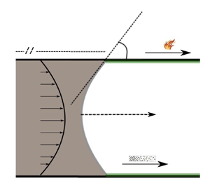
  $({\partial \gamma }/ {\partial z})$. By surfactants here we mean a substance that changes the surface tension of liquids (increase/decrease). Our system that accommodates the aforementioned layouts is depicted in figure 1, showing the interphase portion of a truncated capillary duct.

Figure 1. Representation of axial variation of unsteady surface tension due to spatial longitudinal changes in temperature and surfactant solution lining on the conduit's surface, and contact angle. The velocity profile is depicted distinctively from the interphase.
Through these developments, we note that theory predicts that if surface tension changes across a continuous domain, the imbalance will create motion, forcing the surface to move (see, e.g. Elfring, Leal & Squires Reference Elfring, Leal and Squires2016; Manikantan & Squires Reference Manikantan and Squires2020) characterized by the Marangoni number. Such non-uniformity in surface tension is known to cause bead coalescence cascades (Ji et al. Reference Ji, Falcon, Sedighi, Sadeghpour, Ju and Bertozzi2021). The sum of the shear forces created in both liquids  $(L_{1}\ {\rm and}\ L_{2})$ must exactly equal the gradient of the surface tension,
  ${{\rm \Delta} } \gamma =\tau _{L_{1}}-\tau _{L_{2}}$. According to this, in a viscous fluid the induced velocity
  $u$ is such that
  $u\thicksim {{\rm \Delta} } \gamma / \mu$, where
  ${{\rm \Delta} } \gamma$ represents the difference in surface tension and
  $\mu$ is the average dynamic viscosity of the liquid. The assumption here is that the surface tension is steady and changes are brought to it due to the convective nature of the flow front as it meets regions having different temperatures and surfactant concentrations. Thus, the non-uniformity of the parameter influencing capillarity couples linearly with encroachment speed to modify the interphase configuration through the Gibbs energy and provide a transfiguration in the surface tension. Consequently, we hypothesize that
 \begin{align} \dot{\gamma} \thicksim v_{z}\left(\frac{\partial \gamma}{\partial z} + \frac{\partial \gamma}{\partial T} \frac{\mathrm{d}T}{\mathrm{d}z} \right), \end{align}
where  $v_{z}$ is the encroaching rate.
Studies that have utilized changing surface tension are plenty, but a few cases are worth mentioning. Davis, Liu & Sealy (Reference Davis, Liu and Sealy1974) studied the effect of the surface tension linear gradient inside a circular tube lined with an insoluble surfactant. Meanwhile, Jensen (Reference Jensen1997) extended Davis et al.'s work using a weakly curved circular tube to induce convective motion from inner-to-outer walls of the duct. Other key references include the deformation of a liquid film flowing down an inclined substrate driven by gravity (Kabova, Kuznetsov & Kabov Reference Kabova, Kuznetsov and Kabov2012), a 3-D steady flow of a thin viscous liquid on surfaces having insoluble surfactant by Adler & Sowerby (Reference Adler and Sowerby1970).
Different profiles for temperature and surfactant can be achieved and implemented. However, from a semi-empirical approach the dependence of surface tension with temperature has been modelled as linear for the most part (see, e.g. Navascues Reference Navascues1979; Cassir, Ringuedé & Lair Reference Cassir, Ringuedé and Lair2013; He et al. Reference He, Wylie, Huang and Miura2016). In the absence of a specific temperature gradient and surfactant gradient model represented in figure 1, we recognize the parametric forms
 \begin{align} T(z),\quad \frac{\partial \gamma}{\partial z}(z),\quad v_{z}(t),\quad z(t),\end{align}
and then perform a time integration on (2.4) to obtain a general time-dependent form of  $\gamma (t)$
 \begin{align} \gamma (t)=\gamma_{0} + \gamma_{t}(t), \end{align}
where the surface tension,  $\gamma _{0}$, represents a reference
  $\gamma$ that can be thought of as the initial value of the base liquid. The quantity,
  $v_{z}$, in (2.4) must capture the instantaneous rate of encroachments, thus forcing (2.6) to have a complicated implicit dependence on time. We recognize a common velocity evolution in previous studies,
  $v_{z}\thicksim t^{-1/2}$ (see, e.g. Lucas Reference Lucas1918; Washburn Reference Washburn1921; Fries & Dreyer Reference Fries and Dreyer2008), which is oftentimes valid only for certain conditions (see, e.g. Das et al. Reference Das, Waghmare and Mitra2012; Bhattacharya et al. Reference Bhattacharya, Azese and Singha2017) and even extends to some investigations that involve viscoelastic liquids (Sumanasekara et al. Reference Sumanasekara, Azese and Bhattacharya2017). Ultimately, for this heuristic approach, we avoid lamenting the specific forms in (2.6) and (2.5a–d) and instead surmised a time-monotonic dependence of
  $\gamma (t)$ consequently resulting in the following two forms:
 $$\begin{gather} \mbox{model 1},\quad \gamma (t)=\gamma_{0} (1+r_{\gamma})(1+m{t}), \end{gather}$$
 $$\begin{gather}\mbox{model 2},\quad \gamma (t)=\gamma_{0} ( 1+r_{\gamma}\,{\rm e}^{\xi {t}} ). \end{gather}$$
Here,  $\gamma _{0}\, (\mathrm {N}\,\mathrm {m}^{-1}), r_{\gamma }\,(\mathrm {unitless}), \mathrm {m}\,({\rm s}^{-1})$ and
  $\xi \,(\mathrm {s}^{-1})$ are constant parameters that will be appropriately user-defined to mimic different temporal evolutions. In §§ 4 and 5 transient models (2.7a) and (2.7b) will be used to examine the role of a transitory
  $\gamma (t)$ on capillary imbibition.
3. Description of the flow system and governing equations
The dynamic of the geometry describing our flow system is shown in figure 2. As the  $\gamma$-induced pressure gradient is the only driving force, we consider the system as consisting of two main continuous regions also distinguished by pressure. As shown, these sections are connected through the continuity and momentum balance equation (
 $\widehat {CD}, \widehat {DF}$, with
  $\widehat {EC}$ being the inlet region). This system happens to be similar to that presented in previous papers by one of the authors (Bhattacharya et al. Reference Bhattacharya, Azese and Singha2017; Sumanasekara et al. Reference Sumanasekara, Azese and Bhattacharya2017), and as a result, some details of its descriptions are left out. However, we present a summary in the subsequent paragraphs.

Figure 2. Schematic of the unsteady encroachment of a viscous fluid in an arbitrary capillary conduit driven by the transient surface tension force presented in figure 1. The 1-D flow region is between points  $C$ and
  $D$, meanwhile the 3-D flow follows immediately after. The dynamic pressures are also represented where
  $A, B, C$ are points having an atmospheric pressure similar to the flow from
  $P_{0}$. The pressure gradient driving the 1-D parabolic region, thus responsible for the shape of the parabola, is
  $P_{D}-P_{C}$. Point
  $F$ is in a rigid body translation having a uniform velocity profile.
3.1. Entry region
The flow downstream of the entry region,  $\widehat {EC}$, is dependent on the nature of the surrounding liquid as well as the location and dynamics of the free surface. In applications where hydrostatic pressure is considerable at the inlet, it is typically a 3-D flow. In this configuration some authors have defined a control volume and control surface surrounding the entrance – using these to capture the flow at the conduit inlet (Stange, Dreyer & Rath Reference Stange, Dreyer and Rath2003; Xiao et al. Reference Xiao, Yang and Pitchumani2006; Waghmare & Mitra Reference Waghmare and Mitra2010a; Azese Reference Azese2011). In particular, Azese and Xiao et al. considered a hemispherical control surface to eventually expose the inlet dynamic and obtain an inlet pressure that is dependent on the encroachment rate and the liquid acceleration into the channel.
However, for our system, we simply appraise the entry region as being close to the free surface, thus neglecting strong hydrostatic effects. This leads us to consider the normal flow gradient as non-existent. As a consequence, the inlet flow is uniform and unidirectional (1-D flow), limited by the surface  $ABC$ as shown in figure 2, a consideration also followed in previous papers (Bhattacharya et al. Reference Bhattacharya, Azese and Singha2017; Sumanasekara et al. Reference Sumanasekara, Azese and Bhattacharya2017). We ultimately have
 \begin{align} P_{A} \approx P_{B}\approx P_{C} \thicksim P_{o}= \mbox{atmospheric pressure}. \end{align}
3.2. Core region: unidirectional flow
We describe here the core region of the flow,  $\widehat {CD}$, which is the most important domain hypothesized as a 1-D flow where the detailed flow kinematics and dynamics are developed. Accordingly, this flow region begins just past downstream of the entry region (
 $C$) and ends at the spectral-parabolic front,
  $D$, hence driven by a pressure gradient (
 $P_{C}-P_{D}$). The liquid is assumed to be incompressible; therefore, mass continuity dictates that the lone velocity component,
  $v_{z}$, in the
  $z$ direction be independent of independent variable
  $z$ such that
  ${\boldsymbol {v}}=v_{z}(\boldsymbol {r})\boldsymbol {e}_{z}$. Accordingly, the Navier–Stokes equation is used to evaluate momentum conservation in this region,
 \begin{align} \rho \frac{\partial{v}_{z} }{\partial {t}}= \mu{\nabla}_{{\perp}}^{2} {v}_{z} -\frac{\partial p}{\partial z}, \end{align}
where  $p, t, \rho$ and
  $\mu$ represent pressure, time, fluid density and viscosity, respectively. Meanwhile,
  $\boldsymbol {\nabla }_{\perp }$ is the gradient on planes that are perpendicular to the flow direction.
Because of the axial uniformity of the cross-sectional area and mindful that the liquid is incompressible, a straightforward mass conservation analysis is performed. It reveals that at a given intruded depth,  $h(t)$, the average of the flow velocity on the cross-sectional area (
 $\mathcal {A}$) evaluated at the 1-D flow front is identical to the encroachment rate
 \begin{align} \frac{\mathrm{d} h}{\mathrm{d}t}=\frac{1}{\mathcal{A}}\int {v}_{z} \mathrm{d}\mathcal{A}. \end{align}
Moreover, at any instant of time, the pressure gradient is the same everywhere in the 1-D region so that for the entire region it is related to  $h(t)$ as
 \begin{align} \frac{\partial p}{\partial z}=\frac{P_D(t)-P_C}{h(t)}=\frac{P_{\varDelta}(t)}{h(t)}, \end{align}
where the pressure change  $P_{\varDelta }(t)$ is the time-dependent gauge pressure driving the 1-D flow in this front region shown in figure 2, bearing in mind
  $P_{C} \sim P_{o}$.
To render our system dimensionally flexible, we seek relevant dimensions from the problem and systematically define scales that would be used to make our problem dimension free. We immediately harvest the system's inherent length scale provided by its spanwise dimensions considered earlier as the cross-sectional size,  $l_c$. It can be defined following several combinations of the cross-sectional size discussed in § 6. However, the surface tension-induced pressure gradient in a circular channel of radius
  $R$ having assumed a semi-spherical interphase is
  ${\rm \Delta} P \thicksim 2\gamma /R$, where the surface tension prefactor,
  $2/R$, exactly coincides with the area-to-wetted-perimeter ratio. Motivated by this, we consider the cross-sectional length scale as
 \begin{align} l_c=\frac{{\mathcal{A}}}{\mathcal{P}}, \end{align}
where  $\mathcal {P}$ and
  $\mathcal {A}$ are respectively the perimeter and area of the conduit. As a result of (3.5), the pressure scale is written as
 \begin{align} p_{s}=\frac{\gamma_{o} \mathcal{P}}{\mathcal{A}}. \end{align}
 To obtain the other scales, first, we define  $t_s$,
  $h_s$ and
  $U_{s}$ as scales for time, encroachment depth and velocity, respectively. These together with (3.5) and (3.6) are used in performing a dimensional analysis on (3.2) and (3.3). However, to ensure that all the forces involved are important even in the absence of kinematic changes, we set the coefficients of every force term to unity. The result of these steps is the definition of the remaining three scales. First the time scale,
 \begin{align} t_{s}=\frac{\rho l_{c}^{2}}{\mu}, \end{align}
interpreted as the viscous time scale which is the average time for momentum response transversely across the channel. We note that another time scale can be constructed as $t_{\gamma }=\sqrt {\rho l_{c}^{3}/\gamma _{o}}$, which is important in the dynamics of sedimentation objects and the oscillation of drops and bubbles (Dreyer Reference Dreyer2007). Interestingly, these time scales have been recovered by previous studies (see, e.g. Stange et al. Reference Stange, Dreyer and Rath2003; Das et al. Reference Das, Waghmare and Mitra2012; Das & Mitra Reference Das and Mitra2013; Lu et al. Reference Lu, Wang and Duan2013), where their ratio is used to obtain the dimensionless number, Ohnesorge number (
 $Oh$), a ratio of viscous force to surface tension and inertia forces. Next, the encroachment length and velocity scales are also obtained,
 \begin{align} h_{s}= l_{c}\sqrt{\frac{\rho\gamma_{o} l_{c}}{\mu^{2}}},\quad U_{s}=\sqrt{\frac{\gamma_{o}}{\rho l_{c}}}. \end{align}
To provide a visual perspective of these scales, we evaluate them by using natural physical values typically used in experiments. For this purpose, let us consider a capillary investigation involving water in a capillary tube of an average cross-section length of  $l_{c}=0.15\,\mathrm {mm}$, so that
 \begin{align} \gamma_{o}=0.072\,\mathrm{N}\,\mathrm{m}^{{-}1},\quad \rho=998\,\mathrm{kg}\,\mathrm{m}^{{-}3},\quad \mu=0.001\,\mathrm{Pa}\,\mathrm{s}. \end{align}
With these constant parameters, we obtain
 \begin{align} t_{s}\approx 20\,\mathrm{ms},\quad t_{\gamma}\approx 200\,\mathrm{\mu}{\rm s},\quad h_{s}\approx 15\,\mathrm{mm},\quad U_{s}\approx 0.7\,\mathrm{m}\,\mathrm{s}^{{-}1},\quad p_{s}\approx 0.5\,\mathrm{kN}. \end{align}
Nevertheless, using scales defined in (3.5) to (3.7) and (3.8a,b), the pressure gradient defined in (3.2) and (3.4) is rendered dimension free so that (3.2) and (3.3) now take the non-dimensional forms
 \begin{align} \frac{\partial{\bar{v}_z}}{\partial {\bar{t}}}={\bar{\nabla}_{{\perp}}}^{2} {\bar{v}}_{z} -\frac{\bar{P}_{\varDelta}(t)}{\bar{h}},\quad \frac{\mathrm{d} \bar{h}}{\mathrm{d}\bar{t}}=\int {\bar{v}}_{z} \frac{\mathrm{d}{\mathcal{A}}}{\mathcal{A}}, \end{align}
where the ‘ $\overline {\hspace {0.2cm}}$’ signifies dimensionless such that
  $\bar {v}_z=v_z/U_s$,
  $\bar {t}=t/t_s$,
  $\bar {P}_D=P_D/p_s$,
  $\bar {h}=h/h_s$ and
  $\bar {\boldsymbol {\nabla }}_{\perp }=l_{c}^{2}{\boldsymbol {\nabla }}_{\perp }$ are the dimensionless variables. We note that (3.11a,b) govern capillary flows in conduits of arbitrary but uniform shapes and, thus, will be used in subsequent sections to examine cases for rectangular § 4 and circular § 5 ducts.
3.3. Front region: 3-D flow,  $h_{f}<< h(t)$

Finally, we describe the front region that drives the encroachment which is characterized by a 3-D flow between points  $D$ and
  $F$, as shown in figure 2. Foremostly, we surmise that this region is very thin so that
 \begin{align} h_{f}=o(h(t)). \end{align}
Furthermore, we note that the velocity field in the core 1-D region is spectral parabolic which is the rear end ( $D$) of this front region. Meanwhile, the front end (
 $F$) undergoes a solid body translation and moves like a piston, hence having a uniform profile. To reconcile these two dynamics, we conceive velocity streamlines as diverging towards the walls, thereby swirling owing to the mass conservation. Consequently, the flow between
  $D$ and
  $F$, as seen in figure 2, adopts a convoluted 3-D form. It is worth noting that most scholars do not account for this parabolic-to-unform transition. Nonetheless, implementing (3.5) to (3.7) and (3.8a,b) and enforcing (3.12) reveals the physics that dictates the dynamics of this region. Ultimately, it ensures that the dimensionless Navier–Stokes properly captures the momentum conservation
 \begin{align} \delta\frac{\partial{\bar{\boldsymbol v}}}{\partial \bar{t}}+ \bar{\boldsymbol{v}} \boldsymbol{\cdot} \bar{\boldsymbol{\nabla}} \bar{\boldsymbol{v}}={-} \bar{\boldsymbol{\nabla}} \bar{p} + \delta{\bar{\nabla}^{2}\bar{\boldsymbol{v}}}, \end{align}
where  $\bar {\boldsymbol v}$ and
  $\bar {p}$ are respectively the dimensionless velocity and pressure within this region, and
  $\bar {\boldsymbol {\nabla }}$ is the gradient vector non-dimensionalised with
  $l_c$. In previous research (Bhattacharya et al. Reference Bhattacharya, Azese and Singha2017; Sumanasekara et al. Reference Sumanasekara, Azese and Bhattacharya2017), however, we showed that
  $\delta$ is the effective capillary number defined as
 \begin{align} \delta=\sqrt{\frac{\mu^{2}}{\rho\gamma_{o} l_{c}}}. \end{align}
For instance, using typical parameter values as those suggested in § 3.2, we evaluate  $\delta \sim 0.0096$, and even smaller for a broader range of applications. For this reason,
  $\delta$ can be considered as a small parameter to orchestrate a perturbation analysis on (3.14) where the pressure and velocity fields are expanded,
 \begin{align} \bar{\boldsymbol v}=\sum_{i=0} \delta^{i} \bar{\boldsymbol v}^{(i)},\quad \bar{p}=\sum_{i=0} \delta^{i} \overline{p}^{(i)}. \end{align}
So, provided  $\delta <<1$, the perturbation analysis should proceed such that (3.15a,b) is inserted into (3.13) to procure a hierarchy of equations. Accordingly, the leading-order effect is captured by
 \begin{align} \overline{\boldsymbol{v}}^{\boldsymbol{0}} \boldsymbol{\cdot} \bar{\boldsymbol{\nabla}} \bar{\boldsymbol{v}}^{\boldsymbol{0}} \thicksim - \bar{\boldsymbol{\nabla}} \bar{p}^{0}, \end{align}
which relates to cases with less narrow conduits. Ultimately, the viscous and the unsteady term disappear, and the flow can safely be treated using steady inviscid relations. In such a scenario, which is similar to ours, one can use a control volume analysis averaged over the cross-section. Thus, exploring the Reynolds transport theorem on the steady bounded domain,  $\mathcal {D}$, relates the pressure gradient with the linear momentum fluxes,
 \begin{align} {\rm \Delta} P|_{3D}=1/\mathcal{A} \int_{\mathcal{D}_{\mathcal{A}}}\rho v^{2}\,\mathrm{d}\mathcal{A}. \end{align}
The area integral in (3.17) is calculated over the inlet and outlet ( $D$ and
  $F$) of the domain's boundary,
  $\mathcal {D}_{\mathcal {A}}$, of this front region. Before doing so, we recall that the pressure around the channel inlet (at
  $C$) and outside of the flow front is identified as atmospheric pressure (3.1). Hence, the pressure gradient responsible for the curved profile is gauged as
 \begin{align} P_{D}-{P_{o}}=P_{\varDelta}(t). \end{align}
Furthermore, the pressure at location  $F$ due to surface tension is smaller than
  ${P_{o}}$ so that
 \begin{align} P_{F}-{P_{o}}={-}P_{\gamma}={-}\gamma/l_{c}, \end{align}
leading to
 \begin{align} P_{\gamma}(t)=\frac{\gamma (t) \mathcal{P}}{\mathcal{A}}=p_{s} \bar{\varPhi} (\bar{t}), \end{align}
where  $\bar {\varPhi } (\bar {t})$ is the dimensionless form of (2.7a) and (2.7b) defined as
 \begin{align} \bar{\varPhi} (\bar{t}) =\frac{\gamma (\bar{t})}{\gamma_{o}}. \end{align}
The pressure difference in the 3-D region is obtained by subtracting (3.19) from (3.18). Also, in this zone we recall that velocity goes from a parabolic to a uniform profile. Following these, we eventually evaluate (3.17) in this region to obtain
 \begin{align} \bar{P}_{\varDelta}(\bar{t})+\bar{P}_{\gamma}=\left(\int {\bar{v}}_{z} \left.\frac{\mathrm{d}\mathcal{A}}{\mathcal{A}}\right)^{2}\right|_{{uniform}} -\int {\bar{v}}_{z}^{2} \left.\frac{\mathrm{d}\mathcal{A}}{\mathcal{A}}\right|_{{parabolic}}. \end{align}
Ultimately, we obtain the dictating equations of our problem, governing flow in the 1-D flow region. Thus, by defining  $\mathrm {d}\bar {\mathcal {A}}={\mathrm {d}\mathcal {A}}/{\mathcal {A}}$, we use (3.20) to (3.22) to rewrite (3.2) into its final form for any arbitrary channel, i.e.
 \begin{align} \frac{\partial{\bar{v}_z}}{\partial {\bar{t}}}={\nabla}^{2}_{{\perp}}{\bar{v}}_{z} + \frac{\bar{\varPhi} (\bar{t}) +\int {\bar{v}}_{z}^{2}\,\mathrm{d} \bar{\mathcal{A}}-(\int {\bar{v}}_{z}\,\mathrm{d}\bar{\mathcal{A}})^{2}}{\bar{h}}. \end{align}
Equation (3.23) is a first-order initial boundary value problem having a nonlinear source term, to be solved simultaneously with
 \begin{align} \frac{\mathrm{d} \bar{h}}{\mathrm{d}\bar{t}}=\int_{\partial \mathcal{D}} {\bar{v}}_{z}\,\mathrm{d}\bar{\mathcal{A}}, \end{align}
computed at the parabolic front,  $\partial \mathcal {D}$. In the coming sections both (3.23) and (3.24) are effectively used in examining unsteady imbibition in two well-known channels: conduits having rectangular cross-sectional shapes (§ 4) and those with circular cross-sectional areas (§ 5).
4. Imbibition in a rectangular channel
In this section we analyse the capillary flow due to transient surface tension inside ducts with rectangular cross-sections. This kind of geometric design, frequently encountered in many applications and investigations, presents rich intricacies of its dynamics in laminar flows hidden in its shape, as discussed by Zhang & Xia (Reference Zhang and Xia2007). Many encroachment dynamicists have used rectangular ducts as a platform to further our understanding of capillary action (e.g. Xiao et al. Reference Xiao, Yang and Pitchumani2006; Waghmare & Mitra Reference Waghmare and Mitra2010a) with success – despite inaccurate inherent assumptions or lack of proper physical accountability of the different regions of flow (§§ 3.1–3.3). The flexibility possessed by the robust expression already developed earlier in § 3 in describing unsteady imbibition, is used to observe the fine details exhibited by the rectangular duct.
We begin by considering the channel axis to be at the centre of both boundaries and in the  $z$ direction (figure 2), thus, located at the midway of both walls. Following this, the cross-section of the rectangular conduits is described by prescribing the width,
  $2l_{y}$, and the breadth,
  $2l_{x}$. Here and in the following, we use ‘
 $\ast$’ to differentiate quantities with similar letters or symbols associated with a rectangular duct from those of cylindrical channels. As a consequence, (3.5) becomes
 \begin{align} l_{c}^{{\ast}}=\frac{\mathcal{A}^{{\ast}}}{\mathcal{P}^{{\ast}}}=\frac{l_{x}l_{y}}{l_{x}+l_{y}}. \end{align}
The channel's aspect ratio,  $\kappa$, is defined as
 \begin{align} \kappa=\frac{l_{x}}{l_{y}} \end{align}
so that  $l_{x}$ remains the smallest side, thus ensuring
  $\kappa \le 1$. Using (4.2), we non-dimensionalize the channels half-widths, i.e.
 \begin{align} \overline{l}_{x}=\frac{l_{x}}{l_{c}^{{\ast}}}=\kappa+1,\quad \overline{l}_{y}=\frac{l_{y}}{l_{c}^{{\ast}}}= \frac{\kappa+1}{\kappa}. \end{align}
These results will be crucial in subsequent developments making sure the conduits are properly coupled to the flow solution.
4.1. Unsteady $xy$-eigenfunction expansion

We recall that the flow within the core region of the conduit is predominantly unidirectional. According to this, the dimensionless lone velocity component is defined by
 \begin{align} \boldsymbol{{\bar{v}}^{{\ast}}}=\bar{\boldsymbol v}_{z}^{{\ast}}(\bar{x},\bar{y}, \bar{t}^{{\ast}}){\boldsymbol e}_{z}, \end{align}
whose invariance with  $z$ is dictated by the continuity equation. Considering the spatial variations alone, we recognize that the flow governing differential equation (3.23) is originally a linear type allowing for a spectral expansion of the velocity
 \begin{align} \bar{v}_{z}^{{\ast}}=\sum_i \alpha_{i}^{{\ast}} (\overline{t^{{\ast}}}) u_{i}^{{\ast}}(\bar{x},\bar{y}), \end{align}
where  $i\in \mathbb {N}$ and
  $u_{i}^{\ast }$ are the double-variable eigenfunction and
  $\alpha _{i}^{\ast }$ are the corresponding time-dependent amplitude. Consequently, from Sturm–Liouville's theory one can construct an eigenvalue problem based on the spatial-dependent variables,
 \begin{align} \bar{\nabla}^{{\ast} 2}_{{\perp}} {{u}}_{i}^{{\ast}}={-}\beta^{{\ast} 2}_{i} u_{i}^{{\ast}}, \end{align}
where  $\beta ^{\ast 2}_{i}$ is the eigenvalue of
  $u_{i}^{\ast }$ whose values would be determined by enforcing the proper boundary conditions.
Using (4.5) and (4.6), we take the inner products,  $\langle [(3.23)],u_{j}^{\ast } \rangle$ and
  $\langle [(3.24)],u_{j}^{\ast } \rangle$, of the controlling equations averaged over the cross-sectional area,
  ${\mathcal {\partial A}}$. In the process, we identify and define an important channel geometry-related parameter
  $\eta _{i}^{\ast }$,
 \begin{align} \eta_{i}^{{\ast}}=\int_{\mathcal{\partial A}} u_{i}^{{\ast}} \,\mathrm{d}\overline{\mathcal{A}}^{{\ast}}. \end{align}
In addition, we recognize and enforce the orthogonality requirements such that when normalized we get
 \begin{align}
\int_{\mathcal{\partial A}} u_{i}^{{\ast}}
u_{j}^{{\ast}}\,\mathrm{d}
\overline{\mathcal{A}}^{{\ast}}=\delta_{ij},\quad
\mbox{where}\ \delta_{ij} = \left\{\begin{array}{@{}ll} 0, &
i\neq j, \\ 1, & i=j, \end{array}\right.
\end{align}
\begin{align}
\int_{\mathcal{\partial A}} u_{i}^{{\ast}}
u_{j}^{{\ast}}\,\mathrm{d}
\overline{\mathcal{A}}^{{\ast}}=\delta_{ij},\quad
\mbox{where}\ \delta_{ij} = \left\{\begin{array}{@{}ll} 0, &
i\neq j, \\ 1, & i=j, \end{array}\right.
\end{align}
here  $\delta _{ij}$ is the Kronecker delta. The results of these steps lead to the differential equation governing the unsteady amplitude
 \begin{align} \frac{\mathrm{d} \alpha_{i}^{{\ast}}}{\mathrm{d} \bar{t}}={-}\beta_{i}^{2\ast} \alpha_{i}^{{\ast}}-\eta_{i}^{{\ast}}\frac{\bar{P}^{{\ast}}_{\varDelta}}{\bar{h}^{{\ast}}}. \end{align}
We develop (3.22) to systematically obtain  $\bar {P}^{\ast }_{\varDelta }$. First, recognizing that the front moves as a piston kinematically translates into meaning uniform velocity. Therefore, it is easy to show that
 \begin{align} \left(\int_{\mathcal{\partial A}} {\bar{v}^{{\ast}}}_{z} \mathrm{d}\overline{A}^{{\ast}}\right)^{2} = \left[\sum_{j=1}^{N} \eta_{i}^{{\ast}}\alpha_{i}^{{\ast}}(\bar{t}^{{\ast}})\right]^{2}, \end{align}
where  $N\in \mathbb {N}$ denotes the extent of the velocity spectrum and dictates the accuracy of the summation. Furthermore, at the spectral-parabolic end, Rayleigh's identity is used to manoeuvre between integral and summation, leading to
 \begin{align} \int_{\mathcal{\partial A}} ({\bar{v}}_{z}^{{\ast}})^{2} \mathrm{d}\overline{\mathcal{A}}^{{\ast}} = \sum_{j=1}^{N} (\alpha_{i}^{{\ast}})^{2} (\bar{t}^{{\ast}}). \end{align}
In consequence, we obtain
 \begin{align} \bar{P}^{{\ast}}_{\varDelta}(t)=\left[\sum_{j=1}^{N} \eta_{i}^{{\ast}} \alpha_{i}^{{\ast}}(\bar{t}^{{\ast}})\right]^{2}- \sum_{j=1}^{N} (\alpha_{i}^{{\ast}})^{2} (\bar{t}^{{\ast}}) - \bar{\varPhi}^{{\ast}} (\bar{t}^{{\ast}}). \end{align}
To this end, the governing equations have now been fully separated into spatial and time-dependent parts, owing to the spectral decomposition – yielding forms that will be solved.
4.2. Analytical Fourier solution to rectangular duct
Despite the successful development of the governing equations thus far, their analysis and solutions require that initial and boundary dynamics be reflected in the equations through the independent variables. According to this, first, we recognize an encroachment that begins from the rest, implying that when  $\bar {t}^{\ast }=0, {\bar {v}}_{z}^{\ast } =0$. Moreover, we elect to use the no-slip boundary condition stipulating that flow velocities are identically zero at the four walls. Then, using the argument of the arbitrariness of the free independent variable in the linear homogeneous sums (4.5), we therefore write
 $$\begin{gather} \bar{t}=0,\quad \alpha_{i}^{{\ast}}=0, \end{gather}$$
 $$\begin{gather}\bar{x}={\pm} (\kappa+1),\quad u_{i}^{{\ast}}=0, \end{gather}$$
 $$\begin{gather}\bar{y}={\pm}\left(\frac{\kappa+1}{\kappa}\right),\quad u_{i}^{{\ast}} =0. \end{gather}$$
To this end, we have used one index in denoting  $\alpha _{i}^{\ast }$ and
  $u_{i}^{\ast }$ to indicate the spectrum involved in (4.5), doing so for the sake of generality. However, a closer look at (4.4) and (4.5) reveals that two independent variables are involved, thus requiring rather a bispectral summation,
  $i=n,m$. We solve the Helmholtz equation (4.6) by the method of separation of variables while enforcing the boundary conditions in (4.13b) and (4.13c) to get
 \begin{align} u_{nm}^{{\ast}}=a_{nm}\cos \left(\frac{2n+1}{2}{\rm \pi} \frac{\bar{x}}{\overline{l}_{x}}\right)\cos\left(\frac{2m+1}{2}{\rm \pi} \frac{\bar{y}}{\overline{l}_{y}}\right), \end{align}
where  $a_{mn}$ are constants to be determined. Using the orthogonality relation in (4.8), we obtain
  $a_{nm}=2,\ \forall \ n,m \in \mathbb {N}$, and eventually evaluate
 \begin{align} \beta_{nm}^{{\ast}}=\frac{\rm \pi}{2} \sqrt{\left[ \frac{(2n+1)^{2}}{\overline{l}_{x}^{2}} + \frac{(2m+1)^{2}}{\overline{l}_{y}^{2}}\right ]} = \frac{\rm \pi}{2 (1+\kappa)} \sqrt{[\kappa^{2} (2n+1)^{2} + (2m+1)^{2}]}. \end{align}
Furthermore, using (4.14), the shape parameter in (4.7) is computed as
 \begin{align} \eta_{nm}^{{\ast}}= \frac{8}{{\rm \pi}^{2}} \frac{({-}1)^{n+m}}{(2n+1)(2m+1)}. \end{align}
At this point, what is left is the solution for the unsteady amplitudes governed by
 \begin{align} \frac{\mathrm{d} \alpha_{nm}^{{\ast}}}{\mathrm{d} \bar{t}^{{\ast}}}={-}(\beta_{nm}^{{\ast}})^{2} \alpha_{nm}^{{\ast}}+\frac{\eta_{nm}^{{\ast}}}{\bar{h}^{{\ast}}} \left[\bar{\varPhi}^{{\ast}} (\bar{t}^{{\ast}})+ \sum_{{p=1,q=1}}^{N,M} (\alpha_{pq}^{{\ast}})^{2} (\bar{t}^{{\ast}}) - \left\{\sum_{{p=1,q=1}}^{N,M} \eta_{pq}^{{\ast}}\alpha_{pq}^{{\ast}}(\bar{t}^{{\ast}})\right\}^{2}\right], \end{align}
which is used to evaluate  $\bar {h}^{\ast }$ and
  $\dot {\bar {h}}^{\ast }$ through
 \begin{align} \frac{\mathrm{d}\bar{h}^{{\ast}}}{\mathrm{d}\bar{t}^{{\ast}}} = \sum_{{n=1,m=1}}^{N,M} \eta_{nm}^{{\ast}} \alpha_{nm}^{{\ast}}(\bar{t}^{{\ast}}). \end{align}
Accordingly, (4.17) and (4.18) are evaluated next and used in calculating the kinematics in a rectangular channel to unveil the ins and outs of this transient  $\gamma (t)$ puzzle.
4.3. Results and discussion of capillarity in a rectangular channel
4.3.1. Preliminaries: rectangular data
To appreciate the unsteady effects of surface tension in a confined rectangular conduit, we perform a numerical evaluation of (4.17) and (4.18). To do so, first, we identify (4.18) as a first-order initial value (IV) problem – characterized by an ODE – with a source term,  $f_{\bar {h}^{\ast }}$, recognized as a convoluted function
 \begin{align} f_{\bar{h}^{{\ast}}}=f_{\bar{h}^{{\ast}}} \left(\alpha_{nm}^{{\ast}}(\bar{t}^{{\ast}},\bar{h}^{{\ast}}(\bar{t}^{{\ast}} ))\right), \end{align}
thus having two dependent arguments. Next, we also recognize the ODE in (4.17) as another first-order, inhomogeneous IV problem with a convoluted nonlinear source term represented by the function  $f_{\alpha ^{\ast }}$ such that
 \begin{align} f_{\alpha^{{\ast}}}= f_{\alpha^{{\ast}}} \left( \bar{h}^{{\ast}}(\bar{t}^{{\ast}}), \alpha_{nm}^{{\ast}}(\bar{t}^{{\ast}}, \bar{h}^{{\ast}}(\bar{t}^{{\ast}} )), (\bar{t}^{{\ast}}) \right). \end{align}
Hence, an analytical solution does not exist for (4.17). In addition, we also take note of the obvious singularity for  $\bar {h}^{\ast }=0$. Fortunately, our system is intended to allow for a non-zero a priori filled depth. Ultimately, we recommend
 \begin{align} \mbox{at} \quad \bar{t}^{{\ast}}=0,\quad \bar{h}^{{\ast}}_{0} \ne 0,\quad \bar{h}^{{\ast}}_{0} \lesssim \bar{\mathcal{J}}_{{h}}^{{\ast}},\quad \bar{\mathcal{J}}_{{h}}^{{\ast}} \sim \sqrt{\gamma_{o}/(\rho g l_{c}^{{\ast}} h_{s}^{{\ast}})}, \end{align}
where  $\bar {\mathcal {J}}_{{h}}^{\ast }$ is the equivalent of Jurin's height for vertical narrow rectangular conduits based on the steady surface tension. This is so because we expect the penetrating flow to have more momentum and, consequently, more penetrated depth due to the absence of a slowing-down force of gravity and the presence of surface tension accelerants.
4.3.2. Numerical scheme
Here we describe the numerical algorithm used in completing solutions that describe unsteady capillary flow in rectangular channels. We note that the algorithm developed here will also be used to compute data for cylindrical channels in § 5. We begin by recalling that (4.17) and (4.18) are both IV problems describing the spectral amplitudes and encroachment depth feeding values to each other at every instance of time – showcasing a strong dependence between them – with nonlinear source terms. Therefore, because they are coupled, we use a Runge–Kutta fourth-order scheme simultaneously, which avoids implementing a numerical integration scheme since  $\bar {h}^{\ast }$ depends on the spectrum and history of
  $\alpha _{i}^{\ast }$. Accordingly, the discretized source terms (4.19) and (4.20) feed on both of their previously calculated values.
A convergence analysis is done to obtain proper iteration time steps  $({\rm \Delta} \bar {t}^{\ast })$ and mesh sizes
  $({\rm \Delta} \bar {x}^{\ast },{\rm \Delta} \bar {y}^{\ast })$. According to our numerical validation tests, we settled on
  ${\rm \Delta} \bar {t}^{\ast }=0.0001$ while truncating the spectrum to
  $N=40$ and
  $M=40$ having a maximum numerical local error of
  $<0.001\,\%$ compared with
  ${\rm \Delta} \bar {t}^{\ast }=0.01, N=20$ and
  $M=20$. Moreover, it ensures that the relative error due to the spectral convergence is
  $<0.01\,\%$ . It is interesting to note that the magnitude of these incremental steps excellently resolves all the micro-details of the flow also informed by the exponential time growths,
  $\overline {\xi }^{\ast }$, and linear-time gradients,
  $\bar {m}^{\ast }$. Ultimately, the outputs of these simulations are the time history of encroachment,
  $\bar {h}^{\ast }$, and their corresponding encroachment rate
  $\dot {\bar {h}}^{\ast }$, thus at every time step
  $\bar {t}^{\ast }$.
4.3.3. Data and results: rectangular duct
For the present case of a rectangular duct, the simulations are done using the following two transient models for surface tension:
 $$\begin{gather} \mbox{model 1},\quad \bar{\varPhi}^{{\ast}} (\bar{t}^{{\ast}})=(1+r_{\gamma})(1+\bar{m}^{{\ast}} \bar{t}^{{\ast}}), \end{gather}$$
 $$\begin{gather}\mbox{model 2},\quad \bar{\varPhi}^{{\ast}} (\bar{t}^{{\ast}})=1+r_{\gamma} \exp({\overline{\xi}^{{\ast}} \bar{t}^{{\ast}}}). \end{gather}$$
Here  $r_{\gamma }^{\ast }$,
  $\bar {m}^{\ast }$ and
  $\overline {\xi }^{\ast }$ are free parameters, thus user-prescribed. Furthermore, for this channel, we will evaluate and examine cases for three aspect ratios: square channels
  $\kappa =1$, double square
  $\kappa =0.5$ and slit pore
  $\kappa \approx 0.01$.
It is worth mentioning that inertia effects are best captured using small values of prefilled depth. We successfully tested small-scale values using  $\bar {h}^{\ast }_{0}\thicksim 0.001$ and
  $\bar {h}^{\ast }_{0}\thicksim 0.01$, although we elected not to present the data. Nonetheless, a compelling observation was made. At early times the rate of change of encroachment velocity (
 $\mathrm {d}\bar {v}^{\ast }/\mathrm {d}\bar {t}^{\ast }$) was relatively high for minuscule
  $\bar {h}^{\ast }_{0}$ – this is also dictated by the last term in (4.9) – it initially blows up the inertia effects. Consequently, it required correspondingly small time intervals (
 ${{\rm \Delta} } \bar {t}^{\ast }$) to highlight the details at early times. So, using (3.9a–c) and (3.10a–e), the equivalent Jurin's depth is estimated from (4.21) as
  $\bar {\mathcal {J}}_{{h}}^{\ast }\thicksim 1.8$. However, for both conduits, we chose to present only cases having pipetted depth ranging from
  $\bar {h}^{\ast }_{0}=0.2$ to
  $\bar {h}^{\ast }_{0}=5$, considered here as a moderate-to-high range, allowing us to also examine the effects of initial over filled. Worthy of note is that our choices within this range are also motivated by those used in Bhattacharya et al. (Reference Bhattacharya, Azese and Singha2017) and Sumanasekara et al. (Reference Sumanasekara, Azese and Bhattacharya2017). Using typical experimental values described in § 3.2 this range corresponds to
  ${h}^{\ast }_{0} \thicksim 3\,\mathrm {mm}-{h}^{\ast }_{0} \thicksim 70\,\mathrm {mm}$.
Furthermore, we caution that, except for figures 13 and 14, graphs with expressions involving penetrated depth  $f(\bar {h})$ and correspondingly those having to do with encroachment rates
  $f(\bar {v})$ will be plotted side-by-side. Accordingly, for each set of data,
  $f(\bar {h})$ will be plotted on the right axes whereas
  $f(\bar {v})$ will be plotted on the left axes.
The data for this conduit are presented in a total of three figures. Accordingly, cases for  $\gamma$-model 1 (4.22a) are presented in figure 3, whereas those for
  $\gamma$-model 2 (4.22b) are depicted in figures 4 and 5. More to this, in figures 3 and 5, the choices of parameters ensure a monotonic and an increasing
  $\gamma (t)$. Meanwhile, cases with rather monotonic-and-decreasing time-dependent surface tensions are plotted in figure 4. To appreciate the importance of unsteadiness in surface tension, we have included corresponding plots for steady surface tension represented by the solid black lines. Nonetheless, the plots shown here are quite distinct from each other corresponding to different surface tension modes that reflect the trend and monotonicity of the
  $\gamma$ models. It can also be observed that the encroachment depths show a monotonic increase supported by the fact that the encroachment rates stay positive throughout. Meanwhile, encroachment rates initially increase rapidly reaching maximum values of
  $\bar {v}^{\ast }_{max}$ and then adopting a monotonic decrease. This maximum can be explained by the dynamics involved in that despite the changing capillary force (
 $F_{\gamma }^{\ast }$), the viscous resistance term
  $F_{\mu }^{\ast }$ develops quickly and tones down the growth of the encroachment rate. Additionally, we should recall that
  $F_{\mu }^{\ast }$ is locally weighted by the inverse of encroachment depth that dampers the flow. Consequently, when
  $F_{\mu }^{\ast }$ exactly matches
  $F_{\gamma }^{\ast }$, this growth is expected to stop.

Figure 3. Plots for encroachment rate,  $\bar {v}^{\ast }$ (left axes and thicker lines), and corresponding depth,
  $\bar {h}^{\ast }$ (right axes and corresponding thinner lines), for a channel with a rectangular cross-section given by (4.17) and (4.18) using the unsteady linear-time
  $\gamma (t)$ model in (4.22a). Cases for different prefilled depths are represented where (a,b)
  $\bar {h}_{0}^{\ast }=0.2$ and (c,d)
  $\bar {h}_{0}^{\ast }=5$. The plots also show the kinematics for two different aspect ratios: (a,c)
  $\kappa =1$ and (b,d)
  $\kappa =0.01$. The parameter
  $r_{\gamma }=0, 0.2, 0.5$ and 0.8 corresponding to different
  $m^{\ast }=0, 0.01, 0.05$ and 0.1. Stable
  $\gamma (t)$ are shown with solid-black lines to contrast the dynamics in the transient case.


It is interesting to note the rapport of the intricate features depicted by these plots with previous similar studies for cases of uniform  $\gamma$ (e.g. Lu et al. Reference Lu, Wang and Duan2013; Sumanasekara et al. Reference Sumanasekara, Azese and Bhattacharya2017). For example, the rise and fall of the encroachment rates and having trends whose magnitudes increase with an increasing
  $\gamma$. Not surprising that the comparability is stronger for cases of moderately transient surface tension and smaller initially filled depth, which corresponds to the specific graphs in figures 3–5(a,b).
Additionally, long-time trends of  $\bar {h}^{\ast }$ and
  $\bar {v}^{\ast }$ have characteristics of asymptotic behaviour and § 7 will be dedicated to analytically capturing these exploits. Moreover, the monotonic decreasing version of
  $\gamma$-model 2 generates cases that saturate at a constant value for the long-time run also identified for cases of steady
  $\gamma$ – this will also be examined in § 7. Another important observation is that prefilling the conduit with more liquids (considerable values of
  $\bar {h}^{\ast }_{0}$) causes the velocity to grow in a more strictly increasing trend. This is more prevalent in the faster-growing
  $\gamma$ model (figures 3(c,d), 4(c,d) and 5(c,d)). Perhaps because the strength of the growth rate undermines the decelerating contribution of the inverse of the encroached depth. Finally, a quick comment on aspect ratio, we also note that, in general, square channels have a faster growth rate in
  $\dot {\bar {h}}^{\ast }$ and, for the cases where
  $\bar {h}^{\ast }_{max}$ exist, a correspondingly slower decay rate after it reaches maximum.
5. Imbibition in circular channel
Here we showcase our analysis by considering a confined conduit having a circular cross-section, taking advantage of the flexibility in the governing equations. Small-scale cylindrical-shaped conduits are more practical ducts; for instance, naturally occurring small-flow devices like blood vessels and xylem ducts or applications requiring small channels like medical needles and syringes. It has been used in the past to study capillary action also (see, e.g. Davis et al. Reference Davis, Liu and Sealy1974; Ichikawa & Satoda Reference Ichikawa and Satoda1993; Fries & Dreyer Reference Fries and Dreyer2008; Baek et al. Reference Baek, Jeong, Seo, Lee, Park, Choi, Jeong and Sung2021). However, there are some similarities with its rectangular counterpart in § 4 that we make several references to. So, to differentiate from the previous conduit case, we use ‘ ${\dagger}$’ to refer to quantities that are strictly tied with a circular duct.
We recall that the flow inside the channel is predominantly unidirectional, having axisymmetry, thus, invariant in rotation angle. Hence, leaving the radius as the only spatial independent coordinate. Thus, in dimensionless form, we can write
 \begin{align} {\bar{\boldsymbol v}}^{{{\dagger}}}=\bar{v}_{z}^{{{\dagger}}}(\bar{r} , \bar{t}^{{{\dagger}}}){\boldsymbol e}_{z}. \end{align}
Taking  $r_{o}$ as the radius of the channel, the cross-sectional length scale in (3.5) becomes
 \begin{align} l_c^{{{\dagger}}}=\frac{\mathcal{A}^{{{\dagger}}}}{\mathcal{P}^{{{\dagger}}}}= \frac{r_{o}}{2} \end{align}
and the pressure scale yields
 \begin{align} p_{s}^{{{\dagger}}}=\frac{\gamma_{o} \mathcal{P}^{{{\dagger}}}}{\mathcal{A}^{{{\dagger}}}}=\frac{2\gamma_{o}}{r_{o}}. \end{align}
Using (5.2), the time, axial displacement and velocity scales are restated from (3.7) and (3.8a,b) and redefined as
 \begin{align} t_{s}^{{{\dagger}}}=\frac{\rho (l_{c}^{{{\dagger}}})^{2}}{\mu}=\frac{\rho r_{o}^{2}}{4\mu},\quad h_{s}^{{{\dagger}}}= l_{c}^{{{\dagger}}}\sqrt{\frac{\rho\gamma_{o} l_{c}^{{{\dagger}}}}{\mu^{2}}}= r_{o} \sqrt{\frac{\rho\gamma_{o} r_{o}}{8\mu^{2}}},\quad U_{s}^{{{\dagger}}}=\sqrt{\frac{\gamma_{o}}{\rho l_{c}^{{{\dagger}}}}}=\sqrt{\frac{2\gamma_{o}}{\rho r_{o}}}.\end{align}
With these new scales, the governing equations become
 \begin{align} \frac{\partial{ \bar{v}_z^{{{\dagger}}}}}{\partial {\bar{t}^{{{\dagger}}}}}= (\bar{\nabla}_{{\perp}}^{{{\dagger}}})^{2} {\bar{v}}_{z}^{{{\dagger}}} -\frac{\bar{P}^{{{\dagger}}}_{\varDelta}}{\bar{h}^{{{\dagger}}}},\quad \frac{\mathrm{d} \bar{h}^{{{\dagger}}}}{\mathrm{d}\bar{t}^{{{\dagger}}}}= \int_{\partial \mathcal{D}}{\bar{v}}_{z}^{{{\dagger}}}\,\mathrm{d}\overline{\mathcal{A}}^{{{\dagger}}}. \end{align}
Due to the angular invariance of the flow, the area integral over the circular cross-section,  $\partial \mathcal {D}$, which is already summed over the angular coordinate, is henceforth reduced to only a single radial integral such that
 \begin{align} \mathrm{d}\overline{\mathcal{A}}^{{{\dagger}}}=2r\,\mathrm{d} r/r_{o}^{2}=\bar{r}\,\mathrm{d}\bar{r}/2. \end{align}
Similar to the rectangular case, we use the  $\gamma$ models rescaled as
 $$\begin{gather} \mbox{model 1},\quad \bar{\varPhi}^{{{\dagger}}} (\bar{t}^{{{\dagger}}})=(1+r_{\gamma})(1+\bar{m}^{{{\dagger}}} \bar{t}^{{{\dagger}}}), \end{gather}$$
 $$\begin{gather}\mbox{model 2},\quad \bar{\varPhi}^{{{\dagger}}} (\bar{t}^{{{\dagger}}})=1+r_{\gamma} \exp({\overline{\xi}^{{{\dagger}}} \bar{t}^{{{\dagger}}}}). \end{gather}$$
5.1. Unsteady $r$-polar eigenfunction expansion

A close examination of the governing partial differential equation and ODE, given by (5.5a,b) reveals that it is also suitable for a Sturm–Liouville-type eigenfunction expansion, similar to our observations in § 4.1. According to this, if we consider and redefine the radial dependent eigenfunction as  $u_{i}^{{\dagger} }=\mathscr {R}_{i}(\bar {r})$, the scalar component of (5.1) is expressed in its spectral form as
 \begin{align} \bar{v}_{z}^{{{\dagger}}}=\sum_i \alpha_{i}^{{{\dagger}}} (\bar{t}^{{{\dagger}}}) \mathscr{R}_{i}(\bar{r}), \end{align}
where we remind the reader that  $\bar {r}=r/l_{c}^{{\dagger} }$ and
  $\alpha _{i}^{{\dagger} }$ are the unsteady polar amplitudes. As the first step, we substitute (5.8) into (5.5a,b) and then analyse the inner products,
  $\langle [(5.5\textit{a,b})], \mathscr {R}_{j} \rangle$, over the cross-section. We also identify the Helmholtz eigenfunction equation similar in its compact form as (4.6) given by
 \begin{align} {\bar{\nabla}_{{\perp}}^{{{\dagger}} 2}} {\mathscr{R}}_{i}={-}{{\beta_{i}}^{{{\dagger}}}}^{2} \mathscr{R}_{i}. \end{align}
Along the process, a surface parameter is also recognised and defined as
 \begin{align} \eta_{i}^{{{\dagger}}}=\int_{\partial \mathcal{D}} \mathscr{R}_{i}\,\mathrm{d}\overline{\mathcal{A}}^{{{\dagger}}}, \end{align}
where the nature of the equations imposes an orthogonality condition
 \begin{align} \int_{\partial \mathcal{D}} \mathscr{R}_{i} \mathscr{R}_{j}\,\mathrm{d}\overline{\mathcal{A}}^{{{\dagger}}}=\delta_{ij}. \end{align}
Here also,  $\delta _{ij}$ is the Kronecker delta interpreted in the same way as (4.8). The outcome of these steps leads to a first-order ODE governing the unsteady amplitude
 \begin{align} \frac{\mathrm{d} \alpha_{i}^{{{\dagger}}}}{\mathrm{d} \bar{t}^{{{\dagger}}}}={-}{{\beta_{i}}^{{{\dagger}}}}^{2} \alpha_{i}-{\eta}_{i}^{{{\dagger}}} \frac{\bar{P}^{{{\dagger}}}_{\varDelta}}{\bar{h}^{{{\dagger}}}}. \end{align}
We focus next on developing (3.22) to obtain the driving pressure difference. Again from Parseval's theorem, we use (5.8) and (5.10) to analyse the momentum flux at the spectral-parabolic flow front to systematically show that
 \begin{align} \left(\int_{\partial \mathcal{D}} \bar{v}_{z}^{{{\dagger}}}\,\mathrm{d}{\overline{\mathcal{A}}^{{{\dagger}}}}\right)^{2} = \left[\sum_{i=1}^{N} \eta_{i}^{{{\dagger}}} \alpha_{i}^{{{\dagger}}}({\bar{t}^{{{\dagger}}}})\right]^{2}. \end{align}
Meanwhile, at the free surface where the velocity is uniform, we easily show that
 \begin{align} \int_{\partial \mathcal{D}} {\bar{v}_{z}^{{{\dagger}} 2}}\,\mathrm{d}{\overline{\mathcal{A}}^{{{\dagger}}}} = \sum_{i=1}^{N} {\alpha_{i}^{{{\dagger}}}}^{2} ({\bar{t}^{{{\dagger}}}}). \end{align}
The final expression from the aforementioned steps is therefore
 \begin{align} \bar{P}^{{{\dagger}}}_{\varDelta}= \left\{\left[\sum_{i=1}^{N} \eta_{i}^{{{\dagger}}} \alpha_{i}^{{{\dagger}}}({\bar{t}^{{{\dagger}}}})\right]^{2}- \sum_{i=1}^{N} {\alpha_{i}^{{{\dagger}}}}^{2} ({t^{{{\dagger}}}}) -\bar{\varPhi}^{{{\dagger}}} (\bar{t}^{{{\dagger}}})\right\}, \end{align}
leading to a final set of governing ODE,
 $$\begin{gather} \frac{\mathrm{d} \alpha_{i}^{{{\dagger}}}}{\mathrm{d} \bar{t}^{{{\dagger}}}}={-}{{\beta_{i}}^{{{\dagger}}}}^{2} \alpha_{i}^{{{\dagger}}}-{\eta}_{i}^{{{\dagger}}}\left\{\left[\sum_{j=1}^{N} \eta_{j}^{{{\dagger}}} \alpha_{j}^{{{\dagger}}}({\bar{t}^{{{\dagger}}}})\right]^{2}- \sum_{j=1}^{N} {\alpha_{j}^{{{\dagger}}}}^{2} ({t^{{{\dagger}}}}) -\bar{\varPhi}^{{{\dagger}}} (\bar{t}^{{{\dagger}}}) \right\}, \end{gather}$$
 $$\begin{gather}\frac{\mathrm{d} \bar{h}^{{{\dagger}}}}{\mathrm{d}\bar{t}^{{{\dagger}}}}=\sum_{i=1}^{N} \eta_{i}^{{{\dagger}}} \alpha_{i}^{{{\dagger}}}. \end{gather}$$
5.2. Analytical Bessels solution for a circular channel
We provide a detailed analysis leading to a solution for the eigenfunctions describing the velocity profile. First, for solution closure, we define the two boundary conditions
 $$\begin{gather} \bar{r}=0,\quad \mathscr{R}_{i}= \mbox{sup} (\mathscr{R}_{i}) \implies \frac{\mathrm{d} \mathscr{R}_{i}}{\mathrm{d}\bar{r}}=0, \end{gather}$$
 $$\begin{gather}\bar{r}=2,\quad \mathscr{R}_{i}=0,\quad \mbox{no-slip}, \end{gather}$$
where (5.17a) is due to the angular symmetry requiring the maximum flow speed occurring at the centre. Meanwhile, (5.17b) enforces that the fluid sticks to the stationary wall. Next, we expand the Laplacian operator in cylindrical coordinates – minding angular symmetry while retaining only the radial components. As a result, (5.9) takes the form
 \begin{align} \bar{r}^{2} \frac{\mathrm{d}^{2} {\mathscr{R}}_{i}}{\mathrm{d}\bar{r}^{2}} + \bar{r}\frac{\mathrm{d} {\mathscr{R}}_{i}}{\mathrm{d}\bar{r}}+\bar{r}^{2} {{\beta_{i}}^{{{\dagger}}}}^{2} \mathscr{R}_{i}=0, \end{align}
recognized here as the classical Bessel's ODE. It is a linear second-order differential equation suggesting two independent solutions. According to Bessel's analysis, the general solution is given by
 \begin{align} \mathscr{R}_{i}=c_{1} {J_{0}}({\beta}_{i}^{{{\dagger}}} \bar{r})+c_{2} Y_{0} ({\beta}_{i}^{{{\dagger}}} \bar{r}), \end{align}
where  $c_{1}$ and
  $c_{2}$ are constants, whereas
  ${J_{0}}$ and
  $Y_{0}$ are zeroth-order Bessel functions of the first and second kind, respectively. These two functions can be written in terms of power series, which reveals that
  $Y_{0}({\beta }_{i}^{{\dagger} } \bar {r})$ admits a singularity at
  $\bar {r}=0$. In what follows, we would make use of two integral identities of Bessel's functions,
 \begin{align} \int_{0}^{2} {J_{0}}({\beta}_{i}^{{{\dagger}}} \bar{r}) \bar{r}\,\mathrm{d} \bar{r}= 2\frac{{J_{1}}(2{\beta}_{i}^{{{\dagger}}})}{{\beta}_{i}^{{{\dagger}}}},\quad \int_{0}^{2} {J_{0}}^{2}({\beta}_{i}^{{{\dagger}}} \bar{r}) \bar{r}\,\mathrm{d} \bar{r}= 2[{{J_{0}}^{2}(2{\beta}_{i}^{{{\dagger}}})} + {J_{1}^{2} (2{\beta}_{i}^{{{\dagger}}})}]. \end{align}
We enforce the boundary conditions in (5.17) while implementing the orthogonality condition in (5.11) and making use of (5.20a,b). In the end, solutions for the spectral polar eigenfunctions are secured,
 \begin{align} \mathscr{R}_{i} = \frac{{J_{0}}({\beta}_{i}^{{{\dagger}}} \bar{r})}{{J_{1}}(2\beta_{i}^{{{\dagger}}})}. \end{align}
Through this development, (5.17b) informs that the eigenvalues of the Helmholtz equation,  ${\beta }_{i}^{{\dagger} }$, be obtained by finding the roots of
 \begin{align} {{J_{0}}(2{\beta}_{i}^{{{\dagger}}} )} =0. \end{align}
Using (5.20a,b), the shape flow factor for this circular conduit defined in (5.10) is also computed,
 \begin{align} {\eta}_{i}^{{{\dagger}}} =\frac{1}{\beta_{i}^{{{\dagger}}}}. \end{align}
Ultimately, the final version of the ODE dictating the transient amplitude outlined
 \begin{align} \frac{\mathrm{d} \alpha_{i}^{{{\dagger}}}}{\mathrm{d} {\bar{t}^{{{\dagger}}}}}={-}{\beta_{i}^{{{\dagger}}}}^{2} \alpha_{i}^{{{\dagger}}}- \frac{{\eta}_{i}^{{{\dagger}}}}{{\bar{h}^{{{\dagger}}}}} \left\{\left[\sum_{j=1}^{N} \eta_{j}^{{{\dagger}}} \alpha_{j}^{{{\dagger}}}({\bar{t}^{{{\dagger}}}})\right]^{2}- \sum_{j=1}^{N} {\alpha_{j}^{{{\dagger}}}}^{2} ({\bar{t}^{{{\dagger}}}}) -\bar{\varPhi}^{{{\dagger}}} (\bar{t}^{{{\dagger}}}) \right\} \end{align}
and
 \begin{align} \bar{v}_{z}^{{{\dagger}}}= \frac{\mathrm{d} \bar{h}^{{{\dagger}}}}{\mathrm{d} {\bar{t}^{{{\dagger}}}}}= \sum_{i=1}^{N} \eta_{i}^{{{\dagger}}} \alpha_{i}^{{{\dagger}}} (\bar{t}^{{{\dagger}}}) = \sum_{i=1}^{N} \frac{ \alpha_{i}^{{{\dagger}}}}{ \beta_{i}^{{{\dagger}}} } \end{align}
for  $i=1,2,\ldots,N$.
5.3. Numerical scheme, results and comments: circular channel
The two resulting governing ODEs (5.24) and (5.25) are indeed first order. Besides being a single-spectral summation, they are identical in form to (4.17) and (4.18) in § 4. Moreover, we also note the similarities existing in their non-trivial source terms (4.19) and (4.20), thus warranting an identical computational treatment. As a result, (5.24) and (5.25) are tackled simultaneously using the same numerical scheme described in § 4.3.2. Thus, we evaluate them numerically, calculating the relevant kinematics data:  $\bar {h}^{{\dagger} }$ and
  $\bar {v}^{{\dagger} }$.
The ODEs (5.24) and (5.25) are solved using the rescaled unsteady  $\gamma$ models in (5.7).
According to § 4.3.2, a fourth-order Runge–Kutta algorithm is used to simultaneously solve the two ODEs for different unsteady  $\gamma$ using a different set of parameters (
 $r_{\gamma }^{{\dagger} }$,
  $m^{{\dagger} }$ and
  $\xi ^{{\dagger} }$) for two values of initially filled depth:
  $\bar {h}_{o}^{{\dagger} }=0.2$ and 5.
These data are presented in figure 6 for  $\gamma$-model 1 and figures 7 and 8 for
  $\gamma$-model 2. Qualitatively, their kinematics and dynamics resemble those of the rectangular conduit. This can be seen in the identical calculus features of their respective governing equations, also discussed in § 4.3.3. For the presented parameters, this quantitative time similarity is evaluated at
  ${\gg }80\,\%$ (see § 6). Because of this, we omit the detailed qualitative interpretation, deferring to that outlined in § 4.3.3 about their rectangular counterparts. We determine later in § 6 that the similarities in quality and quantity are better when the rectangular channel has a square (
 $\kappa =1$) or a square-doubled (
 $\kappa =0.5$) shape.


6. Contrasting creeping rates for both channels
Thus far, two channels with different cross-sectional shapes have been analysed to uncover the effects of unsteadiness of transient surface tensions in capillary encroachment. Each of these configurations is important for different applications. In the previous sections, particularly § 5.3, some similarities were noted, which motivated a closer look. It is well established that the size and shape of flow conduits strongly influence the dynamics involved in narrow channel hydrodynamics (see, e.g. Akbari, Sinton & Bahrami Reference Akbari, Sinton and Bahrami2011; Navardi, Bhattacharya & Azese Reference Navardi, Bhattacharya and Azese2016). Many combinations of dimensions that are related to the cross-sectional shape have been used in constructing relevant transverse length scales (Bahrami, Michael Yovanovich & Richard Culham Reference Bahrami, Michael Yovanovich and Richard Culham2007; Moharana & Khandekar Reference Moharana and Khandekar2013; Akbari et al. Reference Akbari, Sinton and Bahrami2011). These include the hydraulic radius and the square root of the area. However, from the onset, we differed from the aforementioned definitions. We are reminded of our definition for transverse breath scales  $l_{c}$, as the ratio of area-to-perimeter, a variant to the other pertinent scales (3.5)–(3.8a,b) and (3.7).
Ultimately, the three forces in action within our system,  $F_v$,
  $F_\mu$ and
  $F_\gamma$, are substantially affected by these gauges. Interestingly, an important connection can be made between the dictating scales (3.5)–(3.7) and (3.8a,b). This observation stipulates that if the fluids’ properties (
 $\rho,\mu,\ {\rm and}\ \gamma _{o}$) are held fixed, then the invariance of
  $l_{c}$ ensures identical scales between two conduits of arbitrary shapes. Therefore, for two different channels having alike length scales, there exist an infinite number of ways of combining the remaining unconstrained parameters (
 $\rho,\mu$ and
  $\gamma _{o}$). This ambiguity therefore needs to be approached carefully while juxtaposing the two shapes.
Foremostly, if  $\mathscr {A}$ and
  $\mathscr {P}$ represent the cross-sectional area and perimeter of an arbitrary conduit then, for two arbitrary shaped channels, we can define
 \begin{align} \mathscr{A}_{r}=\frac{\mathscr{A}^{{{\dagger}}}}{\mathscr{A}^{{\ast}}},\quad \mathscr{P}_{r}=\frac{\mathscr{P}^{{{\dagger}}}}{\mathscr{P}^{{\ast}}}, \end{align}
where the subscript  $r$ refers to ratios such that (6.1a,b) respectively define the quotients between cross-sectional areas and perimeters. A consequence of (6.1a,b) is that if the channels considered are circular and rectangular conduits, then it also follows that
 $$\begin{gather} r_{o}=2 \left(\frac{\mathscr{A}_{r}}{\kappa {\rm \pi}}\right)^{1/2}l_{x}, \end{gather}$$
 $$\begin{gather}r_{o}=2 \left(\frac{1+\kappa}{\kappa {\rm \pi}} \mathscr{P}_{r}\right)l_{x}. \end{gather}$$
Furthermore, for rectangular and circular conduits, it is fortunate that their perimeters have straightforward correlations with their respective cross-sectional area, i.e.
 \begin{align} \mathscr{P}^{{\ast}}/\mathscr{A}^{{\ast}}=2/r_{o},\quad \mathscr{P}^{{{\dagger}}}/\mathscr{A}^{{{\dagger}}}=(1+\kappa)/l_{x}, \end{align}
which we subsequently explore – sadly this is not the case for all arbitrary shape channels. Worth restating is that the magnitudes of  $\mathscr {A}$ and
  $\mathscr {P}$ both play important roles in characterizing the relevant forces involved in capillary encroachment. Following that, the perimeter affects the magnitude of the viscous drag force and capillary force, whereas the area influences the size of the inertia force. Based on the matching parameter of interest, (6.2a) and (6.2b) can be used to provide the correspondences between channel radius and conduit cross-sectional lengths. We are keeping aside other geometric and dynamic intricacies hidden in the shapes that may couple with the flow physics and manifest during capillary imbibition. So, besides the complexity of comparing the display of the convoluted dynamics within the channel, matching the respective (i) length scales,
  $l_{c}^{\ast }\equiv l_{c}^{{\dagger} }$; (ii) cross-sectional area,
  $\mathscr {A}^{\ast }\equiv \mathscr {A}^{{\dagger} }$ and (iii)
  $\mathscr {P}^{\ast }\equiv \mathscr {P}^{{\dagger} }$, is near impossible.
However, in this comparative investigation we chose to ensure that the length scales are similar, consequently fixing corresponding gauges in (3.5)–(3.8a,b) and (3.7). This will enable us to compare the dynamics and kinematics in both channels by having their graphs superposed on each other without prefactors. Ideally, from (6.1a,b), we want both ratios to be unity. However, it is intuitive to examine the similarities existing between a square channel of half-length  $l_{x}$ and a tube such that
 \begin{align} r_{o}=l_{x}. \end{align}
This scenario can be achieved first by taking  $\kappa =1$, and then by making both ratios in (6.1a,b) equal but sadly not unity, such that we now have
 \begin{align} \mathscr{A}_{r}=\mathscr{P}_{r}=\kappa {\rm \pi}/4. \end{align}
Hence, to enforce (6.4) and compare both channels, we keep in mind the presence of the mismatch in (6.5), which eventually influences and differentiates their respective dynamics. Ultimately, the search for a proper match between both channels results in an optimization problem involving the areas, perimeters and length scales. Dividing (6.2a) and (6.2b) results in a quadratic equation in  $\kappa$,
 \begin{align} \mathscr{P}_{r}^{2} \kappa^{2}+ (2 \mathscr{P}_{r}^{2}-{\rm \pi} \mathscr{A}_{r}) \kappa + \mathscr{P}_{r}^{2}=0. \end{align}
The discriminant of (6.6) suggests that
 \begin{align} \mathscr{A}_{r} \geq 4/{\rm \pi} \mathscr{P}_{r}^{2}, \end{align}
clearly indicating that no aspect ratio will ensure identical areas and perimeters ( $\mathscr {P}_{r}=1$ and
  $\mathscr {A}_{r}=1$) simultaneously. Therefore, we suggest an optimization scheme to match channel dynamics by considering
 \begin{align} |\mathscr{A}_{r} -1|=\delta_{A},\quad | \mathscr{P}_{r} -1|=\delta_{P},\quad |\mathscr{A}_{r} -\mathscr{P}_{r}|=\delta_{AP},\quad | \mathscr{A}_{r}/\mathscr{P}_{r}-1|=\delta_{r}, \end{align}
where  $\delta _{A}, \delta _{P}, \delta _{AP}$ and
  $\delta _{r}$ are small numbers that, in theory, are required to be zero. Using (6.8a–d) we conceive a naive minimization algorithm and construct a simple function,
 \begin{align} f_{\epsilon}=\omega_{1}\delta_{A}+\omega_{2}\delta_{P} + \omega_{3}\delta_{AP}+ \omega_{4}\delta_{r}+ \varOmega\delta_{A}\delta_{P}\delta_{AP}\delta_{r}, \end{align}
with  $\omega _{1}, \omega _{2}, \omega _{3}, \omega _{4}$ and
  $\varOmega$ being weight functions that are arbitrarily chosen to mimic optimum priorities between area and perimeter. Through a naive excel algorithm, we explore
  $\kappa =0.1\unicode{x2013}1$ with steps of
  ${\rm \Delta} \kappa =0.05$, and tested different values of
  $\mathscr {A}_{r}=0.2\unicode{x2013}0.9$, using
  ${\rm \Delta} \mathscr {A}_{r}=0.1$. Using
  $\omega _{1}=\omega _{2}=1, \omega _{3}=5, \omega _{4}=\varOmega =0$, we eventually uncover an alternative equivalence to (6.4) such that
 \begin{align} \kappa=0.5,\quad \mathscr{P}_{r} \thicksim 0.7,\quad \mathscr{A}_{r} \thicksim 0.699, \end{align}
which is revealed by the plots, suggesting that a circular duct will record a better similarity in their dynamics with a double-square rectangular duct when the latter has an area and a perimeter of  ${\thicksim }140\,\%$. Nonetheless, to avoid deviating from the focus of this paper, no further investigation was done on this comparison.
To generate data for comparison, we use two sets of rectangular channel configurations: (i) the case with  $\kappa =1$ for (6.4) and (6.5), and (ii) the case for
  $\kappa =0.5$ aligned with (6.10a–c). Using corresponding data for circular channels, the ratio of the kinematics (
 $\bar {v}^{{\dagger} }/\bar {v}^{\ast }$ and
  $\bar {h}^{{\dagger} }/\bar {h}^{\ast }$) are also plotted on both axes so that the similarities of these conduits are inspected. In figure 9 this quotient is presented for
  $\gamma$-model 1 (4.22a), meanwhile, in figure 10 we represent the case for
  $\gamma$-model 2 (4.22b). These plots represent cases for two initial filled depths,
  $\bar {h}_{o}=0.2$ and
  $\bar {h}_{o}=5.0$, with moderate values of parameters (
 $r_{\gamma }, \bar {m}$ and
  $\bar {\xi }$).

Figure 9. Log graphs of the kinematic ratio of both channels where circular and square rectangular conduits are considered. The ratio of their depths,  ${\bar {h}^{{\dagger} }}/{\bar {h}^{\ast }}$ (right axes having finer lines), and corresponding velocities,
  ${ \bar {v}^{{\dagger} }}/{ \bar {v}^{\ast }}$ (left axes having wider lines). Values of the parameters used are
  $r_{\gamma }=0, 0.2, 0.5$ and 0.8 and
  $\bar {m}=0, 0.01, 0.05$ and 0.1. Data are generated from (4.17), (4.18), (5.24) and (5.25) using
  $\gamma$-model 1 from (4.22a) and (5.7b). Overall, a good match of
  ${\ge }84\,\%$ is observed. This equivalence is perfect at early times
  $({\thicksim }1)$ and near perfect at late times
  $({\thicksim }0.94)$.

Figure 10. Log plots depicting the ratios of the kinematics in circular and double-square rectangular ( $\kappa =0.5$) channels, similar to figure 9, but for
  $\gamma$-model 2 satisfying (4.22b) and (5.7b). Graphs are represented for a fixed value of
  $r_{\gamma }=0.5$ and for different values of
  $\bar {\xi }=1.0, -0.05$ and −0.02. The depth ratio is the right axes with finer lines, meanwhile, the rate ratio is the left axes having wider lines. For the most part, a good match of
  ${\ge }95\,\%$ is observed, even better for a higher prefilled depth, figure 10(b). This equivalence is perfect at early times
  $(\thicksim 1)$ and near perfect at late times
  $(\thicksim 0.985)$.
The plots generated from these data reveal fascinating features and show how close the dynamics in these structurally distinctive channels are. This is provided by the following interesting observations.
(a) The different
$\gamma (t)$ models yield qualitatively similar plots.(b) Encroachment depth ratios (
$\bar {h}^{{\dagger} }/\bar {h}^{\ast }$) depict better correspondences (${\gtrapprox }94\,\%$ $\Rightarrow$ $\gamma$-model 1 and ${\gtrapprox }97.5\,\%$ $\Rightarrow$ $\gamma$-model 2) than their respective rates ($\bar {v}^{{\dagger} }/\bar {v}^{\ast }$) showing ${\gtrapprox }84\,\%$ $\Rightarrow$ $\gamma$-model 1 and ${\gtrapprox }95.5\,\%$ $\Rightarrow$ $\gamma$-model 2.(c) Although truncated in the figures, for a given
$\kappa$ value, both $\bar {h}^{{\dagger} }/\bar {h}^{\ast }$ and $\dot {\bar {h}}^{{\dagger} }/\dot {\bar {h}}^{\ast }$ appear to converge to the same value for a long time, in line with observation (e) and corroborated by (7.26).(d) The match provided by
$\kappa =0.5$ appears to be better than that provided by $\kappa =1$.(e) The values of convergence (
${\thicksim }0.942$ for figure 9 and ${\thicksim }0.986$ for figure 10) are dependent only on the choice of $\gamma$ model, thus, independent of the parameters $r_{\gamma }, \bar {m}, \bar {\xi }$ and $\bar {h}_{o}$.(f) Cases of a higher prefilled depth (
$\bar {h}_{o}=5.0$) match both channel kinematics better than scenarios having a smaller initial depth ($\bar {h}_{o}=0.2$).(g) For both
$\kappa$ values and $\bar {h}_{o}$ choices and at any time $\bar {t}$, the magnitudes of the depths and rate in both channels are such that $\bar {h}^{\ast } \geqslant \bar {h}^{{\dagger} }$ and $\bar {v}^{\ast } \geqslant \bar {v}^{{\dagger} }$ with ratios ${\thicksim }1$ only at the initial time.


The compelling equivalence observed in the asymptotic behaviour is highlighted by the convergence at long times, outlined in observation (e) and will be examined further in figure 7.
7. Long-time asymptotic approximations
We now investigate the behaviour of capillary encroachment due to unsteady surface tension – after a very long time has passed. We do so using asymptotic analysis, a technique used by many authors to study surface tension (e.g. by Calver et al. Reference Calver, Gaffney, Walsh, Durham and Oliver2020) and by others to capture early time and late-time hydrodynamics phenomena (see, e.g. Hinton & Woods Reference Hinton and Woods2018; Kiradjiev et al. Reference Kiradjiev, Breward and Griffiths2019). Thus, using the two  $\gamma$ models, we develop the long-time behaviour for both channels. We note, however, that a similar analysis was developed for a similar purpose in previous papers by one of the authors in both Bhattacharya et al. (Reference Bhattacharya, Azese and Singha2017) and Sumanasekara et al. (Reference Sumanasekara, Azese and Bhattacharya2017), in their sections (6) and (4.2), respectively.
7.1. Asymptotic expansion
As the first step, we zoom in on the dynamics occurring at a long time by considering a new time scale  $t_{s,\infty }$ enabling a quicker arrival at late times, defined such that
 \begin{align} t_{s,\infty} \sim t_{s}/\epsilon, \end{align}
where  $\epsilon$ is a small number such that
  $\epsilon \ll 1$, and we have used ‘
 ${\infty }$’ to denote long-time estimation and subsequently as a reminder that the quantity is valid after a long time has elapsed. This leads to a new dimensionless time
 \begin{align} \tilde{t}_{\infty}=\epsilon \bar{t}. \end{align}
The physics that highlights the delayed observations dictates that the
 \begin{align} F_{\gamma} \thicksim F_{\mu}, \end{align}
thereby undermining inertia effects. Hence, with these considerations, the governing equations (4.17)–(4.18) require that the dependent variables be rescaled according to
 \begin{align} {\tilde{h}}_{\infty} =\sqrt{\epsilon}\bar{h},\quad \tilde{\alpha}_{n,\infty}=\frac{{\alpha_n}} {\sqrt{\epsilon}}. \end{align}
Following these, we use  $\epsilon$, a small parameter, to asymptotically expand the encroachment depth and unsteady amplitudes, leading to a perturbed series
 \begin{align} {\tilde{h}}_{\infty} (\tilde{t}_ {\infty})=\sum_{j=0} {\epsilon}^{(j)} {\tilde{h}}_{\infty}^{(j)} (\tilde{t}_ {\infty}) ={\tilde{h}}_{\infty}^{(0)} (\tilde{t}_ {\infty})+ {\epsilon}{\tilde{h}}_{\infty}^{(1)} (\tilde{t}_{\infty})+\cdots \end{align}
and
 \begin{align} \tilde{\alpha}_{n,\infty} (\tilde{t}_{\infty})=\sum_{j=0} {\epsilon}^{(j)} \tilde{\alpha}_{n,\infty}^{(j)} (\tilde{t}_{\infty}) =\tilde{\alpha}_{n,\infty}^{(0)}(\tilde{t}_{\infty})+ {\epsilon}\tilde{\alpha}_{n,\infty}^{(1)} (\tilde{t}_{\infty})+ \cdots. \end{align}
Thus, using the definition of the new dimensionless time (7.2), we rewrite (7.5) and (7.6),
 \begin{align} \bar{h}^{(i)}(\bar{t})=\epsilon^{i-{1}/{2}} {\tilde{h}}{\infty}^{(i)}(\epsilon\bar{t}),\quad \alpha_{n}^{(i)} ({\bar{t}})=\epsilon^{i+{1}/{2}} \tilde{\alpha}_{n,\infty}^{(i)} (\epsilon\bar{t}).\end{align}
For both channels, putting (7.7a,b) in their respective governing ODEs yield  $\epsilon$-dependent equations such that, for a rectangular channel,
 \begin{align} \epsilon \frac{\mathrm{d}\tilde{\alpha}_{\hat{n},{\infty}}^{{\ast}(\hat{j})}} {\mathrm{d}\tilde{t}_{\infty}^{{\ast}}}={-}(\beta_{\hat{n}}^{{\ast}})^{2} \tilde{\alpha}_{\hat{n},\infty}^{{\ast}(\hat{j})} + \frac{\eta_{\hat{n}}^{{\ast}}}{\tilde{h}_{\infty}^{{\ast}}} \left\{\tilde{\varPhi}^{{\ast}} (\tilde{t}_{\infty}^{{\ast}})+ \epsilon^{2} \sum_{\hat{p}=1}^{\hat{N}} (\tilde{\alpha}_{\hat{p},\infty}^{{\ast}(\hat{j})})^{2} - \epsilon^{2} \left[\sum_{\hat{p}=1}^{\hat{N}} \eta_{\hat{p}}^{{\ast}} \tilde{\alpha}_{\hat{p},\infty}^{{\ast}(\hat{j})}\right]^{2}\right\}, \end{align}
where, because of the two cross-sectional coordinates, the representative single indices,  $\hat {n}$ and
  $\hat {p}$, are indeed double, such that
  $\hat {n}=(n,m)=1,2,\ldots, \hat {N}(=N,M)$, same as
  $\hat {p}$. Whereas, for circular conduits, we have
 \begin{align} \epsilon \frac{\mathrm{d}\tilde{\alpha}_{n,\infty}^{{{\dagger}}(j)}} {\mathrm{d}\tilde{t}_{\infty}^{{{\dagger}}}}={-}(\beta_{n}^{{{\dagger}}})^{2} \tilde{\alpha}_{n,\infty}^{{{\dagger}}(j)} +\frac{\eta_{n}^{{{\dagger}}}}{\tilde{h}_{\infty}^{{{\dagger}}}} \left\{\tilde{\varPhi}^{{{\dagger}}}(\tilde{t}_{\infty}^{{{\dagger}}})+ \epsilon^{2} \sum_{p=1}^{N} (\tilde{\alpha}_{p,\infty}^{{{\dagger}}(j)})^{2} - \epsilon^{2} \left[ \sum_{p=1}^{N} \eta_{p}^{{{\dagger}}} \tilde{\alpha}_{p,\infty}^{{{\dagger}}(j)}\right]^{2}\right\} \end{align}
such that  $n=1,2,\ldots,N$, as well as
  $p$. In the meantime, the ODE describing the hierarchy of the time-dependent encroachment depth is
 \begin{align} \frac{\mathrm{d}{\tilde{h}}_{\infty}^{{\ast}(j)}}{\mathrm{d}{\tilde{t}}_{\infty}^{{\ast}}} = \sum_{p=1}^{N} \sum_{q=1}^{M} \eta_{p,q} \tilde{\alpha}_{p,q,\infty}^{{\ast}(j)} ({\tilde{t}}_{\infty}^{{\ast}}),\quad \frac{\mathrm{d}{\tilde{h}}_{\infty}^{{{\dagger}}(j)}}{\mathrm{d}{\tilde{t}}_{\infty}^{{{\dagger}}}} = \sum_{p=1}^{N} \eta_{p} \tilde{\alpha}_{p,\infty}^{{{\dagger}}(j)}({\tilde{t}}_{\infty}^{{{\dagger}}}). \end{align}
Because the development that follows is identical for both channels, we proceed with generalized forms that address both conduits simultaneously, hence, free of  $\ast \ {\rm and}\ {\dagger}$.
We are interested in retrieving the higher-order dynamic behaviour ( ${\thicksim }O(\epsilon ^{0}$)). Foremostly, we focus on developing the inverse encroached depth term
 \begin{align} \frac{1}{{\tilde{h}}_{\infty}}= \frac{1}{{\tilde{h}}_{\infty}^{(0)} } \left\{1-\epsilon \frac{{\tilde{h}}_{\infty}^{(1)} }{{\tilde{h}}_{\infty}^{(0)} } -\epsilon^{2} \left[\frac{{\tilde{h}}_{\infty}^{(1)} }{{\tilde{h}}_{\infty}^{(0)} } + \left(\frac{{\tilde{h}}_{\infty}^{(2)} }{{\tilde{h}}_{\infty}^{(0)} }\right)^{2}\right]+ O({\epsilon^{3}})\right\}, \end{align}
to be used alongside the respective transient surface tension models.
7.2. Long-time kinematics; $\bar {h}$, $\bar {v}$


First, we consider the case of  $\gamma$-model 1 defined in (2.7a). Accordingly, when (7.11) is replaced in the channel's respective
  $\epsilon$-dependent ODEs (7.8) and (7.9), the leading-order unsteady amplitudes are obtained,
 \begin{align} \tilde{\alpha}_{n, {\infty}}^{(0)}= \frac{\eta_{n}} {(\beta_{n}^{2}) \tilde{h}_{\infty}^{(0)}} [(1+r_{\gamma}) (1+\tilde{m}{\tilde{t}}_{\infty})], \end{align}
where  $\tilde {m}=\bar {m}/\epsilon$, from rescaling time in (2.7a) using (7.1) and (7.2). Then, (7.12) is replaced in (7.10a,b) to analytically solve the resulting first-order equation in
  $h_{\infty }^{(0)}$. To revert to our original scales, we retrace our steps using (7.2) and (7.4a,b) aided by (7.7a,b). We note that such retrogressing also helps when comparing the long-time solution with the previously obtained regular solutions valid at all times. Consequently, we get
 \begin{align} \bar{h}^{(0)}_{\infty}= \left[\left(\sum_{n=0}^{N} \frac{\eta_{n}^{2}} {\beta_{n}^{2}}\right)(1+r_{\gamma}) (2 \bar{t}+ \bar{m}\bar{t}^{2})+ c\right]^{1/2}, \end{align}
where  $c$ is an integration constant deemed to be insignificant at long times and, hence, can be ignored. Furthermore, this leading-order encroachment depth is expanded and simplified to
 \begin{align} \bar{h}|_{\bar{t}\rightarrow{\infty}} \approx \sqrt{{\bar{m}} (1+r_{\gamma})/\varGamma} \cdot [1/{\bar{m}}+ \bar{t}],\quad \forall\ \bar{m} \neq 0;\quad \mbox{for}\ \ast, {\dagger}, \end{align}
where
 \begin{align} \varGamma^{{-}1}=\sum_{n=0}^{N} \frac{\eta_{n}^{2}} {\beta_{n}^{2}}. \end{align}
 In (7.13) it is understood that  $\bar {m} \bar {t} \thicksim O(1)$, although keeping it allows the expression to resolve earlier times, as we discuss later in this section. The parameters
  $\eta _{n}$ and
  $\beta _{n}$ are both constructed based on the structure of the conduits. As a result,
  $\varGamma$ is also a geometry-defining parameter. It is fascinating to note that this intriguing quantity was also derived in Bhattacharya et al. (Reference Bhattacharya, Azese and Singha2017). Accordingly, it can be used to understand the steady-state effect generated when a uniform flow is subjected to constant dimensionless pressure,
  $\varGamma$, required to balance the viscous drag so that one can write
 \begin{align} \bar{\nabla}_{{\perp}}^{2} \bar{v}_{z}={-}\varGamma. \end{align}
Using (7.15) and (7.16), values for  $\varGamma$ are analytically computed for both channels which are also validated using our numerical schemes. Following these, and because circular channels are
  $\kappa$-independent, only a single value is obtained,
  $\varGamma ^{{\dagger} } \approx 2$, meanwhile, for a few selected rectangular-shaped conduits, we obtain their corresponding
  ${\varGamma ^{\ast }}(\kappa )$. These are shown in table 1.
Table 1. Aspect ratio,  $\kappa$, defined in (4.2) and (4.3a,b) for a rectangular channel, with corresponding geometric parameter,
  $\varGamma ^{\ast }$, shown in (7.15), and that defines the normalized pressure gradient required to overcome friction, yielding steady flow.

It follows that obtaining long-term velocity from (7.14) is straightforward, resulting in
 \begin{align} \bar{v}|_{\bar{t}\rightarrow{\infty}}\approx \frac{\mathrm{d}{\bar{h}}^{(0)}}{\mathrm{d}{\bar{t}}} =\sqrt{\frac{\bar{m} (1+r_{\gamma})}{\varGamma}}, \quad \forall\ \bar{m} \neq 0;\quad \mbox{for}\ \ast, {\dagger}. \end{align}
Unfortunately, (7.14) admits a singularity at  $\bar {m}=0$. So, instead, for this singularity point, we obtain the long-time approximation from (7.13),
 \begin{align} \bar{h}|_{\bar{t}\rightarrow{\infty}} \approx \sqrt{\frac{ 2(1+r_{\gamma})}{\varGamma}} \bar{t}^{{1}/{2}},\quad \bar{v}|_{\bar{t}\rightarrow{\infty}} \approx \sqrt{\frac{ (1+r_{\gamma})}{2\varGamma}} \bar{t}^{-({1}/{2})},\quad \mbox{for}\ \bar{m}=0;\ \ast, {\dagger}. \end{align}
 Then secondly, we study the delayed time dynamics case using the  $\gamma$-model 2 defined in (2.7b). We follow similar steps as in the previous unsteady surface tension model. Using
  $\hat {}$ to differentiate from the latter, first, we obtain the leading-order term for a long-time unsteady amplitude,
 \begin{align} \hat{\bar{\alpha}}_{n, {\infty} }^{(0)}= \frac{\eta_{n}} {(\beta_{n})^{2} {\tilde{h}}_{\infty}^{(0)}} \left(1+r_{\gamma} \,{\rm e}^{\tilde{\xi} {\tilde{t}}} \right)\quad \mbox{for}\ \tilde{\xi} \geq 0;\ \ast, {\dagger}, \end{align}
where, here too, we have defined  $\tilde {\xi }= \bar {\xi }/\epsilon$, similarly from rescaling time in (2.7b) using (7.1) and (7.2). We recognize that
  $\exp ({-\bar {\xi } {\bar {t}}_{\infty }})=o(1)$, yet we keep both terms for reasons explained at the end of this section (§ 7.2). We are reminded of the importance of returning to our original scales to compare data with the previously acquired results valid at all times. From (7.19) the reverted zero-order encroachment depth is eventually derived using (7.2) and (7.4a,b),
 \begin{align} \hat{\bar{h}}^{(0)}=\sqrt{ 2/\varGamma} \left[\bar{t}+ \frac{r_{\gamma}}{\bar{\xi}} {\rm e}^{\bar{\xi} {\bar{t}}}+\hat{c}\right]^{1/2} \quad \mbox{for}\ \bar{\xi} \geq 0;\ \ast, {\dagger}. \end{align}
Here also, we understand that  ${r_{\gamma }}\,{\rm e}^{\bar {\xi } {\bar {t}}}/{\bar {\xi }} \thicksim O(\bar {t})$, again to resolve earlier than late times, we keep the
  $\bar {t}$. For the same reasons as the previous model, we discard
  $\hat {c}$ and then expand and simplify (7.20) to ultimately obtain the time tail-end kinematics
 $$\begin{gather} \hat{\bar{h}}|_{\bar{t}\rightarrow{\infty}} \approx \sqrt{\frac{ 2 r_{\gamma} }{\varGamma \bar{\xi}} } \left[1+ \frac{\bar{\xi}}{2r_{\gamma}} \bar{t} \,{\rm e}^{-\bar{\xi} {\bar{t}}} \right] \exp({\bar{\xi} {\bar{t}}/2})\quad \mbox{for}\ \bar{\xi} \geq 0;\ \ast, {\dagger}, \end{gather}$$
 $$\begin{gather}\hat{\bar{v}} |_{\bar{t}\rightarrow{\infty}} \approx \sqrt{\frac{\bar{\xi} }{2 \varGamma r_{\gamma} } } \left[1+r_{\gamma}\,{\rm e}^{\bar{\xi} {\bar{t}}} -\frac{\bar{\xi}}{2} \bar{t} \right] \exp({-\bar{\xi} {\bar{t}}/2})\quad \mbox{for}\ \bar{\xi} \geq 0;\ \ast, {\dagger}. \end{gather}$$
We revisit (7.19) to consider cases for  $\tilde {\xi } < 0$ while recognizing that
  ${\rm e}^{\tilde {\xi } {\tilde {t}}}=O(\epsilon )$. We follow the same footsteps as for positive values of
  $\tilde {\xi }$ and obtain
 $$\begin{gather} \hat{\bar{h}}|_{\bar{t}\rightarrow{\infty}} \approx \sqrt{\frac{2}{\varGamma } } \bar{t}^{\frac{1}{2}} \left[1+ O\left(\frac{r_{\gamma}}{2\bar{\xi}\bar{t}} {\rm e}^{\bar{\xi} {\bar{t}}}\right)\right]\quad \mbox{for}\ \bar{\xi} < 0;\ \ast, {\dagger}, \end{gather}$$
 $$\begin{gather}\hat{\bar{v}} |_{\bar{t}\rightarrow{\infty}} \approx \sqrt{\frac{1}{2\varGamma }} \bar{t}^{-({1}/{2})} \left[1+r_{\gamma}\,{\rm e}^{\bar{\xi} {\bar{t}}}-O\left(\frac{r_{\gamma}}{2\bar{\xi}\bar{t}} {\rm e}^{\bar{\xi} {\bar{t}}}\right)\right]\quad \mbox{for}\ \bar{\xi} < 0; \ast, {\dagger}. \end{gather}$$
We also regret here that (7.21a) and (7.21b) present a singularity for values of  $r_{\gamma }=0$. However, we obtain separate general solutions that replace (7.21a)–(7.22b) for
  $r_{\gamma }=0$,
 \begin{align} \hat{\bar{h}}|_{\bar{t}\rightarrow{\infty}} \approx \sqrt{\frac{2}{\varGamma}} \bar{t}^{{1}/{2}},\quad \hat{\bar{v}}|_{\bar{t}\rightarrow{\infty}} \approx \sqrt{\frac{1}{2\varGamma }} \bar{t}^{-({1}/{2})},\quad \mbox{for}\ r_{\gamma}=0;\ \forall \bar{\xi};\ \ast, {\dagger}. \end{align}
Equation (7.23a,b) is identified as the case for uniform steady surface tension, which is identical to equations (45) and (46) in Bhattacharya et al. (Reference Bhattacharya, Azese and Singha2017).
A look at the surface tension models (5.7) and (4.22) reveals we can rewrite them as
 \begin{align} \bar{\varPhi}=\varpi + \chi f(\bar{t}), \end{align}
where, for case 1,  $\varpi = 1+r_\gamma,\ \chi =\bar {m}(1+r_\gamma )$ and
  $f(\bar {t})=\bar {t}$, and, for case 2,
  $\varpi = 1,\ \chi =r_\gamma$ and
  $f(\bar {t})={\rm e}^{\bar {\xi } \bar {t}}$. We note that the asymptotic development presented thus far has accounted for the stationary term
  $\varpi$. This consideration helps in also capturing the dynamics that occur just earlier than at a long time, thus improving earlier times estimations. If this post long-time behaviour is to be ignored,
  $f(\bar {t})=o(\varpi /\chi )$, such that
 \begin{align} \lim _{\substack{\epsilon \to 0\\ \bar{t} \to \infty}} f(\bar{t}, \epsilon) \gg \frac{\varpi}{\chi}, \end{align}
then the asymptotic solution presented (7.21a), (7.21b), (7.14) and (7.17) is slightly modified by a simple adjustment.
7.3. Validation of late-time kinematics
We substantiate the long-term analysis using two checks. Firstly, it should be recalled that in § 6, we observed what appeared to be long-time convergences shown in figures 9 and 10 and planned to examine this feature. Confirming these convergences will also mean validating the asymptotic expansion, thus corroborating the long-term approximations. Before exposing this behaviour, we note a remarkable characteristic that (7.21) and (7.23a,b) uncover. According to it, regardless of the unsteady  $\gamma$ model used, for a long time, the ratio obtained by using any one of the kinematic relations for the two channels (7.14), (7.17), (7.21), (7.18a,b) and (7.23a,b), (i.e.
  $\bar {v}^{{\dagger} }/\bar {v}^{\ast }$ and
  $\bar {h}^{{\dagger} }/\bar {h}^{\ast }$) yields the same constant value provided the scales are exactly matched. Then, following this, we write
 \begin{align} \left(\frac{\bar{v}^{{{\dagger}}}}{\bar{v}^{{\ast}}}\right)_{\bar{t}\rightarrow{\infty}}= \left(\frac{\bar{h}^{{{\dagger}}}} {\bar{h}^{{\ast}}} \right)_{\bar{t} \rightarrow{\infty}}= \left(\frac{\hat{\bar{v}}^{{{\dagger}}}} {\hat{\bar{v}}^{{\ast}}}\right)_{\bar{t}\rightarrow{\infty}} = \left(\frac{\hat{\bar{h}}^{{{\dagger}}}} {\hat{\bar{h}}^{{\ast}}}\right)_{\bar{t} \rightarrow{\infty}}= \sqrt{\frac{\varGamma^{{\ast}}(\kappa)} {\varGamma^{{{\dagger}}}}}, \end{align}
where we recall here that  $\varGamma$ is related only to the channel geometry and so are its combinations. Finally, we use the analytical values of
  $\varGamma$ for rectangular channels obtained in table 1, which also match our computation results, to evaluate (7.26). We will define capillary convergency as the quantity
  $\mathscr {C}$ such that
 \begin{align} \mathscr{C}=\sqrt{\frac{\varGamma^{{\ast}}(\kappa)} {\varGamma^{{{\dagger}}}}}. \end{align}
It follows from (7.27) that if we use the cases of a square channel and a double-squared rectangular channel while comparing them with their equivalent circular duct and ensuring matched-fluid parameters and scales, we get
 \begin{align} \mathscr{C}|_{\kappa=1}=\sqrt{1.77838/2} \thicksim 0.943,\quad \mathscr{C}|_{\kappa=0.5}=\sqrt{1.9435/2} \thicksim 0.98577. \end{align}
Interestingly, a close look at the data and the plots presented in figures 9 and 10 clearly corroborate (7.28a,b), where the plots appear to converge at  ${\thicksim }[0.942\unicode{x2013}0.944]$ and
  ${\thicksim }[0.985\unicode{x2013}0.987]$, respectively.
Meanwhile, the second check is graphical. Thus, for any channel,  $\gamma$ model and corresponding parameters, we plot the ratios of their kinematics with their respective long-time approximation, given by encroachment depth
  $\bar {h}/\bar {h}_{\infty }$ and rate
  $\bar {v}/\bar {v}_{\infty }$. Following these, in figure 11 we present encroachment ratios for rectangular channels with square cross-sections, where figure 11(a) is for
  $\gamma$-model 1 and figure 11(b) represents the case for
  $\gamma$-model 2. Furthermore, the same parameters are used to evaluate the exposition for a circular duct, whose data are respectively shown in figure 12(a,b). The following can be observed from these plots.
(i) Both
$\bar {h}/\bar {h}_{\infty }$ and $\bar {v}/\bar {v}_{\infty }$ converge at ${\thicksim }1$.(ii) The plots diverge as they approach earlier times.
(iii) Steadiness in surface tension favours a better convergence both at a long time and at the earlier moments.
(iv) The magnitude and direction of monotonic change in
$\gamma (t)$ affect the divergence in early times.(v) Despite generally showing a diverging trend at early times (i.e.
${\neq }1$), the ratio of the rates diverges less, away from the ideal value of $1$, compared with the ratio of corresponding depths.


Figure 11. Log plots showing ratios of penetration rate and depth with their respective long-time asymptotic approximations ((7.14), (7.17), (7.18a,b) to (7.21), (7.22) and (7.23a,b)) for a rectangular channel of aspect ratio  $\kappa =0.2$. Both figures are for an initial depth of
  $\bar {h}_{0}^{\ast }=0.2$ for (a) the
  $\gamma$-model 1 for different pairs of
  $r_{\gamma }$ and
  $m$ and (b) the
  $\gamma$-model 2 for selected pairs of
  $r_{\gamma }$ and
  $\bar {\xi }$. Rate ratios,
  ${\bar {v}^{\ast }}/{ \bar {v}^{\ast }_{\infty }}$, are on the left axes having wider and point-style lines, meanwhile corresponding ratios of depths,
  ${\bar {h}^{\ast }}/{ \bar {h}^{\ast }_{\infty } }$, are on the right axes having correspondingly smaller and dash-type lines. Validation of the long-term expansion developed in § 7 is revealed best by the convergence at
  ${\thicksim }1$.

Figure 12. Log plots similar to figure 11 for the case of a cylindrical channel for similar parameters ( $\bar {h}_{0}^{{\dagger} }=0.2, \bar {m}^{{\dagger} }, \bar {\xi }^{{\dagger} }$) as in figure 11. Here also, the long-term asymptotic expansion developed in § 7 is corroborated by the depicted convergence at
  ${\thicksim }1$.
One can safely conclude that figures 11 and 12 corroborate the asymptotic developments.
8. Comments on unsteady evolution of forces
8.1. Preliminaries of force analysis
We examine here the implications of forces that interplay in the system having arbitrarily shaped conduits. However, in the development that follows, the expressions work for both rectangular and circular ducts. So, we consider the three dimensionless forces: inertia, viscous and capillary, defined as
 \begin{align} \mathscr{F}_{\hat{v}}= \frac{\partial{\bar{v}_{z}}}{\partial {\bar{t}}},\quad \mathscr{F}_{\mu}=\bar{\nabla}^{2}_{{\perp}} {\bar{v}_{z}}, \quad \mathscr{F}_{\gamma}={-}\frac{ \bar{P}_{\varDelta}(\bar{t}) } {\bar{h}(\bar{t})}. \end{align}
From the analysis developed earlier, these forces can be expressed as
 $$\begin{gather} \mathscr{F}_{\hat{v}}(\bar{t})= \sum_{j=1}^{N} \eta_{i} \dot{\alpha}_{i} (\bar{t}), \end{gather}$$
 $$\begin{gather}\mathscr{F}_{\mu}(\bar{t})={-}\sum_{i=1}^{N} {{\beta_{i}}}^{2} \eta_{i} \alpha_{i}(\bar{t}), \end{gather}$$
 $$\begin{gather}\mbox{and}\quad \mathscr{F}_{\gamma}(\bar{t})={-}\frac{ \bar{P}_{\varDelta}(\bar{t}) } {\bar{h}(\bar{t})}= \frac{1} {\bar{h}(\bar{t})} \left\{ \left[ \sum_{i=1}^{N} \eta_{i} {\alpha_{i}} (\bar{t})\right]^{2}- \sum_{i=1}^{N} {\alpha_{i}}^{2} (\bar{t}) -\bar{\varPhi} (\bar{t}) \right\}, \end{gather}$$
where  $\dot {\alpha }_{i}$ are the source terms of (5.16) and (4.17).
Equations (8.2)–(8.4) can be combined to generate
 \begin{align} \mathscr{F}_{\hat{v}}(\bar{t})= \mathscr{F}_{\mu}(\bar{t})+ \mathscr{F}_{\gamma}(\bar{t}) \implies \frac{\mathscr{F}_{\hat{v}}} {\mathscr{F}_{\gamma}} (\bar{t})= \frac{\mathscr{F}_{\mu} } {\mathscr{F}_{\gamma}} (\bar{t})+1; \end{align}
therefore considering that  $\mathscr {F}_{\mu }(\bar {t})<0, \forall \bar {t}$,
 \begin{align} \left.\frac{\mathscr{F}_{\hat{v}}}{\mathscr{F}_{\gamma}} (\bar{t})\right|_{{slope}}= \left.-\frac{\mathscr{F}_{\mu}}{\mathscr{F}_{\gamma}} (\bar{t})\right|_{{slope}}. \end{align}
The force analysis developed here also confirms an identity obtained numerically, given by
 \begin{align} \sum_{i=1}^{N} {\eta_{i}}^{2}=1, \end{align}
which otherwise could be obtained through the analysis of (7.16).
To test our formulation in (8.5) and (8.6), we choose modest values for parameters  $r_{\gamma }, \bar {m}$ and
  $\bar {\xi }$ and then, for the respective channels, we generate data for the ratios
  $\mathscr {F}_{\hat {v}}/\mathscr {F}_{\gamma }$ and
  $\mathscr {F}_{\mu }/\mathscr {F}_{\gamma }$. Plotting them versus time and shown in two figures. First, in figure 13 we present the case for rectangular ducts having an aspect ratio of
  $\kappa \thicksim 0$, showcasing two different initial filled depths,
  $\bar {h}=0.2$ and
  $2.0$. In the second figure, figure 14, the case for circular ducts is profiled using similar sets of parameters as in the rectangular channel plots.

Figure 13. Log plots of the ratio of inertia-to-capillary force (shown on the left axis) and viscous-to-capillary force for a slit-pore channel (shown on the right axis),  $\kappa \thicksim 0$. We used different prefilled depths such that (a)
  $\bar {h}_{0}^{\ast }=0.2$ and (b)
  $\bar {h}_{0}^{\ast }=2.0$. Interestingly, informed by (8.5), the choices of the axes intervals and placements made the left-axis plot and the right-axis plot coincide for every case. A selected pair of parameters from both
  $\gamma$ models,
  $(r_{\gamma },\bar {m})$,
  $(r_{\gamma },\bar {\xi })$ are depicted in both graphs. All the graphs begin from
  ${\thicksim }+1$ (shown in the mini-plot presented only for the left plot) and terminate at
  ${\thicksim }-1$. Three main regions are distinguished; (I), (II) and (III) that expose different dynamics of the balancing and interactions of the three forces.

Figure 14. Log plots same as figure 13 for the case of a cylindrical channel.
8.2. Discussion on force dynamics
The plots in figures 13 and 14 all share two common characteristics. First, at an earlier time, they all begin asymptotically at  $\mathscr {F}_{\hat {v}}/\mathscr {F}_{\gamma } \thicksim 1$, corresponding to
  $\mathscr {F}_{\mu }/\mathscr {F}_{\gamma } \thicksim 0$, also informed by (8.5); and secondly, they decay asymptotically to
  $\mathscr {F}_{\hat {v}}/\mathscr {F}_{\gamma } \thicksim 0$, corresponding to
  $\mathscr {F}_{\mu }/\mathscr {F}_{\gamma } \thicksim -1$. These are also corroborated by (8.6). The initial time decay from rest is only depicted in the mini-plot of the left graphs in figures 13 and 14, though qualitatively the same for the profiles in the right plots. Informed by (8.5) and (8.6), we systematically offset the
  $y$ axes in figures 13 and 14, an operation that led to both
  ${\mathscr {F}_{\hat {v}}}/{\mathscr {F}_{\gamma }}$ and
  ${\mathscr {F}_{\mu }}/{\mathscr {F}_{\gamma }}$ – coinciding at each time – hence, graphs lay on top of each other.
The intricacies involved in this unsteady capillary encroachment dynamics are hidden in the interactions of the relevant forces and their respective dynamics and kinematics compositions. Through these details, we can distinguish three main dynamical regimes, (I), (II) and (III). To understand these regions, we must decipher the forces while describing the implications of what constitutes their packages.
Easy of all, is the inertia force,  $\mathscr {F}_{\hat {v}}$ in (8.2). The encroachment rate is associated with this inertia force that has a sign used in dictating the monotonical behaviour of velocity so that it signals zero when velocity is optimized. The unsteady surface tension models used here are functions that are either monotonically increasing
  $(\bar {m}> 0, \bar {\xi }>0)$ or stationary
  $(\bar {m}= 0,\ \bar {\xi }=0,\ r_{\gamma }=0)$, or monotonically decreasing to asymptotic positive constant values
  $(\bar {\xi }<0)$. Furthermore, these models ensure that the values of
  $\gamma (\bar {t})$ remain positive. Therefore, they guarantee that the velocity never becomes negative. Consequently, the encroachment depths (
 $\bar {h}$) inherit an increasing monotonical behaviour.
Next, the viscous force  $\mathscr {F}_{\mu }$ contributes to slowing down the encroachment, while transferring momentum retardation transversely in the channel, and thus, is responsible for fine-tuning the shape of the unsteady parabolic profile at the 1-D flow front. Features of the parabola are embedded in
  $\beta _{i}^{2}$, also considered to influence the viscous forces according to (8.3) substantially. The contribution of
  $\mathscr {F}_{\mu }$ in decelerating the flow is two fold. First, its magnitude is greatly affected by the already encroached depth manifesting through its wetted contact surface with channel walls. Secondly, the encroachment rate directly correlates with
  $\mathscr {F}_{\mu }$ in such a way that if the velocity becomes zero, the viscous force responds by ceasing.
Lastly, we examined the capillary force,  $\mathscr {F}_{\gamma }$, described in (8.4), considered the driver of the flow. This force is predominantly characterised by the unsteady surface tension function that determines the driving pressure difference (2.3), the instantaneous total encroached depth (8.1a–c) and, to a lesser extent, the rate (3.22). The subdominance contribution of the velocity to this force is seen in the (
 $\alpha _{i}$) brought in by the proper interpretation of the 3-D flow front captured in (4.12) and (5.15). We see from (8.4) traced back to (3.2) and (3.4) that this force is indeed represented by a pressure gradient. We conclude here that
  $\mathscr {F}_{\gamma }$ is proportional to
  $\gamma (\bar {t})$ and, hence, proportional to
  ${\bar {P}_{\varDelta }}$ as well, meanwhile it is inversely proportional to
  $\bar {h}(\bar {t})$. Consequently, the changing surface tension inflates
  $\mathscr {F}_{\gamma }$ in contrast to the instantaneous imbibed depth that downplays it.
In region (Ia) the liquid accelerates from rest at the expense of capillary force with initially exorbitant inertia force. This inertia force decays owing to a growing viscous dissipation due to an increasing encroachment depth until its velocity reaches its maximum value where the plots first crosses the  $\mathscr {F}_{\gamma }=0$ line. This time intercept corresponds to the
  $\mathscr {F}_{\hat {v}}=0$ when the viscous force reaches its maximum and balances the capillary force, marking the end of this region. In this region the capillary force initially decreases slowly, then suddenly adopts a faster decay.
In zone (Ib)  $\mathscr {F}_{\gamma }$ continues its rapid decay as the encroachment rate proceeds to drop further. Meanwhile, the decreasing rate of momentum speeds up, causing the now negative inertia force to grow negatively to near its negative maximum. Also, at this time the resistant force,
  $\mathscr {F}_{\mu }$, will have recorded its maximum before rapidly decreasing due to decreasing velocity. This zone also records a slow decrease in capillary force.
The division marked as (II) sees the final manifestation of subdominant inertia force that translates into a relatively smaller encroachment rate. Consequently, the magnitude of the viscous force reduces more rapidly to its near asymptotic value. Similarly, the surface tension driving forces decrease, though more slowly than in (Ib), to a value closer to its stationary estimate.
The final domain, (III), is characterized by small-to-zero velocities when the inertia forces have become insignificantly small to almost zero, hence asymptotic. As the encroachment depth reaches its near stationary value, the pressure gradient force and the viscous forces also saturate asymptotically, doing so in such a way as to yield a ratio  $\mathscr {F}_{\mu }/\mathscr {F}_{\gamma } \thicksim -1$ coinciding with
  $\mathscr {F}_{\hat {v}}/ \mathscr {F}_{\gamma } \thicksim 0$. We note that region (Ib) through (III) is identified as the Lucas–Washburn regime where initial and inertial effects are inconsiderable. It is important to also note that prefilling the channels with more liquids considerably skews these divisions with the potential to merge some of the zones and erase demarkations, eventually hiding the fine details of the flow.
9. Discussion and concluding remarks
In this paper we set up a heuristic approach to rigorously investigate the impact of unsteady surface tension force on capillary action in rectangular and circular channels, which are common channel configurations that see frequent occurrences in applications. This investigation uses a more accurate approach, captured in a spectrum that defines an unsteady eigenfunction expansion. Thus, this approach accounts for the details of transverse momentum transfer, yielding a more exact transient-parabolic profile. Furthermore, the approach properly interprets and analyses the discrepancy between the transition from the parabolic-to-solid-body translation of the flow – thereby exposing the parabolic-to-uniform nature of the velocity profile – subsequently represented by the Reynolds momentum transport theorem on a control volume basis.
At the onset of our investigation, we elaborated on the transiency of surface tension while spotlighting different scenarios of how such unsteadiness can be achieved, presented in § 2. Therein, we introduced a time rate of change of surface tension (2.4), using it to hypothesize two time-dependent models for the  $\gamma (t)$, described by (2.7).
In § 3 we presented the system and argued that it is predominantly characterized by a 1-D flow having a 3-D zone just before the interphase, which accounts for the loss in parabolic profile seen by an observer. Using suitable scales, the equations governing this transitory capillary imbibition are derived for channels with an arbitrary but uniform cross-section. The physics involved in the 3-D flow domain is suitably captured by (3.13), whose analysis considers a control volume approach to obtain the driving pressure gradient described by (3.22).
The preliminary analysis developed is first applied to a rectangular channel in § 4. Wherein the generalized scales are adjusted for this rectangular cross-section conduit so that the aspect ratio is highlighted as the shape controlling parameter. The two independent variables associated with the rectangular cross-section are considered in the spectral Helmholtz equation – which is solved to yield Fourier's solutions. Unfortunately, because the time-independent part of the kinematic solution spectrum is a first-order ODE with a strongly nonlinear source term, the final solution governing this conduit is assisted by a numerical scheme. On the scheme, the preferred course of action was a fourth-order Runge–Kutta algorithm, carefully crafted to simultaneously solve (4.17) and (4.18). In the end, several plots are generated, showing the interesting flow dynamics and the role of unsteady surface tension in rectangular channel imbibition.
In § 5 we repeat steps that are similar to the case of a rectangular channel. Only this time around,  $r$-polar coordinates are involved, which are reduced to only a single-dependent variable due to axisymmetry. The form of the space-dependent ODE is governed by the Sturm–Liouville theory and required that we sort solutions from Bessel's functions – eventually, we used a fourth-order Runge–Kutta algorithm to finalize the results. Similarly, the output of the solution data is presented in several plots where encroachment rate and depth are plotted on the left and right axis, respectively – distinguishing the plots through the degree of unsteadiness of
  $\gamma (t)$.
During our investigation, we researched the similarities, or lack thereof, between both channels, where we focused more on the square cross-section, presented in § 6. As the cross-sectional length scale dictates the remaining scales governing the system, for the sake of matching their respective dynamics, we related both to obtain (6.2). We showed that a good analogy is obtained for  $r_{0}\thicksim l_{x}$ for
  $\kappa =1$, but developed an expression (6.6) that can be solved using optimization schemes in search for other interesting equivalence. We ultimately generated another good fit for the channel's kinematics similarity through a naive optimiser scheme, which instead was
  $\kappa =0.5$.
In § 7 the long-time dynamics for both channels were analysed using a perturbation method that defines a small parameter,  $\epsilon$, to develop the asymptotic approximation at late times. We showed that, for the time linearly dependent surface tension models, the late-time imbibition yields
  $\bar {h} \thicksim \bar {t}$ and
  $\bar {v} \thicksim O(\bar {t})$ for
  $\bar {m} \geq 0$. Meanwhile, for the exponential model,
  $\hat {\bar {h}} \thicksim ({\rm e}^{\bar {\xi }\bar {t}}+\bar {t}) \exp ({-\bar {\xi }\bar {t}/2})$ and
  $\hat {\bar {v}} \thicksim ({\rm e}^{\bar {\xi }\bar {t}}-\bar {t}) \exp ({-\bar {\xi }\bar {t}/2})$ for
  $\bar {\xi } \geq 0$. Fascinatingly, we obtain similar long-time behaviour,
  $\bar {h} \thicksim \bar {t}^{1/2}$ and
  $\bar {v} \thicksim \bar {t}^{-1/2}$, for three distinct scenarios:
  $r_{\gamma }=0$,
  $\bar {m}=0$ and
  $\bar {\xi } < 0$. These late-time asymptotic approximations are also corroborated by the plots where the ratio of kinematic quantities on their corresponding long-time estimation properly converges to unity. We uncover a geometry-defining parameter,
  $\varGamma$, used in supporting the convergence limits of the ratio of encroachment kinematics in both channels,
  $\bar {h}^{{\dagger} }/\bar {h}^{\ast }$ and
  $\bar {v}^{{\dagger} }/\bar {v}^{\ast }$. They admit convergences that validate values in (7.28a,b) with those in figures 9 and 10, as well as the smooth merging occurring in figures 11 and 12.
Finally, in § 8 we re-examined the imbibition dynamics by analysing the three forces,  $\mathscr {F}_{\hat {v}}, \mathscr {F}_{\mu }$ and
  $\mathscr {F}_{\gamma }$, and identified three main regions that characterize the different modes of forces interplay. Among these regions is the region where
  $\mathscr {F}_{\hat {v}} \thicksim \mathscr {F}_{\gamma }$, occurring at early time, and the region where
  $\mathscr {F}_{\mu } \thicksim \mathscr {F}_{\gamma }$, when the liquid has exhausted its inertia. These dynamics and their trends are represented in several plots for both channels, with trends that are similar to those presented by Stange et al. (Reference Stange, Dreyer and Rath2003).
The findings here will help in shedding more light on capillary encroachments influenced by the presence of surfactant on channel walls, for instance, in biomedicine. According to this, it will improve the understanding of flows in the lungs lined with surface tension modifiers, blood syringes that have been coated with surfactants and the intravenous introduction of medication by modifying the channels and blood with surfactants. Knowing an actual surface tension concentration gradient and a temperature gradient will enhance the usability of the development here. Also, it will be interesting to understand the effect of surfactant on the liquid already encroached, and not only modifications at the forefront.
Nevertheless, there are ongoing extensions of this work. In one of them, the fluid is considered linearly viscoelastic such that the effect of faded memory of a viscoelastic liquid on the unsteady surface tension encroachment will be explored. On the other, we are adding gravity force to the channel, which will act as an additional damping force. Following this, it would be interesting to see how unsteady surface tension influences hysteresis that has been reported for gravity-influenced capillary encroachment. Moreover, in the future it would be interesting to examine similar dynamics on conduits that have non-uniform cross-sections. Examples are diverging, converging, rough-wall or sinusoidally shaped channels. This will help capture interesting flow features introduced by the abnormalities of such pipes.
Acknowledgements
We are grateful for the insightful comments of an anonymous reviewer whose suggestions improved the quality of this paper.
Declaration of interests
The authors report no conflict of interest.
Author contributions
All the authors contributed substantially to this paper: M.N.A. did the conception, analysis, calculation, Runge Kutta-4 algorithm, plotting and writing; J.J.E. and E.J.Y. verified coding with the Runge Kutta-2 algorithm; and J.H. and Y.C.M.S. did a general review.


