


1. Introduction
The evolution of water waves under wind action is a fundamental problem of both scientific and operational concern. Oceanic wind waves affect the weather and climate through transfer processes across the ocean–atmosphere interface, generate large forces on marine structures, ships and submersibles, and lead to extreme events such as rogue waves. But despite much theoretical research, observations and numerical simulations, the theoretical mechanism for wind wave formation and evolution remains controversial. This was very evident at the IUTAM symposium on wind waves held in London in September 2017, see Grimshaw, Hunt & Johnson (Reference Grimshaw, Hunt and Johnson2018), where a wide range of contrasting opinions were presented with a very lively discussion. In particular, there are only tentative theories about how wind affects the dynamics of wave groups. The issue is how, in the presence of wind, do water waves form into characteristic wave groups, and what are their essential properties, depending on the local atmospheric and oceanic conditions.
Several mechanisms have been invoked to describe the generation and evolution of water waves by wind. One very well known is a classical shear flow instability mechanism developed by John Miles in 1957 (Miles Reference Miles1957) and subsequently adapted for routine use in wave forecasting models; see Janssen (Reference Janssen2004), Cavaleri et al. (Reference Cavaleri2007) for instance. The theory is based on linear sinusoidal waves with a real-valued wavenumber and a complex-valued frequency so that waves may have a temporal growth rate. There is significant transfer of energy from the wind to the waves at the critical level where the wave phase speed matches the wind speed. Independently, also in 1957 Owen Phillips (Phillips Reference Phillips1957) developed a theory for water wave generation due to the flow of a turbulent wind over the sea surface. This mechanism is based on a resonance between a fluctuating pressure field in the air boundary layer and water waves due to match between the water wave wavelength and the length scale of the pressure fluctuations. This led to a linear growth in the water wave amplitude. It is widely believed that the Phillips mechanism applies in the initial stages of wave growth, and that the Miles mechanism describes the later stage of wave evolution; see Phillips (Reference Phillips1957, Reference Phillips1981), Miles (Reference Miles1957). Another quite different mechanism is a steady-state theory, developed by Harold Jeffreys in 1925 (Jeffreys Reference Jeffreys1925) for separated flow over large-amplitude waves, and later adapted in the 1990s for non-separated flow over low-amplitude waves by Julian Hunt, Stephen Belcher and colleagues; see Belcher & Hunt (Reference Belcher and Hunt1998) for instance. Asymmetry in the free surface profile is induced by an eddy viscosity closure scheme. In the air flow it allows for an energy flux to the waves.
No theory has been found completely satisfactory, and most fail to take account of wave transience and the tendency of waves to develop into wave groups (see, among many similar criticisms, Zakharov et al. Reference Zakharov, Badulin, Hwang and Caulliez2015; Zakharov, Resio & Pushkarev Reference Zakharov, Resio and Pushkarev2017; Zakharov Reference Zakharov2018), which is the issue we have addressed (Grimshaw Reference Grimshaw2018, Reference Grimshaw2019a,Reference Grimshawb; Maleewong & Grimshaw Reference Maleewong and Grimshaw2022). Our analysis is based on linear shear flow instability theory, but incorporates from the outset that the waves will have a wave group structure with both temporal and spatial dependence. The key feature is that the wave group moves with a real-valued group velocity even for unstable waves when the wave frequency and the wavenumber are complex valued. In the absence of wind forcing it is well known that the nonlinear Schrödinger (NLS) equation describes wave groups in the weakly nonlinear asymptotic limit where wave groups are initiated by modulation instability and then represented by the soliton and breather solutions of the NLS model; see Grimshaw (Reference Grimshaw2007), Osborne (Reference Osborne2010) for instance. We propose from our analysis that the effect of wind forcing can be captured by the addition of a linear growth term leading to a forced nonlinear Schrödinger (FNLS) equation. Our re-examination of modulation instability and the generation under wind forcing of localised structures, specifically wave packets and breathers, commonly invoked as models of rogue waves, indicate that the effect of wind forcing is to favour the formation of wave packets aligned with the wind direction over the formation of breathers (Maleewong & Grimshaw Reference Maleewong and Grimshaw2022).
Most of the literature on wind-generated water waves has focused on the development and analysis of the statistical spectrum using the well-known Hasselmann equation which describes the evolution of the water wave action under the influence of nonlinearity due to resonant quartet interactions, a wind forcing source term and dissipation, mainly due to wave breaking; see Janssen (Reference Janssen2004), Grimshaw et al. (Reference Grimshaw, Hunt and Johnson2018) for instance. While there are many associated analytical and numerical studies of the fully nonlinear Euler equations for water waves, there are comparatively few studies of a fully nonlinear two-fluid air–water system. Furthermore, much of these have focused on modelling turbulence in the air flow rather than our concern here with the essentially inviscid development of wave groups; see, for instance, the articles by Sajjadi, Drullion & Hunt (Reference Sajjadi, Drullion and Hunt2018), Sullivan et al. (Reference Sullivan, Banner, Morison and Peirson2018), Wang, Yan & Ma (Reference Wang, Yan and Ma2018), Hao et al. (Reference Hao, Cao, Yang, Li and Shen2018) in the proceedings of the IUTAM 2017 symposium on wind waves (Grimshaw et al. Reference Grimshaw, Hunt and Johnson2018). One reason for this is because an inviscid fully nonlinear two-fluid system such as air over water is subject to a short-scale Kelvin–Helmholtz instability. While this is a real physical effect, it is not the explanation for the growth of wind waves, which is due to wind shear in the air flow; see Miles (Reference Miles1957). Hence, in this paper we avoid this difficulty by replacing the two-fluid system with a fully nonlinear inviscid Euler system for the water, driven by a pressure term at the free surface which directly links the free surface pressure with the free surface slope. This modified Euler system is based on the pioneering work of Miles (Reference Miles1957) and later developed by Kharif et al. (Reference Kharif, Kraenkel, Manna and Thomas2010) amongst others. Because our interest is in the growth of wave groups, which in the presence of wind forcing can be described by a FNLS equation (see, for instance, Leblanc Reference Leblanc2007; Touboul et al. Reference Touboul, Kharif, Pelinovsky and Giovanangeli2008; Kharif et al. Reference Kharif, Kraenkel, Manna and Thomas2010; Onorato & Proment Reference Onorato and Proment2012; Montalvo et al. Reference Montalvo, Kraenkel, Manna and Kharif2013; Brunetti et al. (Reference Brunetti, Marchiando, Berti and Kasparian2014); Slunyaev, Sergeeva & Pelinovsky Reference Slunyaev, Sergeeva and Pelinovsky2015; Grimshaw Reference Grimshaw2018, Reference Grimshaw2019a,Reference Grimshawb; Maleewong & Grimshaw Reference Maleewong and Grimshaw2022), we show that the FNLS is a weakly nonlinear asymptotic reduction of our modified Euler system.
In summary, in this paper we present a modified version of the fully nonlinear Euler equations for an air–water system in which the effect of wind in the air is simply represented by a direct link between the air–water interface pressure and the free surface slope; the water system is fully nonlinear. Our main aim is to establish that the FNLS model is a weakly nonlinear asymptotic reduction of this modified Euler system and in the relevant parameter regime to compare through numerical simulations of the wave group formation in both models. In § 2.1 we present the fully nonlinear Euler equations for water waves, in § 2.2 we present the modified Euler system for the effect of wind forcing and in § 2.3 we describe the FNLS reduction. The initial conditions we use to describe the evolution of wave groups are presented in § 3. The results from our numerical simulations from both the modified Euler system and the comparison are described in § 4. We conclude in § 5.
2. Formulation
2.1. Fully nonlinear equations for water waves
The water waves are modelled using inviscid, incompressible two-dimensional flow in the domain  $-h < y< \eta$, where
  $y = -h$ is a rigid fixed bottom and
  $y =\eta (x,t)$ is the free surface. For irrotational flow, the governing equations are expressed in terms of a velocity potential
  $\phi (x, y, t)$ as
 \begin{gather} \nabla^{2} \phi = 0 \quad \text{in } -h < y< \eta , \end{gather}
 \begin{gather}\frac{\partial \phi}{\partial y} = 0 \quad \text{on }y ={-}h . \end{gather}
The fluid velocity  ${\boldsymbol u} = \boldsymbol {\nabla } \phi$. The free surface conditions are expressed in a semi-Lagrangian form. Thus, we let
  ${\boldsymbol X} = (x(\alpha,t),y(\alpha,t))$ represent a point on the free surface where
  $\alpha$ is a label for fluid particles. This is a parametric representation of the free surface, and elimination of
  $\alpha$ yields the free surface as
  $y =\eta (x,t)$. The kinematic and dynamic boundary conditions on the free surface in the absence of surface tension are, in Lagrangian form following Cooker et al. (Reference Cooker, Peregrine, Vidal and Dold1990),
 \begin{gather} \left( \frac{{\rm D} x}{{\rm D}t} , \frac{{\rm D} y}{{\rm D}t} \right) = \frac{{\rm D} {\boldsymbol X}}{{\rm D}t} = \boldsymbol{\nabla} \phi , \quad y = \eta , \end{gather}
 \begin{gather}\frac{{\rm D}\phi}{{\rm D}t} = \frac {1}{2} (\phi^{2}_{x} + \phi^{2}_{y}) - gy - \frac{P}{\rho_w } , \quad y=\eta . \end{gather}
Here  ${\rm D}/{\rm D}t = \partial /\partial t + \boldsymbol {\nabla }\phi \boldsymbol {\cdot }\boldsymbol {\nabla }$ is the material time derivative,
  $P(x,t)$ is the air pressure at the free surface and is unknown at this stage and
  $\rho _w$ is the constant water density.
The equation set (2.1)–(2.4) can be expressed in non-dimensional form using time and length scales  $S_T, S_L$ to remove the physical parameters
  $g, h$ and for numerical convenience. We choose
  $S_T = \varOmega ^{-1}, S_L = K^{-1}$, where
  $\varOmega, K$ are a characteristic frequency and wavenumber of the carrier wave of a wave group and are subject to the linear dispersion relation
 \begin{equation} \varOmega^2 = gK\tanh{H} , \quad H =Kh . \end{equation}
Thus, if the subscript  $d$ denotes the dimensional variable and
  $n$ the non-dimensional variable, then
  $x_n = Kx_d$,
  $y_n = Ky_d$,
  $t_n = \varOmega t_d$. The equation set (2.1)–(2.4) is expressed in variables
  $x_d, y_d, t_d$ (the subscript ‘
 $d$’ not explicitly shown here) and is then replaced by (2.6)–(2.10) as, using the new variables
  $x_n, y_n, t_n$ (the subscript ‘
 $n$’ also not explicitly shown here),
 \begin{gather} \nabla^{2} \phi = 0 \quad \text{in } -H < y < \eta , \end{gather}
 \begin{gather}\frac{\partial \phi}{\partial y} = 0 \quad \text{on } y ={-}H , \end{gather}
 \begin{gather}\left( \frac{{\rm D} x}{{\rm D}t} , \frac{{\rm D} y}{{\rm D}t} \right) = \frac{{\rm D}{\boldsymbol X}}{{\rm D}t} = \boldsymbol{\nabla} \phi , \quad y = \eta , \end{gather}
 \begin{gather}F^2\frac{{\rm D} \phi}{{\rm D}t} = \frac{F^2}{2} (\phi^{2}_{x} + \phi^{2}_{y}) - y - F^2\frac{P}{\rho_w} , \quad y = \eta, \end{gather}
 \begin{gather}F^2 = \frac{\varOmega^2}{gK} = \tanh{H} . \end{gather}
Here  $F$ can be regarded as a Froude number as it is the ratio of two speeds, the carrier phase speed and the deep water phase speed. In deep water (2.10) becomes
  $F^2=1$ and
  $F^2 < 1$ for all depths. The physical parameters
  $g, h$ have been replaced with the non-dimensional parameters
  $F, H$. A linear wave with dimensional frequency
  $\omega_d$ and wavenumber
  $k_d$ then has a non-dimensional frequency
  $\omega_n = \omega_d/\varOmega$ and wavenumber
  $kn = k_d/K$. The subscript ‘
 $n$’ is subsequently omitted. Our motivation for the choice
  $S_T = \varOmega ^{-1}, S_L = K^{-1}$ is to ensure that in our theory and simulation
  $\omega, k$ are order unity numbers. There is no obligation or requirement to choose
  $\omega =1, k=1$ although that is ‘natural’ and mostly what we do. In particular our derivation of the FNLS equation in § 2.3 does not require that
  $\omega =1, k=1$. The main requirement is that the amplitude
  $A(X,T)$ of the envelope wave is slowly varying relative to the carrier wave scales
  $k^{-1}, \omega ^{-1}$. The linear dispersion relation for a carrier wave of frequency
  $\omega$ and wavenumber
  $k$ in these scaled non-dimensional variables is
 \begin{equation} F^2 \omega^2 = k\tanh{q} , \quad q = kH , \end{equation}
and the group velocity  $c_g = \omega _k$ is
 \begin{equation} c_g = \frac{c}{2} \left\{1 + \frac{q(1- \sigma^2)}{\sigma }\right\} , \quad c = \frac{\omega}{k} , \quad \sigma = \tanh{q} . \end{equation}
2.2. Approximation for wind forcing
In general, an analogous set of equations is required for the air flow, with coupling to the water flow at the common free surface and with forcing due to the air pressure  $P(x,t)$ at the free surface. Here, rather than dealing with a complicated two-fluid system, we seek an approximation to the air flow by expressing the air pressure
  $P (x,t)$ directly in terms of
  $\eta (x,t)$ as this would then close the water wave equations (2.6)–(2.9). For small-amplitude waves, it is sufficient to use the linearised equations for the air flow with a basic horizontal wind profile
  $U(y)$ which vanishes at the air–water interface,
  $U(0)=0$. In the pioneering work of Miles (Reference Miles1957) it is shown that if
  $\eta = A \exp {({\rm i}kx - {\rm i}kct)}$ then
  $P = (\alpha + i \beta )\rho _a U_{1}^2 k\eta$, where
  $k$ is the wavenumber,
  $c$ is the complex-valued phase speed,
  $\alpha, \beta$ are dimensionless parameters determined from the approximate air-flow solution (see Appendix A),
  $\rho _a$ is the air density and
  $U_1$ is a characteristic measure of the wind speed. Following Kharif et al. (Reference Kharif, Kraenkel, Manna and Thomas2010) we keep only the growth term
  $\beta$ where the pressure is in phase with the free surface slope. Hence, we close the scaled system (2.6)–(2.9) with the pressure condition expressed here in non-dimensional form
 \begin{equation} P = \beta \rho_a \frac{K^2 U_{1}^2}{\varOmega^2 } \eta_x . \end{equation}
Note that the dimensional pressure which leads to (2.13) is  $P_d = \varOmega ^2 K^{-2} P$ and that
  $U_1$ is a dimensional reference velocity. Here
  $\beta$ is a dimensionless parameter but
  $U_1$ is a dimensional velocity. Following Miles (Reference Miles1957) and many subsequent works, one choice is
  $U_1 = u_{*}\kappa ^{-1}$, where
  $u_{*}$ is the friction velocity for wind over water and
  $\kappa$ is the von Kármán constant. Expressions for the growth parameter
  $\beta$ were given by Miles (Reference Miles1957) and in many subsequent papers, and depend on the wind shear profile. We give an outline in Appendix A based on recent work by Grimshaw (Reference Grimshaw2018, Reference Grimshaw2019a). The numerical scheme for the solution of (2.6)–(2.9) with the closure condition (2.13) is described in Appendix B.
2.3. Forced NLS equation
In the absence of wind forcing, the full Euler equations can be reduced to a NLS equation for the description of a weakly nonlinear wave packet; see Benney & Newell (Reference Benney and Newell1967), Zakharov (Reference Zakharov1968), Hasimoto & Ono (Reference Hasimoto and Ono1972) and the review by Grimshaw (Reference Grimshaw2007). In the presence of wind forcing the outcome is a FNLS equation; see, for instance, Leblanc (Reference Leblanc2007), Touboul et al. (Reference Touboul, Kharif, Pelinovsky and Giovanangeli2008), Kharif et al. (Reference Kharif, Kraenkel, Manna and Thomas2010), Montalvo et al. (Reference Montalvo, Kraenkel, Manna and Kharif2013), Onorato & Proment (Reference Onorato and Proment2012), Brunetti et al. (Reference Brunetti, Marchiando, Berti and Kasparian2014), Slunyaev et al. (Reference Slunyaev, Sergeeva and Pelinovsky2015), Grimshaw (Reference Grimshaw2018, Reference Grimshaw2019a,Reference Grimshawb), Maleewong & Grimshaw (Reference Maleewong and Grimshaw2022). Briefly, we impose a weakly nonlinear asymptotic expansion, expressed here in the scaled non-dimensional variables,
 \begin{equation} \eta = A(x,t) \exp{({\rm i}kx -{\rm i}\omega t)} + \cdots + \hbox{c.c.}, \end{equation}
with a corresponding expression for  $\phi (x, y, t)$. Here
  $\hbox {c.c.}$ is the complex conjugate and the
  $\cdots$ represent higher-order terms in the asymptotic expansion;
  $A(x,t)$ is a slowly varying amplitude and the expansion is jointly with respect to the amplitude and this slow variation. Note that the water wave amplitude is twice the crest(trough) height above the undisturbed level. Strictly, a small scaling parameter,
  $\delta$ say, should be used to keep the correct balance between nonlinearity (
 $\sim \delta$), time evolution (
 $\sim \delta ^{-2}$) and spatial dispersion (
 $\sim \delta ^{-1}$), but to avoid having too many parameters we have not done that here. At leading order one gets the linear dispersion relation. At the next order one finds that the amplitude
  $A$ propagates with the group velocity
  $c_g = \omega _k = c + k\, {\rm d}c/{\rm d}k$, where
  $\omega =kc$ and
  $c$ is the phase speed. Second-order terms yield the second harmonic and a mean flow term. At the third order a compatibility condition yields the FNLS equation
 \begin{equation} i(A_t + c_g A_x) + \lambda A_{xx} + \mu |A|^2 A= i {\rm \Delta} A . \end{equation}
The coefficients  $\mu$ and
  $\lambda$ are given by
 \begin{gather} \mu ={-}\frac{\omega k^2}{4 \sigma^4 } (9\sigma^4 -10\sigma^2 +9) +\frac{\omega^3}{2 \sigma^3(HF^{{-}2}- c_{g}^{2})}(2\sigma (3-\sigma^2 ) +3q(1-\sigma^2 )^2 ), \end{gather}
 \begin{gather}\lambda = \frac{\omega_{kk}}{2}, \end{gather}
 $\lambda < 0$ for all
  $q$ while
  $\mu<0$ when
  $q>q_c$ and μ>0 when
  $q<q_c$, where
  $q_c = 1.363$. In deep water (
 $q \to \infty$),
  $\mu \to -2\omega k^2$ and
  $\lambda \to -\omega /8k^2$. In the absence of wind forcing, modulation instability occurs when
  $\mu \lambda > 0$, that is, when
  $\mu < 0$,
  $q > q_c$. The growth rate
  $\varDelta$ is given by (see, for instance, Leblanc (Reference Leblanc2007) and Kharif et al. (Reference Kharif, Kraenkel, Manna and Thomas2010)), expressed here in the non-dimensional coordinates,
 \begin{equation} \varDelta = \frac{\rho_a \beta F^2 \omega k }{2\rho_w } \left\{\frac{K^2 U_{1}^2 }{\varOmega^2 }\right\} . \end{equation}
From (2.13) the pressure term in the dynamic boundary condition (2.9) of the modified Euler model can be expressed in terms of  $\varDelta$,
 \begin{equation} \frac{P}{\rho_w} = \frac{2\varDelta}{F^2 \omega k} \eta_x . \end{equation}
Our strategy is to explore and compare the solutions of the modified Euler system (2.6)–(2.9) and the FNLS model (2.15) using two parameters, the carrier wave amplitude  $M$ and the growth rate
  $\varDelta$. The latter is equivalent to using
  $P$ as in (2.19) instead of determining
  $P$ through
  $\beta$ as in (2.13). The apparent ‘growth’ factor
  $1/\omega k$ in (2.19) is misleading as
  $\varDelta$ also depends on
  $\omega, k$. Here
  $\varDelta$ is a connecting parameter between the system (2.6)–(2.9) and the FNLS model (2.15). The time and length scale for the pressure
  $P$ are linked to those of
  $\eta _x$; see (2.13). This sets the spatial scale of the wind forcing. From (2.15) the time scale is set by
  $\varDelta ^{-1}$; in our non-dimensional coordinates that is many wave periods for our choice of
  $\varDelta \ll 1$, since
  $\varDelta = \varOmega \varDelta _d$.
The FNLS equation (2.15) can be expressed in canonical form for the modulation unstable case when  $\lambda < 0$,
  $\mu < 0$ as in deep water,
 \begin{equation} i \epsilon Q_T + \epsilon^2 Q_{XX} + 2 |Q|^2 Q = {\rm i} \varDelta Q , \end{equation}
achieved by the change of variables
 \begin{equation} Q = \left\{\frac{|\mu|}{2}\right\}^{1/2}\bar{A}, \quad X = \frac{\epsilon}{|\lambda|^{1/2}}(x-c_g t) , \quad T = \epsilon t , \end{equation}
where  $\bar {A}$ is the complex conjugate of
  $A$. Here we have introduced the parameter
  $\epsilon$ as it is useful to represent the scaling properties of the NLS equation. In the small
  $\epsilon$ limit an asymptotic procedure can be used to describe the generation of a family of Peregrine breathers from a modulated plane periodic wave; see Grimshaw & Tovbis (Reference Grimshaw and Tovbis2013) for an application to water waves. However, for the results shown in this paper, we have mainly set
  $\epsilon =1$ as our concern is to describe the generation of a single wave group. Also, we remind that
  $x, t$ are non-dimensional coordinates,
  $x_n, t_n$ are as above and where needed should be replaced by
  $x_d, y_d, t_d$, where
  $x_n = Kx_d$,
  $t_n = \varOmega t_d$. Similarly,
  $\omega, k, \mu, \lambda, \varDelta$ are expressed in non-dimensional variables and may need to be adjusted.
In order to compare the solutions of the FNLS (2.20) with those from the full modified Euler equations we must retrace the steps leading to (2.20). That is, using the leading-order term of (2.14),
 \begin{gather} \eta = A(x,t) \exp{({\rm i}kx -{\rm i}\omega t)} + \hbox{c.c.} , \end{gather}
 \begin{gather}A(x, t) = \left\{\frac{2}{|\mu|}\right\}^{1/2}\bar{Q}(X,T), \quad x = c_g t +\frac{|\lambda|^{1/2}}{\epsilon}X, \quad t = \frac{1}{\epsilon} T. \end{gather}
3. Initial conditions
The initial condition at  $t=t_0$ for the modified Euler system is a sinusoidal wave, either modulated with an envelope which in the absence of wind forcing would produce wave packets, that is, solitons and breathers, or perturbed to produce modulation instability. Hence, in the asymptotic small-amplitude limit, we set
 \begin{equation} \eta (x, t_0) = A(x,t_0) \exp{({\rm i}kx -{\rm i}\omega t_0)} + \hbox{c.c.} \end{equation}
There is a corresponding expression for  $\phi$ at
  $t=t_0$. Here we use linearised theory for the boundary value of
  $\phi$, that is,
 \begin{equation} F^2 \phi_x (x, y=\eta , t=t_0) = \eta(x,t_0) . \end{equation}
The numerical solver can then solve the Laplace equation to obtain the initial velocity potential field. Then these values of potential field are solved iteratively by the fixed point method that is usually converged within fifteen iterations for absolute error  $10^{-8}$. The full velocity potential filed at time
  $t$ is obtained and used to find the values at the next time step in the dynamic boundary condition. Another technique for the initial stage of adjustment in the high-order spectral method may be applied to avoid spurious waves after sufficient time simulations; see Dommermuth (Reference Dommermuth2000).
When  $A$ is a constant, in the absence of wind forcing this will generate a plane Stokes wave, together with small transients because it is a linear approximation to a nonlinear Stokes wave; see Dommermuth (Reference Dommermuth2000) and Slunyaev et al. (Reference Slunyaev, Clauss, Klein and Onorato2013). In the linear limit it will travel with a non-dimensional phase speed
  $c =\omega /k =1$ when we make the usual choice that in non-dimensional variables
  $\omega =1$ and
  $k=1$. This is then modulated to produce a wave group, as in Maleewong & Grimshaw (Reference Maleewong and Grimshaw2022). We consider four cases (1–4) representing, in the absence of wind forcing, (1) the generation of a Peregrine breather, (2) the generation of a soliton, (3) a slowly varying long-wave perturbation and (4) a long-wave periodic perturbation. In each case there are two key parameters
  $M$ and
  $\varDelta$:
  $M$ measures the carrier wave amplitude, since
  $M = M_n = K M_d$ it is a wave steepness parameter;
  $\varDelta$ measures wind forcing, in the FNLS equation (2.15)
  $\varDelta ^{-1}$ is the time scale for wave growth, in dimensional variables this is
  $(\varDelta \varOmega )^{-1}$ so that a small value of
  $\varDelta$ corresponds to many wave periods. We have varied both parameters in the valid regime of small
  $M, \varDelta$ and show a sample of representative results.
3.1. Case 1
When  $\varDelta = 0$, the Peregrine breather solution of (2.20) is given by (see Peregrine Reference Peregrine1983; Chabchoub & Grimshaw Reference Chabchoub and Grimshaw2016)
 \begin{equation} Q(X,T) = M \left[ 1 - \frac{4(1+4i\tau)}{1+ 4 \chi^2 + 16 \tau^2 } \right] \exp{(2{\rm i}\tau)} , \quad \tau = \frac{M^2 T}{\epsilon} , \quad \chi = \frac{M\, X}{\epsilon} . \end{equation}
We use this initial condition to generate a Peregrine breather (3.3) at  $T= T_0, T_0 < 0$. Here
  $M$ is the far-field amplitude as
  $|X| \to \infty$ and
  $\epsilon$ is a small parameter useful to bring out the asymptotic features of the breather family; see Grimshaw & Tovbis (Reference Grimshaw and Tovbis2013). We usually set
  $\epsilon = 1$ without loss of generality.
3.2. Case 2
When  $\varDelta = 0$ there is an exact soliton solution of (2.20) (see, among many references, Grimshaw Reference Grimshaw2007; Chabchoub & Grimshaw Reference Chabchoub and Grimshaw2016),
 \begin{equation} \left.\begin{array}{c@{}} Q = M \hbox{sech}(\varTheta )\exp{({\rm i} \varPhi )} , \quad \varTheta = \varGamma (X- VT), \quad \varPhi = \hat{K}X- \hat{\varOmega } T ,\\ \text{where } \varGamma = \dfrac{M}{\epsilon }, \quad V= 2\epsilon\hat{K}, \quad \epsilon \hat{\varOmega } = \epsilon^2 \hat{K}^2 - \epsilon^2 \varGamma^2 . \end{array}\right\} \end{equation}
Initially we specify  $M, \hat {K}$ noting that this non-dimensional
  $\hat {K}$ becomes
  $\hat {K}K$ when made dimensional. We choose
  $\hat {K}$ so that the soliton speed
  $V$ is much smaller than the non-dimensional group velocity, which is
  $1/2$ in the deep water limit.
We will use (3.4) as the initial condition at  $T=0$ to investigate the envelope wave where
  $Q$ represents a moving soliton with speed
  $V$. Formally
  $V$ should be small in the NLS asymptotic limit.
3.3. Case 3
The initial condition is a slowly varying long-wave perturbation,
 \begin{equation} Q(X, 0) = M\text{sech}(\gamma X) . \end{equation}
Here  $M$ is the amplitude of the carrier wave and
  $\gamma ^{-1}$ is the length scale of the envelope. The FNLS equation (2.15) has an additional parameter
  $\epsilon$ which inversely measures dispersion vis-a-vis nonlinearity. For very small
  $\epsilon$, in the absence of wind forcing, the initial state will evolve via a gradient catastrophe into a family of Peregrine breathers; see figure 1 in Grimshaw & Tovbis (Reference Grimshaw and Tovbis2013) when
  $\epsilon =1/33$ for an application to water waves. For larger
  $\epsilon$, say
  $\epsilon =1$ as here, only a single soliton is generated (see Maleewong & Grimshaw Reference Maleewong and Grimshaw2022), which is based on numerical evidence and is our main case in this present study. Let
  $I =\int _{-\infty }^{\infty } |Q| \, \textrm {d} X$, then
  $I$ should be large enough for even one soliton to be generated; see Kharif, Pelinovsky & Slunyaev (Reference Kharif, Pelinovsky and Slunyaev2009). In case 2 our initial condition is designed to produce just one soliton for all
  $\epsilon$, where
  $I = I_S = {\rm \pi}M/\varGamma = {\rm \pi}\epsilon$. But in case 3,
  $I = {\rm \pi}M/\gamma$ and, hence, we expect more solitons to be generated as
  $\epsilon$ is decreased since then
  $I > I_S$. Indeed, for small
  $\epsilon \ll 1$, case 3 generates many solitons; see Grimshaw & Tovbis (Reference Grimshaw and Tovbis2013). But here our main concern is when
  $\epsilon$ is of order unity and we then find just one or two solitons, as described in § 4.
3.4. Case 4
The initial condition is a long-wave periodic perturbation with wavenumber  $\hat {K}$,
 \begin{equation} Q(X, 0) = M(1 + \alpha \cos{\hat{K}X}) , \end{equation}
where  $0 < \alpha \ll 1$. When
  $\varDelta =0$, there is a modulation instability for
  $\epsilon \hat {K} < \sqrt {2}|M|$, and maximum growth when
  $\epsilon \hat {K} = \sqrt {1/2}|M|$; see more details in Maleewong & Grimshaw (Reference Maleewong and Grimshaw2022).
4. Numerical simulations
4.1. Case 1
In this subsection we solve the modified Euler model (2.6)–(2.9) and compare the results obtained from the FNLS (2.20). The initial condition is (3.1) where  $Q(X,T_0)$ is obtained from (3.3) with
  $M=0.01$ and
  $\epsilon =1$. Then we vary
  $\varDelta$ as
  $\varDelta =0, 0.05, 0.1$.
The simulation starts at  $t_0 = -10$ with time step
  $dt=0.01$. The spatial domain is
  $-100< x<100$ with the number of mesh points 601. Since the initial free surface profile is a periodic wave train extending to both ends in the far field, we insert a sponge layer to force the initial value of
  $\eta$ to decay to zero at both boundaries. The initial potential function is approximated using (3.2). From these initial data, we can start the fully nonlinear simulation to investigate the evolution of a Peregrine breather. The objective is to observe how large the maximum amplitude is when time evolves under wind forcing. In all cases a wave packet emerges, either a breather as here in case 1 or usually a soliton in the other cases, but because the initial condition is a small-amplitude asymptotic approximation to wave packet some transient waves are also produced which remain in the domain because of the periodic boundary conditions. This is quite clear and not obscured by these transients, and so we have not made nonlinear adjustments to our initial conditions, as in Dommermuth (Reference Dommermuth2000) and Slunyaev et al. (Reference Slunyaev, Clauss, Klein and Onorato2013) who encountered similar transients in numerical studies of unforced wave packets.
Plots of  $|Q(X,T)|$ are shown in figure 1. At first we fix
  $k=1$ and
  $\omega =1$. The simulation is for the deep water limit so
  $F=1$,
  $c_g = 0.5$,
  $\mu =-2\omega k^2$ and
  $\lambda =-\omega /8k^2$. When
  $\varDelta =0$, the evolution of the free surface elevation obtained from the modified Euler and the NLS models are shown in figures 2(a) and 2(c), respectively. Envelope waves over small carrier waves travel on downstream with the predicted group velocity
  $c_g=0.5$. Comparison of the free surface profiles at
  $t=9$ is shown in figure 2(d) and they agree well. As time increases, the amplitude does not grow, it shows only a small modulation (figure 2b).

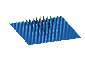
Figure 1. Case 1 plot of a Peregrine breather,  $|Q|$ from the NLS model (3.3),
  $M=0.01$ and
  $\varDelta =0$.

Figure 2. Case 1:  $M=0.01$,
  $\varDelta = 0$, (a) free surface plot from the modified Euler model, (b)
  $max(\eta )-min(\eta )$, (c) free surface plot from the NLS model, (d) free surface elevation at
  $t=9$ from both models.
The case of wind forcing with  $\varDelta =0.05$ is shown in figure 3. The free surface elevations in figures 3(a) and 3(c) from the modified Euler and FNLS models agree well in terms of group and phase velocities. Comparison of the free surface profiles at
  $t=9$ is shown in figure 3(d), the maximum amplitude grows as time increases. A plot of the maximum wave height defined by the difference between the maximum and minimum of the surface waves is shown in figure 3(b). The maximum wave height grows exponentially with approximately the growth rate
  $2\varDelta$, as predicted in Maleewong & Grimshaw (Reference Maleewong and Grimshaw2022). The main difference between the two models under wind forcing is that the fully nonlinear model predicts growing waves with wave breaking at a particular time, while the FNLS model predicts modulation of growing waves without wave breaking. It is possible that the FNLS model can predict the maximum wave height more than five times from the initial wave amplitude. But we cannot find a very-large-amplitude wave in the fully nonlinear model due to unstable and steep waves in the modified Euler code, that is, the program diverges. Here we use the term wave breaking to mean that in our simulations of the modified Euler system small-amplitude waves grow and become steep and then eventually become unstable, which we call wave breaking. We have not followed this beyond that point but this Euler code is capable of describing overturning waves, as in Cooker et al. (Reference Cooker, Peregrine, Vidal and Dold1990) and used by us in figure 11 of Grimshaw & Maleewong (Reference Grimshaw and Maleewong2013).

Figure 3. Case 1:  $M=0.01$,
  $\varDelta = 0.05$, (a) free surface plot from the modified Euler model, (b)
  $max(\eta )-min(\eta )$, (c) free surface plot from the FNLS model, (d) free surface elevation at
  $t=9$ from both models.
A case of higher wind forcing with  $\varDelta =0.1$ is shown in figure 4. Overall, the results are similar to the case of
  $\varDelta =0.05$, except very steep waves appear earlier. The fully nonlinear simulation breaks after
  $t>2$. Wind forcing in terms of the free surface gradient induces a large change at the crest of the free surface elevations. At that time, the FNLS model can still predict wave growth.

Figure 4. Case 1:  $M=0.01$,
  $\varDelta = 0.1$, (a) free surface plot from the modified Euler model, (b)
  $max(\eta )-min(\eta )$, (c) free surface plot from the FNLS model, (d) free surface elevation at
  $t=2$ from both models.
A case of higher amplitude of the envelope wave with  $M=0.02$ is shown in figure 5. Here we show only the case without wind forcing. The case with wind forcing is similar to the case of
  $M=0.01$. The evolution of the free surface obtained from the modified Euler and NLS models are shown in figures 5(a) and 5(c), respectively. The envelope waves travel with the predicted group velocity
  $c_g=0.5$. The profiles obtained from the two models are similar except that the maximum height in the fully nonlinear model grows at the early time step and then decreases in an oscillatory manner as time increases. In figure 5(d) the free surface profiles agree well in both phase and group velocities, the maximum wave height is of the same order as in the NLS model. The wave crest is higher while the wave trough is smaller and this may result in wave breaking later. We cannot simulate any fully nonlinear results for
  $M>0.03$ but we can simulate both the NLS and FNLS models for the cases of larger values of
  $M$. These weakly nonlinear models can predict large waves, but these are not physical as in the fully nonlinear simulation.

Figure 5. Case 1:  $M=0.02$,
  $\varDelta = 0$, (a) free surface plot from the modified Euler model, (b)
  $max(\eta )-min(\eta )$, (c) free surface plot from the NLS model, (d) free surface elevation at
  $t=49$ from both models.
Next we consider a case when  $\omega \neq 1$ and
  $k \neq 1$. We again consider the deep water limit when
  $F=1$ and
  $\sigma =1$. From the linear dispersion relation (2.11),
  $\omega ^2 = k$. We set
  $\omega =0.95$ and
  $k=0.9$. From (2.13), the pressure term in the dynamic boundary condition (2.9) of the modified Euler model can be written by (2.19). Thus, the growth rate
  $\varDelta$ is a connecting parameter between the modified Euler and FNLS models. We consider
  $\varDelta =0$ and
  $0.05$. The simulation starts at
  $t_0=-10$ and results are shown in figures 6 and 7. The initial amplitude
  $\eta (t_0)$ is small. The results from the two models are in good agreement for both
  $\varDelta =0$ and
  $\varDelta =0.05$. The results of the two models agree well when the value of
  $\omega$ is not far from
  $1$ and the initial wave amplitude is small. Note that the connecting parameter
  $\varDelta$ has the same value in both models. But if
  $\omega, k$ are smaller, then the magnitude of the pressure term in the modified Euler model grows due to the factor
  $1/\omega k$ in (2.19). With the same initial value for
  $\eta$, the modified Euler model will then predict larger growth rates than the FNLS model.

Figure 6. Case 1:  $M=0.01$,
  $\varDelta = 0$,
  $\omega =0.95$,
  $k=0.9$, (a) surface plot from the modified Euler model, (b)
  $max(\eta )-min(\eta )$, (c) surface plot from the NLS model, (d) free surface elevation at
  $t=40$ from both models.

Figure 7. Case 1:  $M=0.01$,
  $\varDelta = 0.05$,
  $\omega =0.95$,
  $k=0.9$, (a) surface plot from the modified Euler model, (b)
  $max(\eta )-min(\eta )$, (c) surface plot from the FNLS model, (d) free surface elevation at
  $t=8$ from both models.
4.2. Case 2
We will present just one representative case. We put  $M=0.02$ and
  $\hat {K}=0.05$, so that the soliton speed
  $V=0.1$ in the absence of wind forcing. Plots of the free surface profiles obtained from the modified Euler model and the NLS model are shown in figures 8(a) and 8(c), respectively. The maximum wave height is shown in figure 8(b) and both models show small oscillations, although the NLS model is nearly stationary. Comparison of the free surface profiles at
  $t=60$ is shown in figure 8(d) and are in good agreement. The NLS model has a slightly smaller wave amplitude than the modified Euler model. The magnitude of the crest and trough is nearly half of the maximum wave height, showing quite a linear wave.

Figure 8. Case 2:  $M=0.02$,
  $\varDelta = 0$, (a) surface plot from the modified Euler model, (b)
  $max(\eta )-min(\eta )$, (c) surface plot from the NLS model, (d) free surface elevation at
  $t=60$ from both models.
For the same value of  $M$, the simulations with wind forcing
  $\varDelta =0.05$ are shown in figure 9. The behaviour of the moving free surface elevation is similar to the case of
  $\varDelta =0$, except that the maximum wave height in figure 9(b) increases as time increases. Clearly the FNLS model predicts exponential growth which is the same result as discussed in Maleewong & Grimshaw (Reference Maleewong and Grimshaw2022). The modified Euler model shows increasing growth with oscillations as well but the maximum height is smaller, with developing asymmetry between crest and trough, more nonlinear behaviour than in the FNLS model. The modified Euler simulations can show some highly nonlinear effects in the form of a very steep wave with sharp gradients at the crests or troughs for other initial conditions; see figures 4, 7, 9(d) and figures 11, 13(d) below. These occur before the divergence of the fully nonlinear simulations (nearly breaking wave in our context). In contrast, the FNLSmodel can show some weakly nonlinear effects in terms of wave amplitude increase without the collapse of the free surface profile.

Figure 9. Case 2:  $M=0.02$,
  $\varDelta = 0.05$, (a) surface plot from the modified Euler model, (b)
  $max(\eta )-min(\eta )$, (c) surface plot from the FNLS model, (d) free surface elevation at
  $t=40$ from both models.
4.3. Case 3
This case has a more general initial condition than case 2 as the input wavenumber  $\gamma$ can be varied. If
  $\epsilon$ is small, more solitons will be generated, as presented in Maleewong & Grimshaw (Reference Maleewong and Grimshaw2022) and discussed above. When
  $\epsilon \ll 1$, there is a large disparity in time scales between the models which makes comparison of the numerical results difficult; the modified Euler model has then to run for a very long time, with the risk of wave breaking instability and a very high initial wave frequency, see the transform scales (2.21a–c). Hence, here we show only the case when
  $\epsilon =1$.
For the values of  $\gamma =0.2, M=0.02$ and in the case of
  $\varDelta =0$ a single soliton with constant amplitude emerges this is equivalent to an envelope wave in
  $\eta$ moving with a speed close to the group velocity
  $c_g$ in the modified Euler model. The evolution of
  $\eta$ from the two models over
  $0< t<100$ is shown in figures 10(a) and 10(c). They are in good agreement over the entire time simulation as seen from the comparison at
  $t=100$ in figure 10(d). The maximum wave heights from the two models are nearly equal and stationary over the whole time as expected.

Figure 10. Case 3:  $M=0.02$,
  $\varDelta = 0$, (a) surface plot from the modified Euler model, (b)
  $max(\eta )-min(\eta )$, (c) surface plot from the NLS model, (d) free surface elevation at
  $t=100$ from both models.
When there is wind forcing, the case of  $\varDelta =0.05$ is shown in figure 11. The simulation in the modified Euler model can be done only for
  $0< t<40$. As time increases, the wave amplitude increases. As shown in figure 11(d), the maximum wave height in the modified Euler model reaches about four times the height of the initial wave at
  $t=0$, resulting in very sharp and steep waves at
  $t=40$. After this time, the result from the Euler model diverges while those from the FNLS model remain convergent. The FNLS model predicts a growing wave amplitude. At
  $t = 40$, phase and group velocities from the two models are still in good agreement. The growth rates are shown in figure 11(b), clearly showing the expected exponential growth.

Figure 11. Case 3:  $M=0.02$,
  $\varDelta = 0.05$, (a) surface plot from the modified Euler model, (b)
  $max(\eta )-min(\eta )$, (c) surface plot from the FNLS model, (d) free surface elevation at
  $t=40$ from both models.
4.4. Case 4
The initial condition is a long-wave periodic perturbation with wavenumber  $\hat {K}$ and an amplitude
  $\alpha$. In the absence of wind forcing, this will lead to the modulation instability of a plane Stokes wave of amplitude
  $M$ and the formation of envelope solitons and breathers. We choose a large computational domain whose width is a multiple of
  $2{\rm \pi} /\hat {K}$ to maintain a periodic boundary condition without effects coming from the boundaries. Nevertheless, in the modified Euler model we insert a sponge layer for the initial value of
  $\eta$ to force its value to decay to zero at both ends. In the initial condition (3.6), we set
  $M=0.04$,
  $\hat {K}=0.04$ and
  $\alpha =0.5$. We are mainly concerned with the case of deep water and ensure that
  $\epsilon \hat {K} < \sqrt {2} |M|$ is satisfied so that the modulation instability will occur. The evolution of free surface profiles from the two models is shown in figure 12 when there is no wind forcing
  $\varDelta =0$. A train of envelope waves travels downstream (
 $x>0$) with a constant speed
  $c_g=0.5$, as shown in figures 12(a) and 12(c). Comparison of the free surface profiles at
  $t=100$ is shown in figure 12(d), while the NLS model shows only a small increasing change in the maximum wave height.

Figure 12. Case 4:  $M=0.04$,
  $\varDelta = 0$, (a) surface plot from the modified Euler model, (b)
  $max(\eta )-min(\eta )$, (c) surface plot from the NLS model, (d) free surface elevation at
  $t=100$ from both models.
The case of wind forcing with  $\varDelta =0.05$ is shown in figure 13. The train of envelope waves is directly perturbed by the wind forcing. As expected, the maximum wave height increases as time increases (figure 13b). We cannot obtain any fully nonlinear simulations when
  $t>12$, when the waves are very steep and sharp at the crests of the waves (figure 13d). The maximum wave height is greater than two times the initial wave height. After
  $t>12$, the FNLS model continues to predict a growing wave amplitude that is not too steep.

Figure 13. Case 4:  $M=0.04$,
  $\varDelta = 0.05$, (a) surface plot from the modified Euler model, (b)
  $max(\eta )-min(\eta )$, (c) surface plot from the FNLS model, (d) free surface elevation at
  $t=12$ from both models.
5. Summary and conclusions
In this paper our concern is with developing models for the analytical and numerical description of the evolution of water wave groups under the action of wind. Because of the numerical difficulties associated with the Kelvin–Helmholtz instability in an inviscid fully nonlinear two-fluid system such as air over water, we have presented instead a modified Euler model which is fully nonlinear for the water flow but in which the wind forcing from the air flow is severely approximated. Following the pioneering approach by Miles (Reference Miles1957), subsequently adopted by others such as the recent work by Kharif et al. (Reference Kharif, Kraenkel, Manna and Thomas2010), we prescribe a direct linear link (2.13) between the pressure at the air–water interface and the interface slope, thus avoiding the complications of a two-fluid simulation. In fact, of course, the sea state is far more complex than the configuration studied in our simulations; for instance, see the wind-generated sea states in the laboratory experiments of Toffoli et al. (Reference Toffoli, Proment, Salman, Monbaliu, Frascoli, Dafilis, Stramignoni, Forza, Manfrin and Onorato2017).
In the absence of wind forcing, the NLS equation is well established as a canonical model for weakly nonlinear wave groups. In the presence of wind forcing this is extended to a FNLS equation; see Leblanc (Reference Leblanc2007), Touboul et al. (Reference Touboul, Kharif, Pelinovsky and Giovanangeli2008), Kharif et al. (Reference Kharif, Kraenkel, Manna and Thomas2010), Montalvo et al. (Reference Montalvo, Kraenkel, Manna and Kharif2013), Onorato & Proment (Reference Onorato and Proment2012), Brunetti et al. (Reference Brunetti, Marchiando, Berti and Kasparian2014), Slunyaev et al. (Reference Slunyaev, Sergeeva and Pelinovsky2015), Grimshaw (Reference Grimshaw2018, Reference Grimshaw2019a,Reference Grimshawb), Maleewong & Grimshaw (Reference Maleewong and Grimshaw2022). Here, we impose a weakly nonlinear asymptotic expansion on the modified Euler system to derive the FNLS equation (2.15). The growth parameter  $\varDelta$ in the FNLS equation (2.15) is related to the pressure forcing term in the modified Euler system by the linear expression (2.19). With this connection, we simulate both models for the evolution of wave groups. In the relevant parameter regime, the outcomes agree very well. We note that the wind forcing term in the modified Euler system acts on the free surface slope, whereas in the FNLS equation it is expressed through the wave amplitude growth rate
  $\varDelta$. In the connecting formula (2.19) there is a factor
  $1/\omega k$ (in our dimensionless units). For the same free surface profile
  $\eta$ obtained from both models, there will be a large discrepancy in the forcing magnitude unless
  $1/\omega k \approx 1$. Hence, we have focused on cases close to the deep water limit when
  $\omega \approx 1, k \approx 1$ and so
  $F\approx 1$. In the full deep water limit,
  $\omega ^2=k, F=1$.
To examine the evolution of wave groups, we have considered four initial conditions, each of which in the absence of wind forcing would lead to contrasting representations of a wave group. In the terminology of the NLS equation these are (1) a Peregrine breather, (2) a soliton, (3) a slowly varying long-wave perturbation and (4) a long-wave periodic perturbation. In each case, envelope waves travel with a speed close to the linear group velocity  $c_g = 1/2$ (non-dimensional units) in the deep water limit. In the modified Euler simulations the initial condition for
  $\eta$ is given by (3.1) with the initial potential function approximated by linearised theory.
The initial free surface profile depends on  $\omega, k$ and
  $M$, all in non-dimensional units. The solutions are explored using two parameters,
  $M$ and
  $\varDelta$. Here
  $M$ is a non-dimensional measure of the initial carrier wave amplitude. In dimensional variables it is a measure of wave steepness. For a deep water
  $15$ s wave,
  $K = 0.019$ m
 $^{-1}$ and so a wave steepness
  $M = 0.02$ corresponds to a dimensional wave amplitude of about
  $M_d =1$ m, where
  $2M_d$ is the crest(trough) height above the undisturbed level. This initial amplitude could not be too large in the modified Euler simulations, as otherwise steep waves are generated with wave breaking.
The wind forcing is measured by  $(\varDelta )^{-1}$ which is a non-dimensional time for wave growth under wind action. In dimensional variables this is a time scale of
  $(\varDelta /\varOmega )^{-1}$ and is several carrier wave periods. For a
  $15$ s wave,
  $\varOmega = 0.42$ and so a typical
  $\varDelta = 0.05$ corresponds to about three wave periods. A more conventional measure of wind forcing is the wind speed at some height above the sea surface, in the Miles theory the critical level. This requires inter alia the determination of the parameter
  $\beta$ and the reference velocity
  $U_1$ in (2.18). This is beyond the scope of this paper as it requires specification of the wind profile in the air, but see Appendix A for a summary of how that might proceed. We note that Miles (Reference Miles1957) used a logarithmic wind shear profile and several turbulence parameters to estimate that
  $\beta \approx 10$. With this value and setting
  $KU_1/\varOmega =1$ for deep water waves with
  $k=1, \omega =1$, the expression (2.18) yields
  $\varDelta$ of order
  $0.01$. Miles (Reference Miles1957) used a smaller value of
  $KU_1/\varOmega$ in the range
  $0.25$–
 $0.5$ on the assumption that
  $U_1$ is near-surface wind velocity. We prefer our larger value for the evolution of a wave group under wind. Also, for a wave group, the requirement that the group velocity be real valued leads to enhanced growth rates; see Grimshaw (Reference Grimshaw2018). However, we note that in the expression (2.18)
  $\varDelta$ is quite sensitive to the values of
  $\beta$ and
  $U_1$. Hence, we have not followed this procedure and have avoided the selection of a wind shear profile.
In case (1) a Peregrine breather in the NLS model describes a free surface profile of a travelling envelope wave enclosing a carrier wave with amplitude  $M$. In the absence of wind forcing, both model simulations agree well. When wind forcing
  $\varDelta =0.05$ is applied, in both models the amplitude of the envelope wave grows. The maximum wave height defined by the difference between the maximum and minimum of the wave amplitude grows exponentially as time increases. The maximum wave height from the modified Euler model can grow to more than three times the initial state. Eventually, the crest wave in the modified Euler model becomes very steep and leads to wave breaking, while the wave amplitude in the FNLS model keeps growing with no wave breaking. We also simulated the case when the initial wave frequency
  $\omega = 0.95$, and both models provided similar results when
  $\varDelta =0$. When
  $\varDelta =0.05$, the modified Euler model predicted a higher maximum wave height than the FNLS model.
In case (2) a soliton represents a travelling envelope wave. In the absence of wind forcing, the modified Euler model showed travelling waves similar to the NLS model but with some small transients generated downstream. With wind forcing  $\varDelta = 0.05$ the results were similar but with the expected exponential growth in wave amplitude.
In case (3) for an initial condition of a slowly varying long-wave perturbation, both models agree well for  $\varDelta =0$ and
  $\varDelta =0.05$. The growth rate in terms of the maximum wave height is well matched. The modified Euler model eventually produces very steep waves, while the FNLS model continues to produce smoother wave crests. Since there is an envelope in the initial condition and we have applied wind forcing, we do not expect the theory for a plane periodic wave to apply quantitatively. The maximum amplitude in the modified Euler system can increase more than six times from the initial state. The wave amplitude in figure 11(d) does increase very rapidly over a short time after
  $t > 40$, but we stopped the simulation at
  $t = 40$ since the obtained results may not be realistic. To estimate this precisely, we need a very fine mesh and small time step to capture the near breaking wave, which is beyond the scope of this paper.
In case (4) the initial condition is a periodic long wave with modulation wavenumber  $\hat {K}$. In the absence of wind forcing a modulation instability occurs when
  $\epsilon \hat {K} < \sqrt {2} |M|$. Here we set
  $\epsilon =1$,
  $\hat {K}=0.04$ and
  $M=0.04$ and so we expected to see a modulation instability in this case. The modified Euler model clearly showed this in the maximum wave height while the NLS model showed a small modulation with increasing wave amplitude. During the modulation, the modified Euler model showed some asymmetry of wave group profiles. When wind forcing with
  $\varDelta =0.05$ is invoked, the expected exponential growth rate of the maximum wave height of both models agree. Here the simulation was stopped at
  $t=12$ when the maximum wave height for the modified Euler model was at most about two times the initial state, whereas in case 3 the simulation was run to
  $t= 40$.
Wave growth in our simulations comes from two mechanisms. One direct factor is our wind forcing term  $\varDelta$ which is a simplification of more complex mechanisms such as that due to Miles (Reference Miles1957). The predicted growth rate can be obtained from energy considerations, as in the FNLS model where it is expressed as
  $2\varDelta \epsilon ^{-1}$. The second mechanism to induce wave growth is a modulation instability as shown in case (4) in which the wave amplitude can grow in time even for the case without wind forcing
  $\varDelta =0$ when
  $\epsilon \hat {K} < \sqrt {2}|M|$.
There are two main issues outstanding in relating our results to observed ocean wind waves. The first is that we have taken absolutely minimal account of turbulence in the air flow. In the models we have presented, as in Miles (Reference Miles1957), air flow turbulence is expressed entirely through the parameter  $\beta$ in (2.13) and, as described in Appendix A, this is determined entirely by the choice of the wind shear profile. As in Miles (Reference Miles1957), a logarithmic profile is often chosen based on observations of air flow turbulence, but other representations are possible; see, for instance, Grimshaw (Reference Grimshaw2018). The remedy is either direct numerical simulation of an air–water system, well beyond our capability and intention, or more simply to invoke an eddy viscosity parametrisation, as used by Sajjadi, Hunt & Drullion (Reference Sajjadi, Hunt and Drullion2014), Sajjadi et al. (Reference Sajjadi, Drullion and Hunt2018) for instance. The parameter
  $\beta$ would then depend on the eddy viscosity parametrisation, but we will not explore this further here.
Second, the present study like many others has only one horizontal space dimension whereas observed wind-generated waves are two dimensional. Nevertheless, our present results are a guide to how wave groups initially form and, for long times, at best are limited to narrow wave tanks. The FNLS model can be readily extended to two dimensions, see, for instance, Toffoli et al. (Reference Toffoli, Gramstad, Trulsen, Monbalius, Bitner-Grerersen and Onorato2010) who compared experiments and numerical simulations of the water wave Euler equations with a modified extended NLS equation, and our recent study of a forced Benney–Roskes system, see Grimshaw (Reference Grimshaw2019b). This is the direction we intend to pursue. Extension of the modified Euler model to two horizontal space dimensions is also feasible in principle, but would need much more computational capacity than we have employed here.
Acknowledgements
We thank to the anonymous referees for useful suggestions.
Funding
R.G. was supported by the Leverhulme Trust through the award of a Leverhulme Emeritus Fellowship EM-2019-030.
Declaration of interests
The authors report no conflict of interest.
Author contributions
R.G. derived the theory and M.M. performed the simulations. All authors contributed equally to analysing data and reaching conclusions, and in writing the paper.
Appendix A. Linearised air flow equations
The linearised equations for the air flow are (see, for instance, Grimshaw Reference Grimshaw2018, Reference Grimshaw2019a)
 \begin{gather} \rho_a(D_U u+wU_{y})+p_x = 0 , \end{gather}
 \begin{gather}\rho_a D_U w + p_y+g\rho_a = 0 , \end{gather}
 \begin{gather}u_x+w_y = 0 , \end{gather}
 \begin{gather}\text{where } D_U = \frac{\partial }{\partial t} + U \frac{\partial }{\partial x } . \end{gather}
It is useful to introduce the vertical particle displacement  $\zeta$ defined in this linearised formulation by
 \begin{equation} D_U \zeta = w . \end{equation}
The substitution of  $w$ by
  $\zeta$ and eliminating
  $u, p$ yields a single equation for
  $\zeta$,
 \begin{equation} \{D_{U}^2 \zeta_y \}_y + \{D_{U}^2 \zeta \}_{xx} = 0 . \end{equation}
This equation is supplemented with the boundary conditions that as  $y \to \infty$,
  $\zeta \to 0$ and as
  $y \to 0$,
  $\zeta \to \eta$ and
  $p \to p_a$.
Equation (A6) can be solved with Fourier transforms in space and time yielding a means of expressing  $p_a$ in terms of
  $\eta$. Here we seek a simpler approach noting that our concern is with wave groups. Hence, we seek an asymptotic solution of (A6) in the form
 \begin{equation} \zeta = A(x,t)\phi(y)\exp{({\rm i}kx -{\rm i}kct)} + \hbox{c.c.} \end{equation}
Here  $A(x,t)$ is a slowly varying wave packet amplitude of a carrier wave with wavenumber
  $k$. Substitution of (A7) into (A6) yields at the leading order the modal equation
 \begin{equation} \{(c-U)^2 \phi_y \}_y - k^2 (c-U)^2 \phi = 0 . \end{equation}
The modal function  $\phi$ is normalised so that
  $\phi (y =0) = 1$ and then the required relation between
  $p_a$ and
  $\eta _x$ is given by
 \begin{gather} p_a = \rho_a c^2 A(x, t)\phi_{y}(0)\exp{({\rm i}kx -{\rm i}kct)} + \hbox{c.c.} , \end{gather}
 \begin{gather}\eta_x = {\rm i}kA(x,t) \exp{({\rm i}kx -{\rm i}kct)} + \hbox{c.c.} \end{gather}
Within this linear approximation elimination of  $A(x,t) \exp {(\textrm {i}kx -\textrm {i}kct)}$ yields the desired relation (2.13) in terms of
  $\phi _{y}(0)$. In particular, the parameter
  $\beta$ can now be obtained in terms of the available physical parameters; see Miles (Reference Miles1957) and many subsequent works.
Appendix B. Numerical method
Boundary integral methods are now commonly used to study two-dimensional unsteady free surface flows, especially the formation of steep waves. Here we use the numerical method presented by Grimshaw, Maleewong & Asavanant (Reference Grimshaw, Maleewong and Asavanant2009), based on that developed by Cooker et al. (Reference Cooker, Peregrine, Vidal and Dold1990), to solve numerically the system of nonlinear equations (2.6)–(2.9). Full details of the numerical method can be found in Grimshaw et al. (Reference Grimshaw, Maleewong and Asavanant2009), so here we summarise just the main steps.
Let  $\tilde {P}(s,t) = x(s, t) + i y(s , t)$ be the position of a point on the free surface, where
  $t$ is time and
  $s$ is a parameter indicating the location of a grid point. The complex velocity, defined by
  $w = \phi _x - i\phi _y$, is expressed in terms of the tangential (
 $s$) and normal (
 $n$) components to the free surface as
 \begin{equation} w = (\phi_s - i \phi_n) \frac{\tilde{P}^{*}_s}{|\tilde{P}_s|^2} , \end{equation}
where  $*$ represents the complex conjugate. Then, after using the Cauchy integral formula to express
  $w(z)$ in terms of points on the boundary, the continuity equation (2.6) and the bottom boundary condition (2.7) can be transformed into a matrix system at the discretization points as
 \begin{equation} {\rm \pi}\phi_{n}(s) ={-} \phi_{ss}(s) + \sum_{s^{'}=1}^{N} A(s,s^{'}) \phi_{s}(s^{'}) + \sum_{s^{'}=1}^{N} B(s,s^{'}) \phi_{n}(s^{'}) , \quad s = 1,2,\ldots, N, \end{equation}
where
 \begin{gather} A(s,s^{'}) = \hbox{Re} \left\{ \frac{-\tilde{P}_s} {\tilde{P}^{'}-\tilde{P}} + \frac{\tilde{P}_s}{\tilde{P}^{*'} - 2ih - \tilde{P}} \right\} \quad \text{if } s^{'} \neq s, \end{gather}
 \begin{gather}A(s,s^{'}) = \hbox{Re} \left\{ \frac{\tilde{P}_{ss}} {2\tilde{P}_{s}} + \frac{\tilde{P}_s}{\tilde{P}^{*'} - 2ih - \tilde{P}} \right\} \quad \text{if } s^{'} = s, \end{gather}
 \begin{gather}B(s,s^{'}) = \hbox{Im} \left\{ \frac{-\tilde{P}_s} {\tilde{P}^{'}- \tilde{P}} - \frac{\tilde{P}_s}{\tilde{P}^{*'} - 2ih - \tilde{P}} \right\} \quad \text{if } s^{'} \neq s, \end{gather}
 \begin{gather}B(s,s^{'}) = \hbox{Im} \left\{ \frac{\tilde{P}_{ss}} {2\tilde{P}_{s}} - \frac{\tilde{P}_s}{\tilde{P}^{*'} - 2ih - \tilde{P}} \right\} \quad \text{if } s^{'} = s . \end{gather}
 For an initial given shape of the free surface, we know  $\phi$,
  $\tilde {P}$ and
  $\tilde {P}^{*}$ at the points
  $s_i, i=1,\ldots,N$, while
  $\phi _s$ and
  $\phi _{ss}$ are approximated by the interpolation formula. Then the matrices
  $A(s,s^{'})$ and
  $B(s,s^{'})$ represent a known geometry of the problem. The linear system (B2) involves only the unknown
  $\phi _n$ at each point along the free surface and is solved iteratively. That is, we rewrite (B2) as
 \begin{gather} c = d + E c , \end{gather}
 \begin{gather}\text{where } c = \{ \phi_{n}(s^{'}) \} , \quad s^{'} = 1,2,\ldots,N , \end{gather}
 \begin{gather}d = \frac{1}{\rm \pi} \left\{ -\phi_{ss}(s) + \sum_{s^{'}=1}^{N} A(s,s^{'}) \phi_{n}(s^{'}) \right\} , \quad s = 1,2,\ldots,N , \end{gather}
 \begin{gather}E = \frac{1}{\rm \pi} \sum_{s^{'}=1}^{N} B(s,s^{'}) , \quad s = 1,2,\ldots,N . \end{gather}
Then we solve (B7) iteratively for the unknown vector  $c$,
$c$,
 \begin{equation} c_{m+1} = d + E c_{m} , \quad m = 1,2,\ldots , \end{equation}
where  $m$ denotes the
  $m$th iteration. For the first guess, we let
  $c_{1} = d$. The iterative process is terminated by measuring the error
  $|c_{m+1} - c_{m} | < Tol \approx 10^{-8}$. We have found
  $\phi _n$ at each mesh point along the free surface.
Next, we march the numerical solutions in time by solving (2.8) and (2.9). These equations are regarded as the first-order differential equations in  $t$ which can be solved numerically by a standard predictor–corrector method.


