


1 Introduction
Through its oscillatory motion across variable bottom topography, it is estimated that 1 TW of the barotropic tide is converted into internal gravity waves (Wunsch & Ferrari Reference Wunsch and Ferrari2004). Although in the near field the waves are manifest as vertically propagating beams, far from the generation site the internal tide is primarily composed of low modes. It is an open question how energy cascades from the large scales of the internal tides to small scales where mixing and dissipation can act. Some proposed mechanisms, as recently reviewed by MacKinnon et al. (Reference MacKinnon, Zhao, Whalen, Waterhouse, Trossman, Sun, St. Laurent, Simmons, Polzin and Pinkel2017), include interaction with topography and continental slopes, parametric subharmonic instability, interaction with mesoscale eddies, and nonlinear steepening of sufficiently large-amplitude internal tides.
Recent studies have demonstrated another mechanism for energy transfer to small scales whereby the self-interaction of internal waves in non-uniform stratification forces superharmonic disturbances. It will be shown in § 2.2 that this effect appears naturally from the equations of motion when the buoyancy frequency is non-uniform with depth. This mechanism was first recognised in the context of an internal wave beam interacting with the thermocline (Diamessis et al. Reference Diamessis, Wunsch, Delwiche and Richeter2014), and later through the self-interaction of the internal tide (Wunsch Reference Wunsch2015; Sutherland Reference Sutherland2016; Varma & Mathur Reference Varma and Mathur2017). The theoretical development of the latter studies assumed that the superharmonic response had twice the frequency of the internal tide (referred to hereafter as the ‘parent’ mode) with no temporal evolution of the superharmonic amplitude. However, simulations have shown that their time dependence need not be restricted to twice the frequency of the parent (Sutherland Reference Sutherland2016).

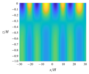
Figure 1. Snapshots from a fully nonlinear simulation showing (a) the full horizontal velocity field at times indicated and (b) the corresponding horizontal velocity field with the flow associated with the mode-1 parent mode removed. In this simulation, the background stratification is  $N^{2}(z)={N_{0}}^{2}\text{e}^{z/d}$ with
  $d=0.2H$ and Coriolis parameter
  $f=0.01N_{0}$. The simulation is initialised with a parent mode 1 with wavenumber
  $k=0.2/H$ and frequency
  $\unicode[STIX]{x1D714}=0.027N_{0}$. Note the growth of the superharmonic to a maximum amplitude at
  $N_{0}t\simeq 1000$, followed by decay to zero amplitude at
  $N_{0}t\simeq 2000$, corresponding to approximately 8.5 full periods of the parent mode. This process then repeats.
Wunsch (Reference Wunsch2017) explored this theoretically for a piecewise-constant stratification profile, and found a near-resonant initial growth of the superharmonic response, comparing the interaction between the internal tide and superharmonics to that of a forced harmonic oscillator whereby the nonlinear self-interaction of the parent excites a superharmonic with frequency close to its natural unforced frequency. However, this study assumed that, after a period of initial growth, the oscillating transients would be damped by viscosity and the system would reach steady state.
Motivating the present work is the result of long-time numerical simulations similar to those of Sutherland (Reference Sutherland2016) of horizontally periodic mode-1 internal tides in non-uniform stratification typical of the ocean, which show that superharmonics do not grow to steady state but instead periodically grow and decay, as shown in figure 1. Here we develop a weakly nonlinear (WNL) theory to explain this phenomenon. In § 2.1 we introduce a theoretical framework for the parent internal tide in arbitrary stratification,  $N^{2}(z)$. In § 2.2 we develop a time-dependent theory for the generation of superharmonics, using a slow-/fast-time-scale separation to extend the evolution beyond the initial growth phase considered by Wunsch (Reference Wunsch2017). In § 2.3 this is extended to a WNL theory incorporating energy transfer between the parent and superharmonic. Numerical simulations employing realistic exponential oceanic stratification are introduced in § 3 and compared to the theoretical results. A summary of results is given in § 4, wherein the theory is applied to the examination of internal tides emanating from the Hawaiian islands.
2 Theory
The fully nonlinear equation for an inviscid, incompressible Boussinesq fluid on the  $f$-plane with spanwise-invariant flow is written as a linear operator acting on the streamfunction,
  $\unicode[STIX]{x1D713}$, being forced by nonlinear terms as follows (Wunsch Reference Wunsch2017):
 $$\begin{eqnarray}\unicode[STIX]{x1D6FB}^{2}\unicode[STIX]{x1D713}_{tt}+f^{2}\unicode[STIX]{x1D713}_{zz}+N^{2}\unicode[STIX]{x1D713}_{xx}={\mathcal{N}}(\unicode[STIX]{x1D713},v,b),\end{eqnarray}$$
 in which subscripts denote partial derivatives,  $N^{2}(z)$ is the background stratification,
  $f$ is the (constant) Coriolis parameter,
  $b$ is the buoyancy,
  $v$ is the spanwise velocity, and the along-stream and vertical velocities are given in terms of the streamfunction, respectively, by
  $u=-\unicode[STIX]{x1D713}_{z}$ and
  $w=\unicode[STIX]{x1D713}_{x}$. The nonlinear forcing is given explicitly by
 $$\begin{eqnarray}{\mathcal{N}}=\unicode[STIX]{x1D735}\boldsymbol{\cdot }[\unicode[STIX]{x2202}_{t}(\boldsymbol{u}\unicode[STIX]{x1D701})-\unicode[STIX]{x2202}_{x}(\boldsymbol{u}b)+f\unicode[STIX]{x2202}_{z}(\boldsymbol{u}v)],\end{eqnarray}$$
 in which  $\boldsymbol{u}=(u,w)$ and
  $\unicode[STIX]{x1D701}=-\unicode[STIX]{x1D6FB}^{2}\unicode[STIX]{x1D713}$.
2.1 Parent mode
We seek horizontally periodic solutions of a single mode vertically bounded by  $-H\leqslant z\leqslant 0$. In terms of the streamfunction,
 $$\begin{eqnarray}\unicode[STIX]{x1D713}^{(1)}(x,z,t)=\frac{1}{2}\unicode[STIX]{x1D6FC}\frac{\unicode[STIX]{x1D714}d}{k}\hat{\unicode[STIX]{x1D713}}_{1}(z)\text{e}^{\text{i}\unicode[STIX]{x1D719}}+\text{c.c.},\end{eqnarray}$$
 in which  $\unicode[STIX]{x1D719}\equiv kx-\unicode[STIX]{x1D714}t$,
  $k$ is the prescribed horizontal wavenumber of the parent mode,
  $\unicode[STIX]{x1D714}$ is its frequency,
  $d$ is a characteristic length scale of the stratification profile
  $N^{2}(z)$,
  $\text{c.c.}$ is the complex conjugate, and the vertical structure function
  $\hat{\unicode[STIX]{x1D713}}(z)$ is normalised so that
  $\max |\hat{\unicode[STIX]{x1D713}}(z)|=1$. The non-dimensional amplitude
  $\unicode[STIX]{x1D6FC}$ is a measure of the maximum horizontal flow associated with the waves compared with their phase speed. The superscript on
  $\unicode[STIX]{x1D713}$ and subscript on
  $\hat{\unicode[STIX]{x1D713}}$ correspond to a horizontal wavenumber
  $1k$. Substituting (2.3) into (2.1) and neglecting the nonlinear terms gives the eigenvalue problem for
  $\hat{\unicode[STIX]{x1D713}}_{1}$:
 $$\begin{eqnarray}{\hat{\unicode[STIX]{x1D713}}_{1}}^{\prime \prime }+k^{2}\frac{N^{2}(z)-\unicode[STIX]{x1D714}^{2}}{\unicode[STIX]{x1D714}^{2}-f^{2}}\hat{\unicode[STIX]{x1D713}}_{1}=0,\end{eqnarray}$$
 with  $\hat{\unicode[STIX]{x1D713}}(0)=\hat{\unicode[STIX]{x1D713}}(-H)=0$. For prescribed
  $k$, the solution gives a set of eigenfunctions
  $\hat{\unicode[STIX]{x1D713}}_{1}$ with corresponding frequencies
  $\unicode[STIX]{x1D714}$. Generally, equation (2.4) is solved numerically using a Galerkin method. In what follows, we only consider a vertical mode-1 parent wave for which
  $\hat{\unicode[STIX]{x1D713}}_{1}$ is non-negative for all
  $z$.
$z$.
Given the streamfunction of the parent mode, the polarisation relations give  $u^{(1)}=-\unicode[STIX]{x2202}_{z}\unicode[STIX]{x1D713}^{(1)}$,
  $w^{(1)}=\unicode[STIX]{x2202}_{x}\unicode[STIX]{x1D713}^{(1)}$, the spanwise velocity
  $v^{(1)}=\frac{1}{2}\unicode[STIX]{x1D6FC}\hat{v}_{1}\text{e}^{\text{i}\unicode[STIX]{x1D719}}+\text{c.c.}$ and buoyancy
  $b^{(1)}=\frac{1}{2}\unicode[STIX]{x1D6FC}\hat{b}_{1}\text{e}^{\text{i}\unicode[STIX]{x1D719}}+\text{c.c.}$, in which
 $$\begin{eqnarray}\hat{v}_{1}=\text{i}\,\frac{fd}{k}\hat{\unicode[STIX]{x1D713}}_{1}^{\prime },\quad \hat{b}_{1}=dN^{2}\hat{\unicode[STIX]{x1D713}}_{1}.\end{eqnarray}$$
2.2 Superharmonic response
Consider now the nonlinear terms in (2.1). The  $O(\unicode[STIX]{x1D6FC})$ parent mode self-interacts in these terms to create an
  $O(\unicode[STIX]{x1D6FC}^{2})$ forcing upon the linear operator acting on the
  $O(\unicode[STIX]{x1D6FC}^{2})$ correction to the streamfunction. This forcing has a term that is proportional to
  $\text{e}^{0\text{i}\unicode[STIX]{x1D719}}$ that forces a mean flow, and a term that is proportional to
  $\text{e}^{2\text{i}\unicode[STIX]{x1D719}}$ that forces a superharmonic with twice the horizontal wavenumber of the parent. Although the forcing is also at twice the frequency of the parent, we will show that the superharmonic response has a temporal evolution that is not necessarily at frequency
  $2\unicode[STIX]{x1D714}$.
Using the polarisation relations, the nonlinear forcing terms are calculated using (2.4) to replace second derivatives of  $\hat{\unicode[STIX]{x1D713}}_{1}$. Substituting these into (2.1) gives
 $$\begin{eqnarray}\unicode[STIX]{x1D6FB}^{2}\unicode[STIX]{x1D713}_{tt}+f^{2}\unicode[STIX]{x1D713}_{zz}+N^{2}\unicode[STIX]{x1D713}_{xx}={\mathcal{G}}_{0}(z)+{\mathcal{G}}_{2}(z)\text{e}^{2\text{i}\unicode[STIX]{x1D719}}+\text{c.c.},\end{eqnarray}$$
where
 $$\begin{eqnarray}\displaystyle & \displaystyle {\mathcal{G}}_{0}=-\frac{\unicode[STIX]{x1D6FC}^{2}k\unicode[STIX]{x1D714}d^{2}f^{2}}{4(\unicode[STIX]{x1D714}^{2}-f^{2})}\left(2(N^{2}-\unicode[STIX]{x1D714}^{2})\frac{\unicode[STIX]{x2202}}{\unicode[STIX]{x2202}z}|\hat{\unicode[STIX]{x1D713}}_{1}|^{2}+(N^{2})^{\prime }|\hat{\unicode[STIX]{x1D713}}_{1}|^{2}\right), & \displaystyle\end{eqnarray}$$
 $$\begin{eqnarray}\displaystyle & \displaystyle {\mathcal{G}}_{2}=\frac{\unicode[STIX]{x1D6FC}^{2}k\unicode[STIX]{x1D714}d^{2}(4\unicode[STIX]{x1D714}^{2}-f^{2})(N^{2})^{\prime }}{4(\unicode[STIX]{x1D714}^{2}-f^{2})}\hat{\unicode[STIX]{x1D713}}_{1}^{2}. & \displaystyle\end{eqnarray}$$
This equation is equivalent to the result of Wunsch (Reference Wunsch2017) when viscosity is neglected in equation (2.9) therein. We make this assumption throughout, justified by the large length scales and slow time scales of the parent and superharmonic internal modes. Viscous dissipation will also act to a similar extent on the parent and superharmonic, so we expect that it will not fundamentally modify their interactions.
In the case of uniform stratification and no background rotation, there is no forcing through self-interaction, which is a consequence of monochromatic internal waves being an exact solution of the fully nonlinear equations of motion.
To be justified later, we neglect the forcing of the mean flow (through  ${\mathcal{G}}_{0}$), focusing upon the forcing of superharmonics by a parent mode in non-uniform stratification through
 $$\begin{eqnarray}\unicode[STIX]{x1D6FB}^{2}\unicode[STIX]{x1D713}_{tt}^{(2)}+f^{2}\unicode[STIX]{x1D713}_{zz}^{(2)}+N^{2}\unicode[STIX]{x1D713}_{xx}^{(2)}={\mathcal{G}}_{2}(z)\text{e}^{2\text{i}\unicode[STIX]{x1D719}}+\text{c.c.}\end{eqnarray}$$
The streamfunction of the superharmonic is assumed to evolve in time and space according to
 $$\begin{eqnarray}\unicode[STIX]{x1D713}^{(2)}=\frac{1}{2}\unicode[STIX]{x1D6FC}^{2}\frac{\unicode[STIX]{x1D714}d}{k}\tilde{\unicode[STIX]{x1D713}}_{2}(z,T)\text{e}^{2\text{i}\unicode[STIX]{x1D719}}+\text{c.c.}\end{eqnarray}$$
 Crucially, its time dependence is allowed to vary not only with frequency  $2\unicode[STIX]{x1D714}$ (in the
  $\text{e}^{2\text{i}\unicode[STIX]{x1D719}}$ term), but also on a slow time scale
  $T=\unicode[STIX]{x1D716}t$, with
  $\unicode[STIX]{x1D716}\ll 1$ to be defined explicitly below. This is intended to capture the growth and decay of superharmonics, which was observed in simulations to occur on time scales much longer than
  $\unicode[STIX]{x1D714}^{-1}$. Note that this slow-time-scale assumption need not be made a priori, but is made here for convenience and justified later. We construct the following expansion in terms of vertical structure functions
  $\hat{\unicode[STIX]{x1D713}}_{2,j}$:
 $$\begin{eqnarray}\tilde{\unicode[STIX]{x1D713}}_{2}(z,T)=\mathop{\sum }_{j=1}^{\infty }a_{j}(T)\hat{\unicode[STIX]{x1D713}}_{2,j}(z).\end{eqnarray}$$
 For each  $j$,
$j$,  $\hat{\unicode[STIX]{x1D713}}_{2,j}(z)$ is the vertical structure of the
  $j$th mode of the unforced superharmonic, which has corresponding frequency
  $\unicode[STIX]{x1D714}_{2,j}$. Explicitly,
  $\hat{\unicode[STIX]{x1D713}}_{2,j}$ satisfies (cf. (2.4))
 $$\begin{eqnarray}\hat{\unicode[STIX]{x1D713}}_{2,j}^{\prime \prime }+4k^{2}\frac{N^{2}-\unicode[STIX]{x1D714}_{2,j}^{2}}{\unicode[STIX]{x1D714}_{2,j}^{2}-f^{2}}\hat{\unicode[STIX]{x1D713}}_{2,j}=0.\end{eqnarray}$$
 The expansion (2.11) is similar to the eigenvalue expansion (2.10) of Wunsch (Reference Wunsch2017), although here we have made the slow-time-scale assumption and continue with arbitrary background stratification. Applying Sturm–Liouville theory to (2.12), the set of eigenfunctions  $\hat{\unicode[STIX]{x1D713}}_{2,j}$ can be shown to be orthogonal with respect to the weight function
  $W(z)\equiv N^{2}-f^{2}$ so that
 $$\begin{eqnarray}\int _{-H}^{0}\hat{\unicode[STIX]{x1D713}}_{2,j}(z)\hat{\unicode[STIX]{x1D713}}_{2,l}(z)W(z)\,\text{d}z=\unicode[STIX]{x1D6FF}_{j,l}\int _{-H}^{0}(\hat{\unicode[STIX]{x1D713}}_{2,j}(z))^{2}W(z)\,\text{d}z.\end{eqnarray}$$
 Thus, substituting (2.10) and (2.11) into (2.9), multiplying through by another basis function, integrating over  $z\in [-H,0]$ and using (2.13) gives
 $$\begin{eqnarray}\unicode[STIX]{x1D716}^{2}\ddot{a}_{j}-4\text{i}\unicode[STIX]{x1D714}\unicode[STIX]{x1D716}{\dot{a}}_{j}-4\unicode[STIX]{x1D714}^{2}\unicode[STIX]{x1D6E5}_{j}a_{j}=-2\unicode[STIX]{x1D714}^{2}M_{j},\end{eqnarray}$$
 where  ${\dot{a}}$ denotes
  $\unicode[STIX]{x2202}a/\unicode[STIX]{x2202}T$ and
  $M_{j}$ and
  $\unicode[STIX]{x1D6E5}_{j}$ are constants defined by
 $$\begin{eqnarray}M_{j}=d\frac{4\unicode[STIX]{x1D714}^{2}-f^{2}}{4(\unicode[STIX]{x1D714}^{2}-f^{2})}\frac{\unicode[STIX]{x1D714}_{2,j}^{2}-f^{2}}{4\unicode[STIX]{x1D714}^{2}}\frac{\displaystyle \int _{-H}^{0}(N^{2})^{\prime }\hat{\unicode[STIX]{x1D713}}_{1}^{2}\hat{\unicode[STIX]{x1D713}}_{2,j}\,\text{d}z}{\displaystyle \int _{-H}^{0}(N^{2}-f^{2})\hat{\unicode[STIX]{x1D713}}_{2,j}^{2}\,\text{d}z},\quad \unicode[STIX]{x1D6E5}_{j}=\frac{4\unicode[STIX]{x1D714}^{2}-\unicode[STIX]{x1D714}_{2,j}^{2}}{4\unicode[STIX]{x1D714}^{2}}.\end{eqnarray}$$
 Notice that  $\unicode[STIX]{x1D6E5}_{j}$ is effectively the normalised difference between the superharmonic forcing frequency
  $2\unicode[STIX]{x1D714}$ and natural frequency
  $\unicode[STIX]{x1D714}_{2,j}$ of the unforced superharmonic vertical mode
  $j$.
$j$.
The first term of (2.14) is  $O(\unicode[STIX]{x1D716})$ smaller than the second term, and is neglected to leading order in
  $\unicode[STIX]{x1D716}$. The evolution of
  $a_{j}$ at leading order in
  $\unicode[STIX]{x1D716}$ is given by
 $$\begin{eqnarray}{\dot{a}}_{j}-\frac{\text{i}\unicode[STIX]{x1D714}\unicode[STIX]{x1D6E5}_{j}}{\unicode[STIX]{x1D716}}a_{j}=-\frac{\text{i}\unicode[STIX]{x1D714}M_{j}}{2\unicode[STIX]{x1D716}}.\end{eqnarray}$$
 The steady solution (e.g. that considered by Wunsch (Reference Wunsch2015) and Varma & Mathur (Reference Varma and Mathur2017)) can be found as a special case of (2.16) using the initial condition  $a_{j}(0)=M_{j}/2\unicode[STIX]{x1D6E5}_{j}$. Here we impose the initial condition
  $a_{j}(0)=0$ so that there is a pure parent mode at
  $t=0$. The solution to (2.16) is then
 $$\begin{eqnarray}a_{j}=\frac{M_{j}}{2\unicode[STIX]{x1D6E5}_{j}}(1-\text{e}^{(\text{i}\unicode[STIX]{x1D714}\unicode[STIX]{x1D6E5}_{j}/\unicode[STIX]{x1D716})T}).\end{eqnarray}$$
 For internal tides in realistic oceanic stratification for which  $N^{2}$ is monotonically increasing with height over most of the ocean depth, two effects conspire to ensure that most of the forcing results in excitation of a mode-1 superharmonic by a mode-1 parent (i.e.
  $a_{j}\ll a_{1}$ for
  $j>1$).
Firstly, the integrand in the numerator of (2.15) is single-signed only in the case with  $j=1$, suggesting
  $M_{j}$ is largest for
  $j=1$. For example, when
  $j=2$, the integrand
  $(N^{2})^{\prime }\hat{\unicode[STIX]{x1D713}}_{1}^{2}\hat{\unicode[STIX]{x1D713}}_{2,j}$ is not single-signed and much of the integral will cancel so that
  $M_{2}\ll M_{1}$. A realistic oceanic stratification will include a surface mixed layer in which
  $(N^{2})^{\prime }$ changes sign. But, since
  $\hat{\unicode[STIX]{x1D713}}_{1}=0$ at the surface, this effect is minimal when
  $(N^{2})^{\prime }$ is multiplied by
  $\hat{\unicode[STIX]{x1D713}}_{1}$ in the integrand because the vertical structure function goes to zero near the surface.

Figure 2. Twice the parent dispersion relation  $2\unicode[STIX]{x1D714}(k)/N_{0}$ and the dispersion relation of the unforced superharmonic
  $\unicode[STIX]{x1D714}(2k)/N_{0}$ for the cases (a)
  $f=0$ and (b)
  $f=0.01N_{0}$.
Secondly,  $\unicode[STIX]{x1D6E5}_{1}$ is small for realistic oceanic parameters because
  $2\unicode[STIX]{x1D714}(k)\simeq \unicode[STIX]{x1D714}(2k)$. This is illustrated in figure 2 (similar to figure 2 of Wunsch (Reference Wunsch2017)) where the superharmonic dispersion relation
  $\unicode[STIX]{x1D714}(2k)$ and twice the parent dispersion relation
  $2\unicode[STIX]{x1D714}(k)$ are plotted for the cases
  $f=0$ and
  $f=0.01N_{0}$. In each case, the (normalised) vertical separation between the two curves for each
  $k$ scales with
  $\unicode[STIX]{x1D6E5}_{1}$. For values of
  $k$ representative of low-mode internal tides,
  $\unicode[STIX]{x1D714}(k)$ is near-linear and
  $\unicode[STIX]{x1D6E5}_{1}$ is small. Since
  $\unicode[STIX]{x1D714}(0)=f$, in the case
  $f=0$ the dispersion relation intersects the origin and
  $\unicode[STIX]{x1D714}(2k)$ is even closer to
  $2\unicode[STIX]{x1D714}(k)$. Hence, from (2.15),
 $$\begin{eqnarray}0\lesssim \unicode[STIX]{x1D6E5}_{1}\ll \unicode[STIX]{x1D6E5}_{j},\quad j>1.\end{eqnarray}$$
 The dominance of superharmonics being excited with near-pure mode-1 structure is a robust result for realistic values of the relative Coriolis parameter, parent mode horizontal wavenumber and for various representative profiles of the ocean stratification. This is illustrated in table 1, which gives percentage values of  $\max |a_{2}|/\!\max |a_{1}|=(M_{1}/\unicode[STIX]{x1D6E5}_{1})/(M_{2}/\unicode[STIX]{x1D6E5}_{2})$, being the relative amplitude of the mode-2 to the mode-1 component of the superharmonic in the expansion (2.11), as computed for three different background stratification profiles typically used to model the ocean. The choice of stratification profile does not modify the result; for various realistic values of
  $f$ and
  $k$, the mode-2 component is less than 5 % of the mode-1 component. For
  $f=0$ (at the equator) the dominance of the mode-1 component is more pronounced, with the mode-2 component being less than 0.5 % that of mode 1.
Table 1. Maximum amplitude of the mode-2 component of the superharmonic as a percentage of the mode-1 component. Profile 1:  $N^{2}=N_{0}^{2}\text{e}^{z/d}$. Profile 2: As in profile 1, with a mixed layer of depth
  $z_{mix}$ given by
  $N^{2}(z)=\frac{1}{2}N_{0}^{2}\text{e}^{z/d}[1-\tanh ((z+z_{mix})/\unicode[STIX]{x1D70E})]$ with
  $\unicode[STIX]{x1D70E}=0.001H$ and
  $d=0.2H$. Profile 3:
  $N^{2}=N_{0}^{2}d^{2}/(d-z)^{2}$.

It is possible to create a non-realistic stratification in which the mode-1 dominance of the superharmonic breaks down. For example, the symmetric top-hat stratification used by Sutherland (Reference Sutherland2016) has  $M_{1}=0$, since in (2.15),
  $(N^{2})^{\prime }$ is odd and
  $\hat{\unicode[STIX]{x1D713}}_{1}$ even about the midpoint in depth. In this case, the superharmonics generated have a higher vertical wavenumber (Sutherland Reference Sutherland2016).
The dominance of  $a_{1}$ is now used to simplify the expression for the superharmonic at leading order. The slow-time parameter is defined such that
 $$\begin{eqnarray}\unicode[STIX]{x1D716}\equiv \unicode[STIX]{x1D6E5}_{1}=\frac{4\unicode[STIX]{x1D714}(k)^{2}-\unicode[STIX]{x1D714}(2k)^{2}}{4\unicode[STIX]{x1D714}(k)^{2}}.\end{eqnarray}$$
 Writing  $a\equiv a_{1}$,
  $\hat{\unicode[STIX]{x1D713}}_{2}\equiv \hat{\unicode[STIX]{x1D713}}_{2,1}$,
  $\hat{\unicode[STIX]{x1D713}}_{1}\equiv \hat{\unicode[STIX]{x1D713}}_{1,1}$,
  $\unicode[STIX]{x1D714}_{2,1}\equiv \unicode[STIX]{x1D714}_{2}$,
  $M\equiv M_{1}$ and
  $\unicode[STIX]{x1D6E5}\equiv \unicode[STIX]{x1D6E5}_{1}$, the structure and evolution of the dominantly excited superharmonic is given by
 $$\begin{eqnarray}\unicode[STIX]{x1D713}^{(2)}=\frac{1}{2}\unicode[STIX]{x1D6FC}^{2}\frac{\unicode[STIX]{x1D714}d}{k}a(T)\hat{\unicode[STIX]{x1D713}}_{2}\text{e}^{2\text{i}\unicode[STIX]{x1D719}}+\text{c.c.},\quad a(T)=\frac{M}{2\unicode[STIX]{x1D716}}(1-\text{e}^{\text{i}\unicode[STIX]{x1D714}T}),\quad T=\unicode[STIX]{x1D716}t.\end{eqnarray}$$
 The superharmonic therefore evolves periodically on two time scales, one oscillating at the fast forcing frequency  $2\unicode[STIX]{x1D714}$ and the other describing the slow growth and decay at a ‘beat’ frequency
  $\unicode[STIX]{x1D716}\unicode[STIX]{x1D714}$.
This evolution is an extension of the ‘near-resonance’ described in Wunsch (Reference Wunsch2017). As  $\unicode[STIX]{x1D716}\rightarrow 0$, the forcing frequency approaches the natural frequency of the mode-1 superharmonic, and the system is near resonance. The maximum amplitude of the superharmonic becomes larger with a longer period as
  $\unicode[STIX]{x1D716}\rightarrow 0$, until in the limit
  $\unicode[STIX]{x1D716}=0$ the growth is linear and true resonance occurs. Therefore
  $\unicode[STIX]{x1D716}$ is a measure of how far the system is from triadic resonance, as reviewed by Staquet & Sommeria (Reference Staquet and Sommeria2002).
The values of  $\unicode[STIX]{x1D716}$,
  $M$ and other quantities for various realistic parameter regimes in an exponential stratification are shown in table 2. In particular, note that
  $\unicode[STIX]{x1D716}$ decreases as
  $f$ decreases whilst
  $M$ stays relatively constant, implying that the maximum superharmonic amplitude is greater at low latitudes – a conclusion also reached by Wunsch (Reference Wunsch2017) for a piecewise-constant stratification profile.
Table 2. Values of the frequency  $\unicode[STIX]{x1D714}/N_{0}$,
  $\unicode[STIX]{x1D716}$ (as defined by (2.19)),
  $D$ (as defined by (2.24)–(2.25)),
  $M$ (as defined by (2.15)) and
  $D/M$ for given Coriolis parameter
  $f/N_{0}$, parent wavenumber
  $kH$ and stratification length scale
  $d/H$, where the stratification is given by
  $N^{2}=N_{0}^{2}\text{e}^{z/d}$.

Repeating the above analysis for the mean flow would recover an  $O(\unicode[STIX]{x1D6FC}^{2})$ solution. By comparison with (2.20), it can be seen that the mean flow is
  $O(\unicode[STIX]{x1D716})$ smaller than the superharmonic because it does not exhibit the same near-resonant behaviour. It is thus neglected at leading order in
  $\unicode[STIX]{x1D716}$ (though see van den Bremer, Yassin & Sutherland (Reference van den Bremer, Yassin and Sutherland2019)).
2.3 Weakly nonlinear theory
The expression (2.20) predicts that the ratio of the maximum superharmonic amplitude to the parent amplitude is given by  $\unicode[STIX]{x1D6FC}/\unicode[STIX]{x1D716}$. This theory assumes that the parent maintains its initial energy, never losing energy to the superharmonic. It is therefore valid only in the limit
  $\unicode[STIX]{x1D6FC}/\unicode[STIX]{x1D716}\ll 1$; that is, in the case that the superharmonic does not grow large enough to extract significant energy from the parent. However, for superharmonics that grow to finite amplitude, the modification of the parent due to the growth of the superharmonic must be taken into account.
We construct a coupled system comprising the parent and superharmonic only, with total streamfunction given by
 $$\begin{eqnarray}\unicode[STIX]{x1D713}=\frac{1}{2}\frac{\unicode[STIX]{x1D714}d}{k}(\unicode[STIX]{x1D6FC}p(T)\hat{\unicode[STIX]{x1D713}}_{1}\text{e}^{\text{i}\unicode[STIX]{x1D719}}+\unicode[STIX]{x1D6FC}^{2}a(T)\hat{\unicode[STIX]{x1D713}}_{2}\text{e}^{2\text{i}\unicode[STIX]{x1D719}})+\text{c.c.},\end{eqnarray}$$
 where  $p(T)$ is the (complex-valued) parent amplitude (previously taken to be 1) and
  $a(T)$ is again the superharmonic amplitude, not necessarily as defined in (2.20). We immediately consider only the mode-1 components of the parent and superharmonic, due to the strong amplification of the mode 1 as described in § 2.2.
We begin by modifying the original equation (2.16) for the superharmonic forced by parent self-interaction to include the effect of the changing parent amplitude. Under the assumption that  $\unicode[STIX]{x1D716}{\dot{p}}\ll \unicode[STIX]{x1D714}p$ and noticing that the polarisation relations (2.5) remain valid for the now-varying parent at leading order in
  $\unicode[STIX]{x1D716}$, equation (2.16) for
  $j=1$ becomes simply
 $$\begin{eqnarray}{\dot{a}}-\text{i}\unicode[STIX]{x1D714}a=-\text{i}\unicode[STIX]{x1D714}\frac{M}{2\unicode[STIX]{x1D716}}p^{2}.\end{eqnarray}$$
 The equation for the forcing of the parent due to the interaction of the parent and superharmonic can now be derived. Using the same methodology as in the consideration above of the parent self-interaction gives, at leading order in  $\unicode[STIX]{x1D716}$,
 $$\begin{eqnarray}{\dot{p}}=-\text{i}\unicode[STIX]{x1D714}\unicode[STIX]{x1D6FC}^{2}\frac{D}{2\unicode[STIX]{x1D716}}ap^{\ast },\end{eqnarray}$$
 where  $p^{\ast }$ is the complex conjugate of
  $p$, and
  $D$ is a constant given by
 $$\begin{eqnarray}D=\frac{\displaystyle (\unicode[STIX]{x1D714}^{2}-f^{2})\int _{-H}^{0}{\mathcal{D}}(z)\hat{\unicode[STIX]{x1D713}}_{1}\,\text{d}z}{\displaystyle \unicode[STIX]{x1D714}^{2}\int _{-H}^{0}(N^{2}-f^{2})\hat{\unicode[STIX]{x1D713}}_{1}^{2}\,\text{d}z},\end{eqnarray}$$
with
 $$\begin{eqnarray}\displaystyle {\mathcal{D}}(z) & = & \displaystyle \frac{d}{2}\left[\hat{\unicode[STIX]{x1D713}}_{1}\hat{\unicode[STIX]{x1D713}}_{2}(N^{2})^{\prime }\left(3-\frac{4\unicode[STIX]{x1D714}^{2}+2f^{2}}{\unicode[STIX]{x1D714}_{2}^{2}-f^{2}}\right)-2f^{2}\hat{\unicode[STIX]{x1D713}}_{1}\hat{\unicode[STIX]{x1D713}}_{2}^{\prime }\frac{N^{2}-\unicode[STIX]{x1D714}^{2}}{\unicode[STIX]{x1D714}^{2}-f^{2}}\right.\nonumber\\ \displaystyle & & \displaystyle -\,8f^{2}\hat{\unicode[STIX]{x1D713}}_{1}^{\prime }\hat{\unicode[STIX]{x1D713}}_{2}\frac{N^{2}-\unicode[STIX]{x1D714}_{2}^{2}}{\unicode[STIX]{x1D714}_{2}^{2}-f^{2}}-2f^{2}(\hat{\unicode[STIX]{x1D713}}_{1}^{\prime }\hat{\unicode[STIX]{x1D713}}_{2}+\hat{\unicode[STIX]{x1D713}}_{1}\hat{\unicode[STIX]{x1D713}}_{2}^{\prime })\left(\frac{N^{2}-\unicode[STIX]{x1D714}^{2}}{\unicode[STIX]{x1D714}^{2}-f^{2}}+\frac{N^{2}-\unicode[STIX]{x1D714}_{2}^{2}}{\unicode[STIX]{x1D714}_{2}^{2}-f^{2}}\right)\nonumber\\ \displaystyle & & \displaystyle +\left.(2\hat{\unicode[STIX]{x1D713}}_{1}^{\prime }\hat{\unicode[STIX]{x1D713}}_{2}+\hat{\unicode[STIX]{x1D713}}_{1}\hat{\unicode[STIX]{x1D713}}_{2}^{\prime })(N^{2}-f^{2})\left(\frac{\unicode[STIX]{x1D714}^{2}}{\unicode[STIX]{x1D714}^{2}-f^{2}}-\frac{4\unicode[STIX]{x1D714}^{2}}{\unicode[STIX]{x1D714}_{2}^{2}-f^{2}}\right)\right].\end{eqnarray}$$
 The equations (2.22) and (2.23) form a coupled nonlinear set of ordinary differential equations for  $a(T)$ and
  $p(T)$. They can be compared with the general off-resonant triad equations (15.1) of Craik (Reference Craik1985). From them, a conservation law for
  $|a|$ and
  $|p|$ can be derived using initial conditions
  $p(0)=1$ and
  $a(0)=0$:
 $$\begin{eqnarray}|p|^{2}+\frac{\unicode[STIX]{x1D6FC}^{2}D}{M}|a|^{2}=1.\end{eqnarray}$$
 This result is similar to conservation of energy – as energy drains from the parent, the superharmonic must gain a proportional amount of energy. The factor  $D/M$ gives a constant ‘efficiency’ controlling how much the parent amplitude must decay as the superharmonic grows. Table 2 shows that, for a range of realistic parameters,
  $D/M\simeq 1$. This can be understood by approximating
  $\unicode[STIX]{x1D716}\simeq 0$, so that (2.19) gives
  $\unicode[STIX]{x1D714}_{2}\simeq 2\unicode[STIX]{x1D714}$. Assuming further that
  $f^{2}\ll \unicode[STIX]{x1D714}^{2}\ll N_{0}^{2}$, equations (2.4) and (2.12) with
  $j=1$ give
  $\hat{\unicode[STIX]{x1D713}}_{1}\simeq \hat{\unicode[STIX]{x1D713}}_{2}$. It can then be seen from (2.15) and (2.24)–(2.25) that
  $D/M\simeq 1$. In the case
  $\unicode[STIX]{x1D716}=0$, there is true resonance, and (2.26) is equivalent to conservation of energy in a resonant triad (see Staquet & Sommeria (Reference Staquet and Sommeria2002); see also p. 136 of Craik (Reference Craik1985)).
The coupled equations (2.22) and (2.23), together with (2.26), can be further manipulated to give the single evolution equation
 $$\begin{eqnarray}\ddot{X}+\unicode[STIX]{x1D714}^{2}(X-{\textstyle \frac{1}{2}}\unicode[STIX]{x1D6FF}(1-X)(1-3X))=0,\end{eqnarray}$$
 where  $X=1-|p|^{2}$ (
 $=\unicode[STIX]{x1D6FC}^{2}D/M|a|^{2}\geqslant 0$) and
  $\unicode[STIX]{x1D6FF}=MD(\unicode[STIX]{x1D6FC}/\unicode[STIX]{x1D716})^{2}$. From this, the maximum superharmonic amplitude can be calculated analytically. However, because we have neglected the
  $3k$ superharmonic, the theory leading to (2.27) is only valid for
  $X$ to
  $O(\unicode[STIX]{x1D6FF}^{2})$. Instead, we find the asymptotic solution to (2.27) for
  $\unicode[STIX]{x1D6FF}\ll 1$ using the Poincaré–Lindstedt method, giving the solution for
  $X$ to
  $O(\unicode[STIX]{x1D6FF}^{2})$. In terms of
  $|a|$, we find
 $$\begin{eqnarray}|a|^{2}=\frac{M^{2}}{2\unicode[STIX]{x1D716}^{2}}(1-2\unicode[STIX]{x1D6FF})[1-\cos ((1+\unicode[STIX]{x1D6FF})\unicode[STIX]{x1D716}\unicode[STIX]{x1D714}t)].\end{eqnarray}$$
 Taking the leading order in  $\unicode[STIX]{x1D6FF}$ of (2.28) is consistent with the previous result (2.20). The correction derived by the WNL theory reduces the maximum amplitude of the superharmonic from the first-order theory, representing the reduction in superharmonic forcing by the parent as the parent loses energy to the superharmonic. The period of the superharmonic slow oscillation is also reduced by the WNL correction.
3 Simulations
This study was motivated by and is validated with fully nonlinear simulations, described in detail in Sutherland (Reference Sutherland2016). The two-dimensional rotating Boussinesq equations are solved in a rectangular domain with horizontally periodic boundary conditions and free-slip conditions at the top and bottom of the domain. The stationary stratification  $N^{2}(z)$ is imposed, and is taken to be exponentially varying as
  $N^{2}=N_{0}^{2}\text{e}^{z/d}$, with an e-folding depth
  $d=0.2H$. Time scales are scaled by the maximum buoyancy frequency
  $N_{0}$ and length scales are scaled by the total domain depth
  $H$.
$H$.
The simulations are initialised with the parent mode  $\unicode[STIX]{x1D713}^{(1)}$, as defined in (2.3). Throughout, the wavenumber
  $k$ of the parent is taken to be
  $k=0.2/H$, representing long waves characteristic of low-mode internal tides. The Coriolis parameter
  $f$ is generally taken to be
  $f=0.01N_{0}$ unless otherwise specified, which is typical throughout mid-latitudes. For a given
  $k$, the mode-1 frequency
  $\unicode[STIX]{x1D714}$ and vertical structure
  $\hat{\unicode[STIX]{x1D713}}_{1}$ are first found from (2.4), solved numerically using a Galerkin method. The mode-1 solution is then used as the initial condition for the nonlinear simulations.
There is no noise superimposed on the initial state, ensuring that triadic resonant instability cannot develop. That said, a study using similar simulations that included superimposed noise found only superharmonics and no evidence of triadic resonant instability for a range of realistic oceanic stratifications (Sutherland & Jefferson Reference Sutherland and Jefferson2020).
The primary metrics derived from the simulations for comparison with theory are the normalised superharmonic and parent amplitudes, defined for  $i=1,2$ by
 $$\begin{eqnarray}\Vert \unicode[STIX]{x1D713}^{(i)}\Vert ^{2}(t)=\frac{\displaystyle \int _{-H}^{0}|\unicode[STIX]{x1D713}^{(i)}(x,z,t)|^{2}\,\text{d}z}{\displaystyle \int _{-H}^{0}|\unicode[STIX]{x1D713}^{(1)}(x,z,0)|^{2}\,\text{d}z},\end{eqnarray}$$
 where  $\unicode[STIX]{x1D713}^{(1)}$ is the component of the full
  $\unicode[STIX]{x1D713}$ field with wavenumber
  $k$ (the ‘parent’) and
  $\unicode[STIX]{x1D713}^{(2)}$ is the component with wavenumber
  $2k$ (the superharmonic). Note that the normalisation is such that
  $\Vert \unicode[STIX]{x1D713}^{(2)}\Vert \sim O(\unicode[STIX]{x1D6FC})$. Applied to the theoretical form (2.20) of the superharmonic, and noticing that
  $\hat{\unicode[STIX]{x1D713}}_{1}(z)\simeq \hat{\unicode[STIX]{x1D713}}_{2}(z)$, this gives
  $\Vert \unicode[STIX]{x1D713}^{(2)}\Vert ^{2}\simeq |a|^{2}$.
When determining the amplitude or period of the superharmonic from the simulations, the amplitude is taken as the first maximum in  $\Vert \unicode[STIX]{x1D713}^{(2)}\Vert ^{2}$, and the period as the time of the first minimum of
  $\Vert \unicode[STIX]{x1D713}^{(2)}\Vert ^{2}$ after
  $t=0$. For larger-amplitude simulations in particular, the period and amplitude may not be constant with time, probably due to further nonlinear interactions. An investigation of these effects would require very long simulations, and is not considered here.
Figure 3(a) shows the evolution in time of the superharmonic and parent from a simulation with  $\unicode[STIX]{x1D6FC}=0.05$ and
  $\unicode[STIX]{x1D716}=0.11$. This is compared with the predictions of the first-order theory (2.20) and WNL theory (2.28). The first-order prediction (dashed) reproduces the observed long-time-scale oscillation of the superharmonic with period correct to 5 % accuracy. The maximum amplitude of the superharmonic is slightly overpredicted, as is expected due to the first-order prediction not accounting for loss of energy from the parent into the superharmonic, which reduces the magnitude of the forcing on the superharmonic and thus the superharmonic amplitude. This issue is also clearly evident in the assumption leading to (2.20) that the parent amplitude stays constant, when realistically it should reduce comparably to the growth of the superharmonic over each cycle.

Figure 3. Simulations and theoretical predictions of (a) the parent ( $i=1$) and superharmonic (
 $i=2$) component of the amplitude
  $\Vert \unicode[STIX]{x1D713}^{(i)}\Vert ^{2}$ as defined by (3.1) against time for
  $\unicode[STIX]{x1D6FC}=0.05$ and (b) the maximum superharmonic amplitude
  $\max \Vert \unicode[STIX]{x1D713}^{(2)}\Vert$ against parent amplitude
  $\unicode[STIX]{x1D6FC}$. In both cases
  $N^{2}=N_{0}^{2}\text{e}^{z/d}$,
  $d=0.2H$,
  $k=0.2/H$,
  $f=0.01N_{0}$ and
  $\unicode[STIX]{x1D716}=0.11$. The small oscillations with frequency
  $2\unicode[STIX]{x1D714}$ visible in the parent amplitude are numerical and can be reduced with higher spatial resolution.
The WNL theory (dotted) improves on the first-order theory by capturing the variation in the parent amplitude and more accurately predicting the maximum amplitude of the superharmonic. Although the superharmonic amplitude prediction is good, the minimum parent amplitude is overestimated. This is probably due to the parent also losing energy to the mean flow and  $3k$ superharmonic, both unaccounted for in this model. Figure 3(b) shows the maximum amplitude of superharmonics measured from simulations that were run for different values of
  $\unicode[STIX]{x1D6FC}$ whilst keeping
  $\unicode[STIX]{x1D716}$ constant at
  $0.11$. The agreement with the prediction of WNL theory is excellent, with under 10 % error up to
  $\unicode[STIX]{x1D6FC}=0.1$ (
 $\unicode[STIX]{x1D6FC}/\unicode[STIX]{x1D716}\simeq 1$).
From figure 3(a) it is clear that the period is underpredicted by the WNL theory, with a relative error of 17 %. This error is consistent with the neglect of the next order in  $\unicode[STIX]{x1D716}$ throughout the derivation of the model; when taking time derivatives,
  $\unicode[STIX]{x1D716}\ll 1$ was often invoked in order to neglect second-order terms. In this case,
  $\unicode[STIX]{x1D716}\simeq 0.1$, so an
  $O(10\,\%)$ error is expected. Figure 4(a) shows that both the first-order prediction of the period
  $T=2\unicode[STIX]{x03C0}/\unicode[STIX]{x1D716}\unicode[STIX]{x1D714}$ and the WNL prediction of the period are in good agreement with the period measured from simulations, which were run for different values of
  $\unicode[STIX]{x1D716}$ (by changing the value of
  $f$) whilst keeping
  $\unicode[STIX]{x1D6FC}/\unicode[STIX]{x1D716}$ constant at 0.44. Figure 4(b) shows the relative error of the first-order and WNL period predictions to the period from simulations. Interestingly, in this case the first-order theory appears to do better than the WNL theory at predicting the period. However, as predicted, the error in the WNL theory decreases for decreasing
  $\unicode[STIX]{x1D716}$, suggesting that it is indeed due to the neglect of higher orders in
  $\unicode[STIX]{x1D716}$.

Figure 4. (a) The period of the long-time-scale superharmonic evolution against  $\unicode[STIX]{x1D716}$, from simulations (pink triangles), from first-order theory (blue dashed) and by the asymptotic approximation to the WNL theory (black solid). (b) The relative error between the period from simulations and first-order theory (blue circles) and WNL theory (pink triangles). Both are for fixed
  $\unicode[STIX]{x1D6FC}/\unicode[STIX]{x1D716}=0.44$.
4 Conclusion
We have shown that the evolution of superharmonics of internal tides in non-uniform stratification can be described by a weakly nonlinear theory for the interaction between a mode-1 parent wave and the mode-1 superharmonic that it dominantly excites. The system is analogous to a forced oscillator exhibiting near-resonance, which allows the superharmonic to grow to an  $O(\unicode[STIX]{x1D6FC}/\unicode[STIX]{x1D716})$ maximum amplitude relative to the parent mode. The superharmonic amplitude is shown to be periodic with a ‘beat’ frequency of approximately
  $\unicode[STIX]{x1D716}\unicode[STIX]{x1D714}$, a measure of the difference between the forcing frequency of twice the parent frequency and the natural frequency of the mode-1 superharmonic. The superharmonic amplitude is predicted to be periodic in time for any initial condition except in the special case
  $a(0)=M/(2\unicode[STIX]{x1D6E5})$ for which a steady-state bound superharmonic is generated, as in Wunsch (Reference Wunsch2015) and Varma & Mathur (Reference Varma and Mathur2017). The predicted weakly nonlinear evolution for a superharmonic with zero initial amplitude were compared with the results of fully nonlinear two-dimensional simulations and were found to be give good agreement in the limit
  $\unicode[STIX]{x1D6FC}\lesssim \unicode[STIX]{x1D716}\ll 1$.
It remains to ask whether, under realistic oceanic conditions, superharmonics can grow to significant amplitude over the time for the parent wave to traverse the ocean, and whether they can be described by this theory. Using parameters and stratification typical of the low-mode semi-diurnal internal tide propagating from the Hawaiian Ridge (Zhao et al. Reference Zhao, Alford, MacKinnon and Pinkel2010), we estimate that  $kH\sim 0.17$,
  $f\sim 0.006N_{0}$,
  $\unicode[STIX]{x1D6FC}\sim 0.02$ and
  $\unicode[STIX]{x1D716}\sim 0.14$. These last two perturbation parameters lie well within the parameter regime described by this theory. Thus we predict from (2.28) that superharmonics should grow to
  $11\,\%$ of the size of the parent. The time scale for growth to the first superharmonic maximum, also found using (2.28), is approximately 2 days. Using the predicted horizontal group velocity of the parent, we find that in this time the internal tide would propagate
  ${\sim}500~\text{km}$ which, being much less than ocean basin scales, leads us to assert that the growth and decay of superharmonics excited by internal tides should indeed be manifest in reality. For comparison, using an estimate of the growth rate of triadic resonant instability from Sutherland & Jefferson (Reference Sutherland and Jefferson2020), we find the expected e-folding time for growth of triadic resonant instability (should it exist) to be
  $O(12~\text{days})$ for these parameters. Since such instabilities grow out of the noise field, the expected time for finite manifestation of the instability would be considerably longer. In the simulations of Sutherland & Jefferson (Reference Sutherland and Jefferson2020) having stratification representative of the ocean, there was no evidence for the onset of triadic resonant instability even after the equivalent of 35 days.
However, if the internal tide were to propagate equatorwards, the reduction in  $f$ would reduce
  $\unicode[STIX]{x1D716}$. For the same stratification and tidal frequency as above, a superharmonic at the equator would have
  $\unicode[STIX]{x1D716}\sim 0.007$ and
  $\unicode[STIX]{x1D6FC}/\unicode[STIX]{x1D716}\sim 3$, a regime that cannot be described by the current theory. This result is significant, as it suggests that, for an internal tide beam travelling towards the equator, superharmonics could grow to significant amplitude, potentially exciting further superharmonics and facilitating further cascade to smaller scales and dissipation.
In order to make proper predictions of the generation of superharmonics by an oceanic low-mode internal tide, several extensions to this idealised work are required. These include but are not limited to the consideration of the impact of horizontally variable depth, three-dimensional effects, currents and shear, turbulent dissipation, higher vertical mode interactions, varying  $f$ with latitude during the propagation of the internal tide, and a domain that is not horizontally periodic. All of the above have the potential to modify the dispersion relation in such a way as to move the system towards or away from resonance, and it will be the subject of future work to investigate the relevance of this mechanism in the ultimate dissipation of the internal tide.
Acknowledgements
The authors are grateful to the reviewers of the manuscript for their constructive comments. This research was made possible due to the National Science Foundation (Grant OCE-1332750), which is thanked for its support of the WHOI Geophysical Fluid Dynamics Summer Program, where much of the work presented here was undertaken.
Declaration of interests
The authors report no conflict of interest.


