


1. Introduction
Only a limited number of examples of exact solutions are known for plane potential fluid flows with a free boundary. In the absence of external forces and capillarity, exact solutions with a linear velocity field were found by Dirichlet (Reference Dirichlet1861). A classification of such solutions for a two-dimensional case was performed by Ovsiannikov (Reference Ovsiannikov1967) and Longuet-Higgins (Reference Longuet-Higgins1972). Some interesting examples of unsteady flows with a nonlinear velocity field were obtained by John (Reference John1953) on the basis of an original semi-Lagrangian method. A wide class of non-trivial unsteady flows was comparatively recently found and studied (see Karabut & Zhuravleva Reference Karabut and Zhuravleva2014; Zubarev & Karabut Reference Zubarev and Karabut2018; Karabut, Zhuravleva & Zubarev Reference Karabut, Zhuravleva and Zubarev2020). The main specific feature of these flows is the fact that they are described by the Hopf equation for the complex velocity, which turns out to be compatible with the initial equations of motion. Complete integrability of this equation made it possible to construct numerous examples of unsteady flows with a free boundary. An advantage of the proposed approach to the flow description is the simplicity of finding and studying singular points of the velocity field; the importance of studying these points in the unsteady case was apparently first noticed by Tanveer (Reference Tanveer1991). For potential flows of an incompressible fluid, such singular points are located outside the fluid. However, they migrate with time and can reach the free surface, leading to solution destruction (see Kuznetsov, Spector & Zakharov Reference Kuznetsov, Spector and Zakharov1993; Zubarev & Kuznetsov Reference Zubarev and Kuznetsov2014; Lushnikov & Zubarev Reference Lushnikov and Zubarev2018; Liu & Pego Reference Liu and Pego2019; Dyachenko et al. Reference Dyachenko, Dyachenko, Lushnikov and Zakharov2021). Surface deformations induced by singularities are typical, e.g. for the Stokes waves with an almost maximum amplitude (Lushnikov Reference Lushnikov2016). Singularities on the free boundary of breaking standing waves were considered by Baker & Xie (Reference Baker and Xie2011). It was demonstrated by Karabut, Petrov & Zhuravleva (Reference Karabut, Petrov and Zhuravleva2019) that singularities approaching the free boundary can initiate the formation of cumulative jets.
The expediency of studying singularities is associated with the fact that a function can be reconstructed if the location and character of the singularities are known. In particular, this is valid for meromorphic functions. Therefore, if we have some information on singularities located outside the fluid, we have a chance to find the exact solution of the problem. It should be noted that a classification of singularities for the solution of the complex Hopf equation was performed by Caflisch et al. (Reference Caflisch, Ercolani, Hou and Landis1993): it was shown that isolated singular points are of the square root type. Similar studies were recently reported by Gao, Gao & Liu (Reference Gao, Gao and Liu2020). Various types of the singular behaviour of solutions of the homogeneous Euler equation were analysed in a recent publication (Konopelchenko & Ortenzi Reference Konopelchenko and Ortenzi2021).
Studying the behaviour of singular points plays a key role in investigating the integrability of a plane unsteady problem with a free boundary. In Dyachenko et al. (Reference Dyachenko, Dyachenko, Lushnikov and Zakharov2019), integration was performed around singularities located outside the fluid. It was shown that new additional constants of motion can be obtained in this way.
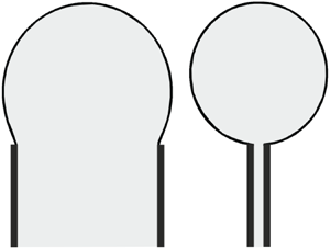
In our previous studies (see Karabut & Zhuravleva Reference Karabut and Zhuravleva2014; Zubarev & Karabut Reference Zubarev and Karabut2018; Karabut et al. Reference Karabut, Zhuravleva and Zubarev2020), we considered problems where the fluid boundary is completely free. Here, we consider a case with a more complicated geometry, where the free boundary is only some part of the entire boundary of the domain occupied by the fluid. The remaining ‘non-free’ part of the boundary is assumed to be an impermeable wall moving in accordance with a specified law. Figures 1(a) and 1(b) illustrate these two variants of boundary conditions by an example of a fluid occupying a bounded domain. The usual no-slip condition is satisfied on such a wall: at each point of the wall, the projections of the wall velocity vector and fluid velocity vector onto the normal to this wall coincide. It is demonstrated in the present paper that such flows, where some part of the boundary is free and some part of the boundary is ‘non-free’, can also be (as in our above-mentioned works) described by a complex Hopf equation. Its solutions can be interpreted as nonlinear perturbations of the base flow with a linear velocity field in the domain bounded by approaching solid walls and a straight-line free boundary (Ovsiannikov Reference Ovsiannikov1967). Note that the problem with walls moving according to a given law has a certain relation to piston and paddle wavemakers, which are widely used in experiments to generate surface water waves; (see, for instance, Sinnis et al. Reference Sinnis, Grare, Lenain and Pizzo2021).

Figure 1. Two variants of boundary conditions. (a) The entire boundary of the fluid is free. The fluid motion occurs by inertia. (b) The fluid boundary consists of the free boundary and a solid wall. The fluid motion occurs both by inertia and under the action of the solid wall.
It should be noted that perturbations of flows with a free boundary are traditionally studied in the linear approximation. This means that, if the exact solution of the problem of motion of the fluid with a free boundary is known in some form, it is possible to consider the stability of this flow with respect to changes in the initial velocity field or initial boundary of the domain. If these changes are small, then the problem of stability can be solved within the framework of the linear theory.
We are not aware of publications that describe an effective method of studying perturbations of an unsteady flow with a free boundary without using an assumption that these perturbations are small. This is not surprising because it is necessary to know not only the flow to be studied, but also a family of flows close to it. Finding such solutions is an extremely complicated task. It turns out that such a problem can be partially solved for flows where the complex velocity satisfies the Hopf equation. For such flows, it is possible to study stability with respect to non-small nonlinear perturbations of the boundary and velocity field (it is assumed that perturbed flows also satisfy the Hopf equation).
The idea of an algorithm for constructing exact solutions of the problem of the dynamics of a fluid with a free surface located between two approaching walls was announced by Zhuravleva et al. (Reference Zhuravleva, Zubarev, Zubareva and Karabut2021). In the present work, in the development of this results, a detailed analysis of the behaviour of singular points of solutions describing the formation of bubbles, cuspidal points and droplets is carried out; without such an analysis it is impossible to assert the existence of solutions. In addition, we demonstrated the possibility of using the developed approach to study flows of fundamentally different topology: as an example, the exact solution describing the collapse of a bubble located in an infinite layer of fluid between two approaching solid walls was constructed and studied. The solutions found have a clear physical meaning; they seem to us important for understanding the basic scenarios for the formation of singularities at free boundaries. They can also be useful for validating numerical codes in the most difficult-to-simulate situations, where an initially smooth free surface becomes singular in a finite time.
2. Formulation of the problem and algorithm for finding solutions
The unknown function to be determined is the complex velocity
 \begin{equation} U(z,t) = u(x,y,t) - \text{i} v(x,y,t). \end{equation}
Here,  $u(x,y,t)$ and
  $v(x,y,t)$ are the projections of the velocity vector onto the
  $x$ and
  $y$ axes (the
  $y$ and
  $x$ axes are directed upward and rightward, respectively).
The function  $U(z, t)$ is an analytical function of the complex variable
  $z = x+ \text {i} y$ because the Cauchy–Riemann conditions are satisfied
 \begin{equation} u_x + v_y = 0, \quad u_y - v_x = 0. \end{equation}
The first equation of (2.2a,b) has the meaning of the condition of fluid incompressibility, and the second one is the condition of flow potentiality.
We seek for the solution in the class of flows described by the Hopf equation (it is also often called the Burgers–Hopf equation)
 \begin{equation} U_t + U U_z = 0. \end{equation}
As was demonstrated previously by Karabut & Zhuravleva (Reference Karabut and Zhuravleva2014), if  $U(z,t)$ satisfies (2.3), then the condition
  $v(x,y,t) = 0$ defines the shape of the free boundary (i.e. the dynamic and kinematic boundary conditions are automatically satisfied on the corresponding curve). The solution of (2.3) within the framework of the method of characteristics is written in the form
 \begin{equation} U(z,t) = G(z - U t), \end{equation}
where the function  $G(z)$ defines the initial complex velocity. Let us rewrite (2.4) via the inverse function
  $F = G^{-1}$. We obtain
 \begin{equation} z = Z(U, t) \equiv U t + F(U). \end{equation}
The solution is sought by the following algorithm.
(i) We specify an arbitrary analytical function
 $F(U)$ satisfying the boundary conditions on the solid walls.
(ii) As
$v=0$ on the free surface, then we find the parametric equation of the free boundary from (2.5)
(2.6a,b)Together with specified laws of motion of the solid walls, this equation defines the flow domain.\begin{equation} x = u t + {{\rm Re}} \,F(u), \quad y = {{\rm Im}}\, F(u). \end{equation}(iii) We verify that the function
$U(z,t)$ defined by (2.4) is holomorphic in the flow domain. The analyticity of this function is violated at those points where the derivative $U_z$ does not exist, which means $Z_U = 0$. It follows from (2.5) that $Z_U = t + F_U(U)$; hence, the singular points are the solutions of the equation
(2.7)Thus, the flow is completely defined by the form of the function\begin{equation} F_U(U) ={-} t. \end{equation}$F(U)$. If we specify two close functions $F_0(U)$ and $F_1(U)$, we obtain two flows close to each other. If we assume that $F_0(U)$ corresponds to the base flow, then $F_1(U)$ can be treated as a certain perturbation of the base flow. In this study, we consider $F_0(U) \equiv 0$ as the base flow. In other words, we consider nonlinear perturbations of the self-similar flow
(2.8)\begin{equation} U = Z/t. \end{equation}


Function (2.8) satisfies the Hopf equation (2.3). Therefore, the free boundary in the plane  $U$ is a straight line
  $v=0$. It is seen from (2.8) that
  $v = -y/t$; therefore, the free boundary in the plane
  $Z$ is a straight line
  $y = 0$. It should be noted that such a flow with a free boundary was constructed for the first time by Dirichlet, who analysed flows with a linear velocity field,
  $U \sim z$. Later on, it was considered, e.g. by Longuet-Higgins (Reference Longuet-Higgins1982), where it was called the ‘upwelling’ flow, which reflects the flow structure at
  $t>0$. It is important that the flow described by (2.8) is consistent with the conditions
  $v=\pm V$ at
  $x = \pm V t$, which corresponds to a situation where the fluid is bounded from the sides by vertical solid walls moving with velocities
  $\pm V$.
Thus, the base flow is assumed to be a two-dimensional plane unsteady flow of an ideal incompressible fluid, where the fluid occupies a semi-infinite strip bounded on the sides by two parallel walls approaching each other with a constant velocity  $V > 0$; the positions of these walls are defined by the equations
  $x = \pm V t$. It is clear from the equation of motion of the walls that they collide at
  $t = 0$. We study the flow before the instant of the collision of the walls, i.e. at
  $t < 0$. The fluid is unbounded from below; at the top, it is bounded by the horizontal free boundary
  $y = 0$. It is easy to find the formula for the streamfunction and demonstrate that the streamlines are hyperbolas. This solution is demonstrated in figure 2. The domain occupied by the fluid is shown by the grey colour. It should be noted that this flow is similar to that found by Ovsiannikov (Reference Ovsiannikov1967) for which the rectangular domain occupied by the medium is compressed by a pair of approaching walls (i.e. the fluid is bounded by two linear segments of the free surface).

Figure 2. Base solution at a certain time instant  $t < 0$.
In the present study, among other results, we consider the nonlinear stability of the flow described above. The presence of an arbitrary function in (2.5) allows us, in fact, to consider non-small disturbances of an almost arbitrary shape for an initially plane free boundary of the fluid. It should be noted that the entire domain of the perturbed flow in the hodograph plane  $(u,-v)$ is constant because the free boundary
  $v = 0$ is fixed, while the solid walls move with constant velocities
  $u = \pm V$. The domain corresponding to the fluid in the hodograph plane is shown in figure 3.

Figure 3. Flow domain in the plane of the complex velocity  $U$.
$U$.
3. Choice of the function $F(U)$

Let us consider the conditions to be satisfied by the function  $F(U)$ in order for the boundary conditions on the solid walls to be valid. On the right wall
  $x = - V t,$ by virtue of the no-slip condition, the horizontal component of the velocity is
  $u = -V$. Substituting it into (2.5), we obtain
  ${{\rm Re}}\, F = 0$. Similarly, for the left wall
  $x = V t,$ where
  $u= V ,$ we obtain
  ${{\rm Re}}\, F = 0$. Thus, the following condition has to be satisfied on the solid walls:
 \begin{equation} {{\rm Re}}\, F|_{u ={\pm} V} = 0. \end{equation}
 In addition to the conditions on the solid walls, the function  $U$ must have no singularities in the flow domain. Therefore, the condition of existence of an inverse function to
  $z(U,t)$ has to be satisfied, namely, the function
  $z(U,t)$ has to be analytical, and its derivative
  $z_U(U,t)$ must have no zeros in the domain occupied by the fluid. As
  $t \in (-\infty, 0)$ in the problem considered here, it is sufficient to require that the real part of the derivative
  $F_U(U)$ should be bounded from above. Then it is possible to find a certain time interval
  $-\infty < t < T < 0$ such that the right-hand side of (2.7) is greater than its left-hand side, which means that there are no singular points in the flow domain at
  $t \in (-\infty, T)$. When these singularities reach the fluid boundary at a certain time instant
  $t_\ast \geq T$, the solution destruction occurs.
According to the known principle of symmetry, if the real part of an analytical function is equal to zero on a certain straight line, then this function can be analytically continued across this straight line. At points symmetric with respect to this straight line, the imaginary parts are identical, while the real parts have identical absolute values, but opposite signs. Thus, we can assume that  $F(U)$ is a
  $2V$-periodic function on the entire domain of its definition. Therefore, we can seek for it in the form of the Fourier series. In view of the boundary conditions (3.1), we have
 \begin{equation} F(U) = \textrm{i} \sum_{n=0}^{\infty} h_n \exp\left(\frac{\textrm{i} {\rm \pi}n (U+V)}{V}\right). \end{equation}
Here,  $h_n$ are complex constants. One of the particular cases of this series is the function
 \begin{equation} F(U) = \frac{\textrm{i} a }{b - \exp(\textrm{i} {\rm \pi}U/V)}. \end{equation}
Let us consider this variant of the perturbation in more detail. It contains three real parameters:  $a, b$ and
  $V$. The parameter
  $V$ is the specified velocity of motion of the solid walls (
 $V > 0$), which also defines the period of the function (3.3). The parameters
  $a$ and
  $b$ define the perturbation shape.
Three points of the free boundary play an important role in the analysis of the free boundary evolution. The first point corresponds to  $x=0$. Two other points, which are points of the free boundary, simultaneously belong to the moving solid walls; they correspond to
  $x = \pm Vt$. The function (3.3) has an interesting property: the ordinates
  $y$ of these three points remain unchanged with time despite the deformation of the free boundary. The ordinate
  $y_0$ of the first point can be easily determined by substituting
  $u = 0$ into the second equation of the free boundary (2.6a,b). We get
 \begin{equation} y_0 = a/(b-1). \end{equation}
The ordinate  $y_{\ast }$ for two other points is obtained by substituting
  $u = \pm V$ into the second equation of (2.6a,b). We have
 \begin{equation} y_{{\ast}} = a/(b+1).\end{equation}
 Under the conditions  $a>0$ and
  $b>1$, (3.4) and (3.5) yield the inequality
 \begin{equation} y_0>y_\ast. \end{equation}
The situation corresponding to inequality (3.6) is illustrated in figure 4(a). This regime can be called the droplet formation regime because not all the fluid is squeezed downward by the approaching solid walls; some part of the fluid remains higher than the level  $y=y_{\ast }$ and forms a droplet.

Figure 4. Variants of non-small perturbations leading to droplet formation (a) and bubble formation (b).
With another choice of parameters, e.g.  $a < 0$ and
  $b < -1$, an alternative flow regime is realized; it is shown in figure 4(b). Here, instead of (3.6), we have the inequality
  $y_0 < y_{\ast }$, and a bubble below the level
  $y=y_{\ast }$ can be formed on the free surface.
Using the fact that the ordinate of the point of contact of the free boundary with the solid wall  $y_{\ast }$ is independent of time, we further assume that the solid walls are bounded from above by
  $y_{\ast }$. Previously, the walls were shown as straight lines parallel to the
  $y$ axis. Now they will be shown as rays parallel to the
  $y$ axis and emanating from the point
  $y_{\ast },$ i.e.
  $-\infty < y \leq y_{\ast }$.
4. Formation of a bubble
Let us first consider a situation corresponding to figure 4(b), i.e.  $a < 0, b < -1$. In this case, a pit is formed on the free surface. Two scenarios are possible depending on the value of the parameter
  $b$: either a bubble or a cusp is formed on the free surface. By virtue of symmetry, when the bubble is formed, i.e. when the free boundaries (2.6a,b) touch each other, the contact point has the abscissa
  $x = 0,$ while the free boundary has a vertical tangent line at this point. Therefore, the contact point satisfies the system of equations
 \begin{equation}
\left. \begin{array}{@{}c@{}} \dfrac{\partial x(u,t)}{\partial u}
= 0, \\
x(u,t) = 0. \end{array} \right\}
\end{equation}
\begin{equation}
\left. \begin{array}{@{}c@{}} \dfrac{\partial x(u,t)}{\partial u}
= 0, \\
x(u,t) = 0. \end{array} \right\}
\end{equation}
We find the real part of the function  $F(u)$ defined by (3.3) and substitute it into the first equation of (2.6a,b). The resultant expression for
  $x$ is substituted into system (4.1). As a result, we have
 \begin{equation}
\left. \begin{array}{@{}c@{}} t = \dfrac{a {\rm \pi}\cos({\rm \pi}
u/V )}{V(1+ b^2 - 2 b \cos({\rm \pi} u/V ) )} - \dfrac{2 a b
{\rm \pi} \sin^2({\rm \pi} u/V )}{V(1+ b^2 - 2 b \cos({\rm \pi} u/V )
)^2}, \\
t u = \dfrac{a \sin({\rm \pi} u/V )}{1+ b^2 - 2 b
\cos({\rm \pi} u/V )}. \end{array} \right\}
\end{equation}
\begin{equation}
\left. \begin{array}{@{}c@{}} t = \dfrac{a {\rm \pi}\cos({\rm \pi}
u/V )}{V(1+ b^2 - 2 b \cos({\rm \pi} u/V ) )} - \dfrac{2 a b
{\rm \pi} \sin^2({\rm \pi} u/V )}{V(1+ b^2 - 2 b \cos({\rm \pi} u/V )
)^2}, \\
t u = \dfrac{a \sin({\rm \pi} u/V )}{1+ b^2 - 2 b
\cos({\rm \pi} u/V )}. \end{array} \right\}
\end{equation}
Eliminating the variable  $t$ from system (4.2), we obtain the equation for
  $u$
$u$
 \begin{equation} (u {\rm \pi}\cos({\rm \pi} u/V ) - V \sin({\rm \pi} u/V ))(1+ b^2 - 2 b \cos({\rm \pi} u/V ) ) - 2 b {\rm \pi}u \sin^2({\rm \pi} u/V ) = 0. \end{equation}
The roots of this equation reveal the position of the point of self-intersection on the free boundary. Obviously, if such a point exists, there exist two symmetric (with respect to the zero point) roots of (4.3). To study (4.3), it is convenient to introduce an additional variable  $\xi ={\rm \pi} u/V$. Let us recall that
  $u \in (-V, V)$ in the general case; therefore, we have
  $\xi \in (-{\rm \pi}, {\rm \pi})$. Let us find the values of the parameter
  $b$ at which the function
 \begin{equation} R(\xi) \equiv (\xi \cos \xi - \sin \xi ) (1+ b^2 - 2 b \cos \xi )- 2 b \xi \sin^2\xi, \end{equation}
has non-zero roots. Using the fact that the function  $R(\xi )$ is odd, we study it on the interval
  $\xi \in (0, {\rm \pi})$. It should be noted that
  $R(0) = 0, R({\rm \pi} ) = - {\rm \pi}(1+b)^2 < 0$; therefore, if
  $R(\xi )$ has a positive maximum point on the interval
  $\xi \in (0, {\rm \pi}),$ it has a root on this interval as well. For this the derivative
 \begin{equation} R'(\xi) ={-} \sin \xi [(1+ b^2) \xi + 4 b \sin \xi], \end{equation}
has to vanish. The first term is always negative at  $\xi \in (0, {\rm \pi})$ and equal to zero at the ends of the interval. Vanishing of the second term means the existence of a point of intersection of the straight line
  $y = (1+ b^2) \xi$ and the sinusoid
  $y = - 4 b \sin \xi$ on the interval
  $\xi \in (0, {\rm \pi})$. Clearly, such a point exists if the slope of the sinusoid at
  $\xi =0$ is greater than the slope of the straight line. We obtain a quadratic inequality for the parameter
  $b$
$b$
 \begin{equation} ( - 4 b \sin \xi )'|_{\xi = 0} ={-}4 b > 1+ b^2. \end{equation}
Solving this inequality with allowance for  $b < -1,$ we obtain
  $-2 - \sqrt {3} < b < -1$. Thus, there exists only one extremum point on the interval
  $\xi \in (0, {\rm \pi})$ at
  $b \in (-2 - \sqrt {3}, \ -1)$. Analysing the signs of
  $R'(\xi )$, we can easily show that this is a maximum point. Therefore, the point of self-intersection of the free boundary appears only at
  $b \in (-2 - \sqrt {3}, \ -1)$. At
  $b \leq -2 - \sqrt {3}$, there are no such points and, hence, the bubble is not formed.
Figure 5 illustrates the evolution of the flow domain at  $a = -1/10, b = -3/2$ and
  $V = 2$. It can be seen that the bubble is formed at the moment
  $\tilde {t}$ when the free boundary self-intersects. A similar situation of solution destruction due to self-intersection of the free boundary, called by the authors the ‘splash’ singularity, was studied by Castro et al. (Reference Castro, Córdoba, Fefferman, Gancedo and Gómez-Serrano2012). A theorem was proved on the existence of such singularities in a finite time interval. In fact, we managed to construct a concrete example of the splash singularity formation. The value of
  $\tilde {t}$ is the result of the numerical solution of system (4.2). For the chosen values of parameters, we have
  $\tilde {t} \approx -0.0462879$. The positions of the singular points of the solution are marked. It is seen that these points are always outside the flow domain, and it is because of self-intersection of the boundary that the solution is destroyed. However, this is not always the case. Let us analyse the behaviour of singular points in more detail.

Figure 5. Formation of a bubble on the free boundary.
5. Analysis of the behaviour of singularities; plane $\mu$

Let us recall that singular points are determined as solutions of (2.7). For type (3.3) of the function  $F(U)$ considered here, (2.7) takes the form
 \begin{equation} \frac{{\rm \pi} a \exp(\text{i} {\rm \pi}U/V)} {V\ (b - \exp(\text{i} U/V))^2} = t. \end{equation}
It is more convenient to continue investigations by introducing an additional notation
 \begin{equation} \mu = \exp(\text{i} {\rm \pi}U/V). \end{equation}
Then (5.1) after several transformations takes the form
 \begin{equation} \mu^2 - \frac{2 V t b + a {\rm \pi}}{V t} \mu + b^2 = 0. \end{equation}
Solving this quadratic equation, we obtain
 \begin{equation} \mu_{1,2} = \frac{a {\rm \pi}+ 2 b t V \pm \sqrt{\rm \pi} \sqrt{a^2 {\rm \pi}+ 4 a b t V}}{2 t V}. \end{equation}
Hence, there are two singular points  $\mu _{1,2}$ in the auxiliary plane
  $\mu$, whose positions are determined by (5.4). Let us denote the time instant when the roots are identical (
 $\mu _1 = \mu _2$) by
 \begin{equation} t_c ={-}\frac{a {\rm \pi}}{4 b V}. \end{equation}
At  $t > t_c$, the roots of the quadratic equation are real. Returning to the replacement (5.2), we find the positions of the singular points in the plane
  $U$ and then, using (2.5), determine the positions of two singularities in the physical plane
  $Z$
$Z$
 \begin{equation}
\left.\begin{array}{@{}c@{}} x = 0,\\ y
= \dfrac{a}{b - |\mu_i|} - \dfrac{V t}{\rm \pi} \ln |\mu_i|,
\quad \mbox{where } i = 1,2. \end{array}\right\}
\end{equation}
\begin{equation}
\left.\begin{array}{@{}c@{}} x = 0,\\ y
= \dfrac{a}{b - |\mu_i|} - \dfrac{V t}{\rm \pi} \ln |\mu_i|,
\quad \mbox{where } i = 1,2. \end{array}\right\}
\end{equation}
Thus, at  $t> t_c$, the singular points move along the
  $y$ axis. Similar formulas can be derived for
  $t< t_c$, when the roots of (5.4) are complex, but these formulas are much more cumbersome.
Figure 6 shows the positions of the free boundary and singular points for some consecutive time instants for  $V= 2, a = -1/10$ and
  $b = -4$. Figure 6(a) corresponds to the time
  $t< t_c$. The singularities are located symmetrically with respect to the
  $y$ axis. They move toward each other and collide at the time instant
  $t= t_c$ shown in figure 6(b). As is further seen from figure 6(c), the singular points again separate and move along the
  $y$ axis; one of them is already visually seen on the free boundary. However, the formation of some singularity in the shape of the free boundary is not observed. Figure 6(d) displays some intermediate situation: one singularity is above the free boundary, and the other one is under the free boundary. Finally, at the time instant illustrated in figure 6(e), the second singular point is seen to reach the free boundary clearly forming a cusp on the boundary. The first singular point is still visualized in the flow domain. As is known, for the solution to exist, the functions should be analytical in the domain occupied by the fluid. Therefore, the following question arises: Is the formation of a cusp on the free boundary really possible or does solution destruction occur earlier, at the time instant shown in figure 6(c)?

Figure 6. Formation of a cusp point on the free boundary.
In our previous studies, we often encountered a situation where the singular point was visually seen to be in the fluid, but it actually was located on another sheet of the Riemann surface. However, in the present study, a direct analysis of the Riemann surface turns out to be rather difficult. For this reason, we propose to consider the auxiliary plane  $\mu$. This variable (5.2) appeared as an additional notation in calculating the singular points of the function.
It can be easily shown that the domain occupied by the fluid in the hodograph plane  $U$ (upper half-strip in figure 7a) is mapped onto the domain in the plane
  $\mu$ in the form shown in figure 7(b). In the plane
  $\mu$, the singular points
  $\mu _1$ and
  $\mu _2$ (5.4) at
  $t< t_c$ are shifted over the arcs of a circumference of radius
  $|b|$ with the centre at the origin until the collision at the point
  $\mu = -b$ at
  $t = t_c$. It should be noted that, once reaching the real axis, the singular points remain on it. One of them moves toward the infinity, and the other one moves toward the origin. Figure 8 shows the positions of two singular points
  $\mu _1$ (red star) and
  $\mu _2$ (blue circle) for different time instants: positions 1–4 correspond to
  $t< t_c$, while positions 6 and 7 correspond to
  $t>t_c$. Position 5 corresponds to merging of the singular points at the time instant
  $t=t_c$. It is clearly seen in this plane that only one singular point reaches the free boundary; see position 7. It can be easily determined from (5.4) that
  $\mu _1 = 1$ at
  $t = t_\ast = a {\rm \pi}/(V(b-1)^2)$ (we always have
  $|t_\ast |<|t_c|$). This means that the singularity
  $\mu _1$ reaches the free boundary at
  $t = t_\ast$. It is this time instant that is shown in figure 6(e); the second singular point reaches the free boundary. Thus, we confirmed the assumption that solution destruction occurs at
  $b < -\sqrt {2} -3$ owing to formation of a cusp on the free boundary.

Figure 7. Mapping of the hodograph plane  $U$ onto the auxiliary plane
  $\mu$.

Figure 8. Motion of singular points in the auxiliary plane  $\mu$.
6. Formation of a droplet
Let us now consider a situation with positive values of the parameters  $a > 0$ and
  $b > 1$ for the flow corresponding to (3.3). In this case,
  $y_0 > y_{\ast }$ (figure 4a), and a droplet is formed on the free surface. Similar to the case with negative parameters, we analyse the positions of singular points. By virtue of periodicity of the logarithmic function of the complex variable, the pair of roots
  $\mu _{1, 2}$ determined by (5.4) at
  $t > t_c$ corresponds to an infinite number of the values of the function
  $U = - \textrm {i} V/{\rm \pi} \ln |\mu _i| + V(1 + 2 n),$ where
  $n$ is integer. In the domain considered here (figure 3), we have
  ${Re}\, U = u \in (-V, V)$; therefore,
  $n$ can take the value of either
  $0$ or
  $-1$. Thus, the motion of singularities in the physical plane at
  $t > t_c$ is described by the system of equations
 \begin{equation}
\left.\begin{array}{@{}c@{}} x = V t (1 + 2 n), \quad n = 0
\mbox{ or } n ={-}1; \\
y = \dfrac{a}{b + |\mu_i|} - \dfrac{V t}{\rm \pi} \ln |\mu_i|. \end{array}\right\}
\end{equation}
\begin{equation}
\left.\begin{array}{@{}c@{}} x = V t (1 + 2 n), \quad n = 0
\mbox{ or } n ={-}1; \\
y = \dfrac{a}{b + |\mu_i|} - \dfrac{V t}{\rm \pi} \ln |\mu_i|. \end{array}\right\}
\end{equation}
Analysing (6.1), we notice that the singularities are always located on vertical straight lines passing through the solid walls. Indeed, if  $n = 0$ in the first equation of system (6.1), then we obtain
  $x = V \, t$, which is the equation of motion of the left solid wall bounding the flow domain; if
  $n = -1,$ then
  $x = -V \, t$, which is the equation of motion of the right solid wall. There are two singular points on each vertical line at
  $t > t_c$. The time instant
  $t = t_c$ is the instant of their separation. Figure 9 shows the shape of the flow domain and the positions of the singular points for some time instants
  $t$ such that
  $t_c \leq t \leq 0$. Some of the singular points are located inside the droplet, i.e. in the domain occupied by the fluid. Let us analyse this situation somewhat later. Now we consider the limiting case
  $t = 0$. The solution has an interesting property: in the limit
  $t \to 0$ (when two plates collide), the free surface takes the shape of a circumference. This can be seen from (2.5) with
  $t = 0$ being assumed; then the equation of the free boundary
  $v=0$ can be written as
 \begin{equation} x+{\rm i}y = F(u) = \frac{{\rm i}a}{b-\exp({\rm i} {\rm \pi}u/V)}. \end{equation}
Identifying the real and imaginary parts, we can easily show that we obtain an equation of a circumference
 \begin{equation} x^2+\left(y-\frac{y_{{\ast}} + y_0}{2}\right)^2=R^2,\quad R=\frac{y_0-y_{{\ast}}}{2}. \end{equation}
Figure 9. Positions of the free boundary and singular points for several time instants  $t_c \leq t \leq 0$.
Figure 9 shows the results of calculations for the fluid boundary shape and positions of singular points performed for  $V=2, b=3/2$ and
  $a=1/10$. The process resembles squeezing of ice cream from a wafer briquette. Let us recall that it is insufficient to find the free boundary position to solve the problem; it is also necessary to prove analyticity of the function of the complex variable inside the flow domain. Figure 9 shows only the free boundary profiles at certain time instants, and we do not argue yet that they correspond to the solution of the fluid flow problem. Below we consider the analyticity of the complex velocity and demonstrate that the solution exists not for all time instants shown in the figure.
The formulas that describe the positions of singular points at  $t < t_c$ are more cumbersome and less informative; therefore, we only provide the calculated positions of the free boundary and singularities for some consecutive time instants
  $t < t_c$. We see in figure 10 that, with increasing
  $t$, the singularities gradually approach the free boundary and change its shape, but still remain outside the flow domain. Therefore, the solution exists at
  $t < t_c$. Let us return to the case with
  $t \geq t_c$ and consider it in more detail.

Figure 10. Positions of the free boundary and singular points for several time instants  $t \leq t_c < 0$.
Figure 11(a) shows the left half of the flow domain and the singular point at the time instant  $t_c$. The solid wall is marked by the dotted line. By enlarging the rectangular area marked in figure 11(a) (figure 11b), we can see that the singular point is located outside the fluid. We know from the analysis of the behaviour of singularities at
  $t > t_c$ that they move along the vertical line
  $x = V t$. Figure 11(c) shows the next time instant
  $t=0.98 t_c$; it is seen that the singular points have separated and move downward; one of them is already on the solid wall, while the other approaches the free boundary.

Figure 11. Behaviour of singular points for the time instants  $t=t_c,\,0.98t_c,\,0.96t_c$ and
  $0.9t_c$.
The time instant  $t=0.96 t_c$ shown in figure 11(d) visually corresponds to the time when the second singular point reaches the free boundary. Finally, it is clearly seen in figure 11(e) (
 $t=0.9t_c$) that one of the singular points is located in the domain occupied by the fluid. It can be assumed that the singular point does not enter the fluid domain in reality; it is located on another sheet of the Riemann surface; for this reason, solution destruction does not occur. An additional study is needed to resolve this issue. The results of such a study are reported below.
7. Analysis of the Riemann surface
Our goal is to find the Riemann surface for the function  $U(z,t)$. In other words, we have to plot the dependence of
  $u$ and
  $v$ on the variables
  $x$ and
  $y$ at a certain time instant
  $t$. However, the corresponding surface can be plotted only in a four-dimensional space; therefore, a projection onto a three-dimensional space is usually used for simplicity. Let us identify the real and imaginary parts in (2.5). As a result, we obtain two real equations
 \begin{equation} x= x(u, v); \quad y = y(u,v). \end{equation}
Eliminating  $u$ from system (7.1a,b), we obtain the equation
 \begin{equation} v = h(x, y), \end{equation}
which describes the Riemann surface in a three-dimensional space  $x, y, v$. With such an approach, it is convenient to construct the free boundary, resulting from intersection of the surface (7.2) by the plane
  $v = 0$. The analysis of the Riemann surface allows us to determine whether the singularities and the domain occupied by the fluid are located on one sheet of the Riemann surface.
Let us consider the cross-section of the surface (7.2) by the plane  $x = V t$ corresponding to the left wall. Substituting
  $x = V t,\ u = V$ and
  $F(U),$ defined by (3.3), into (2.5), we obtain an equation for implicit definition of the function
  $v (y,t)$
 \begin{equation} y + v t - \frac{a}{b + {\rm e}^{{\rm \pi} v/V}} = 0. \end{equation}
Figure 12 shows the dependence of  $v$ on
  $y$ for several time instants:
  $t = 1.5 t_c \approx -0.04$,
  $t = 0.96 t_c = t_{\ast } \approx -0.025$ and
  $t = 0.8 t_c \approx -0.02$. The curves were obtained for the following values of parameters:
  $b = 3/2, a = 1/10$ and
  $V = 2$. The vertical tangent line is shown by the dotted curve. At the time instant
  $t = t_{\ast }$, there appears a vertical tangent line of the function
  $v(y)$ at
  $v=0$ (
 $v=0$ is the equation of the free boundary). This time instant exists for any positive
  $b$; it can be calculated analytically. For this purpose, we consider the implicitly defined function
  $v(y)$ in the form
 \begin{equation} G(y,v,t) \equiv y + v t - \frac{a}{b + {\rm e}^{{\rm \pi} v/V}} = 0, \end{equation}
and calculate  $v_y'$ for this function
 \begin{equation} \frac{{\rm d} G}{{\rm d} y} = \frac{\partial G}{\partial y} + \frac{\partial G}{\partial v} \cdot \frac{\partial v}{\partial y} = 0 \Rightarrow \frac{\partial v}{\partial y} ={-} \frac{G_y'}{G_v'}. \end{equation}
Therefore, for the plot of the function to have a vertical tangent line, it should be  $G'_v = 0$. Let us calculate this derivative and equate it to zero on the free boundary, i.e. at
  $v = 0$
 \begin{equation} G_v'|_{v=0}=t+\frac{a \,{\rm e}^{{\rm \pi} v/V}\cdot {\rm \pi}/V}{(b+ {\rm e}^{{\rm \pi} v/ V})^2}|_{v=0}=0 \Rightarrow t+\frac{a{\rm \pi}}{V(b+1)^2}=0 \Rightarrow t_\ast{=}{-}\frac{a{\rm \pi}}{V(b+1)^2}. \end{equation}
It should be noted that the value  $t = t_{\ast }$ coincides with the previously calculated time instant when the singular point reaches the free boundary, see figure 11(d) (
 $|t_{\ast }|<|t_c|$ always). In our opinion, the many valuedness of the function
  $v(y, t)$ at
  $t > t_{\ast }$ (see figure 12) testifies to solution destruction associated with reaching the free boundary by the singular point.

Figure 12. Cross-sections of the Riemann surface for some time instants.
Thus, solution destruction occurs earlier than the walls collide at  $t=0$, namely, at the time instant
  $t_{\ast }<0$ when the singularity passes from the domain outside the flow to the contact point of the free boundary and moving wall. Figure 13 demonstrates the final (those that refer to the time instant
  $t_{\ast }$) shapes of the fluid boundary for different values of
  $b$. Here, we take
  $a=b^{2}-1$, which ensures an unchanged (equal to 2) difference in the fluid height on the free surface
  $(y_0-y_\ast )$ with variation of the parameter
  $b$. As
  $b$ decreases, the tendency to droplet formation becomes more pronounced. The width of its neck
  $d$ is determined from the positions of the walls at the time
  $t_\ast$, i.e. is defined by the formula
  $d=-2Vt_\ast =2{\rm \pi} a/(1+b)^{2}$. In the limit
  $b\to 1$ at
  $a=b^{2}-1$, we obtain a circular droplet with a unit radius, while the neck width
  $d\approx {\rm \pi}(b-1)$ tends to zero.

Figure 13. Final (those that refer to the solution breakdown times  $t_\ast$) shapes of the domain occupied by the fluid for different values of
  $b$,
$b$,  $a=b^{2}-1$ and
  $V=2$.
8. Collapse of a bubble
Let us consider one more variant of the function  $F(U)$ providing a principally different flow topology as compared with the examples considered above
 \begin{equation} F(U) ={-}\frac{R}{b} \arcsin \sqrt{\frac{\sin^2({\rm \pi} U/2 V)-a}{1-a}}, \quad \mbox{where} \ b = \textrm{arsinh} \sqrt{\frac{a}{1-a}}. \end{equation}
Here,  $V > 0$ is the wall motion velocity, as previously;
  $0 < a < 1$ and
  $R >0$ are the parameters characterizing the bubble shape and size. To avoid many valuedness of the function of the square root, we choose its branch that converts the point
  $U =0$ in the hodograph plane after the mapping
  $Z = U t + F(U)$ to the point
  $Z = - \textrm {i} R$ in the physical plane.
It should be noted that this problem can be interpreted as one more variant of the non-small perturbation  $F(U)$ superimposed onto the self-similar flow
  $U = Z/t$; however, it can be also considered as an independent exact solution that describes a collapse of a bubble located in the fluid between two parallel solid walls approaching each other with a constant velocity
  $V$. Looking ahead, we can note that the collapse occurs at the time instant
  $t=0,$ while the walls collide later, at the time instant
 \begin{equation} t = t_0 \equiv \frac{{\rm \pi} R}{2 bV}>0. \end{equation}
We assume that the flow under study is symmetric with respect to the  $x$ and
  $y$ axes; therefore, it is sufficient to study the problem in the domain
  $x<0, y<0,$ which corresponds to the half-strip
  $0< u< V, v<0,$ in the hodograph plane, see figure 14(a). First, we verify that definition of
  $F(U)$ by (8.1) is consistent with the no-slip condition on the moving solid wall, i.e. its velocity coincides with the normal component of the fluid velocity. Let us see what happens to the wall
  $u = V$ after the mapping
  $Z = U t + F(U)$. For this purpose, we calculate
  $F(V - \textrm {i} v)$
 \begin{align} F(V -
\textrm{i} v) &={-} \frac{R}{b} \arcsin
\sqrt{\frac{\sin^2\left(\dfrac{\rm \pi}{2} - \textrm{i}
\dfrac{{\rm \pi} v}{2 V}\right) - a}{1-a}} ={-} \frac{R}{b}
\arcsin \sqrt{\frac{\textrm{cosh}^2\left(\dfrac{{\rm \pi} v }{2
V}\right) - a}{1-a}} \nonumber\\
&={-} \frac{{\rm \pi} R}{2 b} + \textrm{i} \frac{R}{b} \ln
\left(\sqrt{\frac{\textrm{cosh}^2\dfrac{{\rm \pi} v }{2 V} -
a}{1-a}} + \sqrt{\frac{\textrm{cosh}^2\dfrac{{\rm \pi} v }{2 V}
- 1}{1-a}} \right).
\end{align}
\begin{align} F(V -
\textrm{i} v) &={-} \frac{R}{b} \arcsin
\sqrt{\frac{\sin^2\left(\dfrac{\rm \pi}{2} - \textrm{i}
\dfrac{{\rm \pi} v}{2 V}\right) - a}{1-a}} ={-} \frac{R}{b}
\arcsin \sqrt{\frac{\textrm{cosh}^2\left(\dfrac{{\rm \pi} v }{2
V}\right) - a}{1-a}} \nonumber\\
&={-} \frac{{\rm \pi} R}{2 b} + \textrm{i} \frac{R}{b} \ln
\left(\sqrt{\frac{\textrm{cosh}^2\dfrac{{\rm \pi} v }{2 V} -
a}{1-a}} + \sqrt{\frac{\textrm{cosh}^2\dfrac{{\rm \pi} v }{2 V}
- 1}{1-a}} \right).
\end{align}
As  $0< a<1$, the expression in the argument of the logarithm (8.3) is a positive real number. Substituting (8.3) into (2.5) and assuming that
  $u = V,$ we obtain
 \begin{equation} x = V t + {{\rm Re}}\, [F(V - \textrm{i }v)] = V t - \frac{{\rm \pi} R}{2 b} = V \left( t - \frac{{\rm \pi} R}{2 b V}\right). \end{equation}
Therefore, the motion of the solid wall in the physical plane is described by the equation
 \begin{equation} x = (t-t_0)V. \end{equation}
We assume that  $t< t_0,$ so that the wall moves toward the
  $y$ axis and reaches it at the time instant
  $t_0$. Expression (8.5) differs from that used in the previous paragraphs by a time shift by
  $t_0$.

Figure 14. (a) Part of the hodograph plane under consideration. (b) Mapping onto the auxiliary plane  $\mu$.
The free boundary  $v = 0$ is defined in the physical plane by the parametric equations (2.6a,b) where
  $u \in (0, \ V)$. Together with the equation of solid wall motion (8.5), these equations describe the domain occupied by the fluid. It is shown in figure 15 at
  $t = -t_0/2$ for
  $a = 1/2, V = 1$ and
  $R = 1$. The line ABC corresponds to the free boundary, and it is seen that the free boundary is not smooth. It consists of a curvilinear segment AB and a straight-line segment BC, which meet at the point B. It is seen that there is a singularity at this point (corner): the boundary turns at this point by
  ${\rm \pi} /2$. The presence of the singular point
  ${\rm B}$ is inherent in the structure of the function
  $F(U)$. Indeed, let us find the points where the function is not differentiable. Its derivative is defined by the expression
 \begin{equation} F_U={-}\frac{t_0 \sin \left(\dfrac{{\rm \pi} U}{2 V}\right)}{\sqrt{\sin^2 \left(\dfrac{{\rm \pi} U}{2 V}\right)-a}}. \end{equation}
It turns to infinity when the denominator turns to zero. As previously (see (5.2)), the analysis is performed in terms of the auxiliary variable  $\mu = \textrm {e}^{\textrm {i} {\rm \pi}U/V}$. This mapping converts the flow domain in the hodograph plane (half-strip
  $0< u < 1$,
  $v <0$, see figure 14a) to the upper half of a unit circle with the centre at the origin, see figure 14(b). The position of the point B in figure 14 corresponds to
  $a=1/2$.

Figure 15. Domain occupied by the fluid in the quadrant  $x<0$ and
  $y<0$ at the time instant
  $t = -t_0/2$.
Two singularities arising due to vanishing of the denominator in (8.6) have the form
 \begin{equation} \mu_{1, 2} = 1- 2 a \pm 2 \textrm{i} \sqrt{a (1-a)}. \end{equation}
One of them,  $\mu _2$, has a negative imaginary part; therefore, it is located outside the flow domain. The absolute value of the second singularity is
  $|\mu _1| = 1$, therefore, it is a stationary point in the plane
  $\mu$, which is always located on the free boundary. It should be noted that the singular point on the free boundary does not contradict the existence of the solution because the function remains analytical inside the flow domain. In the physical plane, the location of the singular point on the free boundary leads to the loss of smoothness and to the emergence of a corner of
  ${\rm \pi} /2$ on the free boundary (see figure 15).
Let us consider now whether the condition that the complex velocity function for the chosen function  $F(U)$ should be holomorphic in the flow domain is satisfied. The singular points are defined as solutions of (2.7), which takes the following form for (8.1):
 \begin{equation} t_0 \sin \left(\frac{{\rm \pi} U}{2 V}\right) = t\ \sqrt{\sin^2 \left(\frac{{\rm \pi} U}{2 V}\right)-a}. \end{equation}
Raising both sides of (8.8) to the second power and replacing the variables  $U\to \mu$, we obtain the quadratic equation
 \begin{equation} (t_0^2 - t^2) \mu^2 + 2 (t^2 (1- 2a) - t_0^2) \mu + (t_0^2 - t^2) = 0. \end{equation}
We are interested in the evolution of the solution at times close to the collapse instant  $t = 0$, and we can choose an arbitrary value of
  $t$ as the initial time instant. We choose the interval
  $-t_0 < t < 0$ on which the higher coefficient of (8.9) retains its sign. On this interval, (8.9) has two real roots
 \begin{equation} \mu_{3, 4} = \frac{t_0^2 + (2 a -1) t^2 \pm 2 t \sqrt{a (t_0^2 - (1-a) t^2)}}{ t_0^2 - t^2}, \end{equation}
for which
 \begin{equation} \lim_{t \rightarrow - t_0 +0} \mu_{3} = 0, \quad \lim_{t \rightarrow - t_0 +0} \mu_{4} ={+} \infty, \quad \lim_{t \rightarrow 0} \mu_{3} = \lim_{t \rightarrow 0} \mu_{4} = 1. \end{equation}
Thus, at  $t \in (-t_0, \ 0)$, the singular point
  $\mu _{3}$ runs over a segment of the real axis from the point D to the point A (see figure 14b), while the point
  $\mu _{4}$ moves outside the flow domain over the real axis and approaches point A from the outer side of the circle. It should be noted, however, that the points
  $\mu _{3,\ 4}$ found here are roots of the equation corollary obtained by raising the initial (8.8) to the second power. Let us demonstrate that
  $\mu _3$ is not a root of the initial equation. For this purpose, we return to the variable
  $U$. As
  $\mu _3 \in {\rm R}$ and
  $\mu _3 > 0,$ then
  $\ln \mu _3 = \ln |\mu _3|$. We have
 \begin{align} \mu = {\rm e}^{\textrm{i} {\rm \pi}U/V} &\Rightarrow U ={-} \textrm{i} \frac{V}{\rm \pi} \ln |\mu_3| \Rightarrow \sin \frac{{\rm \pi} U}{2 V} ={-} \textrm{i} \,\textrm{sinh} \left(\frac{ \ln |\mu_3| }{2} \right)\nonumber\\ &\Rightarrow \sqrt{\sin^2 \frac{{\rm \pi} U}{2 V} - a} = \textrm{i} \sqrt{\textrm{sinh}^2 \left(\frac{ \ln |\mu_3| }{2} \right) + a}. \end{align}
Substituting the resultant expression into the initial equation (8.8), we find
 \begin{equation} - t_0\ \textrm{sinh} (\ln |\mu_3| /2 ) = t \sqrt{\textrm{sinh}^2 (\ln |\mu_3|/2 ) + a}. \end{equation}
However, the equality is invalid because  $\mu _3 < 1$ and, therefore, the left-hand side of (8.13) is positive, whereas the right-hand side is negative. Therefore,
  $\mu _3$ is not a root of (8.8), and its position in the flow domain does not violate the analyticity of the complex velocity function.
Thus, we proved the existence of the solution at  $t\in (-t_0,\ 0)$. Let us now use the property of symmetry and continue this solution (figure 15) across the
  $x$ and
  $y$ axes. As a result, we obtain a flow that can be treated as a collapse of the bubble located in the fluid between two parallel walls moving toward each other with a constant velocity. Figure 16 shows the evolution of this flow for the following values of the parameters:
  $R = 1, V = 1$ and
  $a = 1/2$. The positions of the singularities are marked. One of them marked by the circle corresponds to the root
  $\mu _1$, and the other one marked by the star corresponds to the root
  $\mu _4$.

Figure 16. Evolution of a bubble.
At  $t = 0$, the bubble completely collapses to a segment
  $[-R, R]$ located on the imaginary axis. This occurs at the time instant when the singularity
  $\mu _4$ passes from the domain outside the fluid to the free boundary, which is accompanied by the formation of a singularity, i.e. a point with an infinite curvature corresponding to the end of the segment.
9. Conclusions
A number of new exact solutions of the classical problem of the hydrodynamics on a plane unsteady potential flow of an ideal incompressible fluid with a free boundary are constructed and studied. In our earlier investigations (see Karabut & Zhuravleva Reference Karabut and Zhuravleva2014; Zubarev & Karabut Reference Zubarev and Karabut2018; Karabut et al. Reference Karabut, Zhuravleva and Zubarev2020), we considered a situation where the entire boundary of the fluid is free. For this case, an algorithm for constructing exact solutions was proposed for situations where the domain corresponding to the fluid does not change with time in the plane of the complex velocity  $U$ (hodograph plane). The solution
  $z(U,t)$ is found by the compact formula
 \begin{equation} z=Ut+F(U), \end{equation}
where  $F(U)$ is a sufficiently arbitrary function holomorphic in the flow domain.
It is demonstrated in the present paper that presentation (9.1) remains valid if some of the fluid boundaries are solid walls moving with a constant velocity. In this case, the function  $F(U)$ has to satisfy additional boundary conditions on the walls. Note that some solutions, such as those shown in figures 5 and 6, allow analytical continuation beyond the solid walls. In this case, we obtain rather exotic periodic solutions of the problem for a purely free surface flow; the spatial period
  $|2 V t|$ of boundary perturbations changes linearly with time.
Dividing the function  $F(U)$ into a pair of functions,
  $F(U)=F_0(U)+F_1(U)$, (9.1) can be considered as a solution that describes a perturbation of a certain base flow
  $z=Ut+F_0(U)$. In this case, the perturbations are defined by the function
  $F_1(U)$. As our approach does not require that
  $F$ should be small and, as a consequence that
  $F_0$ and
  $F_1$ should be small, it actually offers new possibilities of studying the stability of unsteady flows with a free boundary to non-small nonlinear perturbations.
It is clear from general considerations that the complete solution of the problem under consideration has to contain a pair of arbitrary functions: one of them is responsible for the initial shape of the free boundary, and the other is responsible for the initial velocity perturbation. A solution of the form of (9.1) is a particular solution because it contains only one arbitrary function  $F$. As a result, it is possible to specify an arbitrary shape of the boundary, but the velocity field is not arbitrary; it is defined by relation (9.1). A specific feature of the class of solutions described by (9.1) is the absence of the vertical component of velocity on the free boundary, which certainly imposes significant constraints on the types of flows described by our approach, and thus leaves the possibility of a qualitatively different behaviour for a more general class of perturbations. However, the presence of even one arbitrary function can be considered as a noticeable achievement. As was shown by several examples, our solutions allow one to describe various important processes, such as the formation and collapse of bubbles and the formation of droplets and cusps. The question about the possibility of complete integration of equations of motion is still open. Probably, the general solution being presented in the form
 \begin{equation} z=Ut+\tilde{F}(U,t), \end{equation}
can be constructed in the form of a formal series as an expansion of the function  $\tilde {F}(U,t)$ in powers of
  $t$, where the function
  $F(U)$ included in (9.1) plays the role of the zeroth approximation. For a fluid not bounded by walls, the possibility of implementation of an iterative procedure for constructing the general solution was discussed by Zakharov (Reference Zakharov2020). In that case, an approach based on conformal mapping of the domain occupied by the fluid onto a half-plane was applied (see Dyachenko et al. Reference Dyachenko, Kuznetsov, Spector and Zakharov1996; Dyachenko Reference Dyachenko2001), which differs from the hodograph transform used in our study. It should be noted that integrability is supported by the presence of new integrals of motion arising in the course of integration around singularities located outside the fluid, which was noted in Dyachenko et al. (Reference Dyachenko, Dyachenko, Lushnikov and Zakharov2019, § 1). The theory here is based on assumptions about a certain behaviour of the singularities and their type (see also the recent publication Lushnikov & Zakharov Reference Lushnikov and Zakharov2021). The validity of the assumptions and results (Dyachenko et al. Reference Dyachenko, Dyachenko, Lushnikov and Zakharov2019) can be verified through comparisons with solutions derived in the present study.
Funding
This research received no specific grant from any funding agency, commercial or not-for-profit sectors.
Declaration of interests
The authors report no conflict of interest.


