2.1. Immersed boundary method

We carry out the direct numerical simulation (DNS) of a three-dimensional uniform flow past a flapping plate with the free-stream velocity $U$. The zero-thickness plate heaves vertically and pitches around the centre of the plate. The plate has the chord length $c$ and fixed wing span $b=R_A c$, where $R_A$ is the aspect ratio. Figure 1(a) sketches the flapping plate and the Cartesian coordinate system with the $x$-axis along the streamwise direction, the $y$-axis along the spanwise direction and the $z$-axis along the vertical direction. The kinematics of the flapping plate is characterized by the angle of attack

(2.1)\begin{equation} \alpha(t)=\alpha_{0}+\alpha_{m} \cos (2 {\rm \pi}f t) ,\end{equation}

and the vertical position of the plate centre

(2.2)\begin{equation} z_{c}(t)=z_{c 0}+A \sin (2{\rm \pi} f t), \end{equation}

where $\alpha _m$ and $A$ respectively denote the pitching and heaving amplitudes, $\alpha _0$ and $z_{c0}$ respectively denote the time-averaged $\alpha$ and $z_c$, $f$ is the flapping frequency and $t$ is the physical time. All the variable and parameters in the present study are non-dimensionalized by $U$ and $c$.

Figure 1. Schematic diagrams of the coordinate system and local-refined mesh. (a) Flow past a flapping plate with the coordinate system $O$-$xyz$. (b) Flow-field domain $\varOmega$ and VSF domain $\varOmega _{\phi }$ on the $x$–$z$ plane at $y=0$. The white line denotes the plate, and the $x$-coordinate denotes the streamwise position non-dimensionalized by the chord length.

Motivated by the numerical simulations (Dong et al. Reference Dong, Mittal and Najjar2006; Li & Lu Reference Li and Lu2012; Wang et al. Reference Wang, Zhang, He and Liu2013; Li & Dong Reference Li and Dong2016) and experiments (Buchholz & Smits Reference Buchholz and Smits2006, Reference Buchholz and Smits2008) of low-aspect-ratio flapping wings, we conduct a series of DNS cases with the varying parameters listed in table 1. Here, $Re=Uc/\nu$ is the Reynolds number with the kinematic viscosity $\nu$, and $St = 2Af/U$ is the Strouhal number. Case 1 with $St=0.6$ is mainly used to study of the VSF evolution and force modelling. This case has a discrete wake dominated by two sets of isolated vortical structures, similar to the wake topology observed in Dong et al. (Reference Dong, Mittal and Najjar2006), Li & Lu (Reference Li and Lu2012), Li & Dong (Reference Li and Dong2016) and Li et al. (Reference Li, Dong and Liang2016). Furthermore, the wake can be more convoluted with the increase of $Re$, $St$ or $R_A$ (Dong et al. Reference Dong, Mittal and Najjar2006; Wang et al. Reference Wang, Zhang, He and Liu2013; Liu, Dong & Li Reference Liu, Dong and Li2016).

Table 1. Parameters for the flapping plate in the DNS.

The incompressible flow past a flapping plate is governed by the Navier–Stokes equations

(2.3)$$\begin{gather} \frac{\partial \boldsymbol{u}}{\partial t}+\boldsymbol{u} \boldsymbol{\cdot} \boldsymbol{\nabla} \boldsymbol{u}={-}\boldsymbol{\nabla} p+\frac{1}{R e} \nabla^{2} \boldsymbol{u}+\boldsymbol{f}, \end{gather}$$

(2.4)$$\begin{gather}\boldsymbol{\nabla} \boldsymbol{\cdot} \boldsymbol{u}=0, \end{gather}$$

where $\boldsymbol {u}$, $p$ and $\boldsymbol {f}$ denote the non-dimensional velocity, pressure and body force, respectively. We use the immersed boundary method with the discrete streamfunction (Wang & Zhang Reference Wang and Zhang2011) to solve (2.3) and (2.4). The geometry and kinematics of the plate are described by Lagrangian marker points uniformly distributed on the immersed boundary. The interpolation and spreading of forces on Eulerian and Lagrangian points are linked by the regularized delta function $\delta _h$ (Peskin Reference Peskin2002) as

(2.5)\begin{equation} \sum_{j=1}^{M}\left(\sum_{\boldsymbol{x}} \delta_{h}(\boldsymbol{x}-\boldsymbol{X}_{j}) \delta_{h}(\boldsymbol{x}-\boldsymbol{X}_{k})(\Delta s)^{2}(\Delta x )^{3}\right) \boldsymbol{F}(\boldsymbol{X}_{j}) =\frac{\boldsymbol{U}_b(\boldsymbol{X}_{k})-\boldsymbol{U}^{*}(\boldsymbol{X}_{k})}{\Delta t} , \end{equation}

and

(2.6)\begin{equation} \boldsymbol{f}(x)=\sum_{j=1}^{M} \boldsymbol{F}(\boldsymbol{X}_{j}) \delta_{h}(\boldsymbol{x}-\boldsymbol{X}_{j})(\Delta s)^{2}, \end{equation}

where $\boldsymbol {x}$ and $\boldsymbol {X}$ are Eulerian and Lagrangian points, respectively, $\boldsymbol {f}$ and $\boldsymbol {F}$ are the forces on Eulerian and Lagrangian points, respectively, $\Delta s$ and $\Delta x$ are Lagrangian and Eulerian grid spacings, respectively, $\boldsymbol {U}_b$ and $\boldsymbol {U}^*$ are specified and predicted velocities at $k$th Lagrangian points, respectively, and $M$ is the total number of Lagrangian points on the immersed boundary. The details and validation of our implementation of the immersed boundary method can be found in Wang & Zhang (Reference Wang and Zhang2011) and Wang et al. (Reference Wang, Zhang, He and Liu2013).

The thrust coefficient of the flapping plate is

(2.7)\begin{equation} C_{T}=\frac{F_T}{\frac{1}{2} \rho U^{2} R_{A}c^2}, \end{equation}

where $F_T$ is the thrust of the flapping plate. From the DNS data, it is calculated by

(2.8)\begin{equation} C_{T}={-}\frac{\displaystyle\sum_{k=1}^{M} F_{x}(\boldsymbol{X}_{k})(\Delta s)^{2}}{\frac{1}{2} \rho U^{2} R_{A}c^2}, \end{equation}

where $F_x$ denotes the $x$-component of the force on Lagrangian points.

As shown in figure 1(b), the present simulation is performed in a rectangular domain of $\varOmega \in [-14,22]\times [-18,18]\times [-18,18]$. The uniform inflow velocity $U$ is prescribed at the inlet and the fixed pressure condition is specified at the outlet. The slip-wall condition is used at the other four boundaries and the no-slip condition is specified on the plate. The initial condition for the flow is $\boldsymbol {u}=(U,0,0)$. A locally refined mesh with the minimum spacing $\Delta x=0.0125$ is applied around the immersed boundary to achieve the high spatial resolution near the plate, and the maximum spacing $\Delta x=0.4$ is applied in the far field to reduce the computational cost. The total number of grid points is $12$ million. The effectiveness of the present mesh spacing and computational domain has been validated by a convergence test via varying the grid size and computational domain in Appendix A.

2.2. VSF method

The VSF is a smooth scalar field satisfying the constraint (see Yang & Pullin Reference Yang and Pullin2010)

(2.9)\begin{equation} \boldsymbol{\omega} \boldsymbol{\cdot} \boldsymbol{\nabla} \phi_v=0, \end{equation}

where $\boldsymbol {\omega }=\boldsymbol {\nabla } \times \boldsymbol {u}$ is the vorticity, so that the isosurface of $\phi _v$ is a vortex surface consisting of vortex lines. Given a time series of the velocity–vorticity field obtained by solving (2.3) and (2.4), the calculation of the VSF can be implemented as a postprocessing step.

The two-time method (Yang & Pullin Reference Yang and Pullin2011) with source terms exerted on the immersed boundary (Tong et al. Reference Tong, Yang and Wang2020) is used for calculating the temporal evolution of VSF. For each physical time step, it involves prediction and correction substeps. In the prediction substep, the temporary VSF solution is advanced in the physical time as

(2.10)\begin{equation} \frac{\partial \phi_{v}^{*}(\boldsymbol{x}, t)}{\partial t}+\boldsymbol{u}(\boldsymbol{x}, t) \boldsymbol{\cdot} \boldsymbol{\nabla} \phi_{v}^{*}(\boldsymbol{x}, t)=q(\boldsymbol{x}),\quad t \geq 0, \end{equation}

where $\phi _{v}^{*}$ is a temporary VSF solution which can be deviated from the accurate VSF. In the correction substep, $\phi _{v}^{*}$ is transported along the frozen vorticity as

(2.11)\begin{equation} \frac{\partial \phi_{v}(\boldsymbol{x}, t ; \tau)}{\partial \tau}+\boldsymbol{\omega}(\boldsymbol{x}, t) \boldsymbol{\cdot} \boldsymbol{\nabla} \phi_{v}(\boldsymbol{x}, t ; \tau)=q_{\tau}(\boldsymbol{x}), \quad 0 \leq \tau \leq T_{\tau}, \end{equation}

with

(2.12)\begin{equation} \phi_{v}(\boldsymbol{x}, t; \tau=0)=\phi_{v}^{*}(\boldsymbol{x}, t). \end{equation}

In (2.10) and (2.11), the external VSF source terms $q(\boldsymbol {x})$ and $q_{\tau }(\boldsymbol {x})$ defined on Eulerian grid points are used to satisfy $\phi _v=\phi _v^{B}$ at the immersed boundary, with constant $\phi _v^B=1$ on the plate. Finally, $\phi _v$ is updated by $\phi _{v}(\boldsymbol {x}, t ; \tau =T_{\tau })$ after the pseudo-time evolution, where $T_{\tau }$ is the maximum pseudo-time to ensure the convergence of $\phi _v$ in (2.11), and it is typically less than 100 times of $\Delta t$ in (2.10).

As shown in figure 1(b), the VSF calculation is implemented in a subdomain $\varOmega _{\phi } \in [-1.0, 7.5] \times [-1.5, 1,5] \times [-3.5, 3.5]$ around the plate and near wake with strong vorticity. In $\varOmega _{\phi }$, the high-resolution uniform mesh with $\Delta x=0.02$ is set to ensure the smoothness of numerical VSF solutions. The velocity and vorticity fields in $\varOmega _{\phi }$ are interpolated from $\varOmega$ through the quadratic Shepard method (Franke Reference Franke1982).

To solve (2.10) and (2.11), the marching of $t$ and $\tau$ is approximated by the second-order total-variation-diminishing Runge–Kutta method, and the convection term is calculated by the fifth-order weighted essentially non-oscillatory (WENO) scheme. The numerical diffusion in the WENO scheme serves as the numerical dissipation regularization for smoothing VSFs.

An initial VSF $\phi _{v0}$ needs to be specified to solve (2.10). The initial set-up implies that $\boldsymbol {\omega }=0$ at $t=0$, and $\boldsymbol {\omega }$ is generated at $t>0$. Since the vorticity is dominated on the spanwise direction and $|\boldsymbol {\omega }|$ is close to an exact VSF at very early times (see Tong et al. Reference Tong, Yang and Wang2020), we use $|\boldsymbol {\omega }|$ at $t=t_0=0.02$ to set

(2.13)\begin{equation} \phi_{v 0}(\boldsymbol{x}, t_{0} ; \tau=0)=\sqrt{\frac{|\boldsymbol{\omega}(\boldsymbol{x})|}{|\boldsymbol{\omega}(\boldsymbol{x})|_{max}}}, \end{equation}

and then the initial VSF

(2.14)\begin{equation} \phi_{v 0}=\phi_{v 0}(\boldsymbol{x}, t_{0} ; \tau=T_{\tau}) \end{equation}

at $t=t_0$ is obtained by solving (2.11), where $|\boldsymbol {\omega }(\boldsymbol {x})|_{max}$ denotes the maximum of $|\boldsymbol {\omega }(\boldsymbol {x})|$ in $\varOmega _\phi$.

We remark that the numerical dissipation in the VSF convection can cause the artificial decay of the numerical VSF solution, so we compensate the numerical VSF before each physical time step in the two-time method based on the volume-averaged VSF $\langle \phi _{v0}\rangle$ and local $|\boldsymbol {\omega }|$. Since $\phi _v$ decays along with $x$, we empirically augment the VSF solution downstream as

(2.15)\begin{equation} \phi_v(\boldsymbol{x},t) = \tilde{\phi}_v(\boldsymbol{x},t) \gamma^{{(\alpha_l|\boldsymbol{\omega}(\boldsymbol{x})|)}/{|\boldsymbol{\omega}(\boldsymbol{x})|_{max}}}, \end{equation}

where $\tilde {\phi }_v$ denotes an intermediate VSF solution before the augmentation, $\gamma =\langle \phi _{v0}\rangle /\langle \tilde {\phi }_{v}(\boldsymbol {x},t)\rangle > 1$ is an augmentation factor and $\alpha _l = l_x/(l_x+x^3)$ is an empirical parameter with the streamwise length $l_x$ of $\varOmega _{\phi }$. From numerical experiments, we find that this augmentation can effectively reduce the VSF dissipation or the volume shrinking of a particular VSF isosurface in the present simulation.

Starting from the constructed $\phi _{v0}$, the numerical VSF solution is calculated by solving (2.10) and (2.11) with (2.15). The deviation of the numerical VSF from the exact VSF is monitored by the cosine of angle between the vorticity and VSF gradient as

(2.16)\begin{equation} \lambda_{\boldsymbol{\omega}} \equiv \frac{\boldsymbol{\omega} \boldsymbol{\cdot} \boldsymbol{\nabla} \phi_{v}}{|\boldsymbol{\omega}||\boldsymbol{\nabla} \phi_{v}|}. \end{equation}

We find that the volumed-averaged VSF deviation $\langle |\lambda _{\boldsymbol {\omega }}| \rangle$ over $\varOmega _\phi$ is controlled to within approximately $4\,\%$, indicating that the VSF solution is sufficiently accurate for the further characterization of vortex surfaces and modelling of forces.

3.1. Formation of ring-like vortex surfaces

At the initial time, the plate is located at $z_c=0$ with the maximum angle of attack $\alpha =30^{\circ }$. The plate heaves upwards to the highest point at $t=T/4$ by (2.2). In the meantime, the positive $\alpha$ decreases to $0\,^{\circ }$ during this quarter cycle by (2.1). As shown in figure 2(a), the bulge-like vortex surface $V_1$ with counterclockwise vortex lines from the top view is generated around the tip and the trailing edge of the plate. The VSF isosurface is color-coded by $|\boldsymbol {\omega }|$, and in general $\phi _v$ is positively correlated to $|\boldsymbol {\omega }|$.

Figure 2. Temporal evolution of VSF isosurfaces during the downstroke. Left column: the red solid line denotes the plate at the present time and the red dashed line shows the previous location of the plate. Right column: the VSF isosurfaces are colour coded by the vorticity magnitude, with vortex lines integrated from points on the surface. Black and yellow lines represent the counterclockwise and clockwise vortex lines, respectively. (a) $t=0.25T$, $\phi _v=0.3$; (b) $t=0.35T$, $\phi _v=0.9$ (dark inner surface) and $\phi _v=0.3$ (light outer surface). The black line is integrated on the surface of $\phi _v=0.3$ and the yellow line is integrated on the surface of $\phi _v=0.9$; (c) $t=0.5T$, $\phi _v=0.6$ (dark inner surface) and $\phi _v=0.3$ (light outer surface). The tip vortex line is integrated on the surface of $\phi _v=0.3$ and the other lines are integrated on the surface of $\phi _v=0.6$.

The plate begins to heave downwards at the end of the upstroke at $t=T/4$. During the downstroke, the vortex surface around the plate with negative $\alpha$ generates a secondary bulge $V_2$ consisting of clockwise vortex lines from the top view. As shown in figure 2(b), the inner vortical structure $V_2$ with $\phi _v=0.9$ is wrapped by the outer structure $V_1$ with $\phi _v = 0.3$ at the trailing edge, where the additional isocontour level $\phi _v=0.9$ is selected to represent a vortex surface in the high vorticity region. At the junction of $V_1$ and $V_2$ on the upper surface of the plate, the cancellation of clockwise and counterclockwise vortex lines significantly weakens the vorticity magnitude. Then, $V_1$ moves downstream and is gradually shed from the plate owing to the alternating sign of $\alpha$. By contrast, in the flow past a stationary plate with positive $\alpha$, vortex surfaces with counterclockwise vortex lines are persistently rolled up from the tip region (see Tong et al. Reference Tong, Yang and Wang2020).

During the downstroke in figure 2(c), we distinguish two types of vortex lines according to their original locations. The vortex lines generated at the trailing edge and the tip region are referred to as the trailing-edge and tip vortex lines, respectively. We observe that $V_1$ is dominated by the ring-like trailing-edge vortex lines in figure 2(c). The junction of outer $V_1$ with $\phi _v=0.3$ and inner $V_2$ with an additional isocontour level $\phi _v=0.6$ is dominated by the tip vortex lines with weak vorticity magnitude, and then $V_1$ is gradually shed off with disappearing tip vortex lines.

3.2. Generation of spoon-like vortex surfaces

In the downstroke period from $t=0.25T$ to $0.75T$, the plate heaves from its highest to its lowest position, generating strong tip vortex lines on $V_2$. Subsequently, $V_2$ evolves into a spoon-like structure, composed of a bowl-like structure and a spinous handle in figure 3. Its geometry is very different from the ring-like $V_1$ generated in the first upstroke period from $t=0$ to $0.25T$.

Figure 3. Temporal evolution of the VSF isosurface of $\phi _v=0.3$ during formation and shedding of spoon-like structures. The notations are the same as in figure 2: (a) $t=0.75T$; (b) $t=T$; (c) $t=1.25T$.

When the plate retains a negative $\alpha$ in the downstroke, vortex surface $V_2$ continuously deforms in the leading-edge and tip regions. We divide $V_2$ into two parts by the isosurface of $\omega _x=0$ (Tong et al. Reference Tong, Yang and Wang2020), where $\omega _x$ is the streamwise vorticity component. In figure 3(a), the upstream part generated from the leading edge is referred to as the leading-edge vortex (LEV), and the downstream part generated from the tip region is referred to as the tip vortex (TIV). The TIV lines connecting the LEV and TIV constitute the main structure in the later evolution. The trailing-edge vortex lines are wrapped up by outer TIV lines. They gradually vanish owing to the vorticity cancellation under the intensive swirling motion induced by TIV lines with strong entrainment (Taira & Colonius Reference Taira and Colonius2009; Lee et al. Reference Lee, Hsieh, Chang and Chu2012).

At the end of downstroke, the plate heaves upwards, generating another counterclockwise vortex bulge $V_3$ in figure 3(b,c). In the meantime, $V_2$ is shed off from the plate, which is similar to the shedding of $V_1$ in § 3.1 owing to the cancellation of opposite vorticities in the region between $V_2$ and $V_3$. In the evolution of $V_2$ in figure 3(a), the ring-like TIV lines are lifted in the upstream (marked by the light grey arrow) owing to the continuous rolling up of vortex surfaces at the leading edge during the downstroke period. The TIV lines are stretched in the streamwise direction by the mean shear, and are compressed in the spanwise direction by the induced velocity of two TIVs downstream (marked by dark grey arrows). The TIVs then evolve into spoon-like structures in figure 3(b) with the merging of two TIVs, which was not observed for the VSF evolution of the flow past a stationary plate in Tong et al. (Reference Tong, Yang and Wang2020). Subsequently, $V_2$ is shed off as a discrete spoon-like vortex surface in the wake in figure 3(c).

3.3. Periodic shedding of vortex surfaces

The shedding of spoon-like vortex surfaces from the flapping plate is periodic. In a time period of $0.5T$, the counterclockwise or clockwise vortex surface is created during the upstroke or downstroke, respectively. Then, the newly generated, discrete vortex surfaces propagate downstream.

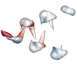
Figure 4 depicts the top and side views of the VSF isosurface of $\phi _v=0.3$ at $t=3T$. There are two sets of discrete vortex surfaces propagating towards the positive and negative $z$-directions. Each set is composed of discrete vortex surfaces generated at the end of upstroke or downstroke of the plate. From the top view in figure 4(a), a row of circular wake structures are compressed in the spanwise direction induced by TIVs. From the side view in figure 4(b), almost all the spoon-like vortex surfaces consist of TIV lines, except ring-like $V_1$ dominated by trailing-edge vortex lines.

Figure 4. The VSF isosurface of $\phi _v=0.3$ at $t=3T$ in (a) top view and (b) side view, where $D_1$ (black solid line) and $D_2$ (blue dashed line) are two types of integral domains enclosing the plate for calculating the total force in (4.3). (c) Contour of the spanwise vorticity on the spanwise symmetry plane at $y=0$.

We extract and label the discrete vortex surfaces by an automatic searching and flooding algorithm, and then track their evolution in the wake. At a particular time $t$, we count the total number, $N(t)$, of discrete vortex surfaces, e.g. $N(t=3T)=7$ in figure 4(b). For the $N(t)$ vortex surfaces, the $i$th one is labelled as $V_i$ in an ascending sequence according to its shedding time, i.e. $i=1$ is for the first shedding surface, and $i=N(t)$ is for the surface enclosing the plate.

The evolution of spoon-like vortex surfaces in the wake in figure 4(b) can be roughly split into two phases. First, the vortex surface evolves with the local induction of adjacent vortex surfaces. The upstream part of a vortex surface (e.g. $V_4$) is lifted to form a ‘nose’ by the induction of TIVs of its upstream spoon-like vortex surface (e.g. $V_5$), similar to the vortex contrail structure observed in Dong et al. (Reference Dong, Mittal and Najjar2006). In the second phase, the vortex surface evolves almost independently owing to the diminishing induction effect among separating vortex surfaces. As the spoon-like vortex surface convects downstream, its upstream nose-like structure and downstream handle-like structure are gradually smoothed out, evolving into a ring-like vortex surface (e.g. $V_2$).

The discrete vortex surface in the wake was simplified as a vortex ring for further theoretical analysis, which is detailed in Appendix B. As sketched in figure 4(c), the radius $a$ and the inclination angle $\beta$ of the vortex ring are determined by the spanwise vorticity $\omega _y$ on the spanwise symmetry plane.

4.1. Impulse theory for a finite domain

From the wake information of a flapping plate, we estimate aerodynamic forces acting on the plate using the impulse theory (see Wu Reference Wu1981; Wu et al. Reference Wu, Ma and Zhou2015). In a three-dimensional incompressible viscous flow, the total force on a moving body is

(4.1)\begin{equation} \boldsymbol{F}={-}\frac{\mathrm{d} \boldsymbol{I}_{f \infty}}{\mathrm{d} t}+\frac{1}{2} \frac{\mathrm{d}}{\mathrm{d} t} \int_{\partial B} \boldsymbol{x} \times(\boldsymbol{n} \times \rho \boldsymbol{u}) \,\mathrm{d} S, \end{equation}

where

(4.2)\begin{equation} \boldsymbol{I}_{f \infty} = \tfrac{1}{2} \int_{\mathcal{V}_{f \infty}} \boldsymbol{x} \times \rho \boldsymbol{\omega} \,\mathrm{d} V \end{equation}

is the vortical impulse in the entire fluid domain $\mathcal {V}_{f \infty }$, $\partial B$ is the body surface and $\boldsymbol {n}$ is the unit surface normal.

From the impulse theory for a finite domain $\mathcal {V}_{f}$ bounded by surface $\varSigma$ in flows with discrete wake vortices (see Wu et al. Reference Wu, Lu and Zhuang2007; Kang et al. Reference Kang, Liu, Su and Wu2018), the total force on the plate becomes

(4.3)\begin{equation} \boldsymbol{F}={-}\frac{\mathrm{d} \boldsymbol{I}_{f}}{\mathrm{d} t}- \boldsymbol{L}+\boldsymbol{F}_{\partial B}+\boldsymbol{F}_{\omega_n}+\boldsymbol{F}_{\varSigma}. \end{equation}

Here,

(4.4)\begin{equation} \boldsymbol{I}_{f} = \tfrac{1}{2} \int_{\mathcal{V}_{f}} \boldsymbol{x} \times \rho \boldsymbol{\omega} \,\mathrm{d} V, \end{equation}

denotes the vortical impulse in the finite domain $\mathcal {V}_{f}$,

(4.5)\begin{equation} \boldsymbol{L}=\int_{\mathcal{V}_{f}} \rho \boldsymbol{\omega} \times \boldsymbol{u} \,\mathrm{d} V, \end{equation}

denotes the integral of the Lamb vector $\boldsymbol {\omega } \times \boldsymbol {u}$,

(4.6)\begin{equation} \boldsymbol{F}_{\partial B} = \tfrac{1}{2} \int_{\partial B} \boldsymbol{x} \times(\boldsymbol{n} \times \rho \boldsymbol{a}) \,\mathrm{d} S+\tfrac{1}{2} \int_{\partial B} \boldsymbol{x} \times \rho \boldsymbol{u} \omega_{n} \,\mathrm{d} S, \end{equation}

denotes the force contributed by the body motion and deformation with the acceleration $\boldsymbol {a}$ of the body and the vorticity component $\omega _{n}$ normal to $\partial B$,

(4.7)\begin{equation} \boldsymbol{F}_{\omega_n}=\tfrac{1}{2} \int_{\varSigma} \boldsymbol{x} \times \rho \boldsymbol{u} \omega_{n} \,\mathrm{d} S, \end{equation}

denotes the force due to the normal vorticity on $\varSigma$ with the vorticity component $\omega _n$ normal to $\varSigma$ and

(4.8)\begin{equation} \boldsymbol{F}_{\varSigma} = \tfrac{1}{2} \int_{\varSigma}(\boldsymbol{x} \times \rho \boldsymbol{\sigma}+\boldsymbol{\tau}) \,\mathrm{d} S \end{equation}

is the viscous force calculated on $\varSigma$ with the diffusive vorticity flux $\boldsymbol {\sigma }=\nu \partial \boldsymbol {\omega } / \partial n$ and the shear stress $\boldsymbol {\tau }=\mu \boldsymbol {\omega } \times \boldsymbol {n}$. We validate that the relative discrepancy between the total forces calculated from (4.3) in the impulse theory and directly from the DNS data for the present cases is only approximately $1\,\%$.

Some terms in (4.3) can be neglected in the present cases. The thin plate with negligible deformation implies $\boldsymbol {F}_{\partial B} = 0$ owing to the vanishing $\omega _{n}$ on the body surface and opposite $\boldsymbol {n}$ on the top and bottom plates. For high $Re$, $\boldsymbol {F}_{\varSigma }$ for the viscous effect is neglected. In the present simulation with $Re=200$, the contribution of $\boldsymbol {F}_{\varSigma }$ on the total force is only approximately $0.1\,\%$. Thus, the total force of the flapping plate is determined by the vortical impulse, the Lamb-vector integral and the surface integral $\boldsymbol {F}_{\omega _n}$ over the boundary of a finite fluid domain in (4.3).

4.2. Impulse theory based on vortex surfaces

In order to further simplify (4.3), it is crucial to choose an appropriate domain boundary $\varSigma$ to minimize $\boldsymbol F_\omega$ in (4.7).

First, Kang et al. (Reference Kang, Liu, Su and Wu2018) proposed a strict constraint, $\boldsymbol {\omega }=0$ at and near $\varSigma$, to eliminate $\boldsymbol {F}_{\omega _n}$ in the minimum-domain impulse theory, but this condition is hard to satisfy in three-dimensional flows. Second, a simple domain facilitates the calculation of the surface integral in $\boldsymbol {F}_{\omega _n}$, e.g. a rectangular domain $\mathcal {V}_{f}$ enclosing the body (Wang et al. Reference Wang, Zhang, He and Liu2013). However, $\boldsymbol {F}_{\omega _n}$ is non-vanishing in (4.3), e.g. the positive contribution of $\boldsymbol {F}_{\omega _n}$ to the time-averaged thrust can be approximately $50\,\%$ in our Case 1 with $\mathcal {V}_{f} = D_1$ enclosed by the black solid line in figure 4(b). Third, an integral domain cutting a small portion of vorticity is another option to minimize $\boldsymbol F_\omega$. Li & Lu (Reference Li and Lu2012) chose a domain enclosing two discrete vortical structures near the plate, e.g. $\mathcal {V}_{f} = D_2$ enclosed by the blue dashed curve in figure 4(b), but $D_2$ should move with the vortical structure at different times and its geometry varies with different flow parameters, so it has to be determined ad hoc for different cases.

Compared with the existing options for $\varSigma$, the VSF isosurface is a more natural choice, because it has $\boldsymbol {F}_{\omega _n}=0$ with $\omega _n=0$ on $\varSigma$ and evolves with time. Based on the VSF, we choose $\varSigma$ as a particular vortex surface $\varSigma _{b}$ enclosing the plate in figure 5. In this way, (4.3) is simplified to

(4.9)\begin{equation} \boldsymbol{F}={-}\frac{\mathrm{d} \boldsymbol{I}_{b}}{\mathrm{d} t}-\boldsymbol{L}_b, \end{equation}

where

(4.10)\begin{equation} \boldsymbol{I}_{b} = \tfrac{1}{2} \int_{\mathcal{V}_{b}} \boldsymbol{x} \times \rho \boldsymbol{\omega} \,\mathrm{d} V \end{equation}

denotes the vortical impulse in a finite fluid domain $\mathcal {V}_{b}$ enclosed by $\varSigma _{b}$, and

(4.11)\begin{equation} \boldsymbol{L}_b=\int_{\mathcal{V}_{b}} \rho \boldsymbol{\omega} \times \boldsymbol{u} \,\mathrm{d} V \end{equation}

denotes the Lamb-vector integral over $\mathcal {V}_{b}$. As sketched in figure 5, $\boldsymbol F$ is only determined by the velocity–vorticity field within $\mathcal {V}_{b}$. Then we obtain the thrust force

(4.12)\begin{equation} F_T=\frac{\mathrm{d} I_{b,x}}{\mathrm{d} t}+ L_{b,x}, \end{equation}

where $I_{b,x}$ and $L_{b,x}$ are the streamwise components of $\boldsymbol {I}_{b}$ and $\boldsymbol {L}_b$, respectively.

Figure 5. Sketch of vortex surfaces in the near wake and far wake of a flapping plate.

In the present cases, the time-averaged thrust can be determined by

(4.13)\begin{equation} \bar{F}_T =\overline{\frac{\mathrm{d} I_{b,x}}{\mathrm{d} t}}+\bar{L}_{b,x} \end{equation}

over a half-period $T_f=T/2$ within either one downstroke or upstroke owing to the periodic flapping motion of the plate, where $\bar {f}$ denotes the time average of a function $f$ over $T_f$. Without loss of generality, we choose one downstroke period to estimate $\bar {F}_T$. Figure 6 sketches the formation and shedding of the $i$th vortex surface $V_i$ from the plate with $i \geq 3$. We define the beginning time $t_i'=T/4+(i-2)T_f$ of downstroke in figure 6(a), the end time $t_i''=T/4+(i-1)T_f$ of downstroke in figure 6(b) and the shedding time $t_i^s \approx t_i''+T_f = T/4+i T_f$ of $V_i$ in figure 6(c) when $V_i$ is just shed from the plate.

Figure 6. Sketch of formation and shedding of vortex surface $V_i$ at different times: (a) $t=t_i'$, the beginning time of downstroke; (b) $t=t_i''$, the end time of downstroke; (c) $t=t_i^s$, the shedding time of $V_i$. The vortex surfaces with counterclockwise and clockwise vortex lines are coloured in blue and yellow, respectively. The Lagrangian-like evolution of $\varSigma _b$ labelled at $t = t_i'$ is marked by the red dashed curves.

During the downstroke from $t=t_i'$ to $t=t_i''$ for the generation of $V_i$, the Lagrangian-like evolution of $\varSigma _b$ is marked by the red dashed curves in figure 6(a,b). Since the shedding of spoon-like vortex surfaces from the flapping plate is periodic, we estimate

(4.14)\begin{equation} \overline{\frac{\mathrm{d} I_{b,x}}{\mathrm{d} t}} = \frac{I_{b,x}(t_i'') - I_{b,x}(t_i')}{T_f} \approx \frac{I_{i-1,x}(t_{i}'')}{T_f}\approx \frac{I_{i,x}^s}{T_f} \end{equation}

in (4.13), where $I_{i,x}^s$ denotes the streamwise component of the vortical impulse

(4.15)\begin{equation} \boldsymbol{I}_{i}^s = \tfrac{1}{2} \int_{V_{i}} \boldsymbol{x} \times \rho \boldsymbol{\omega} \,\mathrm{d} V \end{equation}

for $V_i$ at its shedding time $t=t_i^s$, and all the $I_{i,x}^s = I_x^s$ are the same for $3 \le i \le N$. Then, the time-averaged thrust

(4.16)\begin{equation} \bar{F}_T =\frac{I_x^s}{T_f}+\bar{L}_{b,x} \end{equation}

acting on the plate can be estimated based on the velocity–vorticity field within $\mathcal {V}_{b}$ enclosed by the vortex surface.

For the further application, we can also estimate the force only from the shedding vortex surfaces in the near wake and far wake in §§ 4.3 and 4.4, respectively. As sketched in figure 5, the near-wake region has the discrete vortex surfaces close to the plate, and the far-wake region is remote from the plate.

4.3. Estimating thrust from the near wake

In order to estimate time-averaged forces on the plate from the wake, we extend $\bar {L}_{b,x}$ in (4.16) based on the vortex surface enclosing the plate to an expression based on discrete vortex surfaces in the wake. Since the Lamb-vector integral

(4.17)\begin{equation} \int_{\mathcal{V}_{f\infty}} \rho \boldsymbol{\omega} \times \boldsymbol{u} \,\mathrm{d} V=\boldsymbol{L}_b+\boldsymbol{L}_{wake} =0 \end{equation}

vanishes in $\mathcal {V}_{f\infty }$ (Wu et al. Reference Wu, Ma and Zhou2015), which is also validated by our DNS, we obtain

(4.18)\begin{equation} \boldsymbol{L}_b={-}\boldsymbol{L}_{wake}. \end{equation}

Considering the downstroke for generating $V_i$ from $t=t_i'$ to $t=t_i''$ in figures 6(a) and 6(b), we approximate

(4.19)\begin{equation} \boldsymbol{L}_{wake}=\sum_{j=1}^{i-2}\boldsymbol{L}_j \end{equation}

as the sum of the Lamb-vector integral

(4.20)\begin{equation} \boldsymbol{L}_j=\int_{V_j} \rho \boldsymbol{\omega} \times \boldsymbol{u} \,\mathrm{d} V, \end{equation}

for the $j$th discrete vortex surface $V_{j}$ in the wake.

Since the spoon-like vortex surface with finite $\boldsymbol {L}_j$ evolves towards a ring-like one with $\boldsymbol {L}_j\approx 0$ in the far wake, $\boldsymbol {L}_j$ decays quickly in the downstream. Hence, we estimate

(4.21)\begin{equation} \boldsymbol{L}_{wake} \approx \boldsymbol{L}_{i-2} \end{equation}

from the near-wake vortex surface in the downstroke, as shown in figures 6(a) and 6(b), and then have

(4.22)\begin{equation} \bar{L}_{b,x}={-}\bar{L}_{wake,x}\approx{-}\bar{L}_{i-2,x}, \end{equation}

where $\bar {L}_{wake,x}$ and $\bar {L}_{i-2,x}$ denote the time-averaged streamwise components of $\boldsymbol {L}_{wake}$ and $\boldsymbol {L}_{i-2}$, respectively.

Identified by the VSF isosurface at a given time, there are $N(t)$ vortex surfaces in an instantaneous flow field, and surface $V_{N-1}$ is shed into the wake in figure 5. Substituting (4.22) into (4.16) and taking $i=N-1$ yields

(4.23)\begin{equation} \bar{F}_T= \frac{I_x^s}{T_f}-\bar{L}_{N-3,x}. \end{equation}

Then, we approximate

(4.24)\begin{equation} \bar{L}_{N-3,x}=\frac{1}{T_f} \int_{t_{N-1}'}^{t_{N-1}''} L_{N-3,x} \,\textrm{d}t \approx \frac{L_{N-3,x}(t_{N-1}')+L_{N-3,x}(t_{N-1}'')}{2}, \end{equation}

where $L_{N-3,x}(t_{N-1}')$ and $L_{N-3,x}(t_{N-1}'')$ denote the streamwise components of the Lamb-vector integral for $V_{N-3}$ at $t=t_{N-1}'$ and $t=t_{N-1}''$, respectively. Considering the periodic shedding of vortex surfaces from the flapping plate in $T_f$ (also see figure 6), we have $L_{N-3,x}(t_{N-1}') \approx L_{N-1,x}(t_{N-1}^s)$ and $L_{N-3,x}(t_{N-1}'') \approx L_{N-2,x}(t_{N-1}^s)$. Finally, (4.23) is re-expressed by

(4.25)\begin{equation} \bar{F}_{T}= \frac{I_x^s}{T_f}-\frac{L_{N-1,x}+L_{N-2,x}}{2}, \end{equation}

where all the terms on the right-hand side are determined at $t=t_{N-1}^s$.

The thrust model (4.25) from the near wake is validated by the DNS result calculated from (2.7). From (4.25), the mean thrust coefficient $\bar {C}_T$ is estimated as

(4.26)\begin{equation} \bar{C}_T^N=\bar{C}_T^{I}+\bar{C}_T^{L}. \end{equation}

Here, the force contribution from the vortical impulse is

(4.27)\begin{equation} \bar{C}_T^{I}=\frac{I_x^s}{\frac{1}{2} \rho U^{2} R_{A}T_fc^2}, \end{equation}

and the contribution from the Lamb vector is

(4.28)\begin{equation} \bar{C}_T^{L}={-}\frac{L_{N-1,x}+L_{N-2,x}}{\rho U^{2} R_{A}c^2}. \end{equation}

Table 2 compares the mean thrust coefficients calculated from (2.8), (4.26) and (4.27) in Cases 1–4 listed in table 1 with the varying angle of attack, flapping frequency and Reynolds number. It is noted that the wake in the four cases consists of discrete vortex surfaces, and the force estimation for the wakes with complex topology, Cases 5 and 6, is discussed in Appendix C. We find that $\bar {C}_T^N$ estimated from the near-wake model agrees well with the DNS result $\bar {C}_T$ and the relative errors

(4.29)\begin{equation} \varepsilon = \frac{|\bar{C}_T^{model} - \bar{C}_T|}{\bar{C}_T} \end{equation}

are approximately $5\,\%$, where $\bar {C}_T^{model}$ denotes a model estimation of $\bar {C}_T$. Additionally, we validate that the near-wake model works well with $\varepsilon \approx 8\,\%$ for the case of a heaving and pitching plate around the leading edge with $Re=200$, $St=0.6$ and discrete wake topology in Li & Lu (Reference Li and Lu2012).

Table 2. Comparison of $\bar {C}_T$ from DNS, $\bar {C}_T^N$ from the near-wake model, $\bar {C}_T^I$ from the impulse model, $\bar {C}_T^F$ from the far-wake model and $\bar {C}_T^R$ from the vortex-ring model for estimating the thrust coefficient in the cases with different parameters in table 1.

By contrast, $\bar {C}_T^{I}$ only considering the vortical-impulse contribution is obviously overestimated. Hence, the negative $\bar {C}_T^{L}$ contributed from the Lamb vector provides a necessary correction to the impulse model, improving the prediction accuracy of $\bar {C}_T$ by approximately $12\,\%$.

In general, the VSF $\phi _v \in [0,1]$ is positively correlated with the vorticity magnitude. We choose the particular $\phi _v=0.3$ to discretize the vortex wake. The region enclosed by the isosurface of $\phi _v=0.3$ captures approximately $90\,\%$ of the vortical impulse of shedding vortex surfaces in the entire domain. Thus, we find that the calculation of $I_x^s$ in (4.26) for a single vortex surface is slightly underestimated by $2\,\%$, assuming the similar $I_x^s$ distribution of all the five vortex surfaces in the wake in figure 4.

For comparison, we also estimate $\bar {C}_T$ from the near-wake model (4.26) based on the isosurface of Eulerian vortex criteria $|\boldsymbol {\omega }|$ and $\lambda _2$, and obtain relatively large $\varepsilon = 17\,\%$ and $\varepsilon = 32\,\%$, respectively. The major reason is that the isosurface of $|\boldsymbol {\omega }|$ or $\lambda _2$ can have a notable difference from the vortex surface (Yang & Pullin Reference Yang and Pullin2011), so the contribution from the surface integral (4.7) cannot simply be neglected for these isosurfaces. We remark that the choice of the isocontour level of $|\boldsymbol {\omega }|$ or $\lambda _2$ is ad hoc for vortex identification, and we have tuned $|\boldsymbol {\omega }|$ and $\lambda _2$ to minimize their corresponding $\varepsilon$.

In addition, the vortex-ring model (see Lauder & Drucker Reference Lauder and Drucker2002; Nauen & Lauder Reference Nauen and Lauder2002; Li & Lu Reference Li and Lu2012) can estimate the mean thrust using the vortical impulse $I_v=\rho {\rm \pi}\varGamma a^2$ of a vortex ring, where $\varGamma$ is the circulation of the vortex ring. In Appendix B, we simplify the spoon-like vortex surface in figure 4 to the vortex ring, and determine the mean thrust coefficient $\bar {C}_T^R$ from the modelled vortex ring. In table 2, $\bar {C}_T^R$ is overestimated and has larger discrepancies than other models for our cases, perhaps owing to the over-simplification of the spoon-like vortex surfaces in figures 3 and 4 as vortex rings. We find that the time-averaged streamwise vortical impulse of ring-like $V_1$ dominated by circular trailing-edge vortex lines is approximately 40 %–50 % larger than that of the spoon-like vortex surfaces with kinked tip vortex lines.

4.4. Estimating thrust from the far wake

From the practical viewpoint, estimating forces on the moving body from the far wake is very useful in the experimental investigation of biological locomotion (Lauder & Drucker Reference Lauder and Drucker2002; Spedding et al. Reference Spedding, Rosén and Hedenström2003) and underwater vehicles (Jiménez et al. Reference Jiménez, Hultmark and Smits2010). As indicated in figure 4, a pair of discrete vortex surfaces are shed form the plate within $T$, and the wake is dominated by two rows of discrete vortex surfaces. The evolution of vortex pairs in the wake is similar owing to their periodic formation and shedding process. Thus, it is possible to estimate forces based on two arbitrary vortex surfaces in the far wake.

We define the geometrical centre of vortex surface $V_i$ as

(4.30)\begin{equation} \boldsymbol{x}_{c,i}=\frac{\displaystyle\int_{V_i} \boldsymbol{x} \,\mathrm{d}V}{\displaystyle\int_{V_i} \mathrm{d}V}. \end{equation}

Figure 7(a) shows that the vortex centre moves downstream with a uniform velocity, and the streamwise vortical impulse also linearly decays for all the discrete vortex surfaces. These linear relations are utilized to infer $I_x^s$ from the far wake.

Figure 7. Temporal evolution of (a) streamwise vortex centre $x_c$ and (b) streamwise impulse $I_x$ of discrete vortex surfaces in the wake.

We approximate the shedding location $x_{c,s} = 1.5$ for all the discrete vortex surfaces, corresponding to the position where $I_x^s$ is obtained. Given two arbitrary vortex surfaces $V_a$ and $V_b$ with $a,b = 3,\ldots ,N-1$ in the wake, we estimate the initial streamwise vortical impulse $I_x^s$ as

(4.31)\begin{equation} I_x^s\approx I_x^F = I_{a,x}+\frac{I_{a,x}-I_{b,x}}{x_{c,b}-x_{c,a}}(x_{c,a}-x_{c,s}), \end{equation}

where $x_{c,a}$ and $x_{c,b}$ respectively denote streamwise vortex centres of $V_a$ and $V_b$, and $I_{a,x}$ and $I_{b,x}$ respectively denote streamwise vortical impulses of $V_a$ and $V_b$. Then, we estimate the mean thrust coefficient

(4.32)\begin{equation} \bar{C}_T^{F}=\frac{A_L I_x^F}{\frac{1}{2} \rho U^{2} R_{A}T_fc^2} \end{equation}

from the far wake with small $a$ and $b$, where $A_L=0.85$ is an attenuation factor for the Lamb-vector correction. In this far-wake model, we estimate the thrust contributed from the vortical impulse without explicitly considering the Lamb-vector integral, because it is difficult to predict $\boldsymbol L$ at the shedding time from the far wake owing to the fast decay of $\boldsymbol L$ downstream. In order to incorporate the negative contribution of $\boldsymbol L$ to $\bar {C}_T$, we alternatively apply the factor $A_L=0.85$ in (4.32), which is estimated based on the overall ratio of $\bar {C}_T^N$ from the near-wake model and $\bar {C}_T^I$ from the impulse model listed in table 2.

The far-wake model predictions from (4.32) with $a=4$ and $b=3$ generally agree with the DNS results in table 2, and the relative errors $\varepsilon \approx 9\,\%$ are, reasonably, larger than those in the near-wake model. The thrust predictions with different $a$ and $b$ are very similar within ${\pm }3\,\%$ variation. Furthermore, we can also calculate $I_x^F$ and then estimate $\bar {C}_T^{F}$ from the Lagrangian history of a single vortex surface at different locations at two times within a small time interval.

The far-wake model (4.32) implies that the thrust of the flapping plate is determined by the vortical impulse generated during the flapping motion, and the shedding vortex surface with larger $I_x^F$ can generate larger thrust on the moving body (Spedding et al. Reference Spedding, Rosén and Hedenström2003; Li & Lu Reference Li and Lu2012), which can guide the optimization of the kinematics parameters of the flapping plate in (2.1) and (2.2) to increase the thrust of the flapping plate by shedding the vortex surface with larger $I_x^F$.

Thus, we provide a possible approach to estimate thrust using only two vortex surfaces in the wake, which can facilitate the estimation of the state of the moving body in experimental investigation and practical applications. In the experimental implementation, the particle image velocimetry (PIV) can be used to measure the three-dimensional flow field in the wake (Buchholz & Smits Reference Buchholz and Smits2008; Mendelson & Techet Reference Mendelson and Techet2015). The PIV data are usually subject to noise, so the time series of raw PIV data need to be corrected, e.g. using the divergence-free smoothing method (Wang et al. Reference Wang, Gao, Wang, Wei, Li and Wang2016). Subsequently, the boundary-constraint method (Xiong & Yang Reference Xiong and Yang2017) can be applied to construct VSFs, then the thrust is estimated based on vortex surfaces in the wake. On the other hand, significant challenges still exist in the implementation, e.g. the incompleteness of velocity/vorticity measurement, accuracy of VSF calculation from under-revolved experimental data and the uncertainty quantification of the force estimation.