


1. Introduction
The interaction of a gas with a solid surface is the foundation of many physical problems, such as boundary conditions of fluid flow on a wall, heterogeneous condensation and crystal growth. In the field of fluid mechanics, Prandtl (Reference Prandtl1904) proposed the famous boundary layer theory in 1904, which described the interaction between a traditional continuum fluid and a solid wall. But for rarefied gas flow or microscale flow, the non-equilibrium effect of the wall, known as the Knudsen layer which is located between the boundary layer and the wall, becomes very important (Gu & Emerson Reference Gu and Emerson2009; Zhang, Meng & Wei Reference Zhang, Meng and Wei2012). It is urgent to study gas–solid interactions more elaborately.
It is convenient and essential to study gas–solid interactions at the molecular level. The relationship between incidence state and reflection state of gas molecules on a solid surface can be described by a scattering kernel, which is the probability that an incident molecule with velocity  $\boldsymbol {u}_i$ is reflected with velocity
  $\boldsymbol {u}_r$. About 140 years ago, Maxwell (Reference Maxwell1878) provided the earliest scattering kernels. Two basic modes of molecular scattering which are well known today, specular reflection and diffuse reflection, were proposed. For a large number of molecules scattering from a solid surface, it is assumed that part of them comes from complete diffuse reflection and the remaining portion comes from specular reflection. The proportion of diffuse reflection is assumed to be the tangential momentum accommodation coefficient (TMAC)
  $\sigma _t$, which is constant and depends on the species of gas and the solid wall (Maxwell Reference Maxwell1879).
However, experimental studies (Maurer et al. Reference Maurer, Tabeling, Joseph and Willaime2003; Shen Reference Shen2006; Ewart et al. Reference Ewart, Perrier, Graur and Meolans2007) have shown that specular reflection and diffuse reflection models are not accurate enough to describe the scattering of gas ( $\mathrm {N_2}$ or He) molecules with the surface (Si). Epstein (Reference Epstein1967) proposed that the diffuse reflection probability
  $P(\bar {c}')$ is related to the incidence velocity
  $\bar {c}'$ and suggested a general expression for a scattering kernel with three free constants which can only be determined for specific problems. In 1971, Cercignani & Lampis (Reference Cercignani and Lampis1971) constructed another scattering kernel model that meets the normalization condition and reciprocity principle. They established scattering kernels for each component of gas molecular reflection velocity, and each scattering kernel contains a to-be-determined constant. If the surface is considered to be isotropic, then one tangential scattering kernel can be reduced. The remaining two constants are the accommodation coefficient (AC) of the normal energy
  $\alpha _{n}$ and that of the tangential momentum
  $\sigma _{t}$. Nearly two decades later, Lord (Reference Lord1995) developed the kernel and applied it to the direct simulation Monte Carlo algorithm. Then, the well-known gas–solid interaction Cercignani–Lampis–Lord (CLL) model is formed and used widely today (Bird Reference Bird1994). For example, Kalempa & Sharipov (Reference Kalempa and Sharipov2020) adopted the model to investigate the rarefied gas flow around a spherical particle and revealed the strong dependence of the thermophoretic and drag forces on the ACs.
An important issue in both Maxwell and CLL models is the difficulty of determining ACs. Generally, ACs were obtained by comparing experiment measurements with the theoretical analysis of a rarefied gas flow or microchannel flow. For example, Arkilic, Breuer & Schmidt (Reference Arkilic, Breuer and Schmidt2001) developed a precise experimental platform using a microfabrication technique to measure the mass flow rate of gas through a long microchannel. At the same time, the flow was analysed by a perturbation method based on Navier–Stokes equations with slip boundary conditions, referred to as the gas–solid interaction model. It was found that the TMAC for several gases on single-crystal silicon surface was less than unity. Veltzke & Thöming (Reference Veltzke and Thöming2012) reviewed the measurements concerning TMAC over the first decade of this century and clearly demonstrated the inconsistencies of both the measured values and the surface roughness influence on TMAC.
Moreover, the assumption that ACs are constant and independent of molecular incidence and reflection velocities may not be valid for more complex scattering situations. Benefiting from the continuous development of computer technology, direct simulation of gas–solid interactions using the molecular dynamics (MD) method (Wachman, Greber & Kass Reference Wachman, Greber and Kass1994; Yamanishi, Matsumoto & Shobatake Reference Yamanishi, Matsumoto and Shobatake1999; Barisik, Kim & Beskok Reference Barisik, Kim and Beskok2010) was used to replace the scattering kernel. Spijker et al. (Reference Spijker, Markvoort, Nedea and Hilbers2010) used the MD method to calculate the ACs and improved the velocity correlation behaviour for the existing wall models. The hybrid method (Gu, Watkins & Koplik Reference Gu, Watkins and Koplik2010; Liang, Li & Ye Reference Liang, Li and Ye2013) with direct simulation Monte Carlo, which can be used to calculate the bulk flow and MD simulating the scattering when a molecule collides with the wall surface, is popular currently. Yamamoto, Takeuchi & Hyakutake (Reference Yamamoto, Takeuchi and Hyakutake2006) used the hybrid method to calculate the flows of diatomic molecules of nitrogen in channels with a pure platinum wall and with a platinum wall with pre-adsorbed helium.
However, due to the huge computation cost of MD, direct simulation of gas–solid interactions is very expensive to apply in general physical problems. An improved or new scattering kernel which is more complex is definitely required to be constructed. Yamamoto et al. (Reference Yamamoto, Takeuchi and Hyakutake2006) considered that ACs for different variables should be determined separately. Then they proposed the Maxwell–Yamamoto model with ACs defined by normal and tangential momenta, and translation and rotation energies. Later, Yamamoto, Takeuchi & Hyakutake (Reference Yamamoto, Takeuchi and Hyakutake2007) continued to study the scattering of nitrogen with a platinum surface that adsorbs helium. They thought that part of the reflected molecules comes from the diffuse reflection model, while the other part comes from the CLL model. The ratio of the two parts and the ACs in the CLL model are all fitted parameters. However, the greatest problem with the proposed new model is that it cannot theoretically satisfy the traditional reciprocity principle. Yakunchikov, Kovalev & Utyuzhnikov (Reference Yakunchikov, Kovalev and Utyuzhnikov2012) calculated the scattering of hydrogen with a graphite surface by MD and proposed a new model, combining the Epstein model (Epstein Reference Epstein1967) with the CLL model. The parameters in the Epstein model are related to the incidence velocity of molecules, while in the CLL model the ACs are still constants. Struchtrup (Reference Struchtrup2013) promoted the Maxwell model to rough surfaces, arguing that the velocity of reflected molecules is contributed not only by specular and diffuse reflections, but also by the reflection resulting from surface roughness. The new Maxwell scattering kernel should consist of these three parts, where there are two ACs related to the velocity of incoming flow. So this model may be easier to adapt to more complex gas–solid interactions, while no systematic experimental data are available for its verification and fitting.
At the same time, compared with the establishment of new mathematical models based on traditional phenomenological models, some scholars strove to construct new gas–solid interaction models directly from the perspective of the physical collision, similar to MD simulation. The basic idea of these physical models, such as the hard cube model (Logan & Stickney Reference Logan and Stickney1966; Logan & Keck Reference Logan and Keck1968) and washboard model (Tully Reference Tully1990; Yan, Hase & Tully Reference Yan, Hase and Tully2004; Mateljevic et al. Reference Mateljevic, Kerwin, Roy, Schmidt and Tully2009), is to consider the gas–solid interaction as an elastic binary collision between gas molecules and surface cubes. However, most physical models do not meet basic boundary conditions, especially the reciprocity principle. Recently, Liang, Li & Ye (Reference Liang, Li and Ye2018) established a new gas–solid interaction model that satisfies the reciprocity principle based on the washboard model. Compared with the traditional phenomenological models, this model is more accurate and more efficient than MD simulation. However, its collision is still processed using the CLL model, and currently it cannot be applied to deterministic solvers.
Previous studies of the gas–solid interaction were always embedded in the investigation of gas flow (Peddakotla, Kammara & Kumar Reference Peddakotla, Kammara and Kumar2019), which was a natural choice since the interaction was tightly coupled to the flow. However, to reduce the computation cost of the MD method, the simulation of the gas–solid interaction is always restricted to a very small computation domain, or performed for special conditions of gas flow. Therefore, the accuracy and generalization of the scattering kernel based on the MD method need to be improved. This motivates the current study. In this paper, we decouple the gas–solid interaction from the gas flow and obtain complete data about the scattering of gas molecules on the wall surface by MD simulation. Given that MD simulations require huge computing resources, it is essential to accelerate the simulation with the parallel technology of a graphics processing unit (GPU). Then, we attempt to construct a new or improved theoretical scattering kernel by combining the simulation data with traditional phenomenological models. Based on the investigation of energy exchange during the collision, modified expressions for the kernels are provided. Compared with the probability distribution of incidence–reflection velocity determined from MD simulation, the parameters in the constructed model are determined by a machine learning program which is based on the Nesterov accelerated gradient (NAG) (Nesterov Reference Nesterov1983) algorithm and fitting evaluation criteria of minimum sum of square error and mean square error. The model for direct simulation of the gas–solid interaction and methods are described in § 2. The scattering characteristics of gas molecules on the surface and modified scattering kernels based on the CLL model are presented in § 3. In § 4, a comparison and verification of the scattering kernel models are presented. Finally, we conclude with a discussion in § 5.
2. Model and method
2.1. Model
Because the average distance between gas molecules under general conditions is much larger than the cut-off distance of intermolecular interaction, the collision of a gas molecule with a solid surface is hardly affected by other gas molecules. Assuming that the solid wall is in equilibrium, the interaction of gas flow with solid surface can be considered as many independent collisions of a gas molecule with the surface. So, the present simulation of gas–solid interaction is divided into a series of independent cases and each case includes only one gas molecule and solid surface as well, as shown in figure 1.

Figure 1. A gas molecule (blue) moves to a wall (red) from far away and interacts with the surface.
The wall consists of platinum (Pt) molecules which are arranged in a face-centred cubic crystal structure with a lattice constant of  $l_{Pt}$ and the gas–solid interface is the (1,0,0) plane. In total, 108 unit cells are established in the
  $x$,
$x$,  $y$ and
  $z$ directions (also denoted by subscripts
  $d = 1, 2, 3$ in the following) with a size of
  $6\times 6\times 3$. The length and width of the wall are several times the cut-off distance. A molecule of argon (Ar) as the gas is placed above the wall surface and the incidence height which is the same in all cases is slightly larger than the cut-off distance. Periodic conditions are applied at the wall boundaries in
  $x$ and
  $y$ directions and the incidence tangential position of the gas molecule is randomly determined. What is more important for the present model is the initial velocity of the gas molecule. Since the present work focuses on the scattering kernel which is the expression of statistical characteristic, the initial states of gas molecules in the series of simulations should keep the same statistical characteristic of the gas. In other words, each gas molecule in the simulations can be considered as a sample of all molecules in the gas flow. Assuming that the gas before the collision with the surface is in equilibrium, the initial velocity of a gas molecule is given by the random sampling method (Stickler & Schachinger Reference Stickler and Schachinger2016) based on the equilibrium Maxwellian velocity distribution (Bird Reference Bird1994):
 \begin{equation} f_e(u_{i,d})=\left\{
\begin{array}{@{}ll} \displaystyle \dfrac{1}{\sqrt{\rm \pi}}\,
\textrm{e}^{-{u_{i,d}^{2}}} , & \text{when } d=1,2\\[4pt] \displaystyle 2 u_{i,d}\,
\textrm{e}^{{-}u_{i,d}^{2}}, & \text{when } d=3,
\end{array}\right.\end{equation}
\begin{equation} f_e(u_{i,d})=\left\{
\begin{array}{@{}ll} \displaystyle \dfrac{1}{\sqrt{\rm \pi}}\,
\textrm{e}^{-{u_{i,d}^{2}}} , & \text{when } d=1,2\\[4pt] \displaystyle 2 u_{i,d}\,
\textrm{e}^{{-}u_{i,d}^{2}}, & \text{when } d=3,
\end{array}\right.\end{equation}
where the distribution function  $f$ is normalized by
  $1/ \sqrt {2R_{g}T_{g}}$ with gas constant
  $R_g$ and temperature of gas
  $T_{g}$. The subscript
  $e$ denotes the equilibrium state. Parameter
  $u_{i,d}$ is the velocity of a gas molecule normalized by
  $\sqrt {2R_{g}T_{g}}$ while the subscript
  $i$ means incidence. Only the gas molecules approaching the surface are considered in these simulations and the normal component of incidence velocity
  $u_{i,3}$ varies from zero to negative infinity. As shown in figure 2, when the number of samples, which is the number of cases to be simulated, is up to
  $100\ 000$, all the distributions of velocity components converge well to the Maxwellian distribution.

Figure 2. (a) Tangential velocity distribution of incident molecules. (b) Normal velocity distribution of incident molecules.
2.2. Method
2.2.1. The MD method
The process of scattering in every case is simulated by the MD method which can be considered essentially as an application of Newton's second law. All the interactions between molecules are described by the classical Lennard-Jones potential function:
 \begin{equation} U_{ij}=4\varepsilon\left[\left(\frac{\sigma}{r_{ij}}\right)^{12}- \left(\frac{\sigma}{r_{ij}}\right)^{6}\right],\end{equation}
where  $\varepsilon$ and
  $\sigma$ are the energy and distance parameters, respectively, their specific values being listed in table 1 (Prabha & Sathian Reference Prabha and Sathian2013). Choosing
  $m_{Pt}$,
  $\sigma _{Pt}$ and
  $\varepsilon _{Pt}$ as characteristic scales of mass, length and energy, respectively, all the variables in the following discussion have been non-dimensionalized. In addition, in order to maintain the stability of the model, the solid-wall molecules are also subjected to a spring force
  $F_{spr}=-k\Delta x$ when they deviate from their equilibrium position, which method has also been widely used (Hansen, Todd & Daivis Reference Hansen, Todd and Daivis2011). The spring coefficient
  $k=5000$ in the present work.
Table 1. Parameters of potential function.

The Velocity Verlet algorithm (Swope et al. Reference Swope, Andersen, Berens and Wilson1982) that LAMMPS (Large-scale Atomic/Molecular Massively Parallel Simulator) sets as default time advancement format is used to update the molecular positions and velocities. The time step is set as  $dt=0.001$, which is equivalent to
  $0.61635$ fs. After a sufficiently long relaxation process for wall molecules, an Ar molecule enters from the upper boundary
  $z=h=5$ to the wall surface which is at
  $z=0$. After interacting with the wall surface, the Ar molecule will be either reflected or adsorbed. If the normal distance of the Ar molecule to the wall surface exceeds
  $h$, the molecule is considered to be reflected and then the simulation is terminated. If the Ar molecule does not reflect in the whole simulation time
  $t_{Total}=3500$, which is equivalent to
  $2.16$ ns, the molecule is considered to be adsorbed by the wall.
2.2.2. The GPU acceleration algorithm
The number of cases to be simulated by MD is up to 100 000 and the total required cost of calculation is huge. Taking an Intel Core i7-8700 CPU @ 3.20 GHz as an example, the time required for a single case to run 500 time steps in a single thread is about  $25.05$ s. Roughly, it will take an average of 8 min to complete a single case, and 556 days for accomplishing all cases. This estimation indicates that a reduction of time consumption is greatly desirable.
Each case is completely independent and there is no influence on each other while the requirement of information exchange between the molecules only exists within a single case. Computational efficiency will be greatly improved by means of such parallelization of inner and outer layers. Unlike central processing units (CPUs) that focus on optimizing single-threaded execution capabilities, GPUs with a huge amount of threads provide a solution to our problem. The present work used the ‘numba’ library to implement CPU–GPU heterogeneous programming, which has become a mainstream technology for high-performance computing.
First, the outer-layer parallelism is implemented among the cases. Since the only difference between cases is the incident state of gas molecules, the outer layer can be perfectly parallelized. Then the inner-layer parallelism is effected among molecules in each single case. Due to the intermolecular interaction that needs to pass and synchronize information, this layer is less parallelized than the outer layer. Considering the CUDA execution model, each case is arranged on a thread block for calculation, and each thread in the block corresponds to a molecule. However, limited to the hardware resources of GPU, it is impossible to run all 100 000 cases at the same time. Therefore, we need to realize the function of case extraction through an algorithm. As shown in figure 3, the initial states of all cases are stored in Unfinished Cases Library (UCL). Then,  $N$ cases are extracted to
  $N$ blocks in the GPU and run at the same time. Once a case is completed, its final result is transferred to Finished Cases Library (FCL) in the CPU. A new case is immediately extracted from UCL to the thread block and the idleness of this block is greatly avoided. Of course, when the number of cases in UCL is less than
  $N$, the full load operation of thread blocks cannot be guaranteed. Finally, when all the cases are completed, the simulation terminates.

Figure 3. Schematic diagram of our CPU–GPU heterogeneous program. Here FCL and UCL represent the libraries of the finished and unfinished cases, respectively.
In order to achieve optimal operating efficiency, an independent test on a personal computer (PC) is performed to determine the appropriate number  $N$ of parallel thread blocks. The CPU used for testing is still the Inter Core i7-8700 CPU @ 3.20 GHz, while the GPU is an NVIDIA GeForce GTX 1070, which are general components for PCs. An acceleration ratio
  $\chi$ is defined to measure the operating efficiency:
 \begin{equation} \chi=\frac{Nt^{CPU}_{1}}{t^{GPU}_{N}},\end{equation}
where  $t^{CPU}_{1}$ represents the time required to run the first 500 time steps of one single case in the CPU and
  $t^{GPU}_{N}$ is the time required for the first 500 steps of parallel
  $N$ cases in the GPU. As shown in figure 4, as the number
  $N$ of parallel thread blocks increases, the acceleration ratio
  $\chi$ increases rapidly. When
  $N\ge 1000$, the improvement of operating efficiency slows down. Considering the memory requirements, we set the number of parallel thread blocks to
  $N=1000$, and the acceleration ratio is up to 320.67. This means that the amount of computation that would have taken one and a half years to complete with the CPU, can now be completed on the same PC in just a few days with GPU acceleration. Parallel technology greatly improves the computational efficiency and lays a solid foundation for future research work.

Figure 4. Relationship between acceleration ratio  $\chi$ and number of parallel thread blocks
  $N$.
$N$.
2.2.3. Machine-learning-based fitting algorithm
The present work aims to construct a scattering kernel from the direct simulation data. In traditional kernels, such as the Maxwell model and CLL model, it is always assumed that the probabilities of reflection velocity components in different directions are independent of each other. In the present work, the scattering kernel is also established for each component of reflection velocity and the kernels are denoted by  $R_d=R(u_{r, d } \mid \boldsymbol {u}_i)$ with
  $d=1, 2$ or
  $3$, where the subscript
  $r$ means reflection. Therefore, with the specified distribution of incidence velocity
  $f(\boldsymbol {u}_i)$, the probability density of molecules with reflection velocity component
  $u_{r, d }$ and incidence velocity
  $\boldsymbol {u}_i$ can be written as
 \begin{equation} p_d = R(u_{r, d} \mid \boldsymbol{u}_i)f(\boldsymbol{u}_i).\end{equation}
Inspired by previously reported kernels, the basic form for the present scattering kernel can be presupposed and only a few parameters need to be fitted from MD simulation data. This work is suitable to be done by the fitting algorithms of machine learning (Andric, Meyer & Jenny Reference Andric, Meyer and Jenny2019).
The probability density of velocity can also be obtained from MD simulations. In fact, the probability density of any reflection variable  $\varphi$ which always depends on the incidence velocity can be determined as
 \begin{equation} P(\varphi , \boldsymbol{u}_i)=\frac{N_{\varphi, \boldsymbol{u}_i}}{N_s \triangle\varphi \triangle \boldsymbol{u}_i}, \end{equation}
where  $N_s$ is the total number of molecules scattering from the surface and
  $N_{\varphi, \boldsymbol {u}_i}$ is the number of molecules with incidence velocity in the range of
  $(\boldsymbol {u}_i-\triangle \boldsymbol {u}_i /2, \boldsymbol {u}_i + \triangle \boldsymbol {u}_i /2)$ and with
  $\varphi$ in
  $(\varphi -\triangle \varphi /2, \varphi + \triangle \varphi /2)$. There is no doubt that the probability density is affected directly by the intervals
  $\triangle \varphi$ and
  $\triangle \boldsymbol {u}_i$. If the intervals are too small, due to the limited number of molecules, it may lead to excessive statistical fluctuation; if the intervals are too large, the variation of probability density cannot be shown precisely. Since the probability density of velocity is extremely small when the velocity magnitude is large (see figure 2), the range of velocity in the present work where the probability density is determined is set to be
  $(-2,2)$ in the tangential direction,
  $(-2,0)$ for incidence and
  $(0,2)$ for reflection in the normal direction. Each range is divided into grids with number of
  $N_G = 50$ and the interval velocity remains constant for all the probability calculations.
Based on the probability density of velocity by (2.4) and (2.5), the error function for the fitting algorithm is defined as
 \begin{equation} \textrm{Error}_d = \frac{1}{N_{G}}\sum_{r}\left\{\int{[ P(u_{r,d}, \boldsymbol{u}_i)- p_d]^{2} f(\boldsymbol{u}_i) \, {\textrm{d}} \boldsymbol{u}_i}\right\}. \end{equation}
It is obvious that the smaller the error, the closer is the scattering kernel to the direct simulation. Therefore, the appropriate parameters in scattering kernels can be found by minimizing the fitting error.
In addition, it can be seen that in the three-dimensional space of incidence velocity, since the velocity distribution function is known, the numerical expectation of square error can be directly calculated; and the probability distribution of reflection velocity needs to be predicted later, so we only have to do a simple average over the grid number. In this way, the error function similar to the mean square error can reduce the influence of the number of grids. Moreover, the region with greater probability is preferentially fitted and the risk of falling into a local minimum in the fitting process is also reduced.
The probability density in (2.4) and (2.5) is defined in a four-dimensional space, which includes one reflection and three incident components of velocity. Minimizing the error function directly in high-dimensional space can capture more scattering characteristics, but it also amplifies the fluctuation in the finite molecular statistics, which may lead to certain errors in the target value of machine learning. The scattering kernel can be established for a pair of reflection and incidence velocities,  $R_{d,d'}=R(u_{r, d} \mid u_{i, d'} )$, or is projected onto a two-dimensional space:
 \begin{equation} R_{d, d'} = \int R(u_{r, d} \mid \boldsymbol{u}_i)f(u_{i,m})f(u_{i,n}) \, {\textrm{d}}u_{i, m}\, {\textrm{d}}u_{i, n},\end{equation}
where  $m$,
$m$,  $n$ denote the components of incidence velocity in the other two directions, respectively. Then, another error function is defined in the two-dimensional space, considering the cumulative square error:
 \begin{equation} \textrm{Error}_{d,d'} = \sum_{i,r} \left[ \frac{N_{d,d'}}{N_{s} \Delta u_{r, d}\Delta u_{i, d'}} - R_{d, d'}f(u_{i,d'}) \right]^{2}, \end{equation}
where  $N_{d,d'}$ is the number of molecules with reflection velocity
  $u_{r,d}$ and incidence velocity
  $u_{i,d'}$.
Fitting the algorithm can make the specified function, Error, gradually approach its extreme point by iterating. The most commonly used gradient descent method, whose advance step is completely dependent on the local gradient, has two major limitations. First, as the gradient becomes smaller, the advance slows down and the fitting efficiency is seriously reduced in the later period. More importantly, the fitting cannot break through the position where the gradient is zero. When there are multiple minimum points, the gradient descent method can only fit the specified function to its first minimum. Therefore, the NAG algorithm which assumes that the gradient of the error function should be directly related to the advance acceleration rather than the speed, is used for fitting in the present work. By accumulating historical gradients, the fitting efficiency is greatly improved. At the same time, due to the existence of inertia, the fitting can easily break through the barrier after the minimum point to reach a new minimum point, so that there is a greater probability of finding the smallest minimum point.
3. Results and discussion
3.1. Scattering of equilibrium gas by direct simulation
With the GPU parallel acceleration technology, the scattering of Ar gas with temperature  $T_g=300\ \mathrm {K}$ from the Pt metal surface under the equilibrium state of
  $T_w=300\ \mathrm {K}$ has been simulated. Before establishing the scattering kernels, the scattering characteristic which is mainly depicted by the probability density defined by (2.5) is investigated based on the direct simulation data.
3.1.1. Interaction time
During the collision of gas molecule with wall surface, the molecule velocity will change continuously due to the interaction force exerted by the wall atoms. The duration of velocity variation is defined as the interaction time and its distribution of probability density is shown in figure 5. It can be seen that the interaction time of most incident molecules is less than 50, which is equal to a dimensional time of  $30.8\ \mathrm {ps}$. In general, when the incidence velocity of gas molecules is large, the interaction time converges to a smaller value; and when the incidence velocity is smaller, the interaction time of gas molecules correspondingly increases, for which the distribution range is also wider. If the incidence kinetic energy is lower, the transition between kinetic and potential energy occurs more easily and frequently, so the interaction time is longer and more uncertain, resulting in a more sufficient exchange of momentum and energy between gas molecule and wall surface. The reflection state is greatly affected by the wall surface, similar to fully diffuse reflection. On the contrary, the reflection of a molecule with higher kinetic energy is closer to the specular one.

Figure 5. Probability distributions of interaction time with incidence velocities in different directions. (a) Tangential. (b) Normal.
Especially, there are molecules with a very long interaction time, although the probability is very small. For all the 100 000 incident Ar molecules, only two of them oscillate near the surface within the whole simulation period  $t_{Total}=3500$ and they are considered to be adsorbed by the wall surface. As listed in table 2, both of the incidence velocities are very small, which may raise the possibility of being adsorbed. For the present cases, the adsorption probability of all Ar molecules, which is only
  $0.002\,\%$, is so small that the adsorption is ignored.
Table 2. Incidence state of adsorbed Ar molecules.

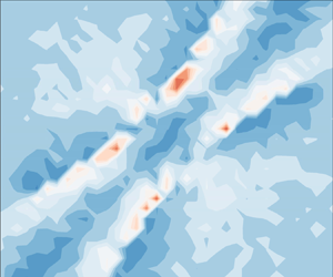
3.1.2. Distribution of reflection velocity
As the key issue of the investigation of gas–solid interactions, the probability density distribution of reflection velocity is discussed in this subsection. The classic scattering kernels are always established for a pair of velocity components in the same direction (normal or tangential to the wall) of reflection and incidence. Following the same idea, we firstly analyse the probabilities of pairs of velocity components in tangential and normal directions. As shown in figure 6, the probability distribution of tangential components presents a fusiform shape, of which two tips are sharp and the middle body is broad. It is consistent with the scattering results of Spijker et al. (Reference Spijker, Markvoort, Nedea and Hilbers2010) obtained by the MD method, although their simulation systems are completely different from those of the present work. In the normal direction, the probability shows a leaf-like distribution, which is consistent with the results of molecular beam experiments (Shen Reference Shen2006).

Figure 6. Probability density distributions of velocity components in pairs determined from MD simulation. (a) Tangential direction. (b) Normal direction.
In the sharp part of the tips, where the magnitude of the incidence velocity is large, the correlation between reflection and incidence is strong, i.e. the reflection velocities of most molecules are almost the same as the incidence ones in tangential direction and opposite in normal direction. When the magnitude of incidence velocity is small, the reflection velocities vary in a broad range and the molecular motions are affected greatly by the wall surface, which represents a loose correlation of reflection and incidence. This is consistent with the previous analysis of the interaction time. It is worth noting that both probability distributions of tangential and normal velocity are basically symmetric about leading diagonal, which can essentially be considered as the verification of the reciprocity principle (Cercignani Reference Cercignani1969; Kuščher Reference Kuščher1971; Wenaas Reference Wenaas1971).
3.1.3. Energy exchange
The interaction of gas molecules with the wall is always accompanied by conversions among the molecular kinetic energy, wall atomic kinetic energy and potential energy. It is obvious that the energy conversions will affect the molecule scattering characteristics.
Instead of discussing the complicated process of energy conversion, the kinetic energy change of gas molecules between after and before the collision with the wall is used to analyse the energy conversion feature. Firstly, the average total kinetic energy of the molecules with normal velocities of incidence  $u_{i,3}$ and reflection
  $u_{r,3}$,
 \begin{equation} \triangle E=\sum_{d=1}^{3}{(u_{r,d}^{2}-u_{i,d}^{2})}, \end{equation}
is determined from the MD simulation data and the distribution is shown in figure 7(a). Here, the frame of  $u_{i,3}$–
 $u_{r,3}$ is randomly chosen to illustrate the distribution and the results are similar in other frames of different velocity components. It can be seen that in most regions where there are more incidence molecules, the change of the total kinetic energy is extremely small, not exceeding
  $0.02$. For the molecules with larger velocities whose incidence probabilities are low, the average kinetic energy change with obvious statistical fluctuation is still less than
  $0.1$. Basically, under the current simulation condition, the total kinetic energy of gas molecules only changes slightly during the interaction with the wall. Because of the relatively weak interaction between Ar and Pt, the collision of gas molecules with the wall is similar to an elastic process and the molecular kinetic energy is almost conserved. If the gas–solid interaction becomes stronger, as shown in Appendix A, a large amount of energy exchange occurs between the eventually scattered molecules and the wall.

Figure 7. Kinetic energy changes of gas molecule after and before collision with the wall. (a) Total kinetic energy. (b) Kinetic energy in tangential (colours and legend) and normal (lines and labels) directions.
As mentioned in the previous subsection, the reflection velocity of molecules with a specified incidence velocity can vary in a wide range. Therefore, the reflection velocity can be totally different from the incidence velocity. Since the total kinetic energy almost keeps constant, the kinetic energy has to exchange in different directions. The change of average kinetic energy in the tangential direction,
 \begin{equation} \triangle E_t=\sum_{d=1}^{2}{(u_{r,d}^{2}-u_{i,d}^{2})}, \end{equation}
is also determined from the MD simulation data and the distribution is shown in figure 7(b) via the colours. The change of normal kinetic energy which is calculated by  $\triangle E_n=u_{r,3}^{2}-u_{i,3}^{2}$ is also shown in the figure via the lines for comparison. Of course,
  $\triangle E_n$ can be determined from the simulation data and the distribution is the same as that calculated directly but with slight statistical fluctuation. It is easy to see that, as expected, the decrease of tangential kinetic energy increases the normal kinetic energy, and vice versa. The exchange of kinetic energy between tangential and normal directions should be considered in the restructuring of scattering kernels.
3.2. Scattering kernel based on CLL model
As a classic scattering kernel which is also used widely, the CLL model is the first choice for reconstructing the scattering characteristics of gas molecules simulated by the MD method. As mentioned before, the CLL model assumes that there is no coupling between tangential and normal components of the velocity and the dimensionless form of the scattering kernel is written as
 \begin{align} R_{C,d}=\left\{
\begin{array}{@{}ll} \displaystyle
\dfrac{1}{\sqrt{{\rm \pi}\sigma_t(2-\sigma_t)}}
\exp\left\{-\dfrac{[u_{r,d}-(1-\sigma_t)u_{i,d}]^{2}}{\sigma_t(2-\sigma_t)}\right\},
& \text{when } d=1,2\\[12pt]
\displaystyle \dfrac{2 u_{r,d}}{\alpha_n}
\exp\left[-\dfrac{u_{r,d}^{2}+(1-\alpha_n)u_{i,d}^{2}}{\alpha_n}\right]
I_0\left(\dfrac{2\sqrt{1-\alpha_n} u_{r,d}
u_{i,d}}{\alpha_n}\right) , & \text{when } d=3,
\end{array}\right.\end{align}
\begin{align} R_{C,d}=\left\{
\begin{array}{@{}ll} \displaystyle
\dfrac{1}{\sqrt{{\rm \pi}\sigma_t(2-\sigma_t)}}
\exp\left\{-\dfrac{[u_{r,d}-(1-\sigma_t)u_{i,d}]^{2}}{\sigma_t(2-\sigma_t)}\right\},
& \text{when } d=1,2\\[12pt]
\displaystyle \dfrac{2 u_{r,d}}{\alpha_n}
\exp\left[-\dfrac{u_{r,d}^{2}+(1-\alpha_n)u_{i,d}^{2}}{\alpha_n}\right]
I_0\left(\dfrac{2\sqrt{1-\alpha_n} u_{r,d}
u_{i,d}}{\alpha_n}\right) , & \text{when } d=3,
\end{array}\right.\end{align}
where  $I_{0}(z)=({1}/{{\rm \pi} })\int ^{{\rm \pi} }_{0}\, \textrm {e}^{z \cos \theta }\, \mathrm {d}\theta$ is the first type of zero-order modified Bessel function. Here
  $\sigma _t$ and
  $\alpha _n$ are the ACs for tangential momentum and normal energy, respectively. Both ACs are assumed to be constant and their values should be determined by means of molecular beam experiments, or fitting the data from MD simulation with the above formulae. Unfortunately, the error calculated by (2.8) in the fitting process cannot be reduced to an acceptable level with any values in the range
  $(0,2)$ for the ACs. This indicates that the assumption of constant ACs should be given up and ACs should vary with the state, especially velocity, of the incident molecules (Yamamoto et al. Reference Yamamoto, Takeuchi and Hyakutake2007; Yakunchikov et al. Reference Yakunchikov, Kovalev and Utyuzhnikov2012).
Let the probability predicted by the CLL model equal that calculated from the direct simulation, and ACs can be solved for pairs of velocity components in different directions. Assuming that ACs only depend on the incidence velocity, the average reflection velocity  $\langle u_{r,d} \rangle =\int { u_{r,d} R_{C,d}\, \mathrm {d}u_{r,d}}$ will be the same as that predicted by the classical CLL model:
 \begin{align}
\langle{u}_{r,d}\rangle=\left\{ \begin{array}{@{}ll}
(1-\sigma_t)u_{i,d} , & \text{when } d=1,2\\[6pt] \displaystyle \dfrac{\sqrt{{\rm \pi} \alpha_n}}{2}
\exp( -\mu ) \{I_{0}( \mu ) + 2 \mu [ I_{0}( \mu ) + I_{1}(
\mu ) ] \} , & \text{when } d=3,
\end{array}\right.\end{align}
\begin{align}
\langle{u}_{r,d}\rangle=\left\{ \begin{array}{@{}ll}
(1-\sigma_t)u_{i,d} , & \text{when } d=1,2\\[6pt] \displaystyle \dfrac{\sqrt{{\rm \pi} \alpha_n}}{2}
\exp( -\mu ) \{I_{0}( \mu ) + 2 \mu [ I_{0}( \mu ) + I_{1}(
\mu ) ] \} , & \text{when } d=3,
\end{array}\right.\end{align}
where  $\mu = (({1 - \alpha _n})/{2 \alpha _n}) u_{i, d}^{2}$.
  $I_{1}(z)=({1}/{{\rm \pi} })\int ^{{\rm \pi} }_{0}\, \textrm {e}^{z \cos \theta }\cos \theta \, \mathrm {d}\theta$ is the first type of first-order modified Bessel function. So combining equations (3.4) and (4.4), ACs still can be considered as the proportion of diffuse reflection. As shown in figure 8,
  $\sigma _t$ varies in the range
  $(0,2)$ and
  $\alpha _n$ in the range
  $(0,1]$. Except for the domain around the diagonals of
  $u_{i,1}=u_{r,1}$ or
  $u_{i,3}=-u_{r,3}$, ACs are about
  $0.5$, which represents the combination of half of the specular reflection and half of the diffuse reflection. In the diagonal domain, ACs have values much less than
  $0.5$, corresponding to the specular reflection. Next to the two sides of the diagonal, there are two diffuse reflection regions where ACs are close to
  $1.0$. Moreover, the tangential momentum AC in the diffuse region with relatively small velocity exceeds
  $1.0$, which indicates the tangential velocity is also reversed.

Figure 8. Distributions of ACs: (a)  $\sigma _t$; (b)
  $\alpha _n$.
To conveniently utilize the scattering kernel, it is necessary to seek proper expressions for ACs. When ACs vary with incidence velocity, the scattering kernels of the CLL model depend on all components of incidence velocity in fact. However, pre-specifying expressions of ACs and projecting the kernels onto two-dimensional space as in (2.7), we still obtain the kernels for the velocity components in pairs with the same direction to reproduce the probability distributions as shown in figure 6. According to the analysis results of figure 7, there is a large amount of exchange between the kinetic energy of gas molecules in different directions. It can be considered that the state of molecules after reflection must be related to the incidence kinetic energy in the other two directions. By introducing the ‘kinetic energy term’  $\xi u_{i}^{2}$, we give the following AC correction expressions:
 $$\begin{gather} \sigma_t = \sigma_0 \exp[-(\xi_{1}u_{i,d'}^{2}+\xi_{3}u_{i,3}^{2})], \end{gather}$$
 $$\begin{gather}\alpha_n = \alpha_0 \exp[-(\xi_{2}u_{i,1}^{2}+\xi_{2}u_{i,2}^{2})], \end{gather}$$
where  $\sigma _0$,
  $\alpha _0$ and
  $\xi _{k} (k=1,2,3)$ are constant parameters to be determined by the fitting process. Since the wall is isotropic in the present work, the parameters in (3.5) are the same in the two tangential directions but
  $\sigma _t$ is affected indeed by the velocity component in the other tangential direction
  $u_{i,d'}$. Parameter
  $\alpha _0$ is set to be in the range
  $(0,1]$ such that
  $\alpha _n$ is also in the same range, which is consistent with the classical definition of ACs. But the upper bound of
  $\sigma _0$ is set to be in the range
  $(0,2)$ such that the special cases where the direction of tangential velocity is reversed can be included, too. It can be seen from the expression that a smaller kinetic energy will make ACs larger, resulting in a reflection mode closer to the diffuse one. When the kinetic energy of the incident molecule increases, ACs gradually decrease and eventually approach zero. The reflection is similar to the specular one.
Based on the present MD data, that is, the distribution of reflection velocity in the scattering of Ar gas in  $300\ \mathrm {K}$ equilibrium state with a
  $300\ \mathrm {K}$ Pt wall, all the parameters are determined by the fitting algorithm:
 $$\begin{gather} \sigma_0=1.194, \quad \xi_{1}=1.114, \quad \xi_{3}=0.431; \end{gather}$$
 $$\begin{gather}\alpha_0=0.964, \quad \xi_{2}=0.970. \end{gather}$$
As shown in figure 9(a), the error in the fitting process is quickly reduced to a very small level with respect to the initial value.

Figure 9. Evolution of fitting Error in two-dimensional space (a) and in four-dimensional space (b).
Then, the probability distributions of tangential and normal velocity predicted by the CLL model with varying ACs (MCLL for short in the following) are shown in figure 10, where the probabilities determined from MD simulations are also shown for comparison. It can be seen that they agree very well with each other, which indicates that the modification for ACs is acceptable. The value of  $\sigma _0$ is slightly greater than 1, which is consistent with the varying range of
  $\sigma _t$ shown in figure 8. In other words, this MCLL model can better describe the cases where the tangential velocity is reversed, although the proportion is small. In addition, the values of kinetic energy parameters
  $\xi _{k}$ are not small, so the effects of kinetic energy in the other two directions on the ACs cannot be ignored.

Figure 10. Comparison of probability distributions of velocity components in pairs obtained with the modified CLL model (lines) with those obtained with the MD simulation (colours). (a) Tangential velocity. (b) Normal velocity.
As mentioned previously, the reconstructed MCLL kernels depend on all components of incidence velocity. It is easy to obtain the probability distribution of reflection velocity over any component of incidence velocity. For example, the probability densities of  $u_{r,2}$ and
  $u_{r,3}$ over
  $u_{i,1}$ are calculated by the kernels as
 \begin{equation} p(u_{r,d},u_{i,1})=\int R_{C,d}f(u_{i,1})f(u_{i,2})f(u_{i,3})\, {\textrm{d}}u_{i,2}\, {\textrm{d}}u_{i,3},\quad d=2,3.\end{equation}
As shown in figure 11, the contour lines of  $p(u_{r,2},u_{i,1})$ appear as a series of concentric circles, which agrees well with the distribution of
  $P(u_{r,2},u_{i,1})$ determined from MD simulations. This indicates that the probability of tangential reflection velocity is hardly affected by the incidence velocity component in the other tangential direction. Perhaps this is the reason why the classic scattering kernel, which is only about a pair of velocity components in the same direction, is able to capture the primary characteristics of gas–solid interaction. It should be noted that the MCLL model is an extension of the classic kernel and therefore it keeps all the advantages of the classic kernel and has specified ACs. However, there are significant deviations between the distribution of
  $p(u_{r,3},u_{i,1})$ by MCLL and
  $P(u_{r,3},u_{i,1})$ by MD simulations, which is a defect in the new model that cannot describe the correlation between the normal reflection velocity and the tangential incidence velocity.

Figure 11. Comparison of probability distributions of reflection velocity component over incidence one in different directions obtained with MCLL model (lines) with those obtained with MD simulation (colours).
To observe more clearly the correlation between normal reflection velocity and tangential incidence velocity, the conditional probability  $P(u_{r,3} \mid u_{i,1})=P(u_{r,3},u_{i,1})/ f(u_{i,1})$ is calculated by eliminating the distribution
  $f(u_{i,1})$. It is also the probability of
  $u_{r,3}$ when the distribution of
  $u_{i,1}$ is uniform. It can be seen in figure 12 that there are two symmetric specular-like reflection regions, revealing a possible strong correlation between normal reflection velocity and tangential incidence velocity. This non-negligible correlation is analysed and considered in detail in the next section.

Figure 12. The correlation between normal reflection velocity and tangential incidence velocity.
3.3. Joint scattering kernel model
Because ACs in the MCLL model depend on incidence velocity and the scattering kernels are functions with four variables, the fitting for ACs should be carried out in a four-dimensional space. However, the fitting for ACs in the MCLL model is still based on the error in a two-dimensional space (2.8), the same as traditional kernels which are functions of only two variables, i.e. pairs of reflection and incidence velocity components. In this way, well-matched distributions in the same direction have been obtained indeed but some other key information is lost, resulting in the correlation of velocities in different directions of the kernel deviating obviously from the MD simulations. Therefore, a more accurate and reasonable scattering kernel needs to be reconstructed by a new model with better interpretability.
There is no universal expression for the scattering kernel so far. Based on probability theory (Rosen Reference Rosen2019), the joint probability in (2.4) can also be calculated as
 \begin{align} R(u_{r, d} \mid \boldsymbol{u}_i)f(\boldsymbol{u}_i)&= \sum_{d'=1}^{3}R(u_{r, d} \mid u_{i,d'})f(u_{i,d'}) \nonumber\\ &\quad - \sum_{d'=1}^{3} R(u_{r, d} \mid u_{i,d'} \cup u_{i,d'+1})f(u_{i,d'} \cup u_{i,d'+1}) \nonumber\\ &\quad + R(u_{r, d} \mid u_{i,1} \cup u_{i,2} \cup u_{i,3})f(u_{i,1} \cup u_{i,2} \cup u_{i,3}), \end{align}
where the subscript  $d' +1$ returns to
  $1$ when
  $d' = 3$. Then, dividing both sides of the above equation by
  $f(\boldsymbol {u}_i)$, it is easy to obtain an alternative method to calculate the scattering kernel. The first three terms on the right-hand side are similar to the CLL model. Unfortunately, the other terms, conditional probabilities of those duplicates, are completely unknown models and difficult to be expressed. But what we need is a potential expression for the scattering kernel, and therefore we can assume an expression as follows based on the first three terms, which may be an acceptable choice because of the small fitting error:
 \begin{equation} R(u_{r, d} \mid \boldsymbol{u}_i)=\sum_{d'=1}^{3} \zeta_{d, d'} R(u_{r, d} \mid u_{i, d'}), \end{equation}
where  $\zeta _{d, d'}$ are constants, which represent the impact ratio of each term on the scattering kernel. The terms
  $R(u_{r, d} \mid u_{i, d'})$ with
  $d=d'$ which are almost the same as CLL kernels can be determined directly. But the terms with
  $d' \neq d$ which do not appear in CLL kernels need to be customized. Inspired by the CLL model, we get a series of variants of the scattering kernel. For the tangential kernels (
 $d=1$ or
  $2$), all three terms (
 $d'=1, 2$ and
  $3$) have the same form:
 \begin{equation} R(u_{r, d} \mid u_{i, d'}) = \frac{1}{\sqrt{{\rm \pi}\sigma_{d,d'}(2 - \sigma_{d,d'})}}\exp\left\{-\frac{[u_{r, d} - (1 - \sigma_{d,d'})u_{i, d'}]^{2}}{\sigma_{d,d'}(2 - \sigma_{d,d'})}\right\}. \end{equation}
And for the normal reflection velocity ( $d=3$):
 \begin{align} & R(u_{r, 3} \mid u_{i,
d'}) \nonumber\\ &\quad = \left\{\begin{array}{@{}ll}
\displaystyle \dfrac{2u_{r,
d}}{\alpha_{d'}}\exp\left\{-\dfrac{\left[u_{r, d} - \sqrt{1
- \alpha_{d'}} \mid u_{i, d'} \mid
\right]^{2}}{\alpha_{d'}}\right\}, & \text{when } d' = 1, 2 \\[15pt] \displaystyle \dfrac{2u_{r,
d}}{\alpha_{d'}}\exp\left\{-\dfrac{u_{r, d}^{2} - (1 -
\alpha_{d'})u_{i, d'}^{2}}{\alpha_{d'}}\right\}
I_0\left(\dfrac{2\sqrt{1 - \alpha_{d'}}u_{r, d}u_{i,
d'}}{\alpha_{d'}}\right), & \text{when } d' = 3. \end{array}\right.
\end{align}
\begin{align} & R(u_{r, 3} \mid u_{i,
d'}) \nonumber\\ &\quad = \left\{\begin{array}{@{}ll}
\displaystyle \dfrac{2u_{r,
d}}{\alpha_{d'}}\exp\left\{-\dfrac{\left[u_{r, d} - \sqrt{1
- \alpha_{d'}} \mid u_{i, d'} \mid
\right]^{2}}{\alpha_{d'}}\right\}, & \text{when } d' = 1, 2 \\[15pt] \displaystyle \dfrac{2u_{r,
d}}{\alpha_{d'}}\exp\left\{-\dfrac{u_{r, d}^{2} - (1 -
\alpha_{d'})u_{i, d'}^{2}}{\alpha_{d'}}\right\}
I_0\left(\dfrac{2\sqrt{1 - \alpha_{d'}}u_{r, d}u_{i,
d'}}{\alpha_{d'}}\right), & \text{when } d' = 3. \end{array}\right.
\end{align}
Among them,  $\sigma _{d,d'}$ and
  $\alpha _{d'}$ are the corresponding ACs of tangential momentum and normal energy, respectively. Since the influences of all the incidence velocity components are included in the three terms, ACs are assumed to be constant here. Considering the difference between the incidence velocity distributions in tangential and normal directions, the expression for the normal–tangential term (
 $d=3$,
  $d'=1$ or
  $2$) comes from the hybrid of the tangential and normal CLL kernels. Moreover, since the wall surface is isotropic, it is reasonable to adopt the magnitude of tangential incidence velocity in the terms. The scattering kernel defined in (3.11) can be considered as a combination of three CLL-like kernels.
Considering the isotropy of the wall, the parameters about two tangential directions of incidence velocity are interrelated, i.e.  $\zeta _{1,1}=\zeta _{2,2}$,
  $\zeta _{1,2}=\zeta _{2,1}$, and
  $\sigma$ is similar;
  $\zeta _{3,1}=\zeta _{3,2}$,
  $\alpha _1=\alpha _2$. So, there are six parameters for the tangential kernel and four parameters for the normal one to be determined through the machine learning algorithm. As shown in figure 9(b), the error in the fitting process decreases with oscillation to an acceptable level. Under the same initial conditions as in the previous section, the final fitted parameters are listed in table 3.
Table 3. Values of parameters in the joint scattering kernel.

The error function defined as (2.6) is evolved in a four-dimensional space and the kernels are also reconstructed in this space. However, it is not convenient to observe the kernels directly in the four-dimensional space. The probability densities of reflection velocity based on the present joint kernels are then projected onto a two-dimensional space:
 \begin{align} p'_{u_{r, d}, u_{i, d'}} & = \int_{k \neq d'} R(u_{r, d} \mid \boldsymbol{u}_i) f(\boldsymbol{u}_i) \, {\textrm{d}}u_{i, k}\nonumber\\ & = f(u_{i, d'})\left[\zeta_{d, d'} R(u_{r, d} \mid u_{i, d'}) + \sum_{k \neq d'} \zeta_{d, k} H_{k}(u_{r, d})\right], \end{align}
where
 \begin{equation} H_{k}(u_{r, d}) = \int R(u_{r, d} \mid u_{i, k}) f(u_{i, k}) \, {\textrm{d}}u_{i, k}.\end{equation}
The probability distributions for pairs of reflection and incidence velocity components are shown in figure 13, where the probabilities determined from MD simulations are demonstrated again for comparison.

Figure 13. Comparison of probability distributions of reflection and incidence velocity components in pairs between the joint kernels (lines) and MD simulation (colours).
It can be seen that the present joint kernels capture correctly the probability densities of all pairs of velocity determined by MD. It should be also noted that, comparing with MD results, the error of probability density in the same direction by the joint kernel is slightly larger than that by the MCLL model. As mentioned before, the joint kernel is reconstructed in four-dimensional space, while MCLL is in two-dimensional space, with the same data from MD simulation. The total number of cases simulated in the present work is still insufficient for the fitting in four-dimensional space. Moreover, the expressions for joint kernels that we have chosen with guesses may not conform to physical reality to a certain extent. However, we have also tested other forms of scattering kernel, which are all worse than the chosen one. Although the kernel accuracy in the same direction is slightly sacrificed, the accuracy in different directions has been greatly improved, as shown in figure 13(c,d). Overall, the joint kernels are able to catch all the scattering characteristics predicted by MD simulation.
It can be seen from (3.11) and table 3 that the joint kernel for tangential reflection velocity includes three terms: CLL model in the same tangential direction with  $\sigma _t=\sigma _{d,d} = 0.201$; specular reflection in the other tangential direction where
  $\sigma _{d,d'} = 0.075$ is very close to zero; and diffuse reflection in normal direction (
 $\sigma _{d,3} = 1.002$). In addition, the proportional ratio of the second term
  $\zeta _{d,d'}=0.074$ is much less than the other two terms, which indicates the influence of the reflection in different tangential directions can be basically ignored. At the same time, since
  $\sigma _{d,3} \approx 1$, the normal incidence velocity hardly affects the third term and the term reduces to equilibrium Maxwellian distribution of
  $u_{r,d}$. To sum up, the four-dimensional joint scattering kernel in the tangential direction (
 $d=1$ or
  $2$) can be written approximately as
 \begin{equation} R(u_{r,d} \mid \boldsymbol{u}_i) \approx 0.5 R_{C,d}(u_{r, d} \mid u_{i, d}) + 0.5 f_e(u_{r, d}), \quad d=1 \text{ or } 2. \end{equation}
Therefore, the probability of tangential reflection velocity mainly depends on the incidence velocity in the same direction. The second term on the right-hand side of the above equation cannot be ignored and it further implies that the pure traditional CLL model is not accurate enough.
In addition, although the form of this two-term sum is the same as the Maxwell model, there is an essential difference between them. For a given monochromatic beam, there would be a sharp maximum in the number of molecules per unit angle at the angle corresponding to specular reflection, that is, there is a highly concentrated (infinitely narrow distribution) probability density. As Cercignani & Lampis (Reference Cercignani and Lampis1971) mentioned, this situation caused by the Dirac delta function is contradicted by experiments, so the Maxwell model is unrealistic. The AC  $\sigma _t$ in the first term cannot be approximated to zero, so the sharp maximum can be avoided. This shows that the physical real scattering is far beyond the description of specular reflection.
As for the joint kernel of normal reflection velocity, it is affected not only by the normal incidence velocity which is described by the normal CLL model with  $\alpha _n = \alpha _{3} = 0.075$ but also by the tangential velocity described by the hybrid CLL model with
  $\alpha _{1} = \alpha _{2} = 0.203$. Considering the same influence of two tangential incidence velocities and proportional ratio in table 3, the normal joint kernel can be written as an approximate formula:
 \begin{equation} R(u_{r, 3} \mid \boldsymbol{u}_i) \approx 0.5 R_{C,3}(u_{r, 3} \mid u_{i, 3}) + 0.2 R(u_{r, 3} \mid u_{i, 1}). \end{equation}
The second term shows clearly the correlation of tangential incidence velocity to the normal kernel, which has been revealed by MD simulations and cannot be described by the previous two-dimensional scattering kernels. The AC of tangential kinetic energy can be calculated using the formula  $\alpha _{t} = \sigma _{1, 1} (2 - \sigma _{1, 1}) = 0.362$. From the definition of
  $\alpha$, when the wall temperature does not change, the magnitude of
  $\alpha$ is proportional to the amount of energy exchanged before and after the molecule collides with the wall. Since
  $\alpha _t > \alpha _n = \alpha _3 = 0.075$, it shows that the rate of change of normal energy before and after the collision is smaller than that of tangential energy. The collision is dominated by the normal motion, and the kinetic energy tends to be conserved; while the unevenness of the wall composed of molecules means that the tangential motion of the molecules easily produces large changes, so the rate of change of kinetic energy is greater.
In general, the configuration of the joint kernel agrees better, on the whole, with that of the MD result.
4. Discussion
The aim of establishing the scattering kernel is to predict the velocity distribution of very large numbers of molecules reflected from a wall:
 \begin{equation} f(u_{r, d})=\int R(u_{r, d} \mid \boldsymbol{u}_i) f(\boldsymbol{u}_i) \, {\textrm{d}} \boldsymbol{u}_i. \end{equation}
If the molecules are in equilibrium before the reflection, i.e. the incidence velocity satisfies the Maxwellian velocity distribution (2.1), it is well known that the reflection velocity distribution predicted by the traditional CLL model, as well as the present joint kernels which essentially belong to the CLL model, satisfies the Maxwellian distribution, too. Due to the varying of ACs with the incidence velocity in MCLL kernels, the reflection velocity distribution predicted by MCLL kernels can be obtained by numerical integration. As shown in figure 14, the reflection velocities in both tangential and normal directions also converge to the Maxwellian velocity distribution, and agree very well with the distributions obtained by MD simulations which are also shown for comparison. This verifies the reliability of the present reconstructed kernels.

Figure 14. Distributions of reflection velocity obtained with the modified CLL model and MD simulations.
If the incidence velocity distribution is not in equilibrium, but is specified, such as that in molecular beam experiments, the average variables of reflection can be calculated via the scattering kernels. Then, the average ACs of energy  $E$ and momentum
  $\tau$ which are applied very widely to depict the energy and momentum exchange between gas flow and solid wall are defined as
 $$\begin{gather} \textrm{EAC} = \frac{\langle E_i\rangle - \langle E_r\rangle }{\langle E_i\rangle - \langle E_w \rangle}, \end{gather}$$
 $$\begin{gather}\textrm{TMAC} = \frac{\langle \tau_i\rangle - \langle \tau_r\rangle }{\langle \tau_i\rangle -\langle \tau_w\rangle}, \end{gather}$$
where the subscript  $w$ denotes the equilibrium state of the reflected gas molecules with the solid wall. We carried out the numerical experiments of a molecular beam discussed by Liang et al. (Reference Liang, Li and Ye2018) based on MD simulation and the washboard model, to examine the present reconstructed scattering kernels. The experiments include two groups where the effects of incidence velocity magnitude and direction on the average ACs are investigated. In the first group, the incident direction remains unchanged and the kinetic energy normalized by
  $k T_g$,
  $E=\sum _{d=1}^{3} u_{i,d}^{2}$, varies in the range
  $(0.54, 5.0)$. In the second group, the incident direction inclines from the perpendicular to the wall surface, i.e. the incident angle
  $\theta$ increases from
  $0$ to about
  $70^{\circ }$, with constant kinetic energy. In order to inspect the normal and tangential kernels respectively, EAC is calculated here by the normal kinetic energy
  $u_3^{2}$ and TMAC by tangential velocity
  $u_1$.
Based on the equilibrium distribution, it is found that  $\langle u_{w,3}^{2} \rangle =1$. From the definition of EAC, there may exist a singularity when
  $\langle u_{i,3}^{2}\rangle =1$. For a CLL-like kernel, if ACs do not depend on the reflection velocity, the average normal reflection kinetic energy can be described as
 \begin{equation} \langle u_{r,3}^{2}\rangle = (1-\alpha_n) u_{i,3}^{2}+\alpha_n.\end{equation}
So, for the MCLL kernel with variable ACs,  $\textrm {EAC}\approx \alpha _n$ and the singularity vanishes. But for the joint kernel (3.17), the second term which describes the correlation between the normal reflection velocity and tangential incidence velocity will bring additional contribution to
  $\langle u_{r,3}^{2}\rangle$. Then, the singularity still exists in the joint kernel. The EAC calculated by MCLL and joint kernel in the two experiments are shown in figure 15, where EAC determined from MD simulations and provided by Liang et al. (Reference Liang, Li and Ye2018) are also shown for comparison. It can be seen that although there are differences between Liang's result and the present MD simulation, the variation trends of EAC agree with each other. The EAC predicted by the joint kernel agrees exactly with that by MD simulation in both experiments, including the existence of the singularity. At the same time, EAC given by MCLL follows
  $\alpha _n=\alpha _0 \exp {(-\xi _2 E\sin ^{2}\theta )}$, as analysed above, which deviates from the MD results obviously. Therefore, for the reflection normal velocity, the joint kernel describes the scattering characteristics better.

Figure 15. Variation of the average ACs with incidence kinetic energy (a) and incidence angle (b) in molecular beam experiments.
Considering that the average tangential velocity in equilibrium state with the solid wall is zero and the incidence velocity is specified in the experiments, TMAC can be derived via the average reflection tangential velocity which can be calculated by the kernels. For the joint kernel, by the approximate form in (3.16),  $\langle u_{r,1}\rangle \approx 0.5(1-\sigma _{1,1})u_{i,1}$, where the second term in the kernel does not contribute to the average reflection velocity. Then,
  $\textrm {TMAC}\approx 0.5(1+\sigma _{1,1})$ is almost constant, as shown in figure 15. As for the MCLL model,
  $\langle u_{r,1}\rangle$ is described in (3.4), so
  $\textrm {TMAC}=\sigma _t$, which depends on the incidence kinetic energy. As shown in figure 15, when the incidence kinetic energy increases,
  $\sigma _t$ as well as TMAC decreases; with unchanged incidence kinetic energy, the incidence angle hardly affects
  $\sigma _t$ and TMAC. Due to the limited number of MD cases whose initial state satisfies the conditions of the two experiments, the statistical fluctuation of TMAC by MD is obvious but it still can be seen that TMAC decreases slightly with increasing incidence kinetic energy, especially when the energy is not very large. This variation trend is captured correctly by the MCLL model, which is better than that of the joint kernel for the tangential reflection velocity.
5. Conclusion
In the present work, scattering of gas molecules from a solid wall surface was simulated by the MD method and more accurate data-based scattering kernels were reconstructed from the direct simulation data.
With GPU parallel technology, the MD simulation of molecule scattering was excellently accelerated. The scatterings of gas molecules were divided into many independent cases and the simulation of each case was assigned to a thread block where the movement of each molecule was calculated by a thread. The complete independence between the cases and interaction between molecules in single case resulted in a typical external–internal double-layer parallel structure. This structure ultimately enabled the present CPU–GPU heterogeneous program to achieve an acceleration ratio of up to 320, greatly improving the efficiency of studying scattering kernels.
The present MD simulations perfectly reproduced the fusiform and leaf-shaped velocity distribution contour structures in molecular beam experiments (Shen Reference Shen2006), which could not be predicted well by the existing theoretical models. Then, the NAG algorithm and error criteria were used to reconstruct scattering kernels from MD simulation data. Based on the CLL model which is used widely, two modified scattering kernels were proposed. The first one is named as MCLL and adopts variable ACs and the second one is a joint model of three CLL-like kernels. The ACs in the MCLL model are expressed by the functions of incidence velocity with parameters fitted in a two-dimensional space such that the MCLL model can accurately predict the probability distributions of velocity pairs of reflection and incidence in the same direction. However, the MCLL model cannot correctly describe the correlation between the normal reflection velocity and the tangential incidence velocity. Then the joint model is used for constructing kernels which have four variables (one component of reflection velocity and all components of incidence velocity) and ACs fitted in four-dimensional space. The prediction of probability distribution of velocity pairs in different directions was greatly improved using the joint model. At the same time, the fitting process in high-dimensional feature space demands more simulation data and the prediction accuracy of the joint model can be improved further with much larger number of simulated cases.
The exchange of the gas molecular kinetic energy between tangential and normal directions reveals the dependency of reflection velocity on the all components of the incidence velocity. The MCLL model describes the dependency of the variable ACs and the joint model by the three CLL-like kernels related to the three components. Although both models are able to predict the probability density distribution of reflection velocity determined from MD simulation, the models should be further verified from reliable experiment data. And as data-based models, the kernel expressions and parameters are optimized mathematically for now and need to be explained physically in future application.
There are still some areas worthy of improvement and in-depth investigation in future work. Although only one training process is required and then models can be directly applied to engineering, the present models are established under specified conditions such as potential function and its parameters, and the same temperature of gas and solid wall. We will devote ourselves to determining the effect of condensation adsorption by changing the temperature difference and interaction strength of the gas–solid wall, and then establish a general scattering kernel with phase transition, which can finally be used to improve heterogeneous condensation theory. High-performance computing with GPUs and machine learning may provide a most feasible way to establish general gas–solid interaction models.
Acknowledgements
This work was supported by the National Natural Science Foundation of China (11972338, 11625211, U1730124, and 11621202).
Declaration of interests
The authors report no conflict of interest.
Appendix A. Energy exchange under strong gas–solid interaction
To determine the energy conversion during the collision of gas molecules with the solid surface under greater interaction strength, the parameter  $\varepsilon _{Ar-Pt}$ is replaced by the value based on the Lorentz–Berthelot criterion:
 \begin{equation} \varepsilon_{Ar-Pt}' = \sqrt{\varepsilon_{Ar-Ar} \varepsilon_{Pt-Pt}}\approx 8.5 \varepsilon_{Ar-Pt}. \end{equation}
The other parameters remain the same and the gas–solid interaction is simulated. The distribution of kinetic energy change of gas molecules is shown in figure 16. It can be seen that the magnitude of the total kinetic energy change is up to  $1.0$ which is equivalent to the kinetic energy of the most probable velocity and a large amount of energy exchange occurs between the gas molecules and the wall. The conservation relationship no longer holds. But the kinetic energy of molecules still transfers in different directions. Of course, as shown in figure 16(b), the decrease of tangential kinetic energy is not equal exactly to the increase of normal kinetic energy.

Figure 16. Kinetic energy changes of gas molecules under greater interaction strength. (a) Total kinetic energy. (b) Kinetic energy in tangential (colours and legend) and normal (lines and labels) directions.
Appendix B. Reciprocity principle in MCLL model
In the MCLL model, relations between the ACs and incidence velocity components are included. Since ACs are independent of the reflection velocity, it can be easily proved theoretically that the MCLL model meets the normalization condition as the classical CLL model. But for the reciprocity principle, detailed verification is presented as follows.
The reciprocity principle is based on two important preconditions:
 $$\begin{gather} \varepsilon_{\boldsymbol{c}_{i}} + \varepsilon_{\boldsymbol{p}_{i}} = \varepsilon_{\boldsymbol{c}_{r}} + \varepsilon_{\boldsymbol{p}_{f}}, \end{gather}$$
 $$\begin{gather}P(\boldsymbol{c}_{i}, \boldsymbol{p}_{i} \rightarrow \boldsymbol{c}_{r},\boldsymbol{p}_{f}) = P(-\boldsymbol{c}_{r}, -\boldsymbol{p}_{f} \rightarrow -\boldsymbol{c}_{i},-\boldsymbol{p}_{i}), \end{gather}$$
which represent energy conservation before and after the collision and invariant principle with time reversal, respectively. Under equilibrium condition, which is the situation discussed in the present paper, both of these premises can be considered valid. Therefore, the standard reciprocity principle is still expressed as (Shen Reference Shen2006)
 \begin{equation} \boldsymbol{c}_{r} \cdot \boldsymbol{n} R(-\boldsymbol{c}_{i} \mid{-}\boldsymbol{c}_{r}) \exp(-\varepsilon_{\boldsymbol{c}_{r}} / k_{\mathrm{B}} T_{w}) ={-}\boldsymbol{c}_{i} \cdot \boldsymbol{n} R(\boldsymbol{c}_{r} \mid \boldsymbol{c}_{i}) \exp(-\varepsilon_{\boldsymbol{c}_{i}} / k_{\mathrm{B}} T_{w}).\end{equation}
In the classical CLL model, the above relation can be written in component form as
 \begin{equation} \left.\begin{array}{c@{}}
R_C({-}u_{i,d} \mid{-}u_{r,d}) \exp({-}u_{r,d}^{2}) =
R_C(u_{r,d} \mid u_{i,d}) \exp({-}u_{i,d}^{2}), \quad
d=1,2, \\[4pt] u_{r,3} R_C({-}u_{i,3} \mid{-}u_{r,3})
\exp({-}u_{r,3}^{2}) ={-}u_{i,3} R_C(u_{r,3} \mid u_{i,3})
\exp({-}u_{i,3}^{2}). \end{array}\right\}
\end{equation}
\begin{equation} \left.\begin{array}{c@{}}
R_C({-}u_{i,d} \mid{-}u_{r,d}) \exp({-}u_{r,d}^{2}) =
R_C(u_{r,d} \mid u_{i,d}) \exp({-}u_{i,d}^{2}), \quad
d=1,2, \\[4pt] u_{r,3} R_C({-}u_{i,3} \mid{-}u_{r,3})
\exp({-}u_{r,3}^{2}) ={-}u_{i,3} R_C(u_{r,3} \mid u_{i,3})
\exp({-}u_{i,3}^{2}). \end{array}\right\}
\end{equation}
Since the MCLL model is learned in a two-dimensional feature space, the kernels still describe the relationship between a pair of velocity components in the same direction. Then, the reciprocity principle for the MCLL model has the same component form as the CLL model, but with variable ACs:
 $$\begin{gather} R_{C,d}({-}u_{i, d} \mid{-}u_{r, d}) \exp({-}u_{r, d}^{2}) = R_{C,d}(u_{r, d} \mid u_{i, d}) \exp({-}u_{i, d}^{2}), \quad d = 1, 2, \end{gather}$$
 $$\begin{gather}u_{r, 3} R_{C,3}({-}u_{i, 3} \mid{-}u_{r, 3}) \exp({-}u_{r, 3}^{2}) ={-}u_{i, 3} R_{C,3}(u_{r, 3} \mid u_{i, 3}) \exp({-}u_{i, 3}^{2}). \end{gather}$$
These equations are exactly what we need to prove. For the tangential component ( $d = 1$ for example), the scattering kernel is projected from four-dimensional space as (2.7) which is rewritten here:
 \begin{equation} R(u_{r, 1} \mid u_{i, 1}) = \int_{-\infty}^{0} \int_{-\infty}^{\infty} R(u_{r, 1} \mid \boldsymbol{u}_i) f(u_{i, 2}) f(u_{i, 3})\, \mathrm{d}u_{i, 2}\, \mathrm{d}u_{i, 3}. \end{equation}
Considering that incidence velocity satisfies the equilibrium distribution and the MCLL model is applied, the above formula can be written as
 \begin{equation} R_{C,1}(u_{r, 1} \mid u_{i, 1}) = \int_{-\infty}^{0} \int_{-\infty}^{\infty} R_C ( u_{r, 1} \mid u_{i, 1}, \sigma( u_{i, 2}, u_{i, 3})) f_{e}(u_{i, 2}) f_{e}(u_{i, 3})\, \mathrm{d}u_{i, 2}\, \mathrm{d}u_{i, 3}, \end{equation}
where  $f_{e}$ is equilibrium distribution and
  $R_C( u_{r, 1} \mid u_{i, 1}, \sigma ( u_{i, 2}, u_{i, 3}) )$ is essentially the CLL kernel, but with the variable TMAC. Then, the right-hand side of (B5) reads as
 \begin{equation} \mathrm{RHS5}= \int_{-\infty}^{0} \int_{-\infty}^{\infty} R_C ( u_{r, 1} \mid u_{i, 1}, \sigma( \mathcal{X}, \mathcal{Y})) \exp({-}u_{i, 1}^{2}) f_{e}(\mathcal{X}) f_{e}(\mathcal{Y}) \,\mathrm{d}\mathcal{X}\, \mathrm{d}\mathcal{Y}. \end{equation}
Here, as integration variables,  $u_{i,2}$ and
  $u_{i,3}$ are replaced by
  $\mathcal {X}$ and
  $\mathcal {Y}$, respectively. Note that the reflection velocity also satisfies the equilibrium distribution, as shown in figure 14. Similarly, the left-hand side of (B5) can be written as
 \begin{equation} \mathrm{LHS5}= \int_{-\infty}^{0} \int_{-\infty}^{\infty} R_C({-}u_{i, 1} \mid{-}u_{r, 1}, \sigma( \mathcal{X}, \mathcal{Y})) \exp({-}u_{r, 1}^{2}) f_{e}(\mathcal{X}) f_{e}(\mathcal{Y}) \,\mathrm{d}\mathcal{X}\, \mathrm{d}\mathcal{Y}.\end{equation}
 For any value of  $\mathcal {X}$ and
  $\mathcal {Y}$,
  $\sigma$ in (B9) and (B10) are the same. From the reciprocity principle of the CLL model which is described in (B4), we have
 \begin{equation} R_C({-}u_{i, 1} \mid{-}u_{r, 1}, \sigma( \mathcal{X}, \mathcal{Y})) \exp({-}u_{r, 1}^{2}) = R_C ( u_{r, 1} \mid u_{i, 1}, \sigma( \mathcal{X}, \mathcal{Y})) \exp({-}u_{i, 1}^{2}). \end{equation}
Then, it can be seen that the integral function in (B9) is equal to that in (B10). So, the reciprocity principle of the MCLL model in the tangential direction (equation (B5)) is proved to be valid. By replacing  $\sigma$ with
  $\alpha$ and using a similar proof process, it can be found that the normal MCLL model still meets the reciprocity principle.
It is worth noting that the MCLL kernels depend on four variables, one component of reflection velocity and all three components of incidence velocity. But in four-dimensional space, the kernels do not obey the reciprocity principle directly because the ACs in the gas–solid collision are perhaps different from those in the reverse collision. It is precisely that the final scattering kernels, which are used to learn from the MD simulation data, are projected using (2.7) from the MCLL model in four-dimensional space to two-dimensional space. After double integration, the final scattering kernels still meet the reciprocity principle regardless of the expression of ACs, as shown in the above proof process.
On the other hand, the reciprocity principle is also intuitively verified by the symmetry of the probability density distribution as shown in figures 10 and 13. In fact, energy conservation and invariant principle with time reversal are also kept in MD simulation and the simulation data will imply the reciprocity principle (see figure 6). So, the reconstructed scattering kernels from the data by a ‘good’ machine learning should have the same feature, i.e. the reciprocity principle will be satisfied implicitly.
Of course, to directly verify the reciprocity principle which is expressed by (B3), the complete kernel  $R(\boldsymbol {c}_{r} \mid \boldsymbol {c}_{i})$ is required. In the MCLL model, the probability distributions of the three components of the reflection velocity under a specified incidence velocity are assumed to be independent of each other. Then the complete kernel in six-dimensional space of reflection and incidence velocities can be written as
 \begin{equation} R(\boldsymbol{c}_{r} \mid \boldsymbol{c}_{i}) = R_{C,1}(u_{r,1} \mid \boldsymbol{c}_{i}) R_{C,2}(u_{r,2} \mid \boldsymbol{c}_{i}) R_{C,3}(u_{r,3} \mid \boldsymbol{c}_{i}). \end{equation}
Unfortunately, the assumption of independence is not accurate enough. As mentioned in § 3.1.3, the molecular kinetic energy is almost conserved during the collision with the wall. With a specified incidence velocity, there are obvious mutual influences among the reflection velocity components. In other words, the expression in (B12) is not an accurate choice but is acceptable for the complete scattering kernel. Based on the approximate complete kernel for the MCLL model, the reciprocity principle is verified numerically by introducing the relative error:
 \begin{equation} \textrm{RE}=\frac{|\mathrm{LHS3}-\mathrm{RHS3}|}{(\mathrm{LHS3}+\mathrm{RHS3})/2},\end{equation}
where  $\mathrm {LHS3}$ and
  $\mathrm {RHS3}$ are the left- and right-hand sides of (B3), respectively. The relative errors are calculated at
  $(21\times 21\times 11 = 4851)^{2}$ pairs of incidence and reflection velocities chosen uniformly for each velocity component. It is found that the maximum relative error is about
  $1.87\,\%$. As shown in figure 17, where the number of velocity points is used as the coordinate, the relative error is less than
  $1\,\%$ in most of the region. So, it can be considered that the global reciprocity principle is approximately satisfied.

Figure 17. Distribution of the relative error of the reciprocity principle expressed by (B3).


