2 EDQNM

We consider freely decaying, two-dimensional turbulence governed by

(2.1) $$\begin{eqnarray}\unicode[STIX]{x1D701}_{t}+\boldsymbol{v}\boldsymbol{\cdot }\unicode[STIX]{x1D735}\unicode[STIX]{x1D701}=\unicode[STIX]{x1D708}\unicode[STIX]{x1D6FB}^{2}\unicode[STIX]{x1D701},\end{eqnarray}$$

where $\boldsymbol{v}=(-\unicode[STIX]{x1D713}_{y},\unicode[STIX]{x1D713}_{x})$ is the fluid velocity and $\unicode[STIX]{x1D701}=\unicode[STIX]{x1D6FB}^{2}\unicode[STIX]{x1D713}$ is the vorticity. The flow is $2\unicode[STIX]{x03C0}$ -periodic in $x$ and $y$ . We introduce the Fourier representation

(2.2) $$\begin{eqnarray}\unicode[STIX]{x1D713}(\boldsymbol{x},t)=\mathop{\sum }_{\boldsymbol{k}}\;\hat{\unicode[STIX]{x1D713}}_{\boldsymbol{k}}(t)\text{e}^{\text{i}(\boldsymbol{k}\boldsymbol{\cdot }\boldsymbol{x})},\end{eqnarray}$$

where $\boldsymbol{x}=(x,y)$ and the sum is over integer pairs $\boldsymbol{k}=(k_{x},k_{y})$ in the wavenumber plane. We let

(2.3) $$\begin{eqnarray}\hat{\unicode[STIX]{x1D713}}_{\boldsymbol{k}}=A_{\boldsymbol{k}}\exp (\text{i}\unicode[STIX]{x1D719}_{\boldsymbol{k}}),\end{eqnarray}$$

where the amplitude $A_{\boldsymbol{k}}$ is real and positive, and the phase $\unicode[STIX]{x1D719}_{\boldsymbol{k}}$ is real. Since $\unicode[STIX]{x1D713}$ is real, $A_{-\boldsymbol{k}}=A_{\boldsymbol{k}}$ and $\unicode[STIX]{x1D719}_{-\boldsymbol{k}}=-\unicode[STIX]{x1D719}_{\boldsymbol{k}}$ . The Fourier transform of (2.1) is

(2.4) $$\begin{eqnarray}\frac{\text{d}}{\text{d}t}A_{\boldsymbol{k}}=\frac{1}{2}\mathop{\sum }_{\boldsymbol{p}}\mathop{\sum }_{\boldsymbol{q}}(\boldsymbol{k}\times \boldsymbol{p})\frac{q^{2}-p^{2}}{k^{2}}A_{\boldsymbol{p}}A_{\boldsymbol{q}}\cos (\unicode[STIX]{x1D719}_{\boldsymbol{k}}+\unicode[STIX]{x1D719}_{\boldsymbol{p}}+\unicode[STIX]{x1D719}_{\boldsymbol{q}})\unicode[STIX]{x1D6FF}_{\boldsymbol{k}+\boldsymbol{p}+\boldsymbol{q}}-\unicode[STIX]{x1D708}k^{2}A_{\boldsymbol{ k}}\end{eqnarray}$$

and

(2.5) $$\begin{eqnarray}\frac{\text{d}}{\text{d}t}\unicode[STIX]{x1D719}_{\boldsymbol{k}}=\frac{1}{2A_{\boldsymbol{k}}}\mathop{\sum }_{\boldsymbol{p}}\mathop{\sum }_{\boldsymbol{q}}(\boldsymbol{k}\times \boldsymbol{p})\frac{p^{2}-q^{2}}{k^{2}}A_{\boldsymbol{p}}A_{\boldsymbol{q}}\sin (\unicode[STIX]{x1D719}_{\boldsymbol{k}}+\unicode[STIX]{x1D719}_{\boldsymbol{p}}+\unicode[STIX]{x1D719}_{\boldsymbol{q}})\unicode[STIX]{x1D6FF}_{\boldsymbol{k}+\boldsymbol{p}+\boldsymbol{q}},\end{eqnarray}$$

where $k=|\boldsymbol{k}|$ .

To obtain EDQNM we regard $A_{\boldsymbol{k}}$ as definite (i.e. statistically sharp) and $\unicode[STIX]{x1D719}_{\boldsymbol{k}}$ as random. Then the average of (2.4) is

(2.6) $$\begin{eqnarray}\frac{\text{d}}{\text{d}t}A_{\boldsymbol{k}}=\frac{1}{2}\mathop{\sum }_{\boldsymbol{p}}\mathop{\sum }_{\boldsymbol{q}}(\boldsymbol{k}\times \boldsymbol{p})\frac{q^{2}-p^{2}}{k^{2}}A_{\boldsymbol{p}}A_{\boldsymbol{q}}\langle \cos \unicode[STIX]{x1D709}_{\boldsymbol{k}\boldsymbol{p}\boldsymbol{q}}\rangle \unicode[STIX]{x1D6FF}_{\boldsymbol{k}+\boldsymbol{p}+\boldsymbol{q}}-\unicode[STIX]{x1D708}k^{2}A_{\boldsymbol{ k}},\end{eqnarray}$$

where

(2.7) $$\begin{eqnarray}\unicode[STIX]{x1D709}_{\boldsymbol{k}\boldsymbol{p}\boldsymbol{q}}\equiv \unicode[STIX]{x1D719}_{\boldsymbol{k}}+\unicode[STIX]{x1D719}_{\boldsymbol{p}}+\unicode[STIX]{x1D719}_{\boldsymbol{q}}\end{eqnarray}$$

and $\langle \,\rangle$ denotes the average. Closure at the level of the spectrum requires that $\langle \cos \unicode[STIX]{x1D709}_{\boldsymbol{k}\boldsymbol{p}\boldsymbol{q}}\rangle$ be replaced by an approximation that involves only the amplitudes. To this end, we use (2.5) to write the evolution equation,

(2.8) $$\begin{eqnarray}\displaystyle \frac{\text{d}}{\text{d}t}\unicode[STIX]{x1D709}_{\boldsymbol{k}\boldsymbol{p}\boldsymbol{q}} & = & \displaystyle \frac{\text{d}}{\text{d}t}(\unicode[STIX]{x1D719}_{\boldsymbol{k}}+\unicode[STIX]{x1D719}_{\boldsymbol{p}}+\unicode[STIX]{x1D719}_{\boldsymbol{q}})\nonumber\\ \displaystyle & = & \displaystyle \frac{1}{2A_{\boldsymbol{k}}}\mathop{\sum }_{\boldsymbol{r}}\mathop{\sum }_{\boldsymbol{s}}(\boldsymbol{k}\times \boldsymbol{r})\frac{r^{2}-s^{2}}{k^{2}}A_{\boldsymbol{r}}A_{\boldsymbol{s}}\sin (\unicode[STIX]{x1D709}_{\boldsymbol{k}\boldsymbol{r}\boldsymbol{s}})\unicode[STIX]{x1D6FF}_{\boldsymbol{k}+\boldsymbol{r}+\boldsymbol{s}}\nonumber\\ \displaystyle & & \displaystyle +\,\frac{1}{2A_{\boldsymbol{p}}}\mathop{\sum }_{\boldsymbol{r}}\mathop{\sum }_{\boldsymbol{s}}(\boldsymbol{p}\times \boldsymbol{r})\frac{r^{2}-s^{2}}{p^{2}}A_{\boldsymbol{r}}A_{\boldsymbol{s}}\sin (\unicode[STIX]{x1D709}_{\boldsymbol{p}\boldsymbol{r}\boldsymbol{s}})\unicode[STIX]{x1D6FF}_{\boldsymbol{p}+\boldsymbol{r}+\boldsymbol{s}}\nonumber\\ \displaystyle & & \displaystyle +\,\frac{1}{2A_{\boldsymbol{q}}}\mathop{\sum }_{\boldsymbol{r}}\mathop{\sum }_{\boldsymbol{s}}(\boldsymbol{q}\times \boldsymbol{r})\frac{r^{2}-s^{2}}{q^{2}}A_{\boldsymbol{r}}A_{\boldsymbol{s}}\sin (\unicode[STIX]{x1D709}_{\boldsymbol{q}\boldsymbol{r}\boldsymbol{s}})\unicode[STIX]{x1D6FF}_{\boldsymbol{q}+\boldsymbol{r}+\boldsymbol{s}},\end{eqnarray}$$

for $\unicode[STIX]{x1D709}_{\boldsymbol{k}\boldsymbol{p}\boldsymbol{q}}$ . Next we rewrite the right-hand side of (2.8) as the sum of ‘direct interaction’ terms, in which $\boldsymbol{r}$ and $\boldsymbol{s}$ are equal to $\boldsymbol{k}$ , $\boldsymbol{p}$ , or $\boldsymbol{q}$ , and a (generally much larger) remainder term that includes all the other values of $\boldsymbol{r}$ and $\boldsymbol{s}$ . Thus,

(2.9) $$\begin{eqnarray}\frac{\text{d}}{\text{d}t}\unicode[STIX]{x1D709}_{\boldsymbol{k}\boldsymbol{p}\boldsymbol{q}}=B_{\boldsymbol{k}\boldsymbol{p}\boldsymbol{q}}\sin \unicode[STIX]{x1D709}_{\boldsymbol{k}\boldsymbol{p}\boldsymbol{q}}+R_{\boldsymbol{k}\boldsymbol{p}\boldsymbol{q}},\end{eqnarray}$$

where

(2.10) $$\begin{eqnarray}B_{\boldsymbol{k}\boldsymbol{p}\boldsymbol{q}}=(\boldsymbol{k}\times \boldsymbol{p})\left(\frac{q^{2}-k^{2}}{p^{2}}\frac{A_{\boldsymbol{k}}A_{\boldsymbol{q}}}{A_{\boldsymbol{p}}}+\frac{k^{2}-p^{2}}{q^{2}}\frac{A_{\boldsymbol{k}}A_{\boldsymbol{p}}}{A_{\boldsymbol{q}}}+\frac{p^{2}-q^{2}}{k^{2}}\frac{A_{\boldsymbol{p}}A_{\boldsymbol{q}}}{A_{\boldsymbol{k}}}\right)\unicode[STIX]{x1D6FF}_{\boldsymbol{k}+\boldsymbol{p}+\boldsymbol{q}}\end{eqnarray}$$

and $R_{\boldsymbol{k}\boldsymbol{p}\boldsymbol{q}}$ is the remainder. Finally, we set

(2.11) $$\begin{eqnarray}R_{\boldsymbol{k}\boldsymbol{p}\boldsymbol{q}}=W_{\boldsymbol{k}\boldsymbol{p}\boldsymbol{q}}(t),\end{eqnarray}$$

where $W_{\boldsymbol{k}\boldsymbol{p}\boldsymbol{q}}(t)$ is a white noise process with a prescribed covariance,

(2.12) $$\begin{eqnarray}\langle W_{\boldsymbol{k}\boldsymbol{p}\boldsymbol{q}}(t)W_{\boldsymbol{k}\boldsymbol{p}\boldsymbol{q}}(t^{\prime })\rangle =2D_{\boldsymbol{ k}\boldsymbol{p}\boldsymbol{q}}\unicode[STIX]{x1D6FF}(t-t^{\prime }).\end{eqnarray}$$

Note that $B_{\boldsymbol{k}\boldsymbol{p}\boldsymbol{q}}$ and $\unicode[STIX]{x1D709}_{\boldsymbol{k}\boldsymbol{p}\boldsymbol{q}}$ are invariant to permutations in their vector subscripts. The same must therefore be true of $R_{\boldsymbol{k}\boldsymbol{p}\boldsymbol{q}}$ , $W_{\boldsymbol{k}\boldsymbol{p}\boldsymbol{q}}$ and $D_{\boldsymbol{k}\boldsymbol{p}\boldsymbol{q}}$ .

Suppose that $D_{\boldsymbol{k}\boldsymbol{p}\boldsymbol{q}}$ have been chosen. Let $P_{\boldsymbol{k},\boldsymbol{p},\boldsymbol{q}}(\unicode[STIX]{x1D709},t)$ be the probability distribution of $\unicode[STIX]{x1D709}_{\boldsymbol{k}\boldsymbol{p}\boldsymbol{q}}$ . Then, temporarily omitting the vector subscripts to ease the notation, we find that $P(\unicode[STIX]{x1D709},t)$ obeys the Fokker–Planck equation,

(2.13) $$\begin{eqnarray}\frac{\unicode[STIX]{x2202}P}{\unicode[STIX]{x2202}t}+\frac{\unicode[STIX]{x2202}}{\unicode[STIX]{x2202}\unicode[STIX]{x1D709}}(B\sin \unicode[STIX]{x1D709}\cdot P)=D\frac{\unicode[STIX]{x2202}^{2}P}{\unicode[STIX]{x2202}\unicode[STIX]{x1D709}^{2}}.\end{eqnarray}$$

This is a separate equation for every triad. In statistically steady or slowly evolving flow, the time derivative is negligible, and the solution, which must be periodic in $\unicode[STIX]{x1D709}$ , is

(2.14) $$\begin{eqnarray}P(\unicode[STIX]{x1D709})=C\exp (-B\cos \unicode[STIX]{x1D709}/D),\end{eqnarray}$$

where $C$ is the normalization constant. From (2.14) it follows that

(2.15) $$\begin{eqnarray}\langle \cos \unicode[STIX]{x1D709}\rangle =-\frac{\text{I}_{1}(B/D)}{\text{I}_{0}(B/D)},\end{eqnarray}$$

where $\text{I}_{0}$ and $\text{I}_{1}$ are modified Bessel functions. If $B/D$ is small, then

(2.16) $$\begin{eqnarray}P(\unicode[STIX]{x1D709})\approx (1-B\cos \unicode[STIX]{x1D709}/D)/2\unicode[STIX]{x03C0}\end{eqnarray}$$

and, restoring the vector subscripts,

(2.17) $$\begin{eqnarray}\langle \cos \unicode[STIX]{x1D709}_{\boldsymbol{k},\boldsymbol{p},\boldsymbol{q}}\rangle \approx -\frac{1}{2}\frac{B_{\boldsymbol{k}\boldsymbol{p}\boldsymbol{q}}}{D_{\boldsymbol{k}\boldsymbol{p}\boldsymbol{q}}}.\end{eqnarray}$$

Let $U_{\boldsymbol{k}}=(1/2)k^{2}A_{\boldsymbol{k}}^{2}$ be the energy in mode $\boldsymbol{k}$ . Multiplying (2.6) by $k^{2}A_{\boldsymbol{k}}$ and using (2.10) and (2.17), we obtain the spectral evolution equation

(2.18) $$\begin{eqnarray}\displaystyle \frac{\text{d}}{\text{d}t}U_{\boldsymbol{k}} & = & \displaystyle \mathop{\sum }_{\boldsymbol{p}}\mathop{\sum }_{\boldsymbol{q}}\unicode[STIX]{x1D703}_{\boldsymbol{k}\boldsymbol{p}\boldsymbol{q}}\frac{(\boldsymbol{k}\times \boldsymbol{p})^{2}}{k^{2}p^{2}q^{2}}[(q^{2}-p^{2})^{2}U_{\boldsymbol{p}}U_{\boldsymbol{q}}-2(q^{2}-p^{2})(q^{2}-k^{2})U_{\boldsymbol{k}}U_{\boldsymbol{q}}]\unicode[STIX]{x1D6FF}_{\boldsymbol{k}+\boldsymbol{p}+\boldsymbol{q}}\nonumber\\ \displaystyle & & \displaystyle -\,2\unicode[STIX]{x1D708}k^{2}U_{\boldsymbol{k}},\end{eqnarray}$$

where

(2.19) $$\begin{eqnarray}\unicode[STIX]{x1D703}_{\boldsymbol{k}\boldsymbol{p}\boldsymbol{q}}\equiv \frac{1}{D_{\boldsymbol{k}\boldsymbol{p}\boldsymbol{q}}}.\end{eqnarray}$$

Equation (2.18) is the standard form of the EDQNM. In the usual interpretation, $\unicode[STIX]{x1D703}_{\boldsymbol{k}\boldsymbol{p}\boldsymbol{q}}$ , which is symmetric with respect to permutations of its vector subscripts, is the average time over which the phases corresponding to wavenumbers $\boldsymbol{k},\boldsymbol{p},\boldsymbol{q}$ remain correlated. The $\unicode[STIX]{x1D703}_{\boldsymbol{k}\boldsymbol{p}\boldsymbol{q}}$ are often considered to be free parameters of the theory. A typical choice is

(2.20) $$\begin{eqnarray}D_{\boldsymbol{k}\boldsymbol{p}\boldsymbol{q}}=\unicode[STIX]{x1D707}(\boldsymbol{k})+\unicode[STIX]{x1D707}(\boldsymbol{p})+\unicode[STIX]{x1D707}(\boldsymbol{q}),\end{eqnarray}$$

where

(2.21) $$\begin{eqnarray}\unicode[STIX]{x1D707}(\boldsymbol{k})=g\mathop{\sum }_{|\boldsymbol{p}|<|\boldsymbol{k}|}p^{2}U_{\boldsymbol{ p}}\end{eqnarray}$$

is proportional to the strain in scales larger than $k^{-1}$ , and $g$ is an order-one dimensionless constant. The choice (2.20)–(2.21) is consistent with Kolmogorov theory, and the constant $g$ may be adjusted to agree with measured values of Kolmogorov’s constant in either inertial range. At the two extremes, Kraichnan’s (Reference Kraichnan1971) test field model offers a systematically derived expression for $\unicode[STIX]{x1D703}_{\boldsymbol{k}\boldsymbol{p}\boldsymbol{q}}$ , while Frisch, Lesieur & Brissaud (Reference Frisch, Lesieur and Brissaud1974) simply take $\unicode[STIX]{x1D703}_{\boldsymbol{k}\boldsymbol{p}\boldsymbol{q}}$ to be a constant (independent of $\boldsymbol{k},\boldsymbol{p},\boldsymbol{q}$ ). Experience shows that solutions of (2.18) are relatively insensitive to the precise choice of $\unicode[STIX]{x1D703}_{\boldsymbol{k}\boldsymbol{p}\boldsymbol{q}}$ .

Equation (2.17) is the critical assumption that removes all of the phase information to yield a closed evolution equation (2.18) in terms of the spectral amplitudes alone. The validity of (2.17) rests upon the validity of (2.18), which has proved itself in many applications. However, if (2.17) is valid, then the information that it contains about the phases may also have value. That is, equation (2.17) may contain information about the structure of the flow field. In the remainder of this paper we explore this possibility. However, first we recall some important properties of the EDQNM.

When $\unicode[STIX]{x1D708}=0$ , equation (2.18) conserves all the quantities that are conserved by the exact dynamics and can be expressed solely in terms of the amplitudes $A_{\boldsymbol{k}}$ . These include the energy,

(2.22) $$\begin{eqnarray}E=\mathop{\sum }_{\boldsymbol{k}}U_{\boldsymbol{k}},\end{eqnarray}$$

and the enstrophy

(2.23) $$\begin{eqnarray}Z=\mathop{\sum }_{\boldsymbol{k}}k^{2}U_{\boldsymbol{ k}}.\end{eqnarray}$$

This may be shown directly from (2.18), but it is immediate from (2.6), which holds for arbitrary values of the amplitudes and phases on its right-hand side (arbitrary initial conditions), and thus for arbitrary $\langle \cos \unicode[STIX]{x1D709}_{\boldsymbol{k},\boldsymbol{p},\boldsymbol{q}}\rangle$ . Thus, the choice (2.17) that corresponds to the EDQNM is not determined by the need to maintain conservation laws. Instead, as we shall see, it is more closely associated with the principle of entropy increase.

Carnevale, Frisch & Salmon (Reference Carnevale, Frisch and Salmon1981) showed that when $\unicode[STIX]{x1D708}=0$ , equation (2.18) satisfies an H-theorem. In our notation,

(2.24) $$\begin{eqnarray}\frac{\text{d}}{\text{d}t}\mathop{\sum }_{\boldsymbol{k}}2\ln A_{\boldsymbol{k}}>0.\end{eqnarray}$$

Here we offer a brief justification of (2.24). In the following section we give a more thorough discussion of entropy and its evolution in the EDQNM.

The reasoning behind (2.24) runs as follows. First, it is easy to show that when $\unicode[STIX]{x1D708}=0$ the motion in the phase space spanned by the real and imaginary parts of $\unicode[STIX]{x1D713}_{\boldsymbol{k}}$ is non-divergent. That is, Liouville’s theorem applies. The variables $A_{\boldsymbol{k}}$ and $\unicode[STIX]{x1D719}_{\boldsymbol{k}}$ represent polar coordinates in the subspace corresponding to mode $\boldsymbol{k}$ . The entropy associated with a knowledge of the amplitudes alone is proportional to the logarithm of the volume in phase space that corresponds to the set of amplitude values $\{A_{\boldsymbol{k}}\}$ . For each $A_{\boldsymbol{k}}$ , this volume corresponds to a circle of radius $A_{\boldsymbol{k}}$ in the subspace corresponding to mode $\boldsymbol{k}$ . Assuming no knowledge of $\unicode[STIX]{x1D719}_{\boldsymbol{k}}$ , each point on this circle is equally probable. As the circumference of the circle is proportional to its radius, the entropy must be proportional to

(2.25) $$\begin{eqnarray}S=\mathop{\sum }_{\boldsymbol{k}}2\ln A_{\boldsymbol{k}}=\mathop{\sum }_{\boldsymbol{k}}\ln U_{\boldsymbol{k}}.\end{eqnarray}$$

The principle of mixing in phase space dictates that the amplitude values successively predicted by the EDQNM must correspond to successively larger values of the entropy; mixing in phase space can only degrade information. Thus, the EDQNM must obey $\text{d}S/\text{d}t>0$ . We check this by direct calculation. First we rewrite (2.24) as

(2.26) $$\begin{eqnarray}\frac{\text{d}S}{\text{d}t}=\mathop{\sum }_{[\boldsymbol{k}\boldsymbol{p}\boldsymbol{q}]}2\left(\frac{{\dot{A}}_{\boldsymbol{k}}}{A_{\boldsymbol{k}}}+\frac{{\dot{A}}_{\boldsymbol{p}}}{A_{\boldsymbol{p}}}+\frac{{\dot{A}}_{\boldsymbol{q}}}{A_{\boldsymbol{q}}}\right),\end{eqnarray}$$

where the sum is over all the triads in the system, and the overdots denote the rate of change due to the other two members of the triad. As the initial conditions are arbitrary and may be such that only a single triad is excited, each triad must make a positive contribution to (2.26). That is, the summand in (2.26) must be positive. (We do not count permutations as separate triads. Thus, if $[\boldsymbol{k}\boldsymbol{p}\boldsymbol{q}]$ occurs in the sum, then $[\boldsymbol{p}\boldsymbol{k}\boldsymbol{q}]$ does not.) By (2.6) the entropy increase due to triad $[\boldsymbol{k}\boldsymbol{p}\boldsymbol{q}]$ is

(2.27) $$\begin{eqnarray}\displaystyle 2\left(\frac{{\dot{A}}_{\boldsymbol{k}}}{A_{\boldsymbol{k}}}+\frac{{\dot{A}}_{\boldsymbol{p}}}{A_{\boldsymbol{p}}}+\frac{{\dot{A}}_{\boldsymbol{q}}}{A_{\boldsymbol{q}}}\right) & = & \displaystyle \left(\boldsymbol{k}\times \boldsymbol{p}\right)\frac{q^{2}-p^{2}}{k^{2}}\frac{A_{\boldsymbol{p}}A_{\boldsymbol{q}}}{A_{\boldsymbol{k}}}\langle \cos \unicode[STIX]{x1D709}_{\boldsymbol{k}\boldsymbol{p}\boldsymbol{q}}\rangle +\text{cyc}(\boldsymbol{k},\boldsymbol{p},\boldsymbol{q})\nonumber\\ \displaystyle & = & \displaystyle -B_{\boldsymbol{k}\boldsymbol{p}\boldsymbol{q}}\langle \cos \unicode[STIX]{x1D709}_{\boldsymbol{k}\boldsymbol{p}\boldsymbol{q}}\rangle ,\end{eqnarray}$$

where $B_{\boldsymbol{k}\boldsymbol{p}\boldsymbol{q}}$ is given by (2.10). Thus,

(2.28) $$\begin{eqnarray}\frac{\text{d}S}{\text{d}t}=-\mathop{\sum }_{[\boldsymbol{k}\boldsymbol{p}\boldsymbol{q}]}B_{\boldsymbol{k}\boldsymbol{p}\boldsymbol{q}}\langle \cos \unicode[STIX]{x1D709}_{\boldsymbol{k}\boldsymbol{p}\boldsymbol{q}}\rangle .\end{eqnarray}$$

Equation (2.28) holds for (2.6) in general. For the EDQNM closure hypothesis (2.17), we obtain

(2.29) $$\begin{eqnarray}\frac{\text{d}S}{\text{d}t}=\mathop{\sum }_{[\boldsymbol{k}\boldsymbol{p}\boldsymbol{q}]}\frac{1}{2}\frac{{B_{\boldsymbol{k}\boldsymbol{p}\boldsymbol{q}}}^{2}}{D_{\boldsymbol{k}\boldsymbol{p}\boldsymbol{q}}}>0.\end{eqnarray}$$

Salmon (Reference Salmon1998) argues that the H-theorem associated with the EDQNM is not merely an incidental property of the theory, but rather that it, along with the conservation laws for energy and enstrophy, “virtually determines” the form that the theory can take. From (2.28) we see that the EDQNM closure hypothesis is not the only hypothesis that satisfies (2.24). The more general hypothesis

(2.30) $$\begin{eqnarray}\langle \cos \unicode[STIX]{x1D709}_{\boldsymbol{k}\boldsymbol{p}\boldsymbol{q}}\rangle \propto -\left(\frac{B_{\boldsymbol{k}\boldsymbol{p}\boldsymbol{q}}}{D_{\boldsymbol{k}\boldsymbol{p}\boldsymbol{q}}}\right)^{2n+1}\end{eqnarray}$$

satisfies the conservation and entropy properties for any integer $n$ . The EDQNM hypothesis (2.17) corresponds to $n=0$ . The hypothesis (2.15), which does not assume small $B/D$ , also satisfies (2.24), and in fact (2.30) are just the terms that appear in an expansion of (2.15) in powers of $B/D$ .

If the viscosity is switched off, and if the dynamics (2.1) is truncated to a finite number of modes (typically $k<k_{c}$ for some cutoff $k_{c}$ ), then the system evolves to a statistically steady state that maximizes (2.25) subject to the constraints (2.22) and (2.23). This easy variational problem leads to the ‘absolute equilibrium’ state discovered by Kraichnan (Reference Kraichnan1967), namely

(2.31) $$\begin{eqnarray}U_{\boldsymbol{k}}=\frac{1}{\unicode[STIX]{x1D6FC}+\unicode[STIX]{x1D6FD}k^{2}},\end{eqnarray}$$

where $\unicode[STIX]{x1D6FC}$ and $\unicode[STIX]{x1D6FD}$ are determined by (2.22) and (2.23) and the prescribed values of $E$ and $Z$ .

Carnevale (Reference Carnevale1982) tested these ideas in direct numerical simulations of inviscid, spectrally truncated, two-dimensional turbulence. He found that the entropy (2.25) increases monotonically, asymptotically approaching the maximum entropy state corresponding to (2.31). It is noteworthy that his computations of entropy involve no averaging of any kind: the $U_{\boldsymbol{k}}$ were calculated from a single numerical simulation at a single time. The addition of the many logarithms evidently cancels the statistical fluctuations of the terms.

In this section, we have adopted the viewpoint that the EDQNM is solely concerned with the Fourier amplitudes, and that the entropy measures our complete ignorance of the phases. However, it is possible to regard the stochastic model (2.9) underlying the EDQNM as a model of both the amplitudes and the phases. In this expanded view, entropy measures our combined ignorance of both. In the following section we adopt this second point of view. However, one important conclusion is already apparent. A complete lack of information about the phases corresponds to independent, uniformly distributed $\unicode[STIX]{x1D719}_{\boldsymbol{k}}$ . (Such distribution also corresponds to the ‘random initial conditions’ that are commonly used in numerical simulations of freely decaying turbulence.) Uniformly distributed phases correspond to uniformly distributed $\unicode[STIX]{x1D709}_{\boldsymbol{k},\boldsymbol{p},\boldsymbol{q}}$ and, hence, to $\langle \cos \unicode[STIX]{x1D709}_{\boldsymbol{k}\boldsymbol{p}\boldsymbol{q}}\rangle =0$ . By (2.6) this shuts off the evolution of the $A_{\boldsymbol{k}}$ and the associated increase in the entropy (2.25) associated with the amplitudes. To permit the entropy increase associated with the amplitudes, the phases must reduce their entropy from the maximum value associated with uniform distribution. This reduction is associated with the formation of flow structure. We shall see that structures form suddenly as the parameter $D_{\boldsymbol{k}\boldsymbol{p}\boldsymbol{q}}$ is slowly decreased. Although we are always very far away from the absolute equilibrium regime represented by (2.31), this sudden appearance of structure resembles the phase changes described by equilibrium statistical mechanics.

3 Entropy in the EDQNM

As it is usually presented, the EDQNM, equation (2.18), is a closed set of equations in the averages of the spectral amplitudes $\langle A_{\boldsymbol{k}}\rangle$ . In the loose derivation of § 1, we have omitted the averaging operators from the amplitudes, but now we consider them to be restored. From this new point of view, equations (2.6) and (2.17) are closed equations in the statistical variables $\langle A_{\boldsymbol{k}}\rangle$ and $\langle \cos \unicode[STIX]{x1D709}_{\boldsymbol{k},\boldsymbol{p},\boldsymbol{q}}\rangle$ . We can go further, replacing the slowly varying approximation (2.17) by an evolution equation for $\langle \cos \unicode[STIX]{x1D709}_{\boldsymbol{k},\boldsymbol{p},\boldsymbol{q}}\rangle$ that is more faithful to (2.13). For example,

(3.1) $$\begin{eqnarray}\frac{\text{d}}{\text{d}t}\langle \cos \unicode[STIX]{x1D709}_{\boldsymbol{k},\boldsymbol{p},\boldsymbol{q}}\rangle =-\frac{B_{\boldsymbol{k}\boldsymbol{p}\boldsymbol{q}}}{2}\left(1-\langle \cos \unicode[STIX]{x1D709}_{\boldsymbol{k},\boldsymbol{p},\boldsymbol{q}}\rangle ^{2}\right)-D_{\boldsymbol{ k}\boldsymbol{p}\boldsymbol{q}}\langle \cos \unicode[STIX]{x1D709}_{\boldsymbol{k},\boldsymbol{p},\boldsymbol{q}}\rangle .\end{eqnarray}$$

The time-independent solution of (3.1) agrees with (2.17) when $D_{\boldsymbol{k}\boldsymbol{p}\boldsymbol{q}}$ is large. For small $D_{\boldsymbol{k}\boldsymbol{p}\boldsymbol{q}}$ , $\langle \cos \unicode[STIX]{x1D709}_{\boldsymbol{k},\boldsymbol{p},\boldsymbol{q}}\rangle$ shares the property of (2.15) that it approaches $+1$ if $B_{\boldsymbol{k}\boldsymbol{p}\boldsymbol{q}}$ is negative and $-1$ if $B_{\boldsymbol{k}\boldsymbol{p}\boldsymbol{q}}$ is positive. Moreover, (3.1) respects the realizability condition $|\langle \cos \unicode[STIX]{x1D709}_{\boldsymbol{k},\boldsymbol{p},\boldsymbol{q}}\rangle |\leqslant 1$ . For a further discussion of (3.1), see appendix A.

If we adopt (3.1) in place of (2.17), then the closure consists of coupled evolution equations, (2.6) and (3.1), in the statistical variables $\langle A_{\boldsymbol{k}}\rangle$ and $\langle \cos \unicode[STIX]{x1D709}_{\boldsymbol{k},\boldsymbol{p},\boldsymbol{q}}\rangle$ , which now enter the approximation on an equal footing. These statistical variables are what Kaneda (Reference Kaneda2007) calls the “representatives” of the closure. In his opinion, the choice of representatives is the most important step in the construction of a theory. As he states, “ $\ldots \,$ the same closure equations can be derived by several ways of reasoning, while similar ways of reasoning result in different closure equations for different representatives. These facts show that what makes the difference between closures is the choice of representatives, rather than the method of derivation”.

However, every closure theory must pass a crucial test of self-consistency. At every time, knowledge of the theory’s representatives, in our case $\langle A_{\boldsymbol{k}}\rangle$ and $\langle \cos \unicode[STIX]{x1D709}_{\boldsymbol{k},\boldsymbol{p},\boldsymbol{q}}\rangle$ , corresponds to an inexact knowledge of the system’s precise state. The volume of phase space that is consistent with the values of the representatives measures our ignorance of the precise system state. Entropy is the logarithm of that volume. By the principle of mixing in phase space, the entropy must, in the absence of external forcing and damping, increase with time. For any given closure theory, the entropy can, in principle, be expressed as a function of the theory’s representatives. Then the closure equations can be tested to see whether they obey the principle of entropy increase. Information theory provides the means of calculating the entropy associated with given values of the representatives.

To illustrate the essential idea, suppose that the system consists of one amplitude $A$ and one phase $\unicode[STIX]{x1D719}$ . Let $P(A,\unicode[STIX]{x1D719})$ be the joint probability distribution of $A$ and $\unicode[STIX]{x1D719}$ . It must satisfy

(3.2) $$\begin{eqnarray}\iint A\,\text{d}A\,\text{d}\unicode[STIX]{x1D719}\;P(A,\unicode[STIX]{x1D719})=1.\end{eqnarray}$$

Let $\langle f(A,\unicode[STIX]{x1D719})\rangle$ be the single representative, where $f$ is an arbitrarily chosen function. According to information theory, the probability distribution associated with the given value $\langle f\rangle$ is that distribution which maximizes

(3.3) $$\begin{eqnarray}S=-\iint A\,\text{d}A\,\text{d}\unicode[STIX]{x1D719}\;P\ln P\end{eqnarray}$$

subject to the constraint

(3.4) $$\begin{eqnarray}\iint A\,\text{d}A\,\text{d}\unicode[STIX]{x1D719}\;fP=\langle f\rangle\end{eqnarray}$$

and the normalization requirement (3.2). This variational problem leads to

(3.5) $$\begin{eqnarray}P(A,\unicode[STIX]{x1D719})=C\exp (-\unicode[STIX]{x1D6FC}f(A,\unicode[STIX]{x1D719})),\end{eqnarray}$$

where $C$ is the normalization constant and the Lagrange multiplier $\unicode[STIX]{x1D6FC}$ is chosen to satisfy (3.4). If $\unicode[STIX]{x1D6FC}(\langle f\rangle )$ can be determined, then (3.5) can be substituted back into (3.3) to give an expression for the entropy $S(\langle f\rangle )$ as a function of the representative. To be consistent with the idea that mixing in phase space always degrades information, the closure equation for the evolution of $\langle f\rangle$ must satisfy

(3.6) $$\begin{eqnarray}\frac{\text{d}}{\text{d}t}S(\langle f\rangle )>0.\end{eqnarray}$$

In the case of the EDQNM, the representatives are $\langle A_{\boldsymbol{k}}\rangle$ for every $\boldsymbol{k}$ , and $\langle \cos \unicode[STIX]{x1D709}_{\boldsymbol{k}\boldsymbol{p}\boldsymbol{q}}\rangle$ for every triad $[\boldsymbol{k}\boldsymbol{p}\boldsymbol{q}]$ . The analogue of (3.5) is

(3.7) $$\begin{eqnarray}P[A_{\boldsymbol{k}},\unicode[STIX]{x1D719}_{\boldsymbol{k}}]=P_{A}[A_{\boldsymbol{k}}]P_{\unicode[STIX]{x1D719}}[\unicode[STIX]{x1D719}_{\boldsymbol{k}}],\end{eqnarray}$$

where

(3.8) $$\begin{eqnarray}P_{A}=\mathop{\prod }_{\boldsymbol{k}}C_{\boldsymbol{k}}\exp (-\unicode[STIX]{x1D6FC}_{\boldsymbol{k}}A_{\boldsymbol{k}})\end{eqnarray}$$

and

(3.9) $$\begin{eqnarray}P_{\unicode[STIX]{x1D719}}=C_{\unicode[STIX]{x1D719}}\exp \left(-\mathop{\sum }_{[\boldsymbol{k}\boldsymbol{p}\boldsymbol{q}]}\unicode[STIX]{x1D6FD}_{[\boldsymbol{k}\boldsymbol{p}\boldsymbol{q}]}\cos (\unicode[STIX]{x1D719}_{\boldsymbol{k}}+\unicode[STIX]{x1D719}_{\boldsymbol{p}}+\unicode[STIX]{x1D719}_{\boldsymbol{q}})\right).\end{eqnarray}$$

The Lagrange multipliers are $\unicode[STIX]{x1D6FC}_{\boldsymbol{k}}$ and $\unicode[STIX]{x1D6FD}_{[\boldsymbol{k}\boldsymbol{p}\boldsymbol{q}]}$ . With no loss in generality, we take each sub-distribution to be separately normalized. Owing to the factorization property (3.7), the entropy

(3.10) $$\begin{eqnarray}S=-\iint \cdots \int \mathop{\prod }_{\boldsymbol{k}}A_{\boldsymbol{k}}\,\text{d}A_{\boldsymbol{k}}\,\text{d}\unicode[STIX]{x1D719}_{\boldsymbol{k}}\;P\ln P=S_{A}+S_{\unicode[STIX]{x1D719}}\end{eqnarray}$$

is the sum of the entropy

(3.11) $$\begin{eqnarray}S_{A}=-\iint \cdots \int \mathop{\prod }_{\boldsymbol{k}}A_{\boldsymbol{k}}\,\text{d}A_{\boldsymbol{k}}\;P_{A}\ln P_{A},\end{eqnarray}$$

associated with the amplitudes, and the entropy,

(3.12) $$\begin{eqnarray}S_{\unicode[STIX]{x1D719}}=-\iint \cdots \int \mathop{\prod }_{\boldsymbol{k}}\,\text{d}\unicode[STIX]{x1D719}_{\boldsymbol{k}}\;P_{\unicode[STIX]{x1D719}}\ln P_{\unicode[STIX]{x1D719}},\end{eqnarray}$$

associated with the phases. The factorization (3.8) of $P_{A}$ into distributions of a single representative is a great convenience. By easy calculations we find that $\unicode[STIX]{x1D6FC}_{\boldsymbol{k}}=2/\langle A_{\boldsymbol{k}}\rangle$ , $C_{\boldsymbol{k}}=4/\langle A_{\boldsymbol{k}}\rangle ^{2}$ , and

(3.13) $$\begin{eqnarray}S_{A}=\mathop{\sum }_{\boldsymbol{k}}2\ln \langle A_{\boldsymbol{k}}\rangle\end{eqnarray}$$

to within irrelevant additive constants.

The determination of $S_{\unicode[STIX]{x1D719}}$ as a function of the representatives is much more difficult: the equations that determine $\unicode[STIX]{x1D6FD}_{[\boldsymbol{k}\boldsymbol{p}\boldsymbol{q}]}$ as functions of $\langle \cos (\unicode[STIX]{x1D719}_{\boldsymbol{k}}+\unicode[STIX]{x1D719}_{\boldsymbol{p}}+\unicode[STIX]{x1D719}_{\boldsymbol{q}})\rangle$ are highly coupled. In appendix A we offer an approximate method for calculating $S_{\unicode[STIX]{x1D719}}$ based on (3.1). However, the evolution equation for

(3.14) $$\begin{eqnarray}S_{\unicode[STIX]{x1D719}}=-\mathop{\sum }_{[\boldsymbol{k}\boldsymbol{p}\boldsymbol{q}]}\int \text{d}\unicode[STIX]{x1D709}_{[\boldsymbol{k}\boldsymbol{p}\boldsymbol{q}]}P(\unicode[STIX]{x1D709}_{[\boldsymbol{k}\boldsymbol{p}\boldsymbol{q}]})\ln P(\unicode[STIX]{x1D709}_{[\boldsymbol{k}\boldsymbol{p}\boldsymbol{q}]})\end{eqnarray}$$

is easily obtained from the Fokker–Planck equation (2.13). Suppressing vector subscripts, let

(3.15) $$\begin{eqnarray}S=-\int \text{d}\unicode[STIX]{x1D709}\,P(\unicode[STIX]{x1D709})\ln P(\unicode[STIX]{x1D709})\end{eqnarray}$$

be the phase entropy associated with a single triad. Then (2.13) implies

(3.16) $$\begin{eqnarray}\frac{\text{d}S}{\text{d}t}=B\langle \cos \unicode[STIX]{x1D709}\rangle +D\int \text{d}\unicode[STIX]{x1D709}\;\frac{1}{P}\left(\frac{\unicode[STIX]{x2202}P}{\unicode[STIX]{x2202}\unicode[STIX]{x1D709}}\right)^{2}.\end{eqnarray}$$

Now we collect results. Restoring the viscosity terms, we find that the rate of change of the entropy associated with the amplitudes is

(3.17) $$\begin{eqnarray}\frac{\text{d}S_{A}}{\text{d}t}=\mathop{\sum }_{\boldsymbol{k}}\frac{2}{\langle A_{\boldsymbol{k}}\rangle }\frac{\text{d}\langle A_{\boldsymbol{k}}\rangle }{\text{d}t}=-\mathop{\sum }_{[\boldsymbol{k}\boldsymbol{p}\boldsymbol{q}]}B_{\boldsymbol{k}\boldsymbol{p}\boldsymbol{q}}\langle \cos \unicode[STIX]{x1D709}_{\boldsymbol{k}\boldsymbol{p}\boldsymbol{q}}\rangle -\mathop{\sum }_{\boldsymbol{k}}2\unicode[STIX]{x1D708}k^{2}.\end{eqnarray}$$

For the entropy change associated with the phases, we obtain from (3.14) and (3.16)

(3.18) $$\begin{eqnarray}\frac{\text{d}S_{\unicode[STIX]{x1D719}}}{\text{d}t}=\mathop{\sum }_{[\boldsymbol{k}\boldsymbol{p}\boldsymbol{q}]}B_{\boldsymbol{k}\boldsymbol{p}\boldsymbol{q}}\langle \cos \unicode[STIX]{x1D709}_{\boldsymbol{k}\boldsymbol{p}\boldsymbol{q}}\rangle +\mathop{\sum }_{[\boldsymbol{k}\boldsymbol{p}\boldsymbol{q}]}D_{\boldsymbol{k}\boldsymbol{p}\boldsymbol{q}}\int \text{d}\unicode[STIX]{x1D709}_{\boldsymbol{k}\boldsymbol{p}\boldsymbol{q}}\frac{1}{P(\unicode[STIX]{x1D709}_{\boldsymbol{k}\boldsymbol{p}\boldsymbol{q}})}\left(\frac{\unicode[STIX]{x2202}P}{\unicode[STIX]{x2202}\unicode[STIX]{x1D709}}(\unicode[STIX]{x1D709}_{\boldsymbol{k}\boldsymbol{p}\boldsymbol{q}})\right)^{2}.\end{eqnarray}$$

Thus, the total entropy of the stochastic model associated with the EDQNM obeys

(3.19) $$\begin{eqnarray}\frac{\text{d}S}{\text{d}t}=\frac{\text{d}S_{A}}{\text{d}t}+\frac{\text{d}S_{\unicode[STIX]{x1D719}}}{\text{d}t}=\mathop{\sum }_{[\boldsymbol{k}\boldsymbol{p}\boldsymbol{q}]}D_{\boldsymbol{k}\boldsymbol{p}\boldsymbol{q}}\int \text{d}\unicode[STIX]{x1D709}_{\boldsymbol{k}\boldsymbol{p}\boldsymbol{q}}\frac{1}{P(\unicode[STIX]{x1D709}_{\boldsymbol{k}\boldsymbol{p}\boldsymbol{q}})}\left(\frac{\unicode[STIX]{x2202}P}{\unicode[STIX]{x2202}\unicode[STIX]{x1D709}}(\unicode[STIX]{x1D709}_{\boldsymbol{k}\boldsymbol{p}\boldsymbol{q}})\right)^{2}-\mathop{\sum }_{\boldsymbol{k}}2\unicode[STIX]{x1D708}k^{2}.\end{eqnarray}$$

The white noise term in (2.9) corresponds to the $D_{\boldsymbol{k}\boldsymbol{p}\boldsymbol{q}}$ terms in (3.18)–(3.19) and is the source of entropy in the model. It directly increases the entropy of the phases. The phase entropy is transferred to amplitude entropy by the $B_{\boldsymbol{k}\boldsymbol{p}\boldsymbol{q}}$ terms in (3.17) and (3.18). The resulting increase in $S_{A}$ is associated with the spreading of the energy spectrum in wavenumber space. The viscosity term, the last term in (3.19), is the entropy sink.

If viscosity is switched off, then $S_{A}$ steadily increases as the energy and enstrophy spread to higher and lower wavenumbers in the spectrum. However, if the wavenumbers are truncated to a finite set, then the spectrum evolves to the state (2.31) of maximum $S_{A}$ . This corresponds to

(3.20) $$\begin{eqnarray}\langle A_{\boldsymbol{k}}\rangle ^{2}=\frac{2}{\unicode[STIX]{x1D6FC}k^{2}+\unicode[STIX]{x1D6FD}k^{4}},\end{eqnarray}$$

which is equivalent to (2.31). For amplitudes of the form (3.20), the $B_{\boldsymbol{k}\boldsymbol{p}\boldsymbol{q}}$ defined by (2.10) vanish. The entropy transfer from the phases to the amplitudes therefore also vanishes. Phase entropy builds up until the phases reach their maximum-entropy state of uniform distribution. In this state, $P(\unicode[STIX]{x1D709})$ is constant, $\unicode[STIX]{x2202}P/\unicode[STIX]{x2202}\unicode[STIX]{x1D709}$ therefore vanishes, and the entropy source, the last term in (3.18), turns off. This absolute equilibrium state of amplitudes given by (3.20) and independent, uniformly distributed phases is of course far outside the regime of physical interest. The physically interesting cases are those in which entropy flows continuously through the system, from the phases to the amplitudes, to be finally destroyed by viscosity. The transfer of entropy from the phases to the amplitudes requires that $\langle \cos \unicode[STIX]{x1D709}_{\boldsymbol{k}\boldsymbol{p}\boldsymbol{q}}\rangle$ and $B_{\boldsymbol{k}\boldsymbol{p}\boldsymbol{q}}$ be non-vanishing and have opposite signs.

The white noise forcing of the phases, which represents the random action of the fluid on itself, determines the rate at which entropy flows through the system. The intensity of this forcing reflects the level of the turbulence in the flow. In numerical simulations of freely decaying turbulence, coherent vortices are observed to form as the turbulence between vortices subsides. This suggests that the formation of the vortices might be associated with decreasing $D_{\boldsymbol{k}\boldsymbol{p}\boldsymbol{q}}$ in the EDQNM. In the following section, we investigate this possibility.

4 Monte Carlo computations

In this section we construct flow fields $\unicode[STIX]{x1D713}(x,y)$ that are consistent with the EDQNM model in the limit $D_{\boldsymbol{k}\boldsymbol{p}\boldsymbol{q}}\rightarrow 0$ . We take the amplitudes $A_{\boldsymbol{k}}$ as given. That is, we specify the energy spectrum $E(k)$ of the flow. Then, according to the EDQNM, the probability distribution of the phases is

(4.1) $$\begin{eqnarray}P[\unicode[STIX]{x1D719}_{\boldsymbol{k}}]=C\mathop{\prod }_{[\boldsymbol{k}\boldsymbol{p}\boldsymbol{q}]}\exp (-B_{\boldsymbol{k}\boldsymbol{p}\boldsymbol{q}}\cos (\unicode[STIX]{x1D719}_{\boldsymbol{k}}+\unicode[STIX]{x1D719}_{\boldsymbol{p}}+\unicode[STIX]{x1D719}_{\boldsymbol{q}})/D_{\boldsymbol{k}\boldsymbol{p}\boldsymbol{q}}),\end{eqnarray}$$

where $C$ is the normalization constant, and $B_{\boldsymbol{k}\boldsymbol{p}\boldsymbol{q}}$ , defined by (2.10), is determined by the specified amplitude values. The distribution (4.1) is the product of the distributions given by (2.14), one for every triad in the system. It is a complicated distribution because each phase appears in many triads. For simplicity sake (and with the justification offered below) we take $D_{\boldsymbol{k}\boldsymbol{p}\boldsymbol{q}}=D_{0}$ , a constant. Then (4.1) takes the form

(4.2) $$\begin{eqnarray}P[\unicode[STIX]{x1D719}_{\boldsymbol{k}}]=C\text{e}^{-H/D_{0}},\end{eqnarray}$$

where

(4.3) $$\begin{eqnarray}H=\mathop{\sum }_{[\boldsymbol{k}\boldsymbol{p}\boldsymbol{q}]}B_{\boldsymbol{k}\boldsymbol{p}\boldsymbol{q}}\cos (\unicode[STIX]{x1D719}_{\boldsymbol{k}}+\unicode[STIX]{x1D719}_{\boldsymbol{p}}+\unicode[STIX]{x1D719}_{\boldsymbol{q}}).\end{eqnarray}$$

The sum is over all the triads in the system. Our strategy is to sample the probability distribution (4.2) for states $\{\unicode[STIX]{x1D719}_{\boldsymbol{k}}\}$ consisting of a value for every Fourier phase in the flow. Each such state, combined with the prescribed amplitudes $\{A_{\boldsymbol{k}}\}$ , corresponds to a snapshot $\unicode[STIX]{x1D713}(x,y)$ of the flow.

The limit $D_{0}\rightarrow 0$ corresponds to subsiding intensity of the turbulence. As the energy spectrum $E(k)$ remains fixed, this limit corresponds to an increasingly long time over which the system has evolved before arriving at the state corresponding to $E(k)$ from a more concentrated initial spectrum. In other words, $D_{0}\rightarrow 0$ corresponds to increasing the time in which flow structures can form.

The distribution (4.2) has the form of the Boltzmann distribution with $H$ playing the role of energy and $D_{0}$ playing the role of temperature. However, $H$ is not the energy. Rather, it is the negative of the rate at which the entropy associated with the energy spectrum increases owing to the transfer of energy between modes. By the discussion in the previous section, it is also the rate at which entropy is transferred from the phases to the amplitudes. Compare (4.3) with (2.28) and (3.17)–(3.18).

We consider $2\unicode[STIX]{x03C0}$ -periodic flow with $n=128$ grid points in each direction. Experiments show that the results do not depend sensitively on the prescribed energy spectrum. In the calculations described below, we specify the spectrum to be proportional to

(4.4) $$\begin{eqnarray}E(k)=\frac{k^{2}}{(1+(k/k_{0})^{5})}\;\text{e}^{-5k/k_{c}},\end{eqnarray}$$

with the constant $k_{0}$ chosen to give a maximum of $E(k)$ at $k=4$ . The exponential factor, with $k_{c}=n/2$ , provides a smooth falloff in the dissipation range. We normalize $E(k)$ by the assumption $\langle \unicode[STIX]{x1D701}^{2}\rangle =1$ , where $\unicode[STIX]{x1D701}=\unicode[STIX]{x1D6FB}^{2}\unicode[STIX]{x1D713}$ is the vorticity. In this section the angle brackets denote the spatial average over the periodic domain. These requirements fix the values of the $n^{2}/2$ independent $A_{\boldsymbol{k}}$ and, hence, the values of the $B_{\boldsymbol{k}\boldsymbol{p}\boldsymbol{q}}$ defined by (2.10). The $n^{2}/2$ independent phases $\unicode[STIX]{x1D719}_{\boldsymbol{k}}$ will be drawn from the distribution (4.2). By the standards of direct numerical simulation, $n=128$ corresponds to extremely poor spatial resolution. Unfortunately, the inefficiency of the Monte Carlo algorithm constrains $n$ to be relatively small.

We adopt the ‘Metropolis algorithm’ for sampling the distribution (4.2). We begin with an arbitrarily chosen state in which $\unicode[STIX]{x1D719}_{\boldsymbol{k}}$ are independent and uniformly distributed on the interval $[-\unicode[STIX]{x03C0},+\unicode[STIX]{x03C0}]$ . The probability of this state is given by (4.2). At each step in the algorithm, we randomly perturb a single $\unicode[STIX]{x1D719}_{\boldsymbol{k}}$ (being careful that $\unicode[STIX]{x1D719}_{-\boldsymbol{k}}$ experiences the opposite perturbation), and we compute the probability of the perturbed state. If, according to (4.2) the perturbed state has a higher probability than the unperturbed state, then the perturbed state is added to our collection of states and the cycle continues. If, on the other hand, the perturbed state has a lower probability, then the ratio of probabilities is compared with a random number drawn from a distribution that is uniform on the interval $[0,1]$ . If this random number is less than the ratio of probabilities, then the perturbed state is accepted despite its lower probability. It can be shown that the set of states assembled in this manner is consistent with the probability distribution (4.2). See, for example, Kalos & Whitlock (Reference Kalos and Whitlock2008).

There are $n^{2}/2$ values of $\unicode[STIX]{x1D719}_{\boldsymbol{k}}$ to be perturbed. Each phase perturbation affects $O(n^{2})$ triads. The total number of triads, the number of terms in the sum (4.3), is $O(n^{4})$ . At each successive value of $D_{0}$ we perform phase perturbations until the statistics of $\unicode[STIX]{x1D713}(x,y)$ cease to change. This typically requires several perturbations of every phase. Thus, the number of operations required to produce a representative set of flow fields for a given $D_{0}$ is $O(n^{4})$ . This is what limits the size of $n$ .

As the Metropolis algorithm proceeds, we gradually reduce the ‘temperature’ $D_{0}$ . This procedure, taken to its extreme, is called ‘simulated annealing’ and is typically used to find minima of $H$ . In our case, the minima of $H$ correspond to maxima in the transfer of entropy from the Fourier phases to the amplitudes. For large $D_{0}$ , the phases are nearly uniformly distributed (as in (2.14)) and there is no evidence of structures in the flow. However, as $D_{0}$ is reduced, structures form suddenly, like crystals in a supersaturated solution. Once formed, these structures prove to be surprisingly stable against further reduction in $D_{0}$ . That is, the corresponding stream function field $\unicode[STIX]{x1D713}(x,y)$ changes little as $D_{0}$ is further reduced. It is as if $H[\unicode[STIX]{x1D719}_{\boldsymbol{k}}]$ has many local minima – the rate of entropy increase has many local maxima – in which the system can be trapped.

The sudden appearance of structures is always associated with a sudden increase in two statistics that measure intermittency in the flow. These are the kurtoses of vorticity and strain, defined by

(4.5a,b ) $$\begin{eqnarray}K_{\unicode[STIX]{x1D701}}=\frac{\langle \unicode[STIX]{x1D701}^{4}\rangle }{\langle \unicode[STIX]{x1D701}^{2}\rangle ^{2}},\quad K_{\unicode[STIX]{x1D70E}}=\frac{\langle \unicode[STIX]{x1D70E}^{4}\rangle }{\langle \unicode[STIX]{x1D70E}^{2}\rangle ^{2}},\end{eqnarray}$$

respectively. Here $\unicode[STIX]{x1D701}^{2}=(\unicode[STIX]{x1D713}_{xx}+\unicode[STIX]{x1D713}_{yy})^{2}$ and $\unicode[STIX]{x1D70E}^{2}=(\unicode[STIX]{x1D713}_{xx}-\unicode[STIX]{x1D713}_{yy})^{2}+4\unicode[STIX]{x1D713}_{xy}^{2}$ . The spatial averages $\langle \unicode[STIX]{x1D701}^{2}\rangle$ and $\langle \unicode[STIX]{x1D701}^{4}\rangle$ are conserved by (2.1) when $\unicode[STIX]{x1D708}=0$ , and $\langle \unicode[STIX]{x1D701}^{2}\rangle =\langle \unicode[STIX]{x1D70E}^{2}\rangle$ for any periodic $\unicode[STIX]{x1D713}(x,y)$ . Thus, only $K_{S}$ can increase in inviscid two-dimensional flow. However, our limit $D_{0}\rightarrow 0$ corresponds to a lengthening time over which viscosity can act to increase $K_{\unicode[STIX]{x1D701}}$ (as is actually observed in numerical simulations of two-dimensional turbulence). We note that the viscosity appears in the exact amplitude equation (2.4), but not in the exact phase equation (2.8) or in the stochastic model (2.9)–(2.12). We also note that, in the inviscid limit, the EDQNM conserves $\langle \unicode[STIX]{x1D701}^{2}\rangle$ but makes no prediction about $\langle \unicode[STIX]{x1D701}^{4}\rangle$ .

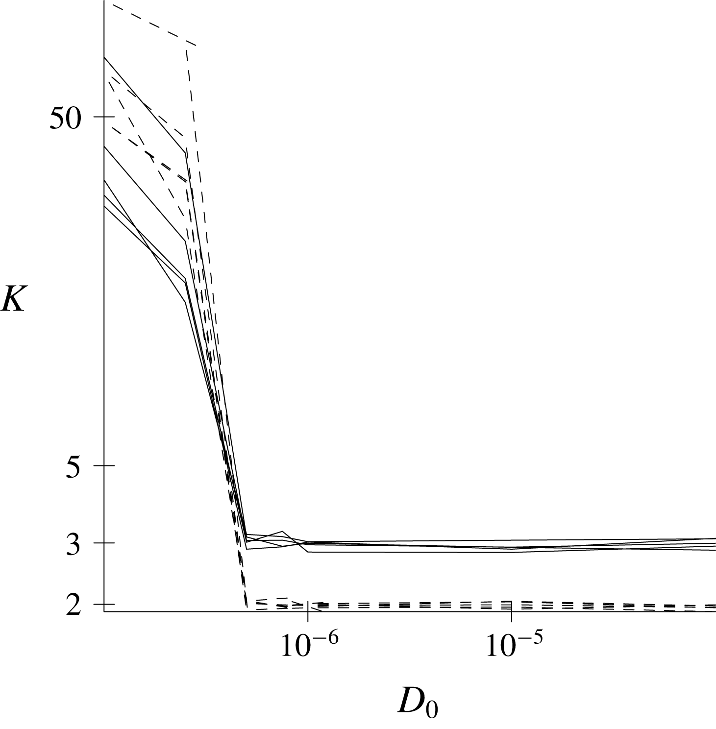
Figure 1. The vorticity kurtosis $K_{\unicode[STIX]{x1D701}}$ (solid lines) and strain kurtosis $K_{\unicode[STIX]{x1D70E}}$ (dashed lines) in four Monte Carlo computations in which the parameter $D_{0}$ is reduced, in stages, from $D_{0}=10^{-4}$ to $10^{-7}$ . The lighter lines correspond to the four separate computations, which differ only in the sequence of random numbers used in the computation. The two heavier lines represent the average of the four computations. The appearance of flow structures is associated with the rapid increase in the kurtoses that begins around $D_{0}=10^{-6}$ .

Figure 1 shows the vorticity kurtosis $K_{\unicode[STIX]{x1D701}}$ (solid lines) and strain kurtosis $K_{\unicode[STIX]{x1D70E}}$ (dashed lines) in four completely independent Monte Carlo computations in which $D_{0}$ is reduced, in stages, from $D_{0}=10^{-4}$ to $10^{-7}$ . The lighter lines correspond to the kurtosis values in the four calculations, and the heavier lines represent the average of the four. The four calculations differ only in the sequence of random numbers used by the Monte Carlo algorithm. Each of the four calculations terminates with $\unicode[STIX]{x1D713}(x,y)$ ‘frozen’ into a state exhibiting a small number of vorticity quadrupoles. These terminal states are shown in figures 2 and 3.

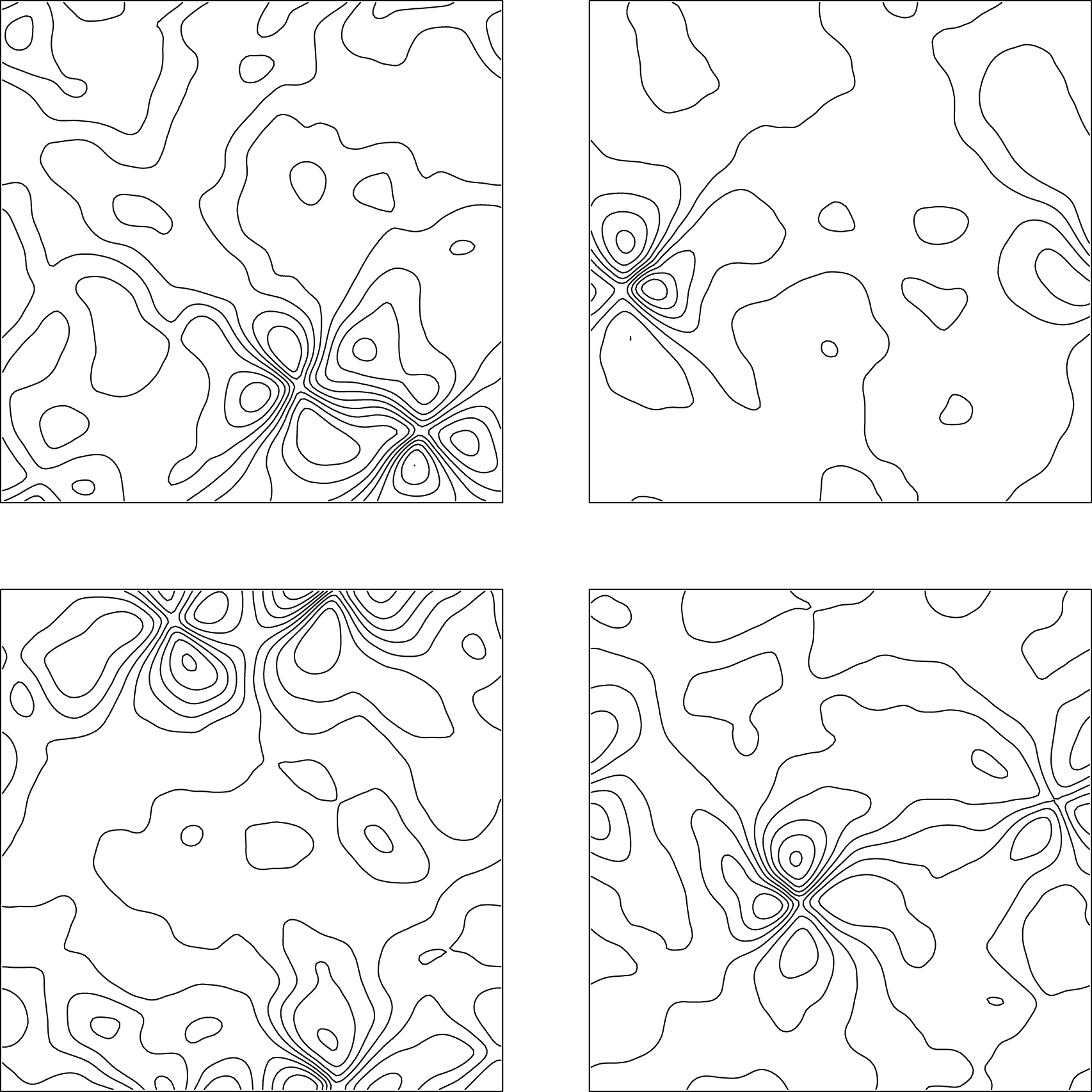
Figure 2. The stream function in the four independent Monte Carlo calculations at the value $D_{0}=10^{-7}$ . Heavier lines correspond to larger values of the stream function.

The appearance of the quadrupoles is associated with the increase in the kurtoses that begins around $D_{0}=10^{-6}$ . This is far below the $D_{0}=O(1)$ value stipulated by (2.20)–(2.21) for our choice of $\langle \unicode[STIX]{x1D701}^{2}\rangle =1$ . We note that (2.20)–(2.21) predict that $\unicode[STIX]{x1D707}(\boldsymbol{k})$ varies only logarithmically with $k$ in the enstrophy inertial range, where $E(k)\propto k^{-3}$ , and that our range of $k=1{-}64$ is relatively small. Thus, it is the size of $D_{0}$ and not its constancy that is unrealistic here. It can be shown that statistically independent, uniformly distributed phases correspond to $K_{\unicode[STIX]{x1D701}}=3$ and $K_{\unicode[STIX]{x1D70E}}=2$ . Figure 1 shows that these values persist right up until the rapid increase in the kurtoses that coincides with the appearance of the quadrupoles.

Figure 3. The vorticity corresponding to the stream function in figure 2.