


1. Introduction
The small-scale dynamics of turbulence can be described using the velocity gradient tensor, and is closely related to many important turbulent flow processes, including viscous dissipation of kinetic energy, enstrophy production and intermittency. There are numerous investigations on the statistical properties of the vorticity field, enstrophy transfer and strain-rate tensor for incompressible turbulent flows (Hamlington, Schumacher & Dahm Reference Hamlington, Schumacher and Dahm2008; Wallace Reference Wallace2009; Zhou et al. Reference Zhou, Nagata, Sakai, Ito and Hayase2016; Carter & Coletti Reference Carter and Coletti2018). Ashurst et al. (Reference Ashurst, Kerstein, Kerr and Gibson1987) pioneered numerical investigations of the alignments between vorticity and eigenvectors of the strain-rate tensor in incompressible isotropic turbulence and homogeneous shear turbulence. They found that the vorticity tends to align with the intermediate strain-rate eigenvector, and the strain-rate eigenvalues have a preferred ratio of  $-$4.0:1.0:3.0 in the highly dissipative region. Tsinober, Kit & Dracos (Reference Tsinober, Kit and Dracos1992) experimentally investigated the velocity gradients in both homogeneous and inhomogeneous incompressible turbulence based on the multi-hot-wire technique. Their results confirmed the strong tendency of alignment between the vorticity and the intermediate strain-rate eigenvector. Meanwhile, the preferred eigenvalue ratio was found to be
  $-$3.8:1.0:3.1, very close to
  $-$4.0:1.0:3.0. These behaviours were also observed in the later investigations for a wide variety of incompressible turbulent flows (Lüthi, Tsinober & Kinzelbach Reference Lüthi, Tsinober and Kinzelbach2005; Buaria, Bodenschatz & Pumir Reference Buaria, Bodenschatz and Pumir2020). More details about the velocity gradient tensor in incompressible turbulent flows can be found in the comprehensive review by Meneveau (Reference Meneveau2011).
Compared with incompressible turbulence, there are much fewer investigations on the vorticity field and strain-rate tensor in compressible turbulent flows. Erlebacher & Sarkar (Reference Erlebacher and Sarkar1993) numerically investigated the velocity gradient tensor in a weakly compressible homogeneous shear turbulence. A preferred strain-rate eigenvalue ratio of  $-$4.0:1.0:3.0 and the similar alignments between vorticity and strain-rate eigenvectors were observed as in incompressible flows. Their results revealed that the statistics of the velocity gradient tensor are not significantly modified by the local dilatation when the turbulent Mach number is smaller than 0.3. Furthermore, the most probable eigenvalue ratio for the dilatational component of deviatoric strain-rate tensor is found to be
  $-$2.2:1.0:1.2 in the strong compression region, indicating the dominant role of sheet-like structures in this region. Lee, Girimaji & Kerimo (Reference Lee, Girimaji and Kerimo2009) performed numerical simulations of decaying compressible isotropic turbulence with initial turbulent Mach numbers up to 0.885, wherein the strain-rate eigenvalue ratio of
  $-$4.0:1.0:3.0 and the alignments between vorticity and strain-rate eigenvectors still hold, although the preferential alignments are weakened in the strong compression region. One can expect that a stronger compression could show observable impacts. For example, in Wang et al. (Reference Wang, Shi, Wang, Xiao, He and Chen2012), with the turbulent Mach number is around 1.0, although the eigenvalue ratio of the solenoidal strain-rate tensor of approximately
  $-$3.7:1.0:2.7 is in good agreement with that in the incompressible turbulence, the eigenvalue ratio of the dilatational strain-rate tensor tends to be
  $-$1.0:0.0:0.0 in the high compression region, and the most probable eigenvalue ratio of the strain-rate tensor is approximately
  $-$3.0:1.0:2.5 in the overall flow field. They also found that the strong local compression motion enhances the enstrophy production, while the strong local expansion motion suppresses the enstrophy production by vortex stretching.
A general classification of local flow topology based on the three invariants of the velocity gradient tensor was proposed by Chong, Perry & Cantwell (Reference Chong, Perry and Cantwell1990). For incompressible turbulence, the first invariant (P) is null, and the local flow topology is fully characterized by the second (Q) and third (R) invariants. Extensive studies on the statistical properties in the Q–R plane have been performed numerically and experimentally (Nomura & Post Reference Nomura and Post1998; Nomura & Diamessis Reference Nomura and Diamessis2000; Bijlard et al. Reference Bijlard, Oliemans, Portela and Ooms2010). A universal teardrop shape of the joint probability density function (PDF) between the second and third invariants was observed for a wide variety of incompressible turbulent flows, including wall-bounded flows (Blackburn, Mansour & Cantwell Reference Blackburn, Mansour and Cantwell1996; Chong et al. Reference Chong, Soria, Perry, Chacin, Cantwell and Na1998), isotropic turbulence (Ooi et al. Reference Ooi, Martin, Soria and Chong1999) and the turbulence/non-turbulence interface in jets (da Silva & Pereira Reference da Silva and Pereira2008), etc.
Relevant investigations on the flow topology of compressible turbulence are relatively limited (Wang & Lu Reference Wang and Lu2012; Vaghefi & Madnia Reference Vaghefi and Madnia2015; Danish, Sinha & Srinivasan Reference Danish, Sinha and Srinivasan2016; Parashar, Sinha & Srinivasan Reference Parashar, Sinha and Srinivasan2019; Wang et al. Reference Wang, Wan, Chen, Xie, Zheng, Wang and Chen2020). Pirozzoli & Grasso (Reference Pirozzoli and Grasso2004) reported that the joint PDFs of the second and third invariants of the velocity gradient tensor in decaying compressible isotropic turbulence share a similar teardrop shape at various initial turbulent Mach numbers. Furthermore, the conditional average of the second invariant of the deviatoric strain-rate tensor with respect to the third one always scales with the 1/3 power of the discriminant of the velocity gradient tensor. Suman & Girimaji (Reference Suman and Girimaji2010) numerically investigated the local flow topology in compressible isotropic turbulence and analysed the dilatational effect on the flow topology. The investigation was based on the joint PDF of the second and third invariants of the velocity gradient tensor conditioned on the local dilatation. They showed that, at low dilatational levels, the local flow topology is similar to incompressible turbulence, while at high dilatational levels, the flow structures are significantly changed. At a higher turbulent Mach number of around 1.0 (Wang et al. Reference Wang, Shi, Wang, Xiao, He and Chen2012), in the compression region, the teardrop shape of the joint PDF exhibits a more extended tail in the fourth quadrant, which stems from the shocklet structures. In contrast, in the expansion region, the joint PDF takes a more rounded shape with a shortened bottom-right tail, and a nearly symmetric joint PDF appears in the strong expansion region.
In high-speed flows of practical interest, the hypersonic speed and/or the extreme levels of shear result in a high temperature in the shock layer and boundary layer (Candler Reference Candler2019). The vibrational non-equilibrium phenomenon resulting from the high temperature thus widely exists in the high-speed flows. The advent of vibrational relaxation has a profound impact on the flow dynamics (Fiévet & Raman Reference Fiévet and Raman2018; Knisely & Zhong Reference Knisely and Zhong2020), and renders the statistical properties of compressible turbulence more complicated. The investigations of the statistical properties of compressible isotropic turbulence in vibrational non-equilibrium were pioneered by Donzis & Maqui (Reference Donzis and Maqui2016), and followed by Khurshid & Donzis (Reference Khurshid and Donzis2019) and Zheng et al. (Reference Zheng, Wang, Noack, Li, Wan and Chen2020, Reference Zheng, Wang, Alam, Noack, Li, Wan and Chen2021). In our companion paper (Zheng et al. Reference Zheng, Wang, Alam, Noack, Li, Wan and Chen2021), we numerically simulated the statistically stationary compressible isotropic turbulence in vibrational non-equilibrium with a large-scale thermal forcing. It was revealed that the flow structures and compressibility are significantly modified due to the combined effects of vibrational relaxation and large-scale thermal forcing, especially for the cases with a turbulent Mach number of approximately 0.22. To our knowledge, the statistical properties of the small-scale structures of compressible isotropic turbulence in vibrational non-equilibrium have never been investigated systematically. In this work, we mainly focus on the combined impacts of vibrational relaxation and large-scale thermal forcing on the statistical properties of the strain-rate tensor, vorticity field, enstrophy production and flow topology. Such a comprehensive investigation would further deepen our understanding of small-scale features of compressible turbulence in vibrational non-equilibrium. The large amount of conditional statistics in current study will contribute to the development of accurate models for compressible turbulence in vibrational non-equilibrium.
The rest of paper is organized as follows. In § 2, the governing equations, thermodynamic and transport properties of compressible turbulence and a brief description of the numerical methodology will be introduced. The one-point statistics of the current simulated flows, including the statistical properties of the strain-rate components and vorticity, are given in § 3. The combined effects of vibrational relaxation and large-scale thermal forcing on the statistical properties of enstrophy production and flow topology are respectively presented in §§ 4 and 5. Finally, a discussion building the connection among various observations and the concluding remarks are provided in §§ 6 and 7.
2. Computational details
2.1. Governing equations and numerical method
In the current simulations, non-reactive mono-species gases and Newtonian fluids are considered, for which the dynamic viscosity relies only on the temperature. The dimensionless governing equations for compressible turbulence in vibrational non-equilibrium can be written as follows (Donzis & Maqui Reference Donzis and Maqui2016; Zheng et al. Reference Zheng, Wang, Alam, Noack, Li, Wan and Chen2021):
 \begin{gather} \frac{\partial {\rho}}{\partial {t}} + \frac{\partial(\rho u_j)}{\partial x_j} = 0 \end{gather}
 \begin{gather}\frac{\partial{(\rho u_i)}}{\partial {t}} + \frac{\partial{[\rho u_i u_j + p {\boldsymbol{\delta}}_{ij}]}}{\partial{x_j}} = \frac{1}{Re} \frac{\partial{\sigma_{ij}}}{\partial{x_j}} + \mathcal{F}_i \end{gather}
 \begin{gather}\frac{\partial{\varepsilon}}{\partial{t}} + \frac{\partial{[(\varepsilon + p)u_j]}}{\partial{x_j}}= \frac{1}{\alpha} \frac{\partial}{\partial{x_j}}\left(\kappa_{tr} \frac{\partial{T_{tr}}}{\partial{x_j}} + \kappa_v \frac{\partial{T_v}}{\partial{x_j}} \right) + \frac{1}{Re}\frac{\partial{(\sigma_{ij}u_i)}}{\partial{x_j}} - \varLambda + \mathcal{F}_I + \mathcal{F}_ju_j \end{gather}
 \begin{gather}\frac{\partial{E_v}}{\partial{t}} + \frac{\partial{(E_vu_j)}}{\partial{x_j}} = \frac{1}{\alpha} \frac{\partial}{\partial{x_j}}\left(\kappa_v \frac{\partial{T_v}}{\partial{x_j}}\right) + \frac{E_v^*-E_v}{\tau_v} \end{gather}
 \begin{gather}p = \rho T_{tr}/(\gamma_r M^2) \end{gather}
where  $\rho$,
  $u_i$,
  $p$,
$p$,  $T_{tr}$ and
  $T_v$ are the dimensionless density, velocity components, pressure, translational–rotational and vibrational temperatures, respectively. The total energy
  $\varepsilon$ includes the kinetic energy (
 $\rho u_j u_j /2$), and the translational–rotational (
 $E_{tr} = 5\rho T_{tr}/(2\gamma _r M^2)$) and vibrational (
 $E_v$) energies. The dimensionless, large-scale forcings to the fluid momentum and the translational–rotational energy are respectively denoted as
  $\mathcal {F}_j$ and
  $\mathcal {F}_I$, which are explained in more detail in the appendix of Zheng et al. (Reference Zheng, Wang, Alam, Noack, Li, Wan and Chen2021). A spatially uniform thermal cooling function
  $\varLambda$ is adopted to sustain the internal energy in a statistically steady state. In the equation of state (2.5), only the translational–rotational temperature
  $T_{tr}$ is adopted since the pressure mainly stems from the translational motion of molecules rather than the rotational and vibrational motions (Vincenti & Kruger Reference Vincenti and Kruger1965). The reference Reynolds number
  $Re = \rho _r U_r L_r/\mu _r$, the reference Mach number
  $M = U_r/c_r$ and the reference Prandtl number
  $Pr = \mu _r C_{p_r}/\kappa _r$ are three governing parameters. Here,
  $\rho _r$,
  $U_r$,
  $L_r$ and
  $\mu _r$ are respectively the reference density, velocity, length and viscosity coefficient. The reference speed of sound is given by
  $c_r = \sqrt {\gamma _r R T_r}$, where
  $R$ is the specific gas constant and
  $T_r = 1200$ K is the reference temperature. The parameter
  $\gamma _r = C_{p_r}/C_{v_r}$ is the ratio of specific heat at constant pressure
  $C_{p_r}$ to that at constant volume
  $C_{v_r}$, approximately equalling 1.324 according to the ratio of specific heats of dry air at
  $T_r = 1200$ K. The dimensionless parameter
  $\alpha$ is defined as
  $\alpha \equiv PrRe(\gamma _r-1)M^2$, where
  $Pr$ equals 0.71.
The vibrational energy per unit volume in equilibrium ( $E_v^*$) and non-equilibrium (
 $E_v$) for diatomic molecules, and the viscosity stress
  $\sigma _{ij}$ are given as
 \begin{gather} E_{v}^* = \frac{\rho \theta_{v}}{\gamma_r M^2 [\exp(\theta_{v}/T_{tr}) -1]}, \end{gather}
 \begin{gather}E_{v} = \frac{\rho \theta_{v}}{\gamma_r M^2 [\exp(\theta_{v}/T_v) -1]}, \end{gather}
and
 \begin{equation} \sigma_{ij} = \mu \left(\frac{\partial{u_i}}{\partial{x_j}} + \frac{\partial{u_j}}{\partial{x_i}}\right) - \frac{2}{3}\mu\theta{\boldsymbol{\delta}}_{ij}. \end{equation}
The parameter  $\theta _v$ is the characteristic vibrational temperature normalized by
  $T_r$, while
  $\theta = \partial u_k/\partial x_k$ is the velocity divergence. The temperature-dependent viscosity (
 $\mu$) and thermal conductivity coefficients (
 $\kappa _{tr}$ and
  $\kappa _{v}$) are specified by the Sutherland and Eucken laws (Vincenti & Kruger Reference Vincenti and Kruger1965; Anderson Reference Anderson2006). For their detailed expressions, please refer to our previous publication (Zheng et al. Reference Zheng, Wang, Noack, Li, Wan and Chen2020).
The vibrational rate  $Q_v = (E_v^*-E_v)/\tau _v$ in the vibrational energy governing equation (2.4) is based on the widely used Landau–Teller relaxation model. The dimensionless relaxation time (
 $\tau _v$) relies closely on the local temperature and pressure, and is roughly calculated by
 \begin{equation} \tau_v = (C/p)\exp(K_2/T_{tr})^{1/3}. \end{equation}
Here,  $C$ and
  $K_2$ are dimensionless constants relating to the molecular structure of gases. In the current simulations, the dimensionless parameter
  $\langle K_\tau \rangle = \langle \tau _v \rangle /\tau _\eta$ is adopted to characterize the time scale of the relaxation process, where the
  $\langle\, {\cdot }\, \rangle$ operator stands for the spatial average. Also,
  $\tau _\eta = [\langle \mu /(Re\rho )\rangle /\epsilon ]^{1/2}$ is the Kolmogorov time scale, and
  $\epsilon =\langle \sigma _{ij}{\mathsf{S}}_{ij}/Re \rangle / \langle \rho \rangle$ is the kinetic energy dissipation rate due to viscosity. The value of
  $K_2$ is set to be 2000.0, while the constant
  $C$ is adjusted to obtain a specific
  $\langle K_\tau \rangle$ value.
The governing equations of compressible turbulence are numerically solved in a cubic box with a side length equalling  $2{\rm \pi}$ and a
  $512^3$ grid resolution. Periodic boundary conditions are adopted in all three spatial directions. The hybrid compact-weighted essentially non-oscillatory (compact-WENO) scheme is applied, which couples a eighth-order central compact finite difference scheme in smooth regions with a seventh-order WENO scheme in shock regions (Lele Reference Lele1992; Balsara & Shu Reference Balsara and Shu2000; Wang et al. Reference Wang, Wang, Xiao, Shi and Chen2010). The time derivative is approximated by the total variation diminishing (TVD) Runge–Kutta method (Gottlieb & Shu Reference Gottlieb and Shu1998). Following Samtaney, Pullin & Kosović (Reference Samtaney, Pullin and Kosović2001), the velocity field, which is divergence free, is initialized using a random field with a specified spectrum (
 $E(k) = 0.011 k^4 \exp (-k^2/8)$, where
  $k$ is the wavenumber). Meanwhile, the normalized temperatures (
 $T_{tr}$ and
  $T_v$) and density (
 $\rho$) are initialized with constant values (1.0) at all spatial points, and the initial pressure is determined from the equation of state (2.5). After the system reaches the statistically stationary state, 61 flow fields, uniformly spanning the time period of
  $9.01 \lesssim t/T_e \lesssim 14.41$, are adopted to obtain the statistical averages of quantities. Here,
  $T_e (= \sqrt {3}L_f/u^\prime )$ is the large eddy turnover time and
  $L_f$ is the integral length scale.
2.2. Forcing strategy
The velocity field  ${\boldsymbol {u}}({\boldsymbol {x}},t)$ is transformed into the wave space using the Fourier transform, and further decomposed into a solenoidal field (
 $\hat {{\boldsymbol {u}}}^S({\boldsymbol {k}},t)$) and a dilatational field (
 $\hat {{\boldsymbol {u}}}^D({\boldsymbol {k}},t)$) based on the Helmholtz decomposition, where
  ${\boldsymbol {k}}$ is the wave vector. The kinetic energy per unit mass for each wave vector is thus decomposed as follows:
 \begin{equation} \frac{|\hat{{\boldsymbol{u}}}({\boldsymbol{k}},t)|^2}{2}= \frac{|\hat{{\boldsymbol{u}}}^S({\boldsymbol{k}},t)|^2}{2}+ \frac{|\hat{{\boldsymbol{u}}}^D({\boldsymbol{k}},t)|^2}{2}. \end{equation}
The kinetic energy in each of the first two wavenumber shells is calculated as
 \begin{equation} E^u(0.5 \leq k < 1.5) = \sum_{0.5 \leq | {\boldsymbol{k}} | < 1.5} \left(\frac{|\hat{{\boldsymbol{u}}}({\boldsymbol{k}},t)|^2}{2}\right), \end{equation}
and
 \begin{equation} E^u(1.5 \leq k < 2.5) = \sum_{1.5 \leq | {\boldsymbol{k}} | < 2.5}\left(\frac{|\hat{{\boldsymbol{u}}}({\boldsymbol{k}},t)|^2}{2}\right). \end{equation}
Similarly, the kinetic energy in the first two wavenumber shells is decomposed as
 \begin{equation} E^u(0.5 \leq k < 1.5) = E^{u,S}(0.5 \leq k < 1.5)+E^{u,D}(0.5 \leq k < 1.5), \end{equation}
and
 \begin{equation} E^u(1.5 \leq k < 2.5) = E^{u,S}(1.5\leq k < 2.5)+E^{u,D}(1.5\leq k < 2.5). \end{equation}
 The large-scale momentum forcing is applied to the solenoidal velocity component, while the dilatational velocity component is left untouched (Petersen & Livescu Reference Petersen and Livescu2010; Wang et al. Reference Wang, Wang, Xiao, Shi and Chen2010; Donzis & Jagannathan Reference Donzis and Jagannathan2013). To maintain the total kinetic energy in the first two shells to the prescribed levels  $E_u(1)$ and
  $E_u(2)$, respectively, the solenoidal velocity component is amplified. The forced velocity field
  $\hat {{\boldsymbol {u}}}^f({\boldsymbol {k}},t)$ is given as
 \begin{equation} \hat{{\boldsymbol{u}}}^f({\boldsymbol{k}},t)=\alpha \hat{{\boldsymbol{u}}}^S({\boldsymbol{k}},t)+\hat{{\boldsymbol{u}}}^D({\boldsymbol{k}},t), \end{equation}
where  $\alpha$ for all modes in each wavenumber shell is set to be
 \begin{equation} \alpha(0.5 \leq k < 1.5) = \sqrt{\frac{E^u(1)-E^{u,D}(0.5 \leq k < 1.5)}{E^{u,S}(0.5 \leq k < 1.5)}}, \end{equation}
and
 \begin{equation} \alpha(1.5 \leq k < 2.5) = \sqrt{\frac{E^u(2)-E^{u,D}(1.5\leq k < 2.5)}{E^{u,S}(1.5\leq k < 2.5)}}, \end{equation}
where  $E^u(1) = 1.242$ and
  $E^u(2) = 0.391$.
The large-scale thermal forcing for the translational–rotational temperature field is similar to that for the solenoidal velocity field (Donzis & Maqui Reference Donzis and Maqui2016; Wang et al. Reference Wang, Wan, Chen, Xie, Wang and Chen2019). The translational–rotational temperature field  $T_{tr}({\boldsymbol {x}},t)$ is transformed into Fourier space to yield
  $\hat {T}_{tr}({\boldsymbol {k}},t)$. Similarly,
 \begin{equation} E^{T_{tr}}(0.5 \leq k < 1.5) = \sum_{0.5 \leq | {\boldsymbol{k}} | < 1.5} (|\hat{T}_{tr}({\boldsymbol{k}},t)|^2), \end{equation}
and
 \begin{equation} E^{T_{tr}}(1.5 \leq k < 2.5) = \sum_{1.5 \leq | {\boldsymbol{k}} | < 2.5} (|\hat{T}_{tr}({\boldsymbol{k}},t)|^2). \end{equation}
The forced translational–rotational temperature is given as
 \begin{equation} \hat{T}_{tr}^f({\boldsymbol{k}},t) = \beta \hat{T}_{tr}({\boldsymbol{k}},t), \end{equation}
where  $\beta$ for all modes in each wavenumber shell is set to be
 \begin{equation} \beta(0.5 \leq k < 1.5) = \sqrt{\frac{E^{T_{tr}}(1)}{{E^{T_{tr}}(0.5 \leq k < 1.5)}}}, \end{equation}
and
 \begin{equation} \beta(1.5 \leq k < 2.5) = \sqrt{\frac{E^{T_{tr}}(2)}{{E^{T_{tr}}(1.5 \leq k < 2.5)}}}, \end{equation}
where  $E^{T_{tr}}(1) = E^u(1)/100$ and
  $E^{T_{tr}}(2) = E^u(2)/100$.
In present simulations, the momentum and thermal forcings act on the large scales, and are expected to have a small impact on the statistics properties in the inertial regime. However, the large-scale thermal forcing in the present simulations cannot completely reproduce the shock-induced heating in the high-speed flows of practical interest.
3. Simulation parameters and one-point statistics
The overall statistics for the current simulations are summarized in tables 1–4. The reference Reynolds number ( $Re$) equals 400, and the reference Mach numbers (
 $M$) are set to be 0.099 and 0.296. Three characteristic vibrational temperatures (
 $\theta _v$ = 1.0, 3.0 and 5.0) are employed. A smaller
  $\theta _v$ suggests an easier excitation for the vibrational mode. The spatially averaged ratio of the vibrational energy to the total internal energy (i.e.
  $\langle E_v^*/(E_{tr}+E_v^*) \rangle$) approximately equals 18.88 %, 5.92 % and 1.34 % with
  $\theta _v = 1.0$, 3.0 and 5.0, respectively. The Taylor microscale Reynolds number (
 $Re_\lambda$) and turbulent Mach number (
 $M_t$) are respectively defined as
 \begin{equation} Re_\lambda = Re\frac{\langle \rho \rangle u^\prime \lambda}{\sqrt{3}\langle \mu \rangle},\quad \textrm{and} \quad M_t = M\frac{u^\prime}{\langle \sqrt{T_{tr}} \rangle}, \end{equation}
where the root mean square (r.m.s.) value of velocity magnitude ( $u^\prime$) and the Taylor microscale (
 $\lambda$) are respectively given as
 \begin{equation} u^\prime = \sqrt{\langle u_1^2 + u_2^2 + u_3^2 \rangle}, \end{equation}
and
 \begin{equation} \lambda = \sqrt {\frac{\langle u_1^2 + u_2^2 + u_3^2 \rangle}{\langle (\partial{u_1}/\partial{x_1})^2 + (\partial{u_2}/\partial{x_2})^2 + (\partial{u_3}/\partial{x_3})^2\rangle}}. \end{equation}
Table 1. Simulation parameters and resulting flow statistics for compressible turbulence with  $M_t \approx 0.22$. Considering effects of
  $\langle K_\tau \rangle$.

Here,  $M_t$ roughly equals
  $0.22$ and
  $0.68$ for the
  $M = 0.099$ and
  $0.296$ cases, respectively, while
  $Re_\lambda$ is approximately
  $157.5$ (tables 1–4). The value of
  $\langle K_\tau \rangle$ approximately equals 0.16–741.4 for the
  $M = 0.099$ cases, and 0.19–931.0 for the
  $M = 0.296$ cases. In the present simulations, cases
  $\textrm {I}_1\unicode{x2013}\textrm {I}_5$ and
  $\textrm {II}_1\unicode{x2013}\textrm {II}_5$ are used to discuss the effect of
  $\langle K_\tau \rangle$, while cases
  $\textrm {I}_2$,
  $\textrm {I}_6$,
  $\textrm {I}_7$ and cases
  $\textrm {II}_2$,
  $\textrm {II}_6$,
  $\textrm {II}_7$ are adopted to study the effect of
  $\theta _v$. Note that cases
  $\textrm {I}_5$ and
  $\textrm {II}_5$ can be approximately treated as frozen flow (Knisely & Zhong Reference Knisely and Zhong2020) since their vibrational relaxation times are significantly larger than the Kolmogorov time scale (i.e.
  $\langle K_\tau \rangle \gg 1.0$). In the tables of this article, cases
  $\textrm {I}_3$,
  $\textrm {I}_5$ and
  $\textrm {I}_7$, as well as cases
  $\textrm {II}_3$,
  $\textrm {II}_5$ and
  $\textrm {II}_7$, are marked with colours as typical cases for easy comparison.
As presented in tables 1–4, the resolution parameter  $\eta /{\rm \Delta} x$ is in the range of
 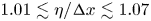 $1.01 \lesssim \eta / {\rm \Delta} x \lesssim 1.07$, where
  $\eta$ is the Kolmogorov length scale and
  ${\rm \Delta} x$ is the grid spacing in each direction. The resolution parameter
  $k_{max}\eta$ is therefore in the range of
  $3.18 \lesssim k_{max}\eta \lesssim 3.37$, where the largest wavenumber
  $k_{max}$ is half of the number of grid points in each direction. According to previous grid refinement studies (Wang et al. Reference Wang, Shi, Wang, Xiao, He and Chen2011, Reference Wang, Shi, Wang, Xiao, He and Chen2012), the grid resolutions with
  $k_{max}\eta \geq 2.77$ is enough for the convergence of the flow statistics.
The r.m.s. value of the velocity divergence ( $\theta ^\prime$) is used to characterize the flow compressibility. The greater the
  $\theta ^\prime$, the stronger the flow compressibility. For the
  $M_t \approx 0.22$ cases (tables 1–2),
  $\theta ^\prime$ decreases from 0.91 to 0.56 as
  $\langle K_\tau \rangle$ increases from 0.16 to 4.00, and sharply increases to 3.63 with
  $\langle K_\tau \rangle \approx 741.4$;
  $\theta ^\prime$ increases from 0.58 to 1.78 with
  $\theta _v$ varying from 1.0 to 5.0. Similarly, for the
  $M_t \approx 0.68$ cases (tables 3–4),
  $\theta ^\prime$ decreases from 2.50 to 1.67 as
  $\langle K_\tau \rangle$ increases from 0.19 to 4.27, and increases to 3.40 with
  $\langle K_\tau \rangle \approx 931.0$;
  $\theta ^\prime$ increases from 2.10 to 2.95 with
  $\theta _v$ varying from 1.0 to 5.0. As revealed in Zheng et al. (Reference Zheng, Wang, Alam, Noack, Li, Wan and Chen2021), the large-scale thermal forcing enhances the flow compressibility, while the vibrational relaxation weakens it. From tables 1–4, cases
  $\textrm {I}_3$ and
  $\textrm {II}_3$ have the weakest compressibility, which suggests that they have the strongest relaxation level.
Table 2. Simulation parameters and resulting flow statistics for compressible turbulence with  $M_t \approx 0.22$. Considering effects of
  $\theta _v$.

Table 3. Simulation parameters and resulting flow statistics for compressible turbulence with  $M_t \approx 0.68$. Considering effects of
  $\langle K_\tau \rangle$.

Table 4. Simulation parameters and resulting flow statistics for compressible turbulence with  $M_t \approx 0.68$. Considering effects of
  $\theta _v$.

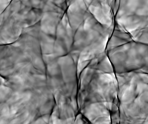
The instantaneous contours of  $\theta /\theta ^\prime$ with four typical cases (
 $\mathrm {I}_3$,
  $\mathrm {I}_5$,
  $\mathrm {II}_3$ and
  $\mathrm {II}_5$) in figure 1 and the PDFs of
  $\theta /\theta ^\prime$ in figure 2 show a balance between the vibrational relaxation and the large-scale thermal forcing. One can see consistent results with tables 1–4. For the
  $M_t \approx 0.22$ cases, when the relaxation effect is significant (e.g. case
  $\mathrm {I}_3$), the large-scale thermal forcing cannot strongly enhance the flow compressibility; no clear shocklet structure can be observed in the flow field (figure 1a) and the PDF of
  $\theta /\theta ^\prime$ is almost symmetrical about the
  $\theta /\theta ^\prime = 0.0$ axis (figure 2a). As the relaxation effect fades (e.g. case
  $\mathrm {I}_5$), the large-scale thermal forcing significantly enhances the flow compressibility; the clear shocklet structures lie across the flow field (figure 1b), and the PDF of
  $\theta /\theta ^\prime$ is thus strongly skewed to the negative side (figure 2a). However, in comparison with the
  $M_t \approx 0.22$ cases, the large-scale thermal forcing and vibration relaxation have a weaker impact on the flow compressibility for the
  $M_t \approx 0.68$ cases, although similar phenomena are observed. The flow compressibility for case
  $\mathrm {II}_5$ is obviously stronger than that of case
  $\mathrm {II}_3$. For case
  $\mathrm {II}_5$, the shocklet structures are more clear (figure 1c,d) and there is a stronger tendency for the PDF of
  $\theta /\theta ^\prime$ to be skewed to a negative value (figure 2b). In order to clarify possible similarities to incompressible turbulence, the component of the strain tensor
  ${\mathsf{S}}_{ij}$ (
 $=(\partial u_i/\partial x_j+\partial u_j/\partial x_i)/2$) is separated into the deviatoric strain-rate term
  ${\mathsf{D}}_{ij}\ (= {\mathsf{S}}_{ij}-{\mathsf{S}}_{kk}{\boldsymbol{\delta}}_{ij}/3)$ and the isotropic dilatational term
  $-{\mathsf{S}}_{kk}{\boldsymbol{\delta}}_{ij}/3$ (Erlebacher & Sarkar Reference Erlebacher and Sarkar1993). Based on the Helmholtz decomposition,
  ${\mathsf{D}}_{ij}$ can be further decomposed into the solenoidal and dilatational components, i.e.
  ${\mathsf{D}}_{ij} = {\mathsf{D}}^S_{ij} + {\mathsf{D}}^D_{ij}$, where
  ${\mathsf{D}}^S_{ij}=(\partial u^S_i/\partial x_j+\partial u^S_j/\partial x_i)/2$ and
  ${\mathsf{D}}^D_{ij}=(\partial u^D_i/\partial x_j+\partial u^D_j/\partial x_i)/2 - \theta {\boldsymbol{\delta}}_{ij}/3$. The solenoidal velocity component
  $\boldsymbol {u}^S$ satisfies
  $\boldsymbol {\nabla }\boldsymbol {\cdot} \boldsymbol {u}^S = 0$, while the dilatational velocity component
  $\boldsymbol {u}^D$ follows
  $\boldsymbol {\nabla } \times \boldsymbol {u}^D = 0$.

Figure 1. Instantaneous contours of normalized dilatation ( $\theta /\theta ^\prime$). (a) Case
  $\mathrm {I}_3$, (b) case
  $\mathrm {I}_5$, (c) case
  $\mathrm {II}_3$, (d) case
  $\mathrm {II}_5$. Here, x = 3.14.

Figure 2. PDFs of normalized dilatation for the (a)  $M_t \approx 0.22$ and (b)
  $M_t \approx 0.68$ cases.
As shown in tables 1–4, the dependence of  $\langle {\mathsf{D}}_{ij}^D{\mathsf{D}}_{ij}^D \rangle$ on the vibrational relaxation behaves quite similar to
  $\theta ^\prime$, being smaller when the relaxation effect is significant (i.e. cases
  $\textrm {I}_3$ and
  $\textrm {II}_3$). For instance,
  $\langle {\mathsf{D}}_{ij}^D {\mathsf{D}}_{ij}^D \rangle$ decreases from 0.55 to 0.22 as
  $\langle K_\tau \rangle$ increases from 0.16 to 4.00, and jumps to 8.80 with
  $\langle K_\tau \rangle \approx 741.4$ (
 $M_t \approx 0.22$ cases, table 1). Similarly, variations of
  $\langle \omega ^2 \rangle$ and
  $\langle {\mathsf{D}}_{ij}^S{\mathsf{D}}_{ij}^S \rangle$ are consistent with each other. Here, the vorticity is defined as
  ${\boldsymbol{\omega} = \boldsymbol {\nabla} \times \boldsymbol {u}}$ and
  $\langle \omega ^2 \rangle = \langle \omega _1^2 + \omega _2^2 + \omega _3^2 \rangle$. However, the variation of
  $\langle \omega ^2 \rangle$ (or
  $\langle {\mathsf{D}}_{ij}^S{\mathsf{D}}_{ij}^S \rangle$) is independent of the dilatation and vibrational relaxation.
Erlebacher & Sarkar (Reference Erlebacher and Sarkar1993) mentioned that, in compressible homogeneous turbulence, the dilatation is statistically independent of the vorticity and variables constructed from the solenoidal velocity component. The statistical correlation between two parameters (i.e. f and g) can be estimated by their correlation coefficient
 \begin{equation} \textrm{Corr}(f, g) = \frac{\langle (f-\langle f \rangle)(g-\langle g \rangle) \rangle }{\sqrt{\langle (f-\langle f \rangle)^2 \rangle\langle (g-\langle g \rangle)^2\rangle}}. \end{equation}
The corresponding correlation coefficients for the  $M_t \approx 0.22$ and
  $M_t \approx 0.68$ cases are given in tables 5 and 6. For the
  $M_t \approx 0.22$ cases (table 5), the small
  $\textrm {Corr}(\theta ^2, \omega ^2)$,
  $\textrm {Corr}(\theta ^2, {\mathsf{D}}_{ij}^S{\mathsf{D}}_{ij}^S)$ and
  $\textrm {Corr}(\omega ^2, {\mathsf{D}}_{ij}^D{\mathsf{D}}_{ij}^D)$ for different cases (
 ${<}0.14$) suggest a weak correlation between the dilatation and the vorticity or the solenoidal component of the deviatoric strain-rate tensor, as well as that between the vorticity and the dilatational component of the deviatoric strain-rate tensor. However, for cases with a significant relaxation effect (i.e. cases
  $\textrm {I}_1\unicode{x2013}\textrm {I}_3$, especially case
  $\textrm {I}_3$), the correlation coefficients are larger than the other cases. For compressible turbulence without considering the relaxation effect, the correlation coefficients between the dilatation and any variables constructed from the solenoidal velocity component are less than 0.01 (Erlebacher & Sarkar Reference Erlebacher and Sarkar1993). However, in the current simulations,
  $\textrm {Corr}(\theta ^2, {\mathsf{D}}_{ij}^S{\mathsf{D}}_{ij}^S) \approx 0.137$ for case
  $\textrm {I}_3$, suggesting that the correlation between the dilatation and the solenoidal component of the deviatoric strain-rate tensor is enhanced by the relaxation effect. Similarly, the relaxation effect weakens the correlation between the dilatation and the dilatational component of the deviatoric strain-rate tensor. The value of
  $\textrm {Corr}(\theta ^2, {\mathsf{D}}_{ij}^D{\mathsf{D}}_{ij}^D) \approx 0.662$ with
  $\langle K_\tau \rangle \approx 0.16$, and sharply reduces to 0.285 with
  $\langle K_\tau \rangle \approx 4.00$. For cases
  $\textrm {I}_4 \unicode{x2013}\textrm {I}_7$, where the relaxation effect fades,
  $\textrm {Corr}(\theta ^2, {\mathsf{D}}_{ij}^D{\mathsf{D}}_{ij}^D) \approx 0.943$. Interestingly,
  $\textrm {Corr}(\omega ^2, {\mathsf{D}}_{ij}^S{\mathsf{D}}_{ij}^S)$ is almost not affected by the vibrational relaxation,
  ${\approx }0.528$ (table 5).
Table 5. Correlation coefficients between some pairs of variables;  $M_t \approx 0.22$.

Table 6. Correlation coefficients between some pairs of variables;  $M_t \approx 0.68$.

For the  $M_t \approx 0.68$ cases (table 6),
  $\textrm {Corr}(\theta ^2, \omega ^2) \approx \textrm {Corr}(\theta ^2, {\mathsf{D}}_{ij}^S{\mathsf{D}}_{ij}^S) \approx 0.012$, indicating that the dilatation is nearly uncorrelated with the vorticity and the solenoidal component of the deviatoric strain-rate tensor. Similarly,
  $\textrm {Corr}(\omega ^2, {\mathsf{D}}_{ij}^D{\mathsf{D}}_{ij}^D) \approx 0.034$. However,
  $\theta ^2$ (or
  $\omega ^2$) strongly correlates with
  ${\mathsf{D}}_{ij}^D{\mathsf{D}}_{ij}^D$ (or
  ${\mathsf{D}}_{ij}^S{\mathsf{D}}_{ij}^S$), where
  $\textrm {Corr}(\theta ^2, {\mathsf{D}}_{ij}^D{\mathsf{D}}_{ij}^D) \approx 0.924$ and
 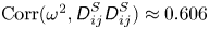 $\textrm {Corr}(\omega ^2, {\mathsf{D}}_{ij}^S{\mathsf{D}}_{ij}^S) \approx 0.606$. Furthermore, the correlation between the dilatation (or vorticity) and the dilatational (or solenoidal) component of the deviatoric strain-rate tensor is nearly not affected by the vibrational relaxation (table 6). To quantify the effects of dilatation, the flow region is divided into six subregions based on the local dilatational level: (i) strong compression region with
  $\theta / \theta ^\prime \in (-\infty, -2.0]$; (ii) moderate compression region with
  $\theta / \theta ^\prime \in ( -2.0, -1.0]$; (iii) weak compression region with
  $\theta / \theta ^\prime \in (-1.0, 0.0]$; (iv) weak expansion region with
  $\theta / \theta ^\prime \in (0.0, 1.0]$; (v) moderate expansion region with
  $\theta / \theta ^\prime \in (1.0, 2.0]$; (vi) strong expansion region with
  $\theta / \theta ^\prime \in (2.0, +\infty )$. Figure 3 presents the averages of the normalized magnitude of the vorticity and deviatoric strain-rate components conditioned on the local dilatation. For the
  $M_t \approx 0.22$ cases, conditional averages of
  $\omega ^2/\langle \omega ^2\rangle$ and
  ${\mathsf{D}}_{ij}^S{\mathsf{D}}_{ij}^S / \langle {\mathsf{D}}_{ij}^S{\mathsf{D}}_{ij}^S \rangle$ have similar behaviours (figure 3a,b). When the relaxation effect is significant (e.g. cases
  $\textrm {I}_1\unicode{x2013}\textrm {I}_3$), as revealed in table 5, the correlation between the dilatation and vorticity (as well as the solenoidal component of the deviatoric strain-rate tensor) is stronger than the other cases. Consequently, the conditional averages of
  $\omega ^2/\langle \omega ^2\rangle$ and
  ${\mathsf{D}}_{ij}^S{\mathsf{D}}_{ij}^S /\langle {\mathsf{D}}_{ij}^S{\mathsf{D}}_{ij}^S \rangle$ increase sharply in the strong expansion region. Similarly, they increase with the local dilatational level in the strong compression region. However, the growth rate for case
  $\textrm {I}_3$ is obviously larger than the other two cases. For the cases with a weak relaxation effect (e.g. cases
  $\textrm {I}_4\unicode{x2013}\textrm {I}_7$), the conditional averages of
  $\omega ^2/\langle \omega ^2\rangle$ and
  ${\mathsf{D}}_{ij}^S{\mathsf{D}}_{ij}^S / \langle {\mathsf{D}}_{ij}^S{\mathsf{D}}_{ij}^S \rangle$ approach 1.0 in the compression region, and increase slightly in the expansion region. In figure 3(c), the conditional average of
  ${\mathsf{D}}_{ij}^D{\mathsf{D}}_{ij}^D / \langle {\mathsf{D}}_{ij}^D{\mathsf{D}}_{ij}^D \rangle$ approaches zero at
  $\theta /\theta ^\prime = 0.0$, and increases with the local dilatational level in both compression and expansion regions. As the flow compressibility for cases
  $\textrm {I}_1\unicode{x2013}\textrm {I}_3$ is weakened by the relaxation effect, the conditional averages of
  ${\mathsf{D}}_{ij}^D{\mathsf{D}}_{ij}^D /\langle {\mathsf{D}}_{ij}^D{\mathsf{D}}_{ij}^D \rangle$ for these cases are thus smaller than other cases with identical dilatational levels. Note that, in figure 3(a–c), the lines fluctuate irregularly in the ranges of
  $\theta / \theta ^\prime < -5.0$ and
  $\theta / \theta ^\prime > 5.0$, especially for cases
  $\textrm {I}_1\unicode{x2013}\textrm {I}_3$. This observation can be attributed to the insufficient data in these ranges due to the weak dilatation, as shown in figure 2.

Figure 3. Conditional averages of the normalized magnitudes of the vorticity and deviatoric strain-rate components; (a,d)  $\langle \omega ^2 /\langle \omega ^2 \rangle \mid \theta /\theta ^\prime \rangle$, (b,e)
  $\langle {\mathsf{D}}_{ij}^S{\mathsf{D}}_{ij}^S / \langle {\mathsf{D}}_{ij}^S{\mathsf{D}}_{ij}^S \rangle \mid \theta /\theta ^\prime \rangle$ and (c,f)
  $\langle {\mathsf{D}}_{ij}^D{\mathsf{D}}_{ij}^D / \langle {\mathsf{D}}_{ij}^D{\mathsf{D}}_{ij}^D \rangle \mid \theta /\theta ^\prime \rangle$. For (a–c)
  $M_t \approx 0.22$ and (d–f)
  $M_t \approx 0.68$.
For the  $M_t \approx 0.68$ cases, the conditional averages of
  $\omega ^2/\langle \omega ^2\rangle$ and
  ${\mathsf{D}}_{ij}^S{\mathsf{D}}_{ij}^S / \langle {\mathsf{D}}_{ij}^S{\mathsf{D}}_{ij}^S \rangle$ are almost constant, being nearly independent of the local dilatation in the strong compression region (figure 3d,e). They decrease slightly in the range of
  $-2.0 \leq \theta /\theta ^\prime \leq 0.0$, and increase monotonically in the expansion region. Meanwhile, the conditional average of
  ${\mathsf{D}}_{ij}^D{\mathsf{D}}_{ij}^D / \langle {\mathsf{D}}_{ij}^D{\mathsf{D}}_{ij}^D \rangle$ rises with the local dilatation in both compression and expansion regions (figure 3f). Effects of vibrational relaxation on the conditional averages of
  $\omega ^2/\langle \omega ^2\rangle$,
  ${\mathsf{D}}_{ij}^D{\mathsf{D}}_{ij}^D / \langle {\mathsf{D}}_{ij}^D{\mathsf{D}}_{ij}^D \rangle$ and
  ${\mathsf{D}}_{ij}^S{\mathsf{D}}_{ij}^S / \langle {\mathsf{D}}_{ij}^S{\mathsf{D}}_{ij}^S \rangle$ are negligible; the lines corresponding to different cases almost overlap each other. These observations agree with the results in table 6.
4. Enstrophy production
4.1. Dilatational effect on enstrophy production
From the vorticity transport equation, the governing equation for enstrophy ( $\omega ^2/2$) can be derived as follows (Wang et al. Reference Wang, Shi, Wang, Xiao, He and Chen2011; Papapostolou et al. Reference Papapostolou, Wacks, Chakraborty, Klein and Im2017):
 \begin{align} \left(\frac{\partial}{\partial t}+u_j\frac{\partial}{\partial x_j} \right) \frac{\omega^2}{2} &= \omega _i \omega _j {\mathsf{S}}_{ij}- \omega ^2\theta + \omega _i\frac{\epsilon _{ijk}}{\rho ^2}\frac{\partial \rho}{\partial x_j} \frac{\partial p}{\partial x_k} \nonumber\\ &\quad +\omega _i \frac{\epsilon _{ijk}}{Re} \frac{\partial}{\partial x_j}\left(\frac{1}{\rho}\frac{\partial \sigma_{mk}}{\partial x_m} \right) + \omega_i \epsilon _{ijk} \frac{\partial \mathcal{F}_k}{\partial x_j}. \end{align}
 In (4.1),  $P_\omega = \omega _i \omega _j {\mathsf{S}}_{ij}$ is the vortex stretching and tilting (strain) term,
  $D_\omega = - \omega ^2\theta$ is the dilatational term,
  $B_\omega = (1/\rho ^2)\varepsilon _{ijk}\omega _i(\partial \rho / \partial x_j)(\partial p / \partial x_j)$ is the baroclinic term,
  $V_\omega = (1/Re)\omega _i \epsilon _{ijk}(\partial /\partial x_j)(\partial \sigma / \partial x_m)$ is the viscous term and
  $F_\omega = \omega _i \epsilon _{ijk}(\partial \mathcal {F}_k / \partial x_j)$ is the large-scale forcing term. The parameter
  $F_\omega$ is expected to have a small impact on the local enstrophy production because the momentum forcing is at large scales. The local enstrophy production thus mainly includes contributions from the strain, dilatational and baroclinic effects. However, the contribution from the baroclinic term is negligible in compressible isotropic turbulence (Wang et al. Reference Wang, Shi, Wang, Xiao, He and Chen2011). The specific focus in the current analysis is therefore on the strain and dilatational terms.
Equation (4.1) can be further derived as
 \begin{align} \frac{\partial (\omega ^2/2)}{\partial t}+\frac{\partial (u_j \omega ^2/2)}{\partial x_j}= \omega _i\omega _j {\mathsf{S}}^*_{ij}+\omega _i\frac{\epsilon _{ijk}}{\rho ^2}\frac{\partial \rho}{\partial x_j} \frac{\partial p}{\partial x_k}+\omega _i\frac{\epsilon _{ijk}}{Re}\frac{\partial}{\partial x_j} \left(\frac{1}{\rho}\frac{\partial \sigma _{mk}}{\partial x_m} \right) + \omega _i \epsilon _{ijk} \frac{\partial \mathcal{F}_k}{\partial x_j}, \end{align}
where the component of the modified strain-rate tensor  ${\mathsf{S}}^*_{ij}={\mathsf{S}}_{ij}-{\mathsf{S}}_{kk}{\boldsymbol{\delta}}_{ij}/2={\mathsf{D}}_{ij}-{\mathsf{S}}_{kk}{\boldsymbol{\delta}}_{ij}/6$. The net enstrophy production term (
 $\omega _i\omega _j {\mathsf{S}}^*_{ij}$) thus can be rewritten as
 \begin{equation} \omega_i\omega _j {\mathsf{S}}^*_{ij} = \omega_i\omega _j {\mathsf{D}}^S_{ij} + \omega_i\omega _j {\mathsf{D}}^D_{ij} - \frac{1}{6}\theta \omega ^2. \end{equation}
 The spatial averages of the net enstrophy production and its components for the  $M_t \approx 0.22$ and
  $0.68$ cases are listed in table 7. It is clearly observed that
  $\langle \omega _i\omega _j {\mathsf{S}}^*_{ij} \rangle \approx \langle \omega _i\omega _j {\mathsf{D}}^S_{ij} \rangle$, while
  $\langle \omega _i\omega _j {\mathsf{D}}^D_{ij} \rangle$ and
  $\langle -(1/6)\theta \omega ^2 \rangle$ are negligible. This indicates that, from the full flow field perspective, the enstrophy production mainly stems from the solenoidal component of the deviatoric strain-rate tensor. However, there is no obvious relationship between the spatial averages of the net enstrophy production (or its components) and the vibrational relaxation. Figure 4 illustrates the instantaneous contours of
  $\omega /\omega ^\prime$,
  $\omega _i \omega _j {\mathsf{D}}_{ij}^{S} /\langle \omega _i \omega _j {\mathsf{S}}_{ij}^* \rangle$,
  $\omega _i \omega _j {\mathsf{D}}_{ij}^{D} /\langle \omega _i \omega _j {\mathsf{S}}_{ij}^* \rangle$ and
  $-(1/6)\omega ^2\theta /\langle \omega _i \omega _j {\mathsf{S}}_{ij}^* \rangle$ for case
  $\mathrm {I}_5$. While the correlation coefficients between vorticity and different enstrophy production terms (including their absolute values) are listed in table 8. It is found that the structures of the vorticity (
 $\omega /\omega ^\prime$) and enstrophy production terms (
 $\omega _i \omega _j {\mathsf{D}}_{ij}^{S} /\langle \omega _i \omega _j {\mathsf{S}}_{ij}^* \rangle$,
  $\omega _i \omega _j {\mathsf{D}}_{ij}^{D} /\langle \omega _i \omega _j {\mathsf{S}}_{ij}^* \rangle$ and
  $-(1/6)\omega ^2\theta /\langle \omega _i \omega _j {\mathsf{S}}_{ij}^* \rangle$) are similar, for example, as marked by the circles with a dashed line. Consequently, the vorticity has a strong correlation with the absolute values of the enstrophy production terms. The correlation coefficients are larger than 0.53 (table 8). On the other hand, unlike the global averages in table 7, the local magnitudes of
  $\omega _i \omega _j {\mathsf{D}}_{ij}^{D} /\langle \omega _i \omega _j {\mathsf{S}}_{ij}^* \rangle$ and
  $-(1/6)\omega ^2\theta /\langle \omega _i \omega _j {\mathsf{S}}_{ij}^* \rangle$ can be considerable, especially for cases with a weak relaxation effect (e.g. case
  $\mathrm {I}_5$, figure 4c,d). However, the positive values in the compression region and the negative values in the expansion region cancel out on average, leading to a negligible amount. This is why
  $\textrm {Corr}(\omega /\omega ^\prime, \mathcal {W}({\mathsf{D}}^D_{ij}))$ and
  $\textrm {Corr}(\omega /\omega ^\prime, \mathcal {W}(-\theta /6))$ are close to zero (table 8).

Figure 4. Instantaneous contours of (a)  $\omega /\omega ^\prime$, (b)
  $\omega _i \omega _j {\mathsf{D}}_{ij}^{S} /\langle \omega _i \omega _j {\mathsf{S}}_{ij}^* \rangle$, (c)
  $\omega _i \omega _j {\mathsf{D}}_{ij}^{D} /\langle \omega _i \omega _j {\mathsf{S}}_{ij}^* \rangle$, (d)
  $-(1/6)\omega ^2\theta /\langle \omega _i \omega _j {\mathsf{S}}_{ij}^* \rangle$. Here, x = 3.14 and
  $\omega ^\prime = \sqrt {\langle \omega _1^2 + \omega _2^2 + \omega _3^2 \rangle }$. Case
  $\mathrm {I}_5$.
Table 7. Spatial averages of the net enstrophy production and its components;  $\mathcal {F}({\mathsf{S}}^*_{ij}) = \langle \omega _i \omega _j {\mathsf{S}}^*_{ij} \rangle$,
  $\mathcal {F}({\mathsf{D}}^S_{ij}) = \langle \omega _i \omega _j {\mathsf{D}}^S_{ij} \rangle$,
  $\mathcal {F}({\mathsf{D}}^D_{ij}) = \langle \omega _i \omega _j {\mathsf{D}}^D_{ij} \rangle$ and
  $\mathcal {F}(-\theta /6) = \langle -\omega ^2\theta /6 \rangle$.

Table 8. Correlation coefficients between vorticity and enstrophy production terms (including their absolute values). Case  $\mathrm {I}_5$;
  $\mathcal {W}({\mathsf{S}}^*_{ij}) = \omega _i \omega _j {\mathsf{S}}^*_{ij}/\langle \omega _i \omega _j {\mathsf{S}}^*_{ij} \rangle$,
  $\mathcal {W}({\mathsf{D}}^S_{ij}) = \omega _i \omega _j {\mathsf{D}}^S_{ij}/\langle \omega _i \omega _j {\mathsf{S}}^*_{ij} \rangle$,
  $\mathcal {W}({\mathsf{D}}^D_{ij}) = \omega _i \omega _j {\mathsf{D}}^D_{ij}/\langle \omega _i \omega _j {\mathsf{S}}^*_{ij} \rangle$ and
  $\mathcal {W}(-\theta /6) = (-\omega ^2\theta /6) /\langle \omega _i \omega _j {\mathsf{S}}^*_{ij} \rangle$.

Figures 5 and 6 present the spatial averages of  $\omega _i\omega _j {\mathsf{S}}^*_{ij}/\langle \omega _i\omega _j {\mathsf{S}}^*_{ij} \rangle$,
  $\omega _i\omega _j {\mathsf{D}}^D_{ij}/\langle \omega _i\omega _j {\mathsf{S}}^*_{ij} \rangle$,
  $\omega _i\omega _j {\mathsf{D}}^S_{ij}/\langle \omega _i\omega _j {\mathsf{S}}^*_{ij} \rangle$ and
  $-(1/6)\theta \omega ^2/\langle \omega _i\omega _j {\mathsf{S}}^*_{ij} \rangle$ conditioned on the local dilatation for the
  $M_t \approx 0.22$ and
  $0.68$ cases, respectively. As illustrated in figure 5(a), the conditional averages of
  $\omega _i\omega _j {\mathsf{S}}^*_{ij}/\langle \omega _i\omega _j {\mathsf{S}}^*_{ij} \rangle$ among the
  $M_t \approx 0.22$ cases are very different from each other. The conditional averages of
  $\omega _i\omega _j {\mathsf{S}}^*_{ij}/\langle \omega _i\omega _j {\mathsf{S}}^*_{ij} \rangle$ approximately equal 1.0 at
  $\theta /\theta ^\prime = 0.0$. When the relaxation effect is significant (e.g. cases
  $\mathrm {I}_1$–
  $\mathrm {I}_3$), the conditional averages of
  $\omega _i\omega _j {\mathsf{S}}^*_{ij}/\langle \omega _i\omega _j {\mathsf{S}}^*_{ij} \rangle$ increase in the strong expansion and compression regions, and case
  $\mathrm {I}_3$ exhibits the largest growth rate. For cases with a weak relaxation effect (e.g. cases
  $\mathrm {I}_4$–
  $\mathrm {I}_7$), the conditional averages of
  $\omega _i\omega _j {\mathsf{S}}^*_{ij}/\langle \omega _i\omega _j {\mathsf{S}}^*_{ij} \rangle$ increase slightly in the compression region, and gradually change from increasing to decreasing in the expansion region as the relaxation effect fades. For instance, the conditional average of
  $\omega _i\omega _j {\mathsf{S}}^*_{ij}/\langle \omega _i\omega _j {\mathsf{S}}^*_{ij} \rangle$ for case
  $\mathrm {I}_5$ decreases from 1.0 to 0.0 in the range of
  $0.0 \leq \theta /\theta ^\prime \leq 4.0$, and is negative at
  $\theta /\theta ^\prime > 4.0$. In figure 5(b), the conditional averages of
  $\omega _i\omega _j {\mathsf{D}}^S_{ij}/\langle \omega _i\omega _j {\mathsf{S}}^*_{ij} \rangle$ for different cases are positive in both the compression and expansion regions. Their variations are similar to those of
  $\omega ^2/\langle \omega ^2 \rangle$ and
  ${\mathsf{D}}^S_{ij}{\mathsf{D}}^S_{ij}/\langle {\mathsf{D}}^S_{ij}{\mathsf{D}}^S_{ij}\rangle$ (figure 3a,b). Furthermore, the magnitudes of
  $\omega _i\omega _j {\mathsf{D}}^S_{ij}/\langle \omega _i\omega _j {\mathsf{S}}^*_{ij} \rangle$ are comparable to those of
  $\omega _i\omega _j {\mathsf{S}}^*_{ij}/\langle \omega _i\omega _j {\mathsf{S}}^*_{ij} \rangle$, which agrees with the observations in table 7. For
  $\omega _i\omega _j {\mathsf{D}}^D_{ij}/\langle \omega _i\omega _j {\mathsf{S}}^*_{ij} \rangle$ and
  $-(1/6)\theta \omega ^2/\langle \omega _i\omega _j {\mathsf{S}}^*_{ij} \rangle$, their magnitudes are much smaller than those of
  $\omega _i\omega _j {\mathsf{S}}^*_{ij}/\langle \omega _i\omega _j {\mathsf{S}}^*_{ij} \rangle$. The magnitudes of
  $\omega _i\omega _j {\mathsf{D}}^D_{ij}/\langle \omega _i\omega _j {\mathsf{S}}^*_{ij} \rangle$ for different cases roughly equal 0.0 in the range of
  $-2.0 \leq \theta /\theta ^\prime \leq 2.0$. Beyond this range, the magnitudes of
  $\omega _i\omega _j {\mathsf{D}}^D_{ij}/\langle \omega _i\omega _j {\mathsf{S}}^*_{ij} \rangle$ increase with the local dilatation in both compression and expansion regions, and their growth rates are enhanced as the relaxation effect increases (figure 5c). The conditional averages of
  $-(1/6)\theta \omega ^2/\langle \omega _i\omega _j {\mathsf{S}}^*_{ij} \rangle$ for different cases are positive in the compression region, and negative in the expansion region; their magnitudes increase with the local dilatation (figure 5d). Interestingly, their growth rates are weakened as the relaxation effect increases, different from the
  $\omega _i\omega _j {\mathsf{D}}^D_{ij}/\langle \omega _i\omega _j {\mathsf{S}}^*_{ij} \rangle$ term.

Figure 5. Conditional averages of the net enstrophy production and its components; (a)  $\langle \omega _i \omega _j {\mathsf{S}}_{ij}^* /\langle \omega _i \omega _j {\mathsf{S}}_{ij}^* \rangle \mid \theta /\theta ^\prime \rangle$, (b)
  $\langle \omega _i \omega _j {\mathsf{D}}_{ij}^{S} /\langle \omega _i \omega _j {\mathsf{S}}_{ij}^* \rangle \mid \theta /\theta ^\prime \rangle$, (c)
  $\langle \omega _i \omega _j {\mathsf{D}}_{ij}^{D} /\langle \omega _i \omega _j {\mathsf{S}}_{ij}^* \rangle \mid \theta /\theta ^\prime \rangle$ and (d)
  $\langle -(1/6)\omega ^2\theta /\langle \omega _i \omega _j {\mathsf{S}}_{ij}^* \rangle \mid \theta /\theta ^\prime \rangle$. Here,
  $M_t \approx 0.22$.

Figure 6. Conditional averages of the net enstrophy production and its components; (a)  $\langle \omega _i \omega _j {\mathsf{S}}_{ij}^* /\langle \omega _i \omega _j {\mathsf{S}}_{ij}^* \rangle \mid \theta /\theta ^\prime \rangle$, (b)
  $\langle \omega _i \omega _j {\mathsf{D}}_{ij}^{S} /\langle \omega _i \omega _j {\mathsf{S}}_{ij}^* \rangle \mid \theta /\theta ^\prime \rangle$, (c)
  $\langle \omega _i \omega _j {\mathsf{D}}_{ij}^{D} /\langle \omega _i \omega _j {\mathsf{S}}_{ij}^* \rangle \mid \theta /\theta ^\prime \rangle$ and (d)
  $\langle -(1/6)\omega ^2\theta /\langle \omega _i \omega _j {\mathsf{S}}_{ij}^* \rangle \mid \theta /\theta ^\prime \rangle$. Here,
  $M_t \approx 0.68$.
For the  $M_t \approx 0.68$ cases (figure 6), the conditional averages of net enstrophy production and its components are closely related to the local dilatation and vibrational relaxation. The conditional averages of
  $\omega _i\omega _j {\mathsf{S}}^*_{ij}/\langle \omega _i\omega _j {\mathsf{S}}^*_{ij} \rangle$ for different cases almost increase linearly with the local dilatation in the compression region, and their growth rates are weakened by the relaxation effect (figure 6a). In the expansion region, behaviours of
  $\omega _i\omega _j {\mathsf{S}}^*_{ij}/\langle \omega _i\omega _j {\mathsf{S}}^*_{ij} \rangle$ are rather complicated: they first increase with the local dilatation, then decrease from positive to negative. The weaker the relaxation effect, the sharper the decrease. This suggests that the compression enhances the enstrophy production; however, the high expansion weakens it. In the extreme expansion region (e.g.
  $\theta /\theta ^\prime > 4.0$ for case
  $\mathrm {II}_5$),
  $\omega _i\omega _j {\mathsf{S}}^*_{ij}$ can even become a enstrophy destruction term. As shown in figure 6(b), the conditional averages of
  $\omega _i \omega _j {\mathsf{D}}_{ij}^{S} /\langle \omega _i \omega _j {\mathsf{S}}_{ij}^* \rangle$ for different cases are nearly not affected by the local dilatation, remaining almost constant in the compression region. In the expansion region, the conditional averages of
  $\omega _i \omega _j {\mathsf{D}}_{ij}^{S} /\langle \omega _i \omega _j {\mathsf{S}}_{ij}^* \rangle$ are enlarged. Their differences among different cases are mainly manifested in the strong expansion region. Variations of
  $\omega _i\omega _j {\mathsf{D}}^D_{ij}/\langle \omega _i\omega _j {\mathsf{S}}^*_{ij} \rangle$ and
  $-(1/6)\theta \omega ^2/\langle \omega _i\omega _j {\mathsf{S}}^*_{ij} \rangle$ with the local dilatation are similar (figure 6c,d). They are positive in the compression region and negative in the expansion region, and their magnitudes increase with the local dilatation. Meanwhile, their growth rates are weakened by the relaxation effect in both compression and expansion regions. However, the magnitude of
  $\omega _i\omega _j {\mathsf{D}}^D_{ij}/\langle \omega _i\omega _j {\mathsf{S}}^*_{ij} \rangle$ is smaller than that of
  $-(1/6)\theta \omega ^2/\langle \omega _i\omega _j {\mathsf{S}}^*_{ij} \rangle$ with the same dilatational level.
4.2. Dilatational effect on deviatoric strain-rate tensor
The interaction between strain and vorticity can be described in the eigenframe of the (deviatoric) strain-rate tensor. The modified strain-rate tensor is diagonalized into an orthonormal basis, with its eigenvalues given by  $\lambda _i$ for
  $i = 1, 2, 3$ (with
  $\lambda _1 \leq \lambda _2 \leq \lambda _3$) and the corresponding eigenvectors denoted by
  $\boldsymbol {\varLambda }_{\boldsymbol {i}}$. Consequently, the net enstrophy production term can be rewritten as
 \begin{equation} \omega_i\omega_j {\mathsf{S}}^*_{ij} = \omega^2 [ \lambda_1 \cos^2(\omega,\varLambda_1)+ \lambda_2 \cos^2(\omega,\varLambda_2)+\lambda_3 \cos^2(\omega,\varLambda_3)], \end{equation}
which isolates the individual contribution from each eigendirection. Similarly, the enstrophy production terms due to the solenoidal and dilatational components of the deviatoric strain-rate tensor ( $\omega _i\omega _j {\mathsf{D}}^{S}_{ij}$ and
  $\omega _i\omega _j {\mathsf{D}}^{D}_{ij}$) can be rewritten as
 \begin{equation} \omega_i\omega_j {\mathsf{D}}^{S}_{ij} = \omega^2 [\lambda^{S}_1 \cos^2(\omega,\varLambda^{S}_1)+\lambda^{S}_2 \cos^2(\omega,\varLambda^{S}_2)+\lambda^{S}_3 \cos^2(\omega,\varLambda^{S}_3)], \end{equation}
and
 \begin{equation} \omega_i\omega_j {\mathsf{D}}^{D}_{ij} = \omega^2 [ \lambda^{D}_1 \cos^2(\omega,\varLambda^{D}_1)+\lambda^{D}_2 \cos^2(\omega,\varLambda^{D}_2)+\lambda^{D}_3 \cos^2(\omega,\varLambda^{D}_3)]. \end{equation}
Here,  $\lambda ^{S}_i$ (or
  $\lambda^D_i$) and
  $\varLambda ^{S}_i$ (or
  $\varLambda^D_i$) are the eigenvalues and eigenvectors of the solenoidal (or dilatational) component of the deviatoric strain-rate tensor (
 $\boldsymbol{\mathsf{D}}$).
The first eigenvalue and the third eigenvalue always make a negative and a positive contribution to the enstrophy production, respectively, while the contribution of the second eigenvalue relies on its sign and magnitude. In addition, the orientation of the vorticity relative to the strain-rate eigenvector also plays a significant role in the enstrophy production. In the following discussions, effects of the vibrational relaxation and local dilatation on the statistical properties of strain-rate eigenvalues, alignments between the vorticity and strain-rate eigenvectors and individual contributions to enstrophy production from each eigendirection will be examined step by step.
In tables 9–12, the spatial averages of the eigenvalues, alignments between the vorticity and strain eigenvectors and the individual contributions to the enstrophy production in each eigendirection are summarized. The variable  $\beta _i^X$ (
 $X$ denotes
  $D$ or
  $S$) is defined as
 \begin{equation} \beta_i^X = \frac{\lambda_i^X}{\sqrt{(\lambda_1^X)^2+(\lambda_2^X)^2+(\lambda_3^X)^2}}, \end{equation}
which represents the relative amplitude of  $\lambda _i^X$. For the solenoidal component of the deviatoric strain-rate tensor (tables 9 and 11), the vibrational relaxation has little influence on the ratio of
  $\langle \beta ^S_i \rangle$. The ratio of
  $\langle \beta ^S_i \rangle$ is approximately
  $-$0.743:0.117:0.626 for both the
  $M_t \approx 0.22$ and
  $0.68$ cases. The ratio of
  $\langle \textrm {Cos}^2(\omega, \varLambda ^S_i) \rangle$ roughly equals 0.158:0.528:0.314 for the
  $M_t \approx 0.22$ cases, and 0.155:0.542:0.303 for the
  $M_t \approx 0.68$ cases. The alignment between the vorticity and the third eigenvector is enhanced slightly for the
  $M_t \approx 0.22$ cases, such that the dominant contribution to
  $\omega _i \omega _j{\mathsf{D}}_{ij}^S$ arises from the third eigendirection for the
  $M_t \approx 0.22$ cases, while it results from the second eigendirection for the
  $M_t \approx 0.68$ cases (tables 9 and 11). The ratio of
  $\langle \omega ^2 \lambda _i^S\textrm {Cos}^2(\omega, \varLambda ^S_i)/\langle \omega _i \omega _j {\mathsf{S}}^*_{ij} \rangle \rangle$ roughly equals
  $-$0.348:0.632:0.716 and
  $-$0.285:0.672:0.619 for the
  $M_t \approx 0.22$ and
  $0.68$ cases, respectively. Here, the sum of
  $\langle \omega ^2 \lambda _i^S\textrm {Cos}^2(\omega, \varLambda ^S_i)/\langle \omega _i \omega _j {\mathsf{S}}^*_{ij} \rangle \rangle$ for each case is approximately 1.0, implying that the net enstrophy production mainly stems from the solenoidal component of the deviatoric strain-rate tensor from the full flow field perspective. This observation agrees with the results in table 7.
Table 9. Statistics of various quantities in three eigendirections about  $\omega _i \omega _j {\mathsf{D}}^S_{ij}$. Here,
  $M_t \approx 0.22$.

Table 10. Statistics of various quantities in three eigendirections about  $\omega _i \omega _j {\mathsf{D}}^D_{ij}$. Here,
  $M_t \approx 0.22$.

Table 11. Statistics of various quantities in three eigendirections about  $\omega _i \omega _j {\mathsf{D}}^S_{ij}$. Here,
  $M_t \approx 0.68$.

Table 12. Statistics of various quantities in three eigendirections about  $\omega _i \omega _j {\mathsf{D}}^D_{ij}$. Here,
  $M_t \approx 0.68$.

Values of  $\langle \beta ^D_i \rangle$,
  $\langle \textrm {Cos}^2(\omega, \varLambda ^D_i) \rangle$ and
  $\langle \omega ^2\lambda _i^D\textrm {Cos}^2(\omega, \varLambda ^D_i)/\langle \omega _i \omega _j {\mathsf{S}}^*_{ij} \rangle \rangle$ (tables 10 and 12) are very different from those for the solenoidal component of the deviatoric strain-rate tensor. The magnitudes of
  $\langle \beta ^D_1 \rangle$ and
  $\langle \beta ^D_3 \rangle$ are close to each other, while that of
  $\langle \beta ^D_2 \rangle$ is much smaller. In addition,
  $\langle \beta ^D_2 \rangle$ and
  $\langle \beta ^D_3 \rangle$ are positive, and
  $\langle \beta ^D_1 \rangle + \langle \beta ^D_2 \rangle + \langle \beta ^D_3 \rangle = 0.0$. The ratio of
  $\langle \textrm {Cos}^2(\omega, \varLambda ^D_i) \rangle$ approximately equals 0.326:0.347:0.327 for the
  $M_t \approx 0.22$ cases, and 0.318:0.370:0.311 for the
  $M_t \approx 0.68$ cases. The value of
  $\langle \textrm {Cos}^2(\omega, \varLambda ^D_i) \rangle$ roughly approaches
  $1/3$ for each eigenvector, implying that
  $\omega$ and
  $\varLambda ^D_i$ are nearly distributed independently and uniformly from the full flow field perspective. The sum of
  $\langle \omega ^2 \lambda _i^D\textrm {Cos}^2(\omega, \varLambda ^D_i)/\langle \omega _i \omega _j {\mathsf{S}}^*_{ij} \rangle \rangle$ for each case is approximately 0.0, indicating the negligible contribution from the dilatational component of the deviatoric strain-rate tensor to the net enstrophy production. The magnitudes of
  $\langle \omega ^2 \lambda _1^D\textrm {Cos}^2(\omega, \varLambda ^D_1)/\langle \omega _i \omega _j {\mathsf{S}}^*_{ij} \rangle \rangle$ and
  $\langle \omega ^2 \lambda _3^D\textrm {Cos}^2(\omega, \varLambda ^D_3)/\langle \omega _i \omega _j {\mathsf{S}}^*_{ij} \rangle \rangle$ are comparable, while that of
  $\langle \omega ^2 \lambda _2^D\textrm {Cos}^2(\omega, \varLambda ^D_2)/\langle \omega _i \omega _j {\mathsf{S}}^*_{ij} \rangle \rangle$ is one order of magnitude smaller than the other two components. This should be attributed to the smaller
  $\langle \beta ^D_2 \rangle$. Meanwhile, the magnitude of
  $\langle \omega ^2 \lambda _i^D\textrm {Cos}^2(\omega, \varLambda ^D_i)/\langle \omega _i \omega _j {\mathsf{S}}^*_{ij} \rangle \rangle$ is enlarged as the relaxation effect fades. For instance, the ratios of
  $\langle \omega ^2 \lambda _i^D\textrm {Cos}^2(\omega, \varLambda ^D_i)/\langle \omega _i \omega _j {\mathsf{S}}^*_{ij} \rangle \rangle$ are respectively approximately
  $-$0.036:0.001:0.033 and
  $-$0.224:0.022:0.204 for cases
  $\textrm {I}_3$ and
  $\textrm {I}_5$ (table 10).
Figure 7 shows the PDFs and conditional PDFs of the normalized eigenvalues of  ${\mathsf{D}}_{ij}^S$ for cases
  $\textrm {I}_3$ and
  $\textrm {I}_5$, and figure 8 for cases
  $\textrm {II}_3$ and
  $\textrm {II}_5$. The three normalized eigenvalues of
  ${\mathsf{D}}_{ij}^S$ are respectively located in the ranges of
  $[-0.816, -0.408]$,
  $[-0.408, 0.408]$ and
  $[0.408, 0.816]$. For cases
  $\textrm {I}_3$ and
  $\textrm {II}_3$, where the relaxation effect is significant, the lines corresponding to different dilatational levels have a slight deviation; however, their peaks are close (figures 7(a), 8(a)). When the relaxation effect declines (e.g. cases
  $\textrm {I}_5$ and
  $\textrm {II}_5$), the lines corresponding to different dilatational levels almost overlap each other (figures 7(b), 8(b)). The effects of local dilatation and vibrational relaxation on the PDF of
  $\beta _i^S$ are negligible, and this is consistent with the observations in tables 9 and 11. In the overall flow field, the preferred eigenvalue ratio is approximately
  $-$4.0:1.0:3.0, in good agreement with the results in incompressible turbulent flows (Ashurst et al. Reference Ashurst, Kerstein, Kerr and Gibson1987).

Figure 7. The PDFs and conditional PDFs of the normalized eigenvalues of  ${\mathsf{D}}_{ij}^S$. (a) Case
  $\textrm {I}_3$ and (b) case
  $\textrm {I}_5$.

Figure 8. The PDFs and conditional PDFs of the normalized eigenvalues of  ${\mathsf{D}}_{ij}^S$. (a) Case
  $\textrm {II}_3$ and (b) case
  $\textrm {II}_5$.
Figures 9 and 10 present the PDFs and conditional PDFs of the normalized eigenvalues of  ${\mathsf{D}}_{ij}^D$ for cases
  $\textrm {I}_3$ and
  $\textrm {I}_5$, as well as cases
  $\textrm {II}_3$ and
  $\textrm {II}_5$, respectively. Although the conditional PDFs of
  $\beta _i^D$ are closely related to the local dilatational and vibrational relaxation, the preferred ratio of
  $\beta _i^D$ is approximately
  $-$0.81:0.1:0.80 in the overall flow field for both the
  $M_t \approx 0.22$ and
  $0.68$ cases. The first eigenvalue with
  $\beta _1^D \approx -0.81$ dominates in compression regions, while the third eigenvalue with
  $\beta _3^D \approx 0.80$ dominates in expansion regions (figures 9(a,c,d,f) and 10(a,c,d,f)). When the flow compressibility is weak (e.g. case
  $\textrm {I}_3$), the peak value of the conditional PDF of
  $\beta _1^D$ in the compression region is much smaller than the other cases. Furthermore, the conditional PDFs of
  $\beta _1^D$ do not have an obvious peak in the expansion region. The intermediate eigenvalue
  $\beta _2^D$ tends to be positive in the compression region, and negative in the expansion region. As the flow compressibility increases, this tendency becomes obvious (figures 9(b,e) and 10(b,e)). The third eigenvalue
  $\beta _3^D$ is positive. The value of
  $\beta _3^D$ in the compression region becomes smaller with the increase of flow compressibility, while that in the expansion region almost does not change. For instance, the preferred
  $\beta _2^D$ and
  $\beta _3^D$ in the strong compression region approximately equal 0.11 and 0.79, respectively, for case
  $\textrm {I}_3$; these values roughly equal 0.34 and 0.47, respectively, for case
  $\textrm {I}_5$. The values of
  $\beta _2^D$ and
  $\beta _3^D$ become close in the strong compression region as the flow compressibility increases, which implies that the highly compressible structures are primarily sheet like, and parallel to the plane formed by
  $\varLambda _2^D$ and
  $\varLambda _3^D$.

Figure 9. The PDFs and conditional PDFs of the normalized eigenvalues of  ${\mathsf{D}}_{ij}^D$. (a–c) Case
  $\textrm {I}_3$ and (d–f) case
  $\textrm {I}_5$.

Figure 10. The PDFs and conditional PDFs of the normalized eigenvalues of  ${\mathsf{D}}_{ij}^D$. (a–c) Case
  $\textrm {II}_3$ and (d–f) case
  $\textrm {II}_5$.
Figures 11 and 12 display the PDFs and conditional PDFs of the alignments between the vorticity and eigenvectors of the deviatoric strain-rate components ( ${\mathsf{D}}_{ij}^D$ and
  ${\mathsf{D}}_{ij}^S$) for cases
  $\textrm {I}_3$ and
  $\textrm {I}_5$, respectively. The alignments between the vorticity and eigenvectors of
  ${\mathsf{D}}_{ij}^S$ are almost identical to those for incompressible turbulence (Ashurst et al. Reference Ashurst, Kerstein, Kerr and Gibson1987; Buaria et al. Reference Buaria, Bodenschatz and Pumir2020) and weakly compressible turbulence (Pirozzoli & Grasso Reference Pirozzoli and Grasso2004; Lee et al. Reference Lee, Girimaji and Kerimo2009). There is a strong tendency for the vorticity to be perpendicular to the first eigenvector and align with the intermediate eigenvector (figures 11(a,b) and 12(a,b)). The PDF and conditional PDFs of
  $\textrm {cos}(\omega, \varLambda _3^S)$ approximately equal 0.5, implying that the distribution of angle between the vorticity and the third eigenvector is relatively uniform (figures 11(c), 12(c)). Similar observations are made for the
  $M_t \approx 0.68$ cases (not shown). Thus, the effects of the vibrational relaxation and dilatation on the alignments between the vorticity and eigenvectors of
  ${\mathsf{D}}_{ij}^S$ are negligible. The above observations agree well with the results of tables 5 and 6, where
  $\textrm {Corr}(\omega ^2, {\mathsf{D}}_{ij}^S{\mathsf{D}}_{ij}^S)$ is found to be independent of the vibrational relaxation.

Figure 11. The PDFs and conditional PDFs of the alignments between the vorticity and the eigenvectors (a–c)  $\varLambda _i^S$ and (d–f)
  $\varLambda _i^D$. Case
  $\textrm {I}_3$.

Figure 12. The PDFs and conditional PDFs of alignments between the vorticity and the eigenvectors (a–c)  $\varLambda _i^S$ and (d–f)
  $\varLambda _i^D$. Case
  $\textrm {I}_5$.
Obviously, alignments between the vorticity and eigenvectors of  ${\mathsf{D}}_{ij}^D$ are closely related to the vibrational relaxation and local dilatation. For case
  $\textrm {I}_3$, there is a tendency for the vorticity to be perpendicular to the first eigenvector in the strong compressible region, and to strongly align with the first eigenvector in the strong expansion region (figure 11d). Note that the tendency is weakened as the local dilatation decreases. As shown in figure 11(e), the vorticity slightly aligns with the intermediate eigenvector only in the strong expansion region. Contrary to the first eigenvector, the vorticity tends to align with the third eigenvector in the strong compressible region, and to be strongly perpendicular to the third eigenvector in the strong expansion region (figure 11f). However, for case
  $\textrm {I}_5$, where the relaxation effect is weak, there is no obvious tendency for alignment between the vorticity and eigenvectors of
  ${\mathsf{D}}_{ij}^D$. The PDF and conditional PDFs of
  $\cos (\omega, \varLambda _i^D)$ approximately equal 0.5 (figure 12d,e,f).
Figure 13 displays the PDFs and conditional PDFs of the alignments between the vorticity and eigenvectors of  ${\mathsf{D}}_{ij}^D$ for cases
  $\textrm {II}_3$ and
  $\textrm {II}_5$. The conditional PDFs of
  $\cos (\omega, \varLambda _i^D)$ are similar for cases
  $\textrm {II}_3$ and
  $\textrm {II}_5$. The vorticity aligns with the first eigenvector in the expansion region, and with the third eigenvector in the compression region. Meanwhile, the vorticity tends to be perpendicular to the first eigenvector in the compression region, and to the third eigenvector in the expansion region. The alignment between the vorticity and the second eigenvector of
  ${\mathsf{D}}^D_{ij}$ is not clear for both cases
  $\textrm {II}_3$ and
  $\textrm {II}_5$ (figure 13b,e). These observations are similar to that for case
  $\textrm {I}_3$. This suggests that alignments between the vorticity and eigenvectors of
  ${\mathsf{D}}_{ij}^D$ are closely related to the flow compressibility for both the
  $M_t \approx 0.22$ and
  $0.68$ cases. The stronger the flow compressibility, the less significant the alignments between the vorticity and eigenvectors of
  ${\mathsf{D}}_{ij}^D$.

Figure 13. The PDFs and conditional PDFs of alignments between the vorticity and the eigenvector  $\varLambda _i^D$. (a–c) Case
  $\textrm {II}_3$ and (d–f) case
  $\textrm {II}_5$.
Figures 14 and 15 display the conditional averages of the enstrophy production along the three eigendirections of  ${\mathsf{D}}_{ij}^S$ and
  ${\mathsf{D}}_{ij}^D$ for the
  $M_t \approx 0.22$ and
  $0.68$ cases, respectively. As shown in figure 14(a,b,c), the conditional averages of
  $\omega ^2 \lambda _1^S \cos ^2(\omega,\varLambda _1^S)/\langle \omega _i \omega _j {\mathsf{S}}_{ij}^* \rangle$ are negative, while those of
  $\omega ^2 \lambda _2^S \cos ^2(\omega,\varLambda _2^S) /\langle \omega _i \omega _j {\mathsf{S}}_{ij}^* \rangle$ and
  $\omega ^2 \lambda _3^S \cos ^2(\omega,\varLambda _3^S) /\langle \omega _i \omega _j {\mathsf{S}}_{ij}^* \rangle$ are positive in both compression and expansion regions. The ratio of the conditional averages of
  $\omega ^2 \lambda _i^S \cos ^2(\omega,\varLambda _i^S) /\langle \omega _i \omega _j {\mathsf{S}}_{ij}^* \rangle$ is close to
  $-$0.33:0.58:0.66 at
  $\theta /\theta ^\prime = 0.0$. The magnitude of the conditional average of
  $\omega ^2 \lambda _1^S \cos ^2(\omega,\varLambda _1^S) /\langle \omega _i \omega _j {\mathsf{S}}_{ij}^* \rangle$ for each case is much smaller than those of the other two components. Furthermore, as mentioned above, the PDFs and conditional PDFs of
  $\beta _i^S$ and
  $\cos (\omega,\varLambda ^S_i)$ are nearly independent of the local dilatation and vibrational relaxation. Therefore, the variations of
  $\omega ^2 \lambda _i^S \cos ^2(\omega,\varLambda _i^S) /\langle \omega _i \omega _j {\mathsf{S}}_{ij}^* \rangle$ are thus mainly affected by the vorticity. Here, we can observe that the dependencies of magnitudes of
  $\omega ^2 \lambda _i^S \textrm {cos}^2(\omega,\varLambda _i^S) /\langle \omega _i \omega _j {\mathsf{S}}_{ij}^* \rangle$ on the local dilatation are similar to those of
  $\omega ^2/\langle \omega ^2 \rangle$ (figure 3a).

Figure 14. Conditional averages of the enstrophy production components along the three eigendirections of the deviatoric strain-rate components (a–c)  ${\mathsf{D}}_{ij}^S$ and (d–f)
  ${\mathsf{D}}_{ij}^D$. Here,
  $M_t \approx 0.22$.

Figure 15. Conditional averages of enstrophy production components along the three eigendirections of the deviatoric strain-rate components (a–c)  ${\mathsf{D}}_{ij}^S$ and (d–f)
  ${\mathsf{D}}_{ij}^D$. Here,
  $M_t \approx 0.68$.
Along the eigendirections of  ${\mathsf{D}}_{ij}^D$, the conditional averages of
  $\omega ^2 \lambda _1^D \cos ^2(\omega,\varLambda _1^D)/ \langle \omega _i \omega _j {\mathsf{S}}_{ij}^* \rangle$ and
  $\omega ^2 \lambda _3^D \cos ^2(\omega,\varLambda _3^D) /\langle \omega _i \omega _j {\mathsf{S}}_{ij}^* \rangle$ are negative and positive, respectively; while those of
  $\omega ^2 \lambda _2^D \cos ^2(\omega,\varLambda _2^D) /\langle \omega _i \omega _j {\mathsf{S}}_{ij}^* \rangle$ are positive in the compression region and negative in the expansion region (figure 14d,e,f). Their magnitudes are enlarged with the increase of dilatation, and their growth rates are weakened by the relaxation effect. When the relaxation effect is significant (e.g. case
  $\textrm {I}_3$), the magnitudes of conditional averages of
  $\omega ^2 \lambda _1^D \cos ^2(\omega,\varLambda _1^D) /\langle \omega _i \omega _j {\mathsf{S}}_{ij}^* \rangle$ in the compression region and
  $\omega ^2 \lambda _3^D \cos ^2(\omega,\varLambda _3^D) /\langle \omega _i \omega _j {\mathsf{S}}_{ij}^* \rangle$ in the expansion region are close to zero and almost remain constant. This is due to the fact that the conditional average of
  $\cos (\omega,\varLambda _1^D)$ in the compression region and that of
  $\cos (\omega,\varLambda _3^D)$ in the expansion region tend to be zero (figure 11d,f). The above observations suggest that, different from
  $\omega ^2 \lambda _i^S \cos ^2(\omega,\varLambda _i^S) /\langle \omega _i \omega _j {\mathsf{S}}_{ij}^* \rangle$, the dependency of
  $\omega ^2 \lambda _i^D \cos ^2(\omega,\varLambda _i^D) /\langle \omega _i \omega _j {\mathsf{S}}_{ij}^* \rangle$ on the local dilatation is affected by the vorticity, eigenvalues and alignments between the vorticity and strain eigenvectors.
For the  $M_t \approx 0.68$ cases, as presented in figure 15(a,b,c), the conditional averages of
  $\omega ^2 \lambda _1^S \cos ^2(\omega,\varLambda _1^S)/\langle \omega _i \omega _j {\mathsf{S}}_{ij}^* \rangle$ are negative in both compression and expansion regions, while those of
  $\omega ^2 \lambda _2^S \cos ^2(\omega,\varLambda _2^S) /\langle \omega _i \omega _j {\mathsf{S}}_{ij}^* \rangle$ and
  $\omega ^2 \lambda _3^S \cos ^2(\omega,\varLambda _3^S) /\langle \omega _i \omega _j {\mathsf{S}}_{ij}^* \rangle$ are positive. The ratio of conditional averages of
  $\omega ^2 \lambda _i^S \cos ^2(\omega,\varLambda _i^S) /\langle \omega _i \omega _j {\mathsf{S}}_{ij}^* \rangle$ is close to
  $-$0.25:0.57:0.54 at
  $\theta /\theta ^\prime = 0.0$. Their magnitudes almost remain constant in the range of
  $\theta /\theta ^\prime < -4.0$, decline in the range of
  $-4.0 \leq \theta /\theta ^\prime \leq 0.0$ and increase sharply in the expansion region. The influence of vibrational relaxation is mainly manifested in the strong expansion region, especially for the intermediate eigendirection. It can be expected that the conditional averages of
  $\omega ^2 \lambda _i^S \cos ^2(\omega,\varLambda _i^S) /\langle \omega _i \omega _j {\mathsf{S}}_{ij}^* \rangle$ mainly relate to the vorticity. Note that the magnitude of the conditional average of
  $\omega ^2 \lambda _1^S \cos ^2(\omega,\varLambda _1^S) /\langle \omega _i \omega _j {\mathsf{S}}_{ij}^* \rangle$ for each case is approximately half that of the other two components. On the other hand, the conditional averages of
  $\omega ^2 \lambda _1^D \cos ^2(\omega,\varLambda _1^D)/\langle \omega _i \omega _j {\mathsf{S}}_{ij}^* \rangle$ and
  $\omega ^2 \lambda _3^D \cos ^2(\omega,\varLambda _3^D) /\langle \omega _i \omega _j {\mathsf{S}}_{ij}^* \rangle$ are respectively negative and positive in both compression and expansion regions; while those of
  $\omega ^2 \lambda _2^D \cos ^2(\omega,\varLambda _2^D) /\langle \omega _i \omega _j {\mathsf{S}}_{ij}^* \rangle$ are positive in the compression region and negative in the expansion region (figure 15d,e,f). The magnitudes of conditional averages of
  $\omega ^2 \lambda _i^D \cos ^2(\omega,\varLambda _i^D)/\langle \omega _i \omega _j {\mathsf{S}}_{ij}^* \rangle$ along three eigendirections are close to zero at
  $\theta /\theta ^\prime = 0.0$. Their magnitudes are enlarged with the increase of dilatation, and their growth rates are weakened by the relaxation effect. Meanwhile, the magnitude of the conditional average of
  $\omega ^2 \lambda _1^D \cos ^2(\omega,\varLambda _1^D) /\langle \omega _i \omega _j {\mathsf{S}}_{ij}^* \rangle$ for each case is slightly larger than that of
  $\omega ^2 \lambda _3^D \cos ^2(\omega,\varLambda _3^D) /\langle \omega _i \omega _j {\mathsf{S}}_{ij}^* \rangle$, while that of
  $\omega ^2 \lambda _2^D \cos ^2(\omega,\varLambda _2^D) /\langle \omega _i \omega _j {\mathsf{S}}_{ij}^* \rangle$ is much smaller. The above observations are consistent with the results in tables 11 and 12.
5. Flow topology of compressible turbulence in non-equilibrium
Based on the topological classification proposed by Chong et al. (Reference Chong, Perry and Cantwell1990), the local flow pattern in a compressible flow field can be deduced by the three invariants of the velocity gradient tensor  $\boldsymbol{\mathsf{A}}\,({\mathsf{A}}_{ij} = \partial u_j/\partial x_i)$. The first, second and third invariants of
  ${\mathsf{A}}_{ij}$ are respectively denoted by
  $P$,
$P$,  $Q$ and
  $R$, which are defined as
 \begin{gather} P ={-}(\xi_1+\xi_2+\xi_3) ={-}\theta, \end{gather}
 \begin{gather}Q = \xi_1\xi_2+\xi_2\xi_3+\xi_3\xi_1 = (P^2-{\mathsf{S}}_{ij}{\mathsf{S}}_{ij}+{\mathsf{R}}_{ij}{\mathsf{R}}_{ij})/2, \end{gather}
and
 \begin{equation} R ={-}\xi_1\xi_2\xi_3 =({-}P^3+3PQ-{\mathsf{S}}_{ij}{\mathsf{S}}_{jk}{\mathsf{S}}_{ki}-3{\mathsf{R}}_{ij}{\mathsf{R}}_{jk}{\mathsf{S}}_{ki})/3. \end{equation}
Here,  ${\mathsf{R}}_{ij} = (\partial u_i / \partial x_j - \partial u_j / \partial x_i)/2$ is the component of the skew–symmetric rotation tensor. The three eigenvalues of the velocity gradient tensor are denoted as
  $\xi _i$
  $(i = 1, 2, 3)$, which satisfy the following characteristic equation:
 \begin{equation} \xi_i^3+P\xi_i^2+Q\xi_i+R=0. \end{equation}
The discriminant  $\varDelta$ of the velocity gradient tensor is given as
 \begin{equation} \varDelta = 27R^2 + (4P^3 - 18PQ)R+(4Q^3-P^2Q^2). \end{equation}
If  $\varDelta < 0$, the three eigenvalues of the velocity gradient tensor are all real:
  $\xi _1 \leq \xi _2 \leq \xi _3$. If
  $\varDelta > 0$, only one eigenvalue is real, and the two other eigenvalues are complex conjugate pairs:
  $\xi _{1,2} = \xi _r\pm i\xi _i$, and
  $\xi _3$ is real, where
  $\xi _r$ and
  $\xi _i$ are real numbers.
The cases  $\varDelta < 0$ and
  $\varDelta > 0$ correspond to the non-focal and focal regions, respectively. The surface
  $\varDelta = 0$ can be split into two surfaces
  $r^{(1a)}$ and
  $r^{(1b)}$, which are given as
 \begin{equation} P(9Q-2P^2)-2({-}3Q+P^2)^{3/2}-27R=0, \end{equation}
and
 \begin{equation} P(9Q-2P^2)+2({-}3Q+P^2)^{3/2}-27R=0. \end{equation}
The two surfaces  $r^{(1a)}$ and
  $r^{(1b)}$ osculate each other to form a cusp. In the region
  $\varDelta > 0$, there is another surface
  $r^{(2)}$ which contains the points associated with purely imaginary eigenvalues
 \begin{equation} PQ-R=0. \end{equation}
 The  $P$–
$P$– $Q$–
$Q$– $R$ space can thus be partitioned into different spatial regions by the surfaces
  $r^{(1a)}$,
  $r^{(1b)}$,
  $r^{(2)}$ and
  $R =0$. The flow topology can be studied conveniently in the
  $Q$–
$Q$– $R$ plane with a given value of
  $P$. The surfaces
  $r^{(1a)}$,
  $r^{(1b)}$,
  $r^{(2)}$ and
  $R =0$ appear simply as curves on the
  $Q$–
$Q$– $R$ plane, dividing the plane into different regions, which correspond to different topologies. The topological classifications in three representative
  $Q$–
$Q$– $R$ planes are given in figure 16, while the description of acronyms for various flow topologies is listed in table 13 (Suman & Girimaji Reference Suman and Girimaji2010). The term ‘stable’ means that the solution trajectories or the local streamlines of
  ${\mathsf{A}}_{ij}$ are directed toward the critical point, while the term ‘unstable’ suggests that the solution trajectories or the local streamlines of
  ${\mathsf{A}}_{ij}$ are pointed away from the critical point. Consequently, the stable topologies are associated with the tendency of a fluid element to be compressive, and the unstable topologies relate to the tendency of a fluid element to be expansive. Furthermore, when
  $\varDelta > 0$, the fluid element exhibits a structure with rotational characteristics and an out-of-plane strain. When
  $\varDelta < 0$, the fluid element appears to be non-swirling and straining. Besides, the fluid element exhibits a structure with two stretching directions and one contracting direction with positive
  $R$, and a structure with two contracting directions and one stretching direction with negative
  $R$.
$R$.

Figure 16. Topological classifications in three representative  $Q\unicode{x2013}R$ planes: (a)
  $P=0$; (b)
  $P > 0$; (c)
  $P < 0$. The description of acronyms for various flow topologies is given in table 13.
Table 13. Description of acronyms of various flow topologies.

The joint PDF of the normalized second and third invariants ( $R/\langle Q_w\rangle ^{3/2}$,
  $Q/\langle Q_w\rangle$, where
  $Q_w = \langle \omega ^2\rangle /4$) at different dilatational levels for cases
  $\mathrm {I}_3$ and
  $\mathrm {I}_5$, as well as cases
  $\mathrm {II}_3$ and
  $\mathrm {II}_5$ are displayed in figures 17 and 18, respectively. In weak compression and weak expansion regions (
 $-0.05 < \theta /\theta ^\prime < 0.05$), the teardrop shape of the joint PDF is almost identical to that in weakly compressible turbulence (figures 17(a,d) and 18(a,d)). However, in the strong compression (
 $-2.55 < \theta /\theta ^\prime < -2.45$) and strong expansion (
 $2.45 < \theta /\theta ^\prime < 2.55$) regions, the relaxation effect on the volume fraction of the flow topology is significant, especially for the
  $M_t \approx 0.22$ cases. Tables 14 and 15 list the volume fractions of various flow topologies for the
  $M_t \approx 0.22$ and
  $0.68$ cases, respectively. For case
  $\mathrm {I}_3$, where the relaxation effect is significant, the shape of the joint PDF becomes rather sharp, with an extended tail around the right branch of the null-discriminant curve (
 $r^{(1b)}$) in the strong compression and strong expansion regions (figure 17b,c). The topologies
  $S^{(1)}$,
  $S^{(2)}$ and
  $S^{(4)}$ are thus predominant. As shown in table 14, for case
  $\mathrm {I}_3$, the topologies
  $S^{(1)}$,
  $S^{(2)}$ and
  $S^{(4)}$ respectively account for volume fractions of
  $20.16\,\%$,
  $31.41\,\%$ and
  $31.55\,\%$ in the strong compression region, and
  $15.86\,\%$,
  $44.52\,\%$ and
  $30.95\,\%$ in the strong expansion region. For case
  $\mathrm {I}_5$, where the flow compressibility is significantly enhanced, the tails around the right branch of the null-discriminant curve in the strong compression and strong expansion regions are shortened, and the angle between the curve
  $r^{(2)}$ and
  $Q$-axis enlarges. The strong compression region is therefore dominated by the stable topologies
  $S^{(3)}$,
  $S^{(4)}$ and
  $S^{(5)}$ with volume fractions of 33.96
 $\%$, 20.70
 $\%$ and 22.52
 $\%$, respectively; while the strong expansion region is respectively dominated by the unstable topologies
  $S^{(1)}$,
  $S^{(2)}$ and
  $S^{(7)}$ with volume fractions of
  $13.62\,\%$,
  $39.03\,\%$ and
  $36.39\,\%$. Meanwhile, the volume fractions of topologies
  $S^{(6)}$ and
  $S^{(8)}$ are thus slightly enhanced with
  $1.95\,\%$ and
  $2.55\,\%$, respectively.

Figure 17. Logarithm of the joint PDF of the normalized second and third invariants of the velocity gradient tensor: (a,d)  $-0.05 < \theta /\theta ^\prime < 0.05$; (c,e)
  $-2.55 < \theta /\theta ^\prime < -2.45$; (c,e)
  $2.45 < \theta /\theta ^\prime < 2.55$. (a–c) Case
  $\mathrm {I}_3$, (d–f) case
  $\mathrm {I}_5$.

Figure 18. Logarithm of the joint PDF of the normalized second and third invariants of the velocity gradient tensor: (a,d)  $-0.05 < \theta /\theta ^\prime < 0.05$; (b,e)
  $-2.55 < \theta /\theta ^\prime < -2.45$; (c,f)
  $2.45 < \theta /\theta ^\prime < 2.55$. (a–c) Case
  $\mathrm {II}_3$, (d–f) case
  $\mathrm {II}_5$.
Table 14. Volume fractions of various flow topologies ( $\%$). Here,
  $S^{(i)}_{-2.5}$ and
  $S^{(i)}_{2.5}$ denote the topology
  $S^{(i)}$ in the
  $-2.55 < \theta /\theta ^\prime < -2.45$ and
  $2.45 < \theta /\theta ^\prime < 2.55$ regimes, respectively;
  $M_t \approx 0.22$.

Table 15. Volume fractions of various flow topologies ( $\%$). Here,
  $S^{(i)}_{-2.5}$ and
  $S^{(i)}_{2.5}$ denote the topology
  $S^{(i)}$ in the
  $-2.55 < \theta /\theta ^\prime < -2.45$ and
  $2.45 < \theta /\theta ^\prime < 2.55$ regimes, respectively;
  $M_t \approx 0.68$.

For the  $M_t \approx 0.68$ cases, the vibrational relaxation has little impact on the flow compressibility, and the relaxation effects on the volume fractions of the flow topologies are thus relatively weak, as shown in figure 18. In table 15, in comparison with the
  $M_t \approx 0.22$ cases in table 14, one can observe similar but smaller variations of the volume fractions of the flow topologies as the relaxation effect fades. For case
  $\mathrm {II}_3$, the strong compression region is dominated by the topologies
  $S^{(1)}$,
  $S^{(3)}$ and
  $S^{(4)}$ with volume fractions of 19.52
 $\%$, 20.50
 $\%$ and 29.13
 $\%$, respectively; while the strong expansion region is dominated by the topologies
  $S^{(2)}$ and
  $S^{(4)}$ with
  $36.76\,\%$ and
  $23.13\,\%$, respectively. As the relaxation effect fades, for case
  $\mathrm {II}_5$, the strong compression region is dominated by the stable topologies
  $S^{(3)}$,
  $S^{(4)}$ and
  $S^{(5)}$ with volume fractions of 30.69
 $\%$, 23.30
 $\%$ and 19.15
 $\%$, respectively; while the strong expansion region is respectively dominated by the unstable topologies
  $S^{(1)}$,
  $S^{(2)}$ and
  $S^{(7)}$ with
  $16.88\,\%$,
  $34.74\,\%$ and
  $37.12\,\%$.
Tables 16 and 17 list the relative contributions from various flow topologies to the local enstrophy production ( $\omega _i\omega _j{\mathsf{S}}_{ij}^*$) (
 $\%$) for the
  $M_t \approx 0.22$ and
  $0.68$ cases, respectively. When the relaxation effect is significant (e.g. cases
  $\mathrm {I}_3$ and
  $\mathrm {II}_3$ ), in both strong compression and strong expansion regions, the sum of relative contributions from topologies
  $S^{(2)}$ and
  $S^{(4)}$ is larger than 90 %, indicating that they make major contributions to the locally averaged enstrophy production. As the relaxation effect fades, in the strong compression region, the relative contributions from topologies
  $S^{(2)}$ and
  $S^{(4)}$ decrease, while those from topologies
  $S^{(3)}$ and
  $S^{(5)}$ increase. For instance, from case
  $\mathrm {I}_3$ to case
  $\mathrm {I}_5$, the relative contributions from topologies
  $S^{(2)}$ and
  $S^{(4)}$ decrease respectively from 27.71 % and 71.11 % to 11.61 % and 59.29 %; while those of topologies
  $S^{(3)}$ and
  $S^{(5)}$ increase respectively from 6.00 % and 0.49 % to 14.06 % and 12.29 %. In the strong expansion region, the relative contributions from topologies
  $S^{(2)}$,
  $S^{(4)}$ and
  $S^{(7)}$ increase as the relaxation effect fades. Meanwhile, the significance of topology
  $S^{(1)}$ is amplified, and it plays a destruction role for enstrophy. For example, the relative contribution from topology
  $S^{(1)}$ reduces from 3.21 % (case
  $\mathrm {I}_3$) to
  $-$37.15 % (case
  $\mathrm {I}_5$), and from 0.82 % (case
  $\mathrm {II}_3$) to
  $-$22.66 % (case
  $\mathrm {II}_5$) (tables 16 and 17).
Table 16. Relative contributions from various flow topologies to the locally averaged enstrophy production ( $\omega _i\omega _j{\mathsf{S}}^*_{ij}$) (%). Here,
  $S^{(i)}_{-2.5}$ and
  $S^{(i)}_{2.5}$ denote the topology
  $S^{(i)}$ in the
  $-2.55 < \theta /\theta ^\prime < -2.45$ and
  $2.45 < \theta /\theta ^\prime < 2.55$ regimes, respectively;
  $M_t \approx 0.22$.

Table 17. Relative contributions from various flow topologies to the locally averaged enstrophy production ( $\omega _i\omega _j{\mathsf{S}}^*_{ij}$) (
 $\%$). Here,
  $S^{(i)}_{-2.5}$ and
  $S^{(i)}_{2.5}$ denote the topology
  $S^{(i)}$ in the
  $-2.55 < \theta /\theta ^\prime < -2.45$ and
  $2.45 < \theta /\theta ^\prime < 2.55$ regimes, respectively;
  $M_t \approx 0.68$.

6. Discussion
The studies of the statistical properties of compressible isotropic turbulence in vibrational non-equilibrium were pioneered by Donzis & Maqui (Reference Donzis and Maqui2016), and followed by Khurshid & Donzis (Reference Khurshid and Donzis2019) and Zheng et al. (Reference Zheng, Wang, Noack, Li, Wan and Chen2020). Different from our previous investigation (Zheng et al. Reference Zheng, Wang, Noack, Li, Wan and Chen2020), in the companion paper (Zheng et al. Reference Zheng, Wang, Alam, Noack, Li, Wan and Chen2021) and the present work, we mainly focus on the statistical properties of compressible isotropic turbulence in vibrational non-equilibrium with a large-scale thermal forcing. Although the large-scale thermal forcing adopted in the present simulations cannot completely reproduce the shock-induced heating in high-speed flows, it provides a simplified way to investigate the effects of large-scale thermal forcing on the small-scale statistical properties of turbulence. In the present simulations, the vibrational relaxation effect acts as a buffer between the translational–rotational temperature and the vibrational temperature, relieving the temperature fluctuations; while the thermal forcing injects the temperature fluctuations at large scales. There is an inverse effect between the vibrational relaxation and the large-scale thermal forcing, and they determine the flow compressibility together with the turbulent Mach number (as shown in figures 1 and 2). The vibrational relaxation weakens the flow compressibility and the large-scale thermal forcing enhances it. Furthermore, because the dimensionless relaxation time is determined by the local temperature and pressure (2.9), and the departure between the translational–rotational and vibrational temperatures is dependent of the turbulent fluctuation, the state of vibrational non-equilibrium thus closely relates to the flow compressibility for a flow system with given  $M_t$ and large-scale thermal forcing. Here, the thermal forcing has a weaker impact on the flow compressibility for the
  $M_t \approx 0.68$ cases. This should be attributed to the fact that their own temperature fluctuations at large scales are comparable to the thermal forcing in these cases.
In Zheng et al. (Reference Zheng, Wang, Alam, Noack, Li, Wan and Chen2021), we found that the turbulent Mach number and vibrational relaxation have little influence on the fluctuations of solenoidal velocity and pressure components, and have a significant effect on the fluctuations of dilatational velocity and pressure components. Similarly, in the present investigation, the impacts of local dilatation and vibrational relaxation on the conditional PDFs of normalized eigenvalues of  ${\mathsf{D}}_{ij}^S$ and the alignments between the vorticity and eigenvectors of
  ${\mathsf{D}}_{ij}^S$ are negligible. The preferred ratio of eigenvalues of
  ${\mathsf{D}}_{ij}^S$ and the alignments between the vorticity and eigenvectors of
  ${\mathsf{D}}_{ij}^S$ are close to those of incompressible turbulence. On the contrary, the conditional PDFs of normalized eigenvalues of
  ${\mathsf{D}}_{ij}^D$ and the alignments between vorticity and eigenvectors of
  ${\mathsf{D}}_{ij}^D$ closely relate to the local dilatation and vibrational relaxation. Consequently, the ratio of
  $\langle \omega ^2 \lambda _i^S\textrm {Cos}^2(\omega, \varLambda ^S_i)/\langle \omega _i \omega _j {\mathsf{S}}^*_{ij} \rangle \rangle$ roughly remains constant despite varying the state of vibrational non-equilibrium (tables 9 and 11), while the ratio of
  $\langle \omega ^2\lambda _i^D\textrm {Cos}^2(\omega, \varLambda ^D_i)/\langle \omega _i \omega _j {\mathsf{S}}^*_{ij} \rangle \rangle$ is sensitive to the state of vibrational non-equilibrium (tables 10 and 12). On the other hand, the volume fractions of various flow topologies closely relate to the flow compressibility, and are dependent of the state of vibrational non-equilibrium (tables 14 and 15), particularly for the
  $M_t \approx 0.22$ cases. However, as revealed in tables 16 and 17, the relative contributions from various flow topologies to the locally averaged enstrophy production are somewhat confusing due to the advent of vibrational relaxation. The slight change in volume fraction may lead to a significant difference in the relative contributions to the locally averaged enstrophy production (e.g.
  $S_{2.5}^{(1)}$ in the strong expansion region, tables 14–17). The mechanism behind this confusing phenomenon remains unclear, and requires further in-depth investigation.
7. Summary and conclusions
In this paper, the statistically steady compressible isotropic turbulence in vibrational non-equilibrium is numerically investigated. The large-scale momentum forcing is used to maintain the turbulence in a statistically stationary state, and the large-scale thermal forcing is adopted to inject temperature fluctuations. Two series of cases are employed with the turbulent Mach number ( $M_t$) approximately equal to 0.22 and 0.68, and the Taylor Reynolds number (
 $Re_\lambda$) is approximately 157.5. The attention focuses on the combined effects of large-scale thermal forcing and vibrational relaxation on the enstrophy production and flow topology. The main conclusions are briefly summarized as follows.
The large-scale thermal forcing and vibrational relaxation have a great influence on the flow compressibility for the  $M_t \approx 0.22$ cases. As the relaxation effect fades, the flow compressibility is strongly enhanced and the clear shocklet structures lie across the flow field. For the
  $M_t \approx 0.68$ cases, the large-scale thermal forcing has a relative weaker impact on the flow compressibility. The deviatoric strain-rate tensor can be decomposed into the dilatational and solenoidal components. For the
  $M_t \approx 0.22$ cases, due to the relaxation effect, the correlation between the dilatation and solenoidal component of the deviatoric strain-rate tensor is enhanced, while the correlation between the dilatation and dilatational component of the deviatoric strain-rate tensor is weakened. Furthermore, for the
  $M_t \approx 0.68$ cases, the relaxation effects on the correlation between the dilatation and the deviatoric strain components are negligible.
The net enstrophy production term ( $\omega _i\omega _j{\mathsf{S}}_{ij}^*$) is decomposed into the solenoidal (
 $\omega _i\omega _j{\mathsf{D}}_{ij}^S$), dilatational (
 $\omega _i\omega _j{\mathsf{D}}_{ij}^D$) and isotropic dilatational (
 $-(1/6)\theta \omega ^2$) terms. From the full flow field perspective, the net enstrophy production mainly stems from the solenoidal term. For the dilatational and isotropic dilatational terms, although their local magnitudes can be considerable, the positive values in the compression region and the negative values in the expansion region cancel out on average. Furthermore, the variations of the net enstrophy production term and its components depend closely on the local dilatation and vibration relaxation.
The eigenframe of strain-rate tensor is helpful to investigate the mechanism of enstrophy production. Effects of the local dilatation and vibrational relaxation on the conditional PDFs of normalized eigenvalues of  ${\mathsf{D}}_{ij}^S$ are negligible. In the overall flow field, the preferred ratio of eigenvalues of
  ${\mathsf{D}}_{ij}^S$ and the alignments between vorticity and eigenvectors of
  ${\mathsf{D}}_{ij}^S$ are similar to those of incompressible and weakly compressible turbulent flows. On the other hand, the conditional PDFs of the normalized eigenvalues of
  ${\mathsf{D}}_{ij}^D$, and the alignments between the vorticity and eigenvectors of
  ${\mathsf{D}}_{ij}^D$, are closely related to the vibrational relaxation and local dilatation. The first normalized eigenvalue with
  $\beta _1^D \approx -0.81$ dominates in the compression region, and the third normalized eigenvalue with
  $\beta _3^D \approx 0.80$ in the expansion region. The intermediate eigenvalue
  $\beta _2^D$ tends to be positive in the compression region, and negative in the expansion region. When the flow compressibility is weak, there is a tendency for the vorticity to be perpendicular to the first eigenvector and align with the third eigenvector in the compressible region, while strongly aligning with the first eigenvector and being perpendicular to the third eigenvector in the expansion region. The stronger the flow compressibility, the less significant the alignments between the vorticity and eigenvectors of
  ${\mathsf{D}}_{ij}^D$. The solenoidal and dilatational terms of net enstrophy production can be rewritten as
  $\omega ^2 \lambda _i^S \textrm {cos}^2(\omega,\varLambda _i^S) /\langle \omega _i \omega _j {\mathsf{S}}_{ij}^* \rangle$ and
  $\omega ^2 \lambda _i^D \textrm {cos}^2(\omega,\varLambda _i^D) /\langle \omega _i \omega _j {\mathsf{S}}_{ij}^* \rangle$, respectively. Dependencies of
  $\omega ^2 \lambda _i^S \textrm {cos}^2(\omega,\varLambda _i^S) /\langle \omega _i \omega _j {\mathsf{S}}_{ij}^* \rangle$ on the local dilatation are mainly affected by the vorticity, while those of
  $\omega ^2 \lambda _i^D \textrm {cos}^2(\omega,\varLambda _i^D) /\langle \omega _i \omega _j {\mathsf{S}}_{ij}^* \rangle$ are affected by the vorticity, eigenvalues and alignments between vorticity and strain eigenvectors.
The topological classification proposed by Chong et al. (Reference Chong, Perry and Cantwell1990) is employed to decompose the flow field into various flow topologies. From the joint PDF of the normalized second and third invariants of the velocity gradient tensor conditioned on the local dilatation, the classical teardrop shape in incompressible or weakly compressible turbulent flows still holds in the weak compression and weak expansion regions. In the strong compression and strong expansion regions, the relaxation effects on the volume fractions of the flow topologies are significant for the  $M_t \approx 0.22$ cases. When the relaxation effect is significant, the joint PDF has an extended tail around the right branch of the null-discriminant curve in the strong compression and strong expansion regions; and thus the topologies UFC, UN/S/S and SFS are predominant. As the relaxation effect fades, the tails around the right branch of the null-discriminant curve in the strong compression and strong expansion regions are shortened. The strong compression region is dominated by the stable topologies SN/S/S, SFS and SFC, while the strong expansion region is dominated by the unstable topologies UFC, UN/S/S and UFS. For the
  $M_t \approx 0.68$ cases, the relaxation effects on the volume fractions of flow topologies are relatively weak. In comparison with the
  $M_t \approx 0.22$ cases, similar but smaller variations of the volume fractions of the flow topologies are observed as the relaxation effect fades.
The relaxation effects on the relative contributions from various flow topologies to the local enstrophy production are similar for both  $M_t \approx 0.22$ and
  $0.68$ cases. In the strong compression and strong expansion regions, as the relaxation effect is significant, the topologies UN/S/S and SFS make major contributions to the local enstrophy production with the sum of their relative contributions being larger than 90 %. As the relaxation effect fades, in the strong compression region, the relative contributions from topologies UN/S/S and SFS decrease, while those from topologies SN/S/S and SFC increase; on the other hand, in the strong expansion region, the relative contributions from topologies UN/S/S, SFS and UFS increase, while the significance of topology UFC is strongly amplified for enstrophy destruction.
Funding
This work is supported by the National Natural Science Foundation of China (Grant Nos. 12172161, 12161141017, 92052301, 91752201, 91952104 and 11902139), NSFC Basic Science Center Program for Multiscale Problems in Nonlinear Mechanics (Grant No. 11988102), China Postdoctoral Science Foundation (Grant No.2019M652703), Technology and Innovation Commission of Shenzhen Municipality (Grant Nos. KQTD20180411143441009 and JCYJ20170412151759222), Key Special Project for Introduced Talents Team of Southern Marine Science and Engineering Guangdong Laboratory (Guangzhou) (Grant No. GML2019ZD0103) and by Department of Science and Technology of Guangdong Province (Grant No. 2019B21203001). This work is also supported by Center for Computational Science and Engineering of Southern University of Science and Technology.
Declaration of interests
The authors report no conflict of interest.


