


1 Introduction
The classic viscous fingering refers to the instability at the interface between two fluids when a less viscous fluid displaces a more viscous one inside porous media (Saffman & Taylor Reference Saffman and Taylor1958; Homsy Reference Homsy1987). More recently, fingering has been observed even in the absence of this destabilising viscosity ratio, when a mixture of oil and non-colloidal particles displaces air in a Hele-Shaw cell (Tang et al. Reference Tang, Grivas, Homentcovschi, Geer and Singler2000; Ramachandran & Leighton Reference Ramachandran and Leighton2010; Xu, Kim & Lee Reference Xu, Kim and Lee2016; Kim, Xu & Lee Reference Kim, Xu and Lee2017). This so-called particle-induced viscous fingering is shown to originate from shear-induced migration of particles normal to the flow direction, which refers to the tendency of non-colloidal particles to migrate across streamlines from regions of high to low shear (Leighton & Acrivos Reference Leighton and Acrivos1987b ; Graham et al. Reference Graham, Altobelli, Fukushima, Mondy and Stephen1991; Husband et al. Reference Husband, Mondy, Ganani and Graham1994; Krishnan & Leighton Reference Krishnan and Leighton1994). Once particles collect near the channel centre due to shear-induced migration, they achieve a faster average axial velocity and accrete at the advancing oil–air interface, which generates the destabilising effective viscosity gradient.
While previous studies mostly focused on the dependence of particle-induced fingering on the particle volume fraction
 $\unicode[STIX]{x1D719}_{0}$
, Kim et al. (Reference Kim, Xu and Lee2017) uncovered that fingering behaviour (i.e. finger onset and wavenumber) differs drastically between monodisperse suspensions of all small versus all large particles. Given this size-dependent behaviour of particle-induced fingering, the natural question that follows is how the inclusion of particles with two different radii in the suspension will impact fingering. In this paper, we directly address this question experimentally and theoretically by studying a bidisperse suspension that radially displaces air inside a Hele-Shaw cell. From the practical standpoint, most industrial applications with suspensions, such as coating (van der Kooij, Kassapidou & Lekkerkerker Reference van der Kooij, Kassapidou and Lekkerkerker2000) and three-dimensional (3D) printing (Chahal, Ahmadi & Cheung Reference Chahal, Ahmadi and Cheung2012; Connell et al.
Reference Connell, Ritschdorff, Whiteley and Shear2013), involve a wide distribution of particle sizes. Hence, the current study of bidisperse suspensions offers a logical first step from considering the interfacial dynamics of purely monodisperse suspensions towards more practical polydisperse mixtures.
$\unicode[STIX]{x1D719}_{0}$
, Kim et al. (Reference Kim, Xu and Lee2017) uncovered that fingering behaviour (i.e. finger onset and wavenumber) differs drastically between monodisperse suspensions of all small versus all large particles. Given this size-dependent behaviour of particle-induced fingering, the natural question that follows is how the inclusion of particles with two different radii in the suspension will impact fingering. In this paper, we directly address this question experimentally and theoretically by studying a bidisperse suspension that radially displaces air inside a Hele-Shaw cell. From the practical standpoint, most industrial applications with suspensions, such as coating (van der Kooij, Kassapidou & Lekkerkerker Reference van der Kooij, Kassapidou and Lekkerkerker2000) and three-dimensional (3D) printing (Chahal, Ahmadi & Cheung Reference Chahal, Ahmadi and Cheung2012; Connell et al.
Reference Connell, Ritschdorff, Whiteley and Shear2013), involve a wide distribution of particle sizes. Hence, the current study of bidisperse suspensions offers a logical first step from considering the interfacial dynamics of purely monodisperse suspensions towards more practical polydisperse mixtures.
The dynamics of bidisperse suspensions has been studied experimentally in the low-Reynolds-number regime over the past few decades (Graham et al. Reference Graham, Altobelli, Fukushima, Mondy and Stephen1991; Husband et al. Reference Husband, Mondy, Ganani and Graham1994; Krishnan & Leighton Reference Krishnan and Leighton1994; Krishnan, Beimfohr & Leighton Reference Krishnan, Beimfohr and Leighton1996). For instance, Graham et al. (Reference Graham, Altobelli, Fukushima, Mondy and Stephen1991) employed nuclear magnetic resonance (NMR) imaging to study the migration of concentrated suspensions undergoing flow between rotating concentric cylinders. They reported that large particles in bimodal suspensions form concentric cylindrical sheets inside the Couette cell, which provided the first insight into the effects of polydispersity on shear-induced migration of particles. Husband et al. (Reference Husband, Mondy, Ganani and Graham1994) measured the particle migration in suspensions of bimodal spheres and showed that the coarse fraction of particles migrates much faster than the fine fraction, which leads to the size segregation of initially well-mixed suspensions. Following these studies, Lyon & Leal (Reference Lyon and Leal1998b ) measured the velocity and concentration profiles for bidisperse suspensions undergoing a pressure-driven flow in a rectangular Hele-Shaw cell. More recently, Norman, Oguntade & Bonnecaze (Reference Norman, Oguntade and Bonnecaze2008) reported the size segregation of bidisperse suspensions in pressure-driven pipe flows, taking into account the negative buoyancy of particles. Hence, the existing experimental studies on bidisperse suspension systems have clearly demonstrated that the effects of shear-induced migration depend on the particle size, which can lead to the size segregation of particle species in different flow geometries. The present study will add to this rich body of work on bidisperse suspensions by focusing on how this size-dependent nature of shear-induced migration may alter the particle-induced viscous fingering.
From the theoretical perspective, several continuum models have been developed to study the suspension dynamics. The first approach is called the diffusive flux model, which was originally proposed by Leighton & Acrivos (Reference Leighton and Acrivos1987b ) to explain their experimental observations (Leighton & Acrivos Reference Leighton and Acrivos1987a ). The model is built on the conjecture that particles can migrate across streamlines in the gradient of shear, particle concentration or effective viscosity, via non-hydrodynamic interactions; the model utilises the phenomenological expression for particle diffusion that relates the resultant particle flux to the gradient of these aforementioned quantities. This model was further developed by Krishnan et al. (Reference Krishnan, Beimfohr and Leighton1996) to account for the effect of the streamline curvature, enabling the model to explain the lack of migration of particles in parallel-plate flow where there exists an outward-growing shear rate (Chapman Reference Chapman1990). Another successful method is called the suspension balance model, which was originally developed by Nott & Brady (Reference Nott and Brady1994) to study pressure-driven suspension flows. Distinct from the diffusive flux model, the suspension balance model accounts for the normal components of particle phase stress that are induced by shear, and the particle migration results from the normal stress gradient. More recently, Boyer, Guazzelli & Pouliquen (Reference Boyer, Guazzelli and Pouliquen2011) proposed the frictional suspension rheology to capture the transition from the fluid-like to solid-like behaviours of very dense suspensions, in excellent agreement with the experiments (Lecampion & Garagash Reference Lecampion and Garagash2014; Dagois-Bohy et al. Reference Dagois-Bohy, Hormozi, Guazzelli and Pouliquen2015).
In the relatively dilute regime, both the diffusive flux model and suspension balance model have been proven to successfully capture the dynamics of monodisperse suspensions in different flow geometries (Lyon & Leal Reference Lyon and Leal1998a ; Morris & Brady Reference Morris and Brady1998; Morris & Boulay Reference Morris and Boulay1999; Murisic et al. Reference Murisic, Ho, Hu, Latterman, Koch, Lin, Mata and Bertozzi2011, Reference Murisic, Pausader, Peschka and Bertozzi2013; Lee, Stokes & Bertozzi Reference Lee, Stokes and Bertozzi2014). However, only a limited number of studies have utilised these models to describe bi- or polydisperse systems. For example, Shauly, Wachs & Nir (Reference Shauly, Wachs and Nir1998) studied the effect of particle radii on shear-induced migration in Couette flow by constructing a phenomenological model. They obtained qualitatively good agreement between the model and experimental data reported in the literature. Lyon & Leal (Reference Lyon and Leal1998b ) applied the suspension balance model to their bidisperse system, assuming that uniformly distributed small particles only contribute to the viscosity of the carrying fluid, and the results agreed reasonably well with their experiments. Norman et al. (Reference Norman, Oguntade and Bonnecaze2008) modified the suspension balance model by adding a constitutive stress equation for a second species of particles to calculate the particle concentration and corresponding velocity profiles of both particle types. No application of the frictional suspension rheology has been reported in the literature so far on polydisperse suspensions.
In this paper, we experimentally inject a bidisperse suspension to radially displace air inside a Hele-Shaw cell. The mixture consists of neutrally buoyant, non-colloidal particles (i.e. large Péclet number) with two distinct radii and viscous oil. Experimentally, we quantify the clear preferential accumulation of large particles (over smaller ones) at the fluid–fluid interface. This size-dependent particle accumulation is also shown to ‘enhance’ or expedite the onset of fingering upon the inclusion of even a small amount of large particles, compared to the monodisperse counterpart. To rationalise the experimental results, we also compute the particle concentration profiles that account for size-dependent shear-induced migration, following the theoretical framework of Nott & Brady (Reference Nott and Brady1994) and Norman et al. (Reference Norman, Oguntade and Bonnecaze2008). The comparison between the experimental measurements of the depth-averaged concentrations and the calculations shows satisfactory agreement.
This paper is organised as follows. First, § 2 consists of the description of the experimental set-up and method, followed by the results of our key experimental observations and measurements. Then, in § 3, we lay out the theoretical framework based on the suspension balance model; results from the numerical calculation and comparison to experimental measurements are also provided in this section. We conclude the paper with a brief discussion in § 4.
2 Experiments
2.1 Apparatus and procedure
The experiments are performed by radially injecting a bidisperse suspension into a Hele-Shaw cell that is open to air from all sides (see Xu et al. (Reference Xu, Kim and Lee2016) for the original set-up). The cell consists of two pieces of Plexiglas with dimensions
 $30.5~\text{cm}\times 30.5~\text{cm}\times 3.8~\text{cm}$
that are separated to a constant gap thickness
$30.5~\text{cm}\times 30.5~\text{cm}\times 3.8~\text{cm}$
that are separated to a constant gap thickness
 $h=1.40~\text{mm}$
with standard shims (McMaster). There is a hole drilled at the centre of the bottom plate, through which the suspension is injected via a clear vinyl tube at a constant flow rate
$h=1.40~\text{mm}$
with standard shims (McMaster). There is a hole drilled at the centre of the bottom plate, through which the suspension is injected via a clear vinyl tube at a constant flow rate
 $Q=150~\text{ml}~\text{min}^{-1}$
with a syringe pump (New Era Pump Inc., NE-1010). A light-emitting diode (LED) panel (EnvirOasis, 75 W, 4200 lumen) is placed under the cell to provide uniform illumination. All the experiments are recorded from the top down with a digital camera (Nikon D500) at a rate of 60 frames per second (f.p.s.).
$Q=150~\text{ml}~\text{min}^{-1}$
with a syringe pump (New Era Pump Inc., NE-1010). A light-emitting diode (LED) panel (EnvirOasis, 75 W, 4200 lumen) is placed under the cell to provide uniform illumination. All the experiments are recorded from the top down with a digital camera (Nikon D500) at a rate of 60 frames per second (f.p.s.).
The fluid used is polydimethylsiloxane-based silicone oil (PDMS, United Chemical), with viscosity
 $\unicode[STIX]{x1D702}_{f}=0.096~\text{Pa}~\text{s}$
and density
$\unicode[STIX]{x1D702}_{f}=0.096~\text{Pa}~\text{s}$
and density
 $\unicode[STIX]{x1D70C}_{f}=0.96~\text{g}~\text{cm}^{-3}$
. We assume that the PDMS behaves as a Newtonian fluid given its relatively low kinematic viscosity and molecular weight (Murisic et al.
Reference Murisic, Pausader, Peschka and Bertozzi2013). The suspended particles are fluorescent spherical polyethylene beads (Cospheric) with density
$\unicode[STIX]{x1D70C}_{f}=0.96~\text{g}~\text{cm}^{-3}$
. We assume that the PDMS behaves as a Newtonian fluid given its relatively low kinematic viscosity and molecular weight (Murisic et al.
Reference Murisic, Pausader, Peschka and Bertozzi2013). The suspended particles are fluorescent spherical polyethylene beads (Cospheric) with density
 $\unicode[STIX]{x1D70C}_{p}=1.00~\text{g}~\text{cm}^{-3}$
and two distinct diameters. The larger (red) particles have a mean diameter of
$\unicode[STIX]{x1D70C}_{p}=1.00~\text{g}~\text{cm}^{-3}$
and two distinct diameters. The larger (red) particles have a mean diameter of
 $d_{l}=327~\unicode[STIX]{x03BC}\text{m}$
(range
$d_{l}=327~\unicode[STIX]{x03BC}\text{m}$
(range
 $300{-}355~\unicode[STIX]{x03BC}\text{m}$
), while that of the smaller (green) ones corresponds to
$300{-}355~\unicode[STIX]{x03BC}\text{m}$
), while that of the smaller (green) ones corresponds to
 $d_{s}=137~\unicode[STIX]{x03BC}\text{m}$
(range
$d_{s}=137~\unicode[STIX]{x03BC}\text{m}$
(range
 $125{-}150~\unicode[STIX]{x03BC}\text{m}$
). The colours are specifically chosen to provide visual contrast between the two particle types. The slight mismatch between the particle and fluid densities gives rise to particle settling inside the suspension. The Stokes settling speed can be estimated as
$125{-}150~\unicode[STIX]{x03BC}\text{m}$
). The colours are specifically chosen to provide visual contrast between the two particle types. The slight mismatch between the particle and fluid densities gives rise to particle settling inside the suspension. The Stokes settling speed can be estimated as
 $u_{s}=(\unicode[STIX]{x1D70C}_{p}-\unicode[STIX]{x1D70C}_{f})gd^{2}f(\unicode[STIX]{x1D719})/(18\unicode[STIX]{x1D702}_{f})$
, where the hindrance function
$u_{s}=(\unicode[STIX]{x1D70C}_{p}-\unicode[STIX]{x1D70C}_{f})gd^{2}f(\unicode[STIX]{x1D719})/(18\unicode[STIX]{x1D702}_{f})$
, where the hindrance function
 $f(\unicode[STIX]{x1D719})=(1-\unicode[STIX]{x1D719})^{4.4}$
captures the effects of many-particle sedimentation (Altobelli & Mondy Reference Altobelli and Mondy2002; Beyea, Altobelli & Mondy Reference Beyea, Altobelli and Mondy2003), and
$f(\unicode[STIX]{x1D719})=(1-\unicode[STIX]{x1D719})^{4.4}$
captures the effects of many-particle sedimentation (Altobelli & Mondy Reference Altobelli and Mondy2002; Beyea, Altobelli & Mondy Reference Beyea, Altobelli and Mondy2003), and
 $\unicode[STIX]{x1D719}$
denotes the particle volume fraction. Then, based on the characteristic parameters (e.g.
$\unicode[STIX]{x1D719}$
denotes the particle volume fraction. Then, based on the characteristic parameters (e.g.
 $\unicode[STIX]{x1D719}\sim 0.2$
), the settling distance in the experimental time scale (
$\unicode[STIX]{x1D719}\sim 0.2$
), the settling distance in the experimental time scale (
 ${\sim}20~\text{s}$
) corresponds to 0.17 and
${\sim}20~\text{s}$
) corresponds to 0.17 and
 $0.032~\text{mm}$
for large and small particles, respectively, which is much less than
$0.032~\text{mm}$
for large and small particles, respectively, which is much less than
 $h$
. Hence, we neglect the effects of particle sedimentation in our present analysis.
$h$
. Hence, we neglect the effects of particle sedimentation in our present analysis.
For each experiment, the volumes of each component – fluid and two types of particles – are carefully measured out to set the total initial volume fraction
 $\unicode[STIX]{x1D719}_{0}$
, as well as the volume fraction of each particle species:
$\unicode[STIX]{x1D719}_{0}$
, as well as the volume fraction of each particle species:
 $\unicode[STIX]{x1D719}_{l0}$
for large and
$\unicode[STIX]{x1D719}_{l0}$
for large and
 $\unicode[STIX]{x1D719}_{s0}$
for small particles. All the components are added and mixed together inside a syringe to achieve a uniform distribution of suspended particles. The syringe containing the suspension is left open for a sufficient amount of time to allow for trapped air bubbles to escape. The value of
$\unicode[STIX]{x1D719}_{s0}$
for small particles. All the components are added and mixed together inside a syringe to achieve a uniform distribution of suspended particles. The syringe containing the suspension is left open for a sufficient amount of time to allow for trapped air bubbles to escape. The value of
 $\unicode[STIX]{x1D719}_{0}$
ranges from 15 % to 25 % with an increment of 1 %, while
$\unicode[STIX]{x1D719}_{0}$
ranges from 15 % to 25 % with an increment of 1 %, while
 $\unicode[STIX]{x1D719}_{l0}$
is varied from 1 % up to 5 % at given
$\unicode[STIX]{x1D719}_{l0}$
is varied from 1 % up to 5 % at given
 $\unicode[STIX]{x1D719}_{0}$
;
$\unicode[STIX]{x1D719}_{0}$
;
 $\unicode[STIX]{x1D719}_{s0}$
is adjusted accordingly based on
$\unicode[STIX]{x1D719}_{s0}$
is adjusted accordingly based on
 $\unicode[STIX]{x1D719}_{0}=\unicode[STIX]{x1D719}_{l0}+\unicode[STIX]{x1D719}_{s0}$
. All combinations of volume fractions used in the experiments are summarised in table 1.
$\unicode[STIX]{x1D719}_{0}=\unicode[STIX]{x1D719}_{l0}+\unicode[STIX]{x1D719}_{s0}$
. All combinations of volume fractions used in the experiments are summarised in table 1.
Table 1. Summary of all combinations of the concentrations (total,
 $\unicode[STIX]{x1D719}_{0}$
; and large particles,
$\unicode[STIX]{x1D719}_{0}$
; and large particles,
 $\unicode[STIX]{x1D719}_{l0}$
) used. For all experimental runs, the flow rate
$\unicode[STIX]{x1D719}_{l0}$
) used. For all experimental runs, the flow rate
 $Q$
and the gap thickness
$Q$
and the gap thickness
 $h$
are kept constant at
$h$
are kept constant at
 $150~\text{ml}~\text{min}^{-1}$
and
$150~\text{ml}~\text{min}^{-1}$
and
 $1.397~\text{mm}$
, respectively.
$1.397~\text{mm}$
, respectively.

2.2 Data analysis
All the videos of experiments are processed with image processing codes developed in MATLAB. In particular, we aim to extract two sets of information from each experiment: the shape and position of the evolving suspension–air interface as well as the depth-averaged concentrations of the bulk suspension (i.e.
 $\bar{\unicode[STIX]{x1D719}}(r)$
) and of the respective particle component (i.e.
$\bar{\unicode[STIX]{x1D719}}(r)$
) and of the respective particle component (i.e.
 $\bar{\unicode[STIX]{x1D719}}_{l}(r)$
and
$\bar{\unicode[STIX]{x1D719}}_{l}(r)$
and
 $\bar{\unicode[STIX]{x1D719}}_{s}(r)$
) as functions of the radial position
$\bar{\unicode[STIX]{x1D719}}_{s}(r)$
) as functions of the radial position
 $r$
. In terms of the interface tracking, we use the built-in edge detector in MATLAB, which takes the smoothed images using the median filter as an input. The detector utilises the ‘canny’ method to identify the maximum changes in the local intensity gradient and recognises them as the edge. On the other hand, the concentration profiles are calculated by correlating the light intensities (indicated by matrix
$r$
. In terms of the interface tracking, we use the built-in edge detector in MATLAB, which takes the smoothed images using the median filter as an input. The detector utilises the ‘canny’ method to identify the maximum changes in the local intensity gradient and recognises them as the edge. On the other hand, the concentration profiles are calculated by correlating the light intensities (indicated by matrix
 $\unicode[STIX]{x1D644}$
hereafter) to
$\unicode[STIX]{x1D644}$
hereafter) to
 $\bar{\unicode[STIX]{x1D719}}$
. However, a major challenge lies in finding a correlation between
$\bar{\unicode[STIX]{x1D719}}$
. However, a major challenge lies in finding a correlation between
 $\unicode[STIX]{x1D644}$
and the concentration profiles of each particle species. To overcome this, we construct and train a classifier with an artificial neural network (ANN), which takes the RGB (red, green, blue) values of groups of pixels as an input; this allows for tracking of particles of different colours.
$\unicode[STIX]{x1D644}$
and the concentration profiles of each particle species. To overcome this, we construct and train a classifier with an artificial neural network (ANN), which takes the RGB (red, green, blue) values of groups of pixels as an input; this allows for tracking of particles of different colours.
In the three-layer ANN built, the sigmoid function
 $S(x)=1/(1+\text{e}^{-x})$
is employed as the activation for the hidden layer, where
$S(x)=1/(1+\text{e}^{-x})$
is employed as the activation for the hidden layer, where
 $x$
represents any arbitrary input from the input layer. The three-layer network is thus expressed as
$x$
represents any arbitrary input from the input layer. The three-layer network is thus expressed as
 $$\begin{eqnarray}\displaystyle & \displaystyle Z_{i}=S\left(\mathop{\sum }_{j=1}w_{ij}^{(1)}x_{j}+w_{i0}^{(1)}\right)=S(\unicode[STIX]{x1D61E}_{i}^{(1)}\boldsymbol{x}), & \displaystyle\end{eqnarray}$$
 $$\begin{eqnarray}\displaystyle & \displaystyle {H_{w}}_{i}=\mathop{\sum }_{j=1}w_{ij}^{(2)}Z_{j}+w_{i0}^{(2)}=\unicode[STIX]{x1D61E}_{i}^{(2)}\boldsymbol{Z}, & \displaystyle\end{eqnarray}$$
 $Z_{i}$
is the activation acquired from the hidden layer,
$Z_{i}$
is the activation acquired from the hidden layer,
 $w_{ij}$
is the weight associated with the connection from the
$w_{ij}$
is the weight associated with the connection from the
 $j$
th node to the
$j$
th node to the
 $i$
th node in its predecessor layer,
$i$
th node in its predecessor layer,
 $\unicode[STIX]{x1D652}$
is thus the resultant weight matrix, and
$\unicode[STIX]{x1D652}$
is thus the resultant weight matrix, and
 $H_{w}$
is the output from the output layer – see figure 1(a) for a schematic.
$H_{w}$
is the output from the output layer – see figure 1(a) for a schematic.With the network explicitly represented above, we hereby define the following cost function applying the logistic discrimination for multi-class classification:
 $$\begin{eqnarray}J(\unicode[STIX]{x1D652})=-\frac{1}{m}\left[\mathop{\sum }_{i=1}^{m}\mathop{\sum }_{k=1}^{K}y_{k}^{(i)}\log H_{w}(x_{k}^{(i)})+(1-y_{k}^{(i)})\log (1-H_{w}(x_{k}^{(i)}))\right],\end{eqnarray}$$
where
 $\boldsymbol{y}$
corresponds to the classification vector,
$\boldsymbol{y}$
corresponds to the classification vector,
 $\boldsymbol{y}\in \mathbb{R}^{K}$
,
$\boldsymbol{y}\in \mathbb{R}^{K}$
,
 $m$
represents the total number of training samples and
$m$
represents the total number of training samples and
 $K$
is the number of classes for the classification problem. The coefficients in
$K$
is the number of classes for the classification problem. The coefficients in
 $\unicode[STIX]{x1D652}$
are determined by minimising the cost function
$\unicode[STIX]{x1D652}$
are determined by minimising the cost function
 $J$
, which is achieved by performing back-propagation (Alpadydin Reference Alpadydin2009). We evaluate the network by calculating the rate of correctness
$J$
, which is achieved by performing back-propagation (Alpadydin Reference Alpadydin2009). We evaluate the network by calculating the rate of correctness
 $C$
as a function of number of iterations
$C$
as a function of number of iterations
 $N$
. As shown in figure 1(b), the correctness rate stabilises at 98 %, suggesting very robust performance. See appendix A for the pseudo-code utilised.
$N$
. As shown in figure 1(b), the correctness rate stabilises at 98 %, suggesting very robust performance. See appendix A for the pseudo-code utilised.

Figure 1. (a) Schematic of a three-layer ANN, which contains the input, hidden and output layers. (b) Performance of the classifier (indicated by the rate of correctness
 $C$
) as a function of iteration
$C$
) as a function of iteration
 $N$
.
$N$
.
Once the classification is complete, the respective concentration profiles are acquired assuming that the ratio of the green (small-particle) to red (large-particle) area fractions is proportional to the volume fraction ratio (i.e.
 $\bar{\unicode[STIX]{x1D719}}_{s}/\bar{\unicode[STIX]{x1D719}}_{l}$
). This ANN method has been applied to sample mixtures with known concentrations for calibration purposes (shown in appendix B). Additional details on data analysis will be given in § 2.3.
$\bar{\unicode[STIX]{x1D719}}_{s}/\bar{\unicode[STIX]{x1D719}}_{l}$
). This ANN method has been applied to sample mixtures with known concentrations for calibration purposes (shown in appendix B). Additional details on data analysis will be given in § 2.3.
2.3 Results
2.3.1 Observations
Figure 2(a) highlights key experimental observations with two series of images. For consistency, all the images shown correspond to the time
 $t=20~\text{s}$
relative to
$t=20~\text{s}$
relative to
 $t_{0}$
that is set to the instant of the suspension’s initial entry into the Hele-Shaw cell. In the top row of figure 2(a),
$t_{0}$
that is set to the instant of the suspension’s initial entry into the Hele-Shaw cell. In the top row of figure 2(a),
 $\unicode[STIX]{x1D719}_{0}$
is increased from 14 % to 22 %, while
$\unicode[STIX]{x1D719}_{0}$
is increased from 14 % to 22 %, while
 $\unicode[STIX]{x1D719}_{l0}$
is held constant at 5 %, with two noteworthy features. First, with an increase in
$\unicode[STIX]{x1D719}_{l0}$
is held constant at 5 %, with two noteworthy features. First, with an increase in
 $\unicode[STIX]{x1D719}_{0}$
, there are more pronounced deformations of the suspension–air interface coupled with the formation of particle clusters, which we refer to as ‘fingering’. For instance, at
$\unicode[STIX]{x1D719}_{0}$
, there are more pronounced deformations of the suspension–air interface coupled with the formation of particle clusters, which we refer to as ‘fingering’. For instance, at
 $\unicode[STIX]{x1D719}_{l0}=5\,\%$
, no fingering occurs at
$\unicode[STIX]{x1D719}_{l0}=5\,\%$
, no fingering occurs at
 $\unicode[STIX]{x1D719}_{0}=14\,\%$
, while clear interfacial deformations and particle clustering are evident for
$\unicode[STIX]{x1D719}_{0}=14\,\%$
, while clear interfacial deformations and particle clustering are evident for
 $\unicode[STIX]{x1D719}_{0}\geqslant 18\,\%$
. This
$\unicode[STIX]{x1D719}_{0}\geqslant 18\,\%$
. This
 $\unicode[STIX]{x1D719}_{0}$
dependence of fingering will be quantified in § 2.3.3. Second, in all the images at
$\unicode[STIX]{x1D719}_{0}$
dependence of fingering will be quantified in § 2.3.3. Second, in all the images at
 $\unicode[STIX]{x1D719}_{l0}=5\,\%$
, particles of different radii do not remain well mixed and uniform throughout. There are visibly more large (red) particles near the interface compared to small (green) ones, despite the presence of a relatively small volume of large particles in the mixture. In some cases, this demixing of particles may take place inside the injection tube before entering the cell, which will be further discussed in § 3.1.
$\unicode[STIX]{x1D719}_{l0}=5\,\%$
, particles of different radii do not remain well mixed and uniform throughout. There are visibly more large (red) particles near the interface compared to small (green) ones, despite the presence of a relatively small volume of large particles in the mixture. In some cases, this demixing of particles may take place inside the injection tube before entering the cell, which will be further discussed in § 3.1.

Figure 2. (a) Image sequences illustrating the effect of both
 $\unicode[STIX]{x1D719}_{0}$
and
$\unicode[STIX]{x1D719}_{0}$
and
 $\unicode[STIX]{x1D719}_{l0}$
in experiments with bidisperse suspensions. In the first row,
$\unicode[STIX]{x1D719}_{l0}$
in experiments with bidisperse suspensions. In the first row,
 $\unicode[STIX]{x1D719}_{l0}=5\,\%$
is held constant whereas
$\unicode[STIX]{x1D719}_{l0}=5\,\%$
is held constant whereas
 $\unicode[STIX]{x1D719}_{0}$
increases from 14 % to 22 %; in the second row,
$\unicode[STIX]{x1D719}_{0}$
increases from 14 % to 22 %; in the second row,
 $\unicode[STIX]{x1D719}_{0}=20\,\%$
is kept constant while increasing
$\unicode[STIX]{x1D719}_{0}=20\,\%$
is kept constant while increasing
 $\unicode[STIX]{x1D719}_{l0}$
from 0 % to 5 %. The case
$\unicode[STIX]{x1D719}_{l0}$
from 0 % to 5 %. The case
 $\unicode[STIX]{x1D719}_{l0}=0\,\%$
corresponds to a monodisperse experiment, which is included for comparison. (b) In a typical image from experiment, the interface is described following a curvilinear coordinate
$\unicode[STIX]{x1D719}_{l0}=0\,\%$
corresponds to a monodisperse experiment, which is included for comparison. (b) In a typical image from experiment, the interface is described following a curvilinear coordinate
 $s$
. The instantaneous distance from the centre of the injection hole to any arbitrary point on the interface is denoted as
$s$
. The instantaneous distance from the centre of the injection hole to any arbitrary point on the interface is denoted as
 $R_{b}(s)$
, and
$R_{b}(s)$
, and
 $R$
represents the radius of the best-fitted circle out of all points along the interface. A wedge with an opening of
$R$
represents the radius of the best-fitted circle out of all points along the interface. A wedge with an opening of
 $\unicode[STIX]{x1D703}$
is shaded here, which aids the measurement of the finger size in § 2.3.2.
$\unicode[STIX]{x1D703}$
is shaded here, which aids the measurement of the finger size in § 2.3.2.
The effect of systematically adding large particles to the mixture is illustrated in the bottom row of figure 2(a), in which
 $\unicode[STIX]{x1D719}_{l0}$
ranges from 0 % to 5 % at constant
$\unicode[STIX]{x1D719}_{l0}$
ranges from 0 % to 5 % at constant
 $\unicode[STIX]{x1D719}_{0}=20\,\%$
. In the monodisperse limit (i.e.
$\unicode[STIX]{x1D719}_{0}=20\,\%$
. In the monodisperse limit (i.e.
 $\unicode[STIX]{x1D719}_{l0}=0$
), the suspension remains uniform throughout, with a stable circular interface. As
$\unicode[STIX]{x1D719}_{l0}=0$
), the suspension remains uniform throughout, with a stable circular interface. As
 $\unicode[STIX]{x1D719}_{l0}$
is increased, we clearly observe the preferential accumulation of large particles on the interface even at
$\unicode[STIX]{x1D719}_{l0}$
is increased, we clearly observe the preferential accumulation of large particles on the interface even at
 $\unicode[STIX]{x1D719}_{l0}$
as low as 1 %. Then, for
$\unicode[STIX]{x1D719}_{l0}$
as low as 1 %. Then, for
 $\unicode[STIX]{x1D719}_{l0}=3\,\%{-}5\,\%$
, the suspension–air interface exhibits fingering that grows more pronounced with higher
$\unicode[STIX]{x1D719}_{l0}=3\,\%{-}5\,\%$
, the suspension–air interface exhibits fingering that grows more pronounced with higher
 $\unicode[STIX]{x1D719}_{l0}$
, while
$\unicode[STIX]{x1D719}_{l0}$
, while
 $\unicode[STIX]{x1D719}_{0}$
remains unchanged. Therefore, the addition of large particles is able to induce fingering at lower values of
$\unicode[STIX]{x1D719}_{0}$
remains unchanged. Therefore, the addition of large particles is able to induce fingering at lower values of
 $\unicode[STIX]{x1D719}_{0}$
, compared to monodisperse suspensions of small particles only.
$\unicode[STIX]{x1D719}_{0}$
, compared to monodisperse suspensions of small particles only.
In contrast to all-small-particle cases (
 $h/d_{s}\sim 10.2$
), monodisperse suspensions with all large particles (
$h/d_{s}\sim 10.2$
), monodisperse suspensions with all large particles (
 $h/d_{l}\sim 4.2$
) form a densely packed band on the interface at
$h/d_{l}\sim 4.2$
) form a densely packed band on the interface at
 $\unicode[STIX]{x1D719}_{0}=\unicode[STIX]{x1D719}_{l0}=20\,\%$
, which subsequently breaks and causes large interfacial deformations (Kim et al.
Reference Kim, Xu and Lee2017). This so-called ‘band fingering’ is unique to
$\unicode[STIX]{x1D719}_{0}=\unicode[STIX]{x1D719}_{l0}=20\,\%$
, which subsequently breaks and causes large interfacial deformations (Kim et al.
Reference Kim, Xu and Lee2017). This so-called ‘band fingering’ is unique to
 $h/d\lesssim 5$
and differs from fingering in figure 2(a) with mostly small particles; additional quantitative features of band fingering are included in § 2.3.3. While increasing
$h/d\lesssim 5$
and differs from fingering in figure 2(a) with mostly small particles; additional quantitative features of band fingering are included in § 2.3.3. While increasing
 $\unicode[STIX]{x1D719}_{l0}$
beyond 5 % may induce band fingering in bidisperse suspensions, we are currently interested in how a small amount of large particles in the mixture can influence the overall suspension dynamics. Therefore, the rest of the paper will mainly focus on quantifying and rationalising the key observations for
$\unicode[STIX]{x1D719}_{l0}$
beyond 5 % may induce band fingering in bidisperse suspensions, we are currently interested in how a small amount of large particles in the mixture can influence the overall suspension dynamics. Therefore, the rest of the paper will mainly focus on quantifying and rationalising the key observations for
 $\unicode[STIX]{x1D719}_{l0}\leqslant 5\,\%$
, namely, the accumulation of large particles on the interface and resultant enhancement of fingering, compared to suspensions of small particles only.
$\unicode[STIX]{x1D719}_{l0}\leqslant 5\,\%$
, namely, the accumulation of large particles on the interface and resultant enhancement of fingering, compared to suspensions of small particles only.
2.3.2 Preferential particle accumulation
In order to experimentally verify the preferential accumulation of large particles at the interface, we measure the depth-averaged particle volume fractions for both the bulk suspension and the respective particle species as a function of radial position
 $r$
. First, a background image is systematically subtracted from all the experimental images to eliminate any non-uniformity inherent to the experimental set-up. Then, the light intensity matrix
$r$
. First, a background image is systematically subtracted from all the experimental images to eliminate any non-uniformity inherent to the experimental set-up. Then, the light intensity matrix
 $\unicode[STIX]{x1D644}$
is extracted from the processed images to yield the depth-averaged bulk concentration
$\unicode[STIX]{x1D644}$
is extracted from the processed images to yield the depth-averaged bulk concentration
 $\bar{\unicode[STIX]{x1D719}}$
as follows (Shan, Normand & Peleg Reference Shan, Normand and Peleg1997):
$\bar{\unicode[STIX]{x1D719}}$
as follows (Shan, Normand & Peleg Reference Shan, Normand and Peleg1997):
 $$\begin{eqnarray}\bar{\unicode[STIX]{x1D719}}(r)=k_{1}\frac{\log {\displaystyle \frac{\unicode[STIX]{x1D644}(r)}{\unicode[STIX]{x1D610}_{min}}}}{\log {\displaystyle \frac{\unicode[STIX]{x1D644}(r)}{\unicode[STIX]{x1D610}_{max}}}},\end{eqnarray}$$
where
 $\unicode[STIX]{x1D610}_{min}$
and
$\unicode[STIX]{x1D610}_{min}$
and
 $\unicode[STIX]{x1D610}_{max}$
correspond to the values of the minimum and maximum light intensity of the given image, respectively. The empirical parameter
$\unicode[STIX]{x1D610}_{max}$
correspond to the values of the minimum and maximum light intensity of the given image, respectively. The empirical parameter
 $k_{1}$
can be computed based on mass conservation;
$k_{1}$
can be computed based on mass conservation;
 $\bar{\unicode[STIX]{x1D719}}(r)$
is integrated from the centre to the fluid interface to satisfy
$\bar{\unicode[STIX]{x1D719}}(r)$
is integrated from the centre to the fluid interface to satisfy
 $$\begin{eqnarray}2\unicode[STIX]{x03C0}\int _{\unicode[STIX]{x1D6FF}}^{R}\bar{\unicode[STIX]{x1D719}}(r)r\,\text{d}r=\unicode[STIX]{x03C0}\unicode[STIX]{x1D719}_{0}R^{2},\end{eqnarray}$$
where
 $R$
is the radius of the best-fitted circle to the interface, as shown in figure 2(b). Here, the lower bound of the integral
$R$
is the radius of the best-fitted circle to the interface, as shown in figure 2(b). Here, the lower bound of the integral
 $\unicode[STIX]{x1D6FF}$
is set to a small non-zero value, such that
$\unicode[STIX]{x1D6FF}$
is set to a small non-zero value, such that
 $0<\unicode[STIX]{x1D6FF}\ll R$
, to discard the region near the injection hole.
$0<\unicode[STIX]{x1D6FF}\ll R$
, to discard the region near the injection hole.
As already introduced in § 2.2, an ANN has been trained to help identify and classify particles of different colours on the pixel level, which are used to find the concentration profile of each particle species. Given the classification results from the network, we are able to acquire the location of each particle type and calculate their respective area fractions
 $A_{l}(r)$
and
$A_{l}(r)$
and
 $A_{s}(r)$
, where the subscripts
$A_{s}(r)$
, where the subscripts
 $l$
and
$l$
and
 $s$
indicate large and small particles, respectively. For simplicity, area fractions are assumed to scale linearly with the corresponding depth-averaged volume fractions,
$s$
indicate large and small particles, respectively. For simplicity, area fractions are assumed to scale linearly with the corresponding depth-averaged volume fractions,
 $A_{l}(r)/A_{s}(r)=k_{2}\bar{\unicode[STIX]{x1D719}}_{l}(r)/\bar{\unicode[STIX]{x1D719}}_{s}(r)$
. The empirical parameter
$A_{l}(r)/A_{s}(r)=k_{2}\bar{\unicode[STIX]{x1D719}}_{l}(r)/\bar{\unicode[STIX]{x1D719}}_{s}(r)$
. The empirical parameter
 $k_{2}$
is computed by applying mass conservation to either particle component, in addition to
$k_{2}$
is computed by applying mass conservation to either particle component, in addition to
 $\bar{\unicode[STIX]{x1D719}}(r)=\bar{\unicode[STIX]{x1D719}}_{l}(r)+\bar{\unicode[STIX]{x1D719}}_{s}(r)$
.
$\bar{\unicode[STIX]{x1D719}}(r)=\bar{\unicode[STIX]{x1D719}}_{l}(r)+\bar{\unicode[STIX]{x1D719}}_{s}(r)$
.
Figure 3 shows typical profiles of the depth-averaged concentrations for
 $\unicode[STIX]{x1D719}_{l0}=3\,\%$
(figure 3
a,c) and
$\unicode[STIX]{x1D719}_{l0}=3\,\%$
(figure 3
a,c) and
 $\unicode[STIX]{x1D719}_{l0}=5\,\%$
(figure 3
b,d) at time
$\unicode[STIX]{x1D719}_{l0}=5\,\%$
(figure 3
b,d) at time
 $t=20~\text{s}$
. The error bars account for uncertainties associated with extracting
$t=20~\text{s}$
. The error bars account for uncertainties associated with extracting
 $\unicode[STIX]{x1D644}$
,
$\unicode[STIX]{x1D644}$
,
 $\unicode[STIX]{x1D610}_{min}$
and
$\unicode[STIX]{x1D610}_{min}$
and
 $\unicode[STIX]{x1D610}_{max}$
from the processed images. Based on the error estimate in all three intensity values, we compute the overall margin of error for
$\unicode[STIX]{x1D610}_{max}$
from the processed images. Based on the error estimate in all three intensity values, we compute the overall margin of error for
 $\bar{\unicode[STIX]{x1D719}}$
in (2.3), using the standard method for error propagation (Beckwith & Marangoni Reference Beckwith and Marangoni1993). In all plots displayed,
$\bar{\unicode[STIX]{x1D719}}$
in (2.3), using the standard method for error propagation (Beckwith & Marangoni Reference Beckwith and Marangoni1993). In all plots displayed,
 $\bar{\unicode[STIX]{x1D719}}$
is observed to decrease slightly upon the entrance into the cell. It plateaus at a value lower than
$\bar{\unicode[STIX]{x1D719}}$
is observed to decrease slightly upon the entrance into the cell. It plateaus at a value lower than
 $\unicode[STIX]{x1D719}_{0}$
before rising above
$\unicode[STIX]{x1D719}_{0}$
before rising above
 $\unicode[STIX]{x1D719}_{0}$
further downstream, indicating the occurrence of particle accumulation at the interface. The rise in
$\unicode[STIX]{x1D719}_{0}$
further downstream, indicating the occurrence of particle accumulation at the interface. The rise in
 $\bar{\unicode[STIX]{x1D719}}$
is notably higher for
$\bar{\unicode[STIX]{x1D719}}$
is notably higher for
 $\unicode[STIX]{x1D719}_{l0}=5\,\%$
than for
$\unicode[STIX]{x1D719}_{l0}=5\,\%$
than for
 $\unicode[STIX]{x1D719}_{l0}=3\,\%$
. More importantly, this increase in
$\unicode[STIX]{x1D719}_{l0}=3\,\%$
. More importantly, this increase in
 $\bar{\unicode[STIX]{x1D719}}$
directly parallels that in
$\bar{\unicode[STIX]{x1D719}}$
directly parallels that in
 $\bar{\unicode[STIX]{x1D719}}_{l}$
, while
$\bar{\unicode[STIX]{x1D719}}_{l}$
, while
 $\bar{\unicode[STIX]{x1D719}}_{s}$
remains relatively flat for both plots or even decreases slightly near the interface for
$\bar{\unicode[STIX]{x1D719}}_{s}$
remains relatively flat for both plots or even decreases slightly near the interface for
 $\unicode[STIX]{x1D719}_{l0}=5\,\%$
.
$\unicode[STIX]{x1D719}_{l0}=5\,\%$
.
This striking difference in behaviour between large and small particles leads to two key results. First, as evident in figure 2, the accretion of particles on the interface is mostly caused by large particles. Therefore, injecting more large particles (increasing
 $\unicode[STIX]{x1D719}_{l0}$
) directly leads to more particles that accumulate on the expanding interface, even if
$\unicode[STIX]{x1D719}_{l0}$
) directly leads to more particles that accumulate on the expanding interface, even if
 $\unicode[STIX]{x1D719}_{0}$
remains unchanged. Second, the presence of large particles in the mixture appears to ‘shield’ small particles from reaching the interface. This is evident from comparing the plot of
$\unicode[STIX]{x1D719}_{0}$
remains unchanged. Second, the presence of large particles in the mixture appears to ‘shield’ small particles from reaching the interface. This is evident from comparing the plot of
 $\bar{\unicode[STIX]{x1D719}}(r)$
in the monodisperse suspension of all small particles (inset of figure 2), which exhibits a rise towards the interface. We will provide further explanation regarding those observations in § 3.
$\bar{\unicode[STIX]{x1D719}}(r)$
in the monodisperse suspension of all small particles (inset of figure 2), which exhibits a rise towards the interface. We will provide further explanation regarding those observations in § 3.

Figure 3. The depth-averaged concentration profiles as a function of radial position acquired for different combinations of
 $\unicode[STIX]{x1D719}_{0}$
and
$\unicode[STIX]{x1D719}_{0}$
and
 $\unicode[STIX]{x1D719}_{l0}$
at
$\unicode[STIX]{x1D719}_{l0}$
at
 $t=20~\text{s}$
. In (a–d),
$t=20~\text{s}$
. In (a–d),
 $\bar{\unicode[STIX]{x1D719}}$
experiences a slight drop upon entrance into the cell and remains relatively flat in the region away from the interface. There is a clear rise in
$\bar{\unicode[STIX]{x1D719}}$
experiences a slight drop upon entrance into the cell and remains relatively flat in the region away from the interface. There is a clear rise in
 $\bar{\unicode[STIX]{x1D719}}$
towards the interface, indicating the occurrence of particle accumulation. The preferential accumulation of large particles is evident when comparing the profiles of
$\bar{\unicode[STIX]{x1D719}}$
towards the interface, indicating the occurrence of particle accumulation. The preferential accumulation of large particles is evident when comparing the profiles of
 $\bar{\unicode[STIX]{x1D719}}_{s}$
and
$\bar{\unicode[STIX]{x1D719}}_{s}$
and
 $\bar{\unicode[STIX]{x1D719}}_{l}$
. The corresponding
$\bar{\unicode[STIX]{x1D719}}_{l}$
. The corresponding
 $\bar{\unicode[STIX]{x1D719}}$
profiles from monodisperse experiments at the same
$\bar{\unicode[STIX]{x1D719}}$
profiles from monodisperse experiments at the same
 $\unicode[STIX]{x1D719}_{0}$
are also included as insets. Comparison between the mono- and bidisperse
$\unicode[STIX]{x1D719}_{0}$
are also included as insets. Comparison between the mono- and bidisperse
 $\bar{\unicode[STIX]{x1D719}}_{s}$
suggests that the accumulation of small particles near the interface in the bidisperse suspension is suppressed.
$\bar{\unicode[STIX]{x1D719}}_{s}$
suggests that the accumulation of small particles near the interface in the bidisperse suspension is suppressed.

Figure 4. (a) Evolution of finger size
 $\bar{\unicode[STIX]{x1D706}}$
over time for different experiments at
$\bar{\unicode[STIX]{x1D706}}$
over time for different experiments at
 $\unicode[STIX]{x1D719}_{0}=20\,\%$
. The transition region from ‘no fingering’ to ‘fingering’ is shaded in green. Clearly increase in
$\unicode[STIX]{x1D719}_{0}=20\,\%$
. The transition region from ‘no fingering’ to ‘fingering’ is shaded in green. Clearly increase in
 $\unicode[STIX]{x1D719}_{l0}$
leads to growth in finger size. (b) The plot of
$\unicode[STIX]{x1D719}_{l0}$
leads to growth in finger size. (b) The plot of
 $\bar{\unicode[STIX]{x1D706}}$
versus time for different values of
$\bar{\unicode[STIX]{x1D706}}$
versus time for different values of
 $\unicode[STIX]{x1D719}_{0}$
at fixed
$\unicode[STIX]{x1D719}_{0}$
at fixed
 $\unicode[STIX]{x1D719}_{l0}=5\,\%$
. (c) Comparison of images from
$\unicode[STIX]{x1D719}_{l0}=5\,\%$
. (c) Comparison of images from
 $\unicode[STIX]{x1D719}_{l0}=20\,\%$
, 5 % and 3 % upon entrance into the transient region, as indicated by the vertical line in (a). (d) Images acquired at the same time at fixed
$\unicode[STIX]{x1D719}_{l0}=20\,\%$
, 5 % and 3 % upon entrance into the transient region, as indicated by the vertical line in (a). (d) Images acquired at the same time at fixed
 $\unicode[STIX]{x1D719}_{l0}=5\,\%$
, as indicated by the vertical line in (b). Each image represents a different regime: no fingering, transient and fingering. Zoomed-in images of the interface are included to show the difference in particle distribution as well as the interfacial deformation.
$\unicode[STIX]{x1D719}_{l0}=5\,\%$
, as indicated by the vertical line in (b). Each image represents a different regime: no fingering, transient and fingering. Zoomed-in images of the interface are included to show the difference in particle distribution as well as the interfacial deformation.
2.3.3 Interfacial deformations – fingering
In order to quantify the fingering phenomenon in a more systematic way, we measure the deformations of the fluid–fluid interface. As illustrated in figure 2(b),
 $s$
refers to the curvilinear coordinate defined tangent to the edge, and
$s$
refers to the curvilinear coordinate defined tangent to the edge, and
 $R_{b}(s)$
represents the instantaneous distance between the centre of the cell and any arbitrary point on the interface. Then, we apply a ‘wedge’-shaped mask of an opening angle
$R_{b}(s)$
represents the instantaneous distance between the centre of the cell and any arbitrary point on the interface. Then, we apply a ‘wedge’-shaped mask of an opening angle
 $\unicode[STIX]{x1D703}$
on the image and identify the local maxima and minima in
$\unicode[STIX]{x1D703}$
on the image and identify the local maxima and minima in
 $R_{b}(s)$
within the masked segment (see figure 2
b). The difference between each pair of local extrema (i.e.
$R_{b}(s)$
within the masked segment (see figure 2
b). The difference between each pair of local extrema (i.e.
 $\max (R_{b})-\min (R_{b})$
) is further defined as
$\max (R_{b})-\min (R_{b})$
) is further defined as
 $\unicode[STIX]{x1D706}$
, which roughly corresponds to the length of the interfacial finger. Considering that there are on average 40–50 fingers in the fingering regime, we specifically choose
$\unicode[STIX]{x1D706}$
, which roughly corresponds to the length of the interfacial finger. Considering that there are on average 40–50 fingers in the fingering regime, we specifically choose
 $\unicode[STIX]{x1D703}=15^{\circ }$
so that the corresponding mask covers at most two consecutive fingers, if any. Subsequently, the mask is rotated at a fixed increment about the centre to scan the entire interface and to yield a series of
$\unicode[STIX]{x1D703}=15^{\circ }$
so that the corresponding mask covers at most two consecutive fingers, if any. Subsequently, the mask is rotated at a fixed increment about the centre to scan the entire interface and to yield a series of
 $\unicode[STIX]{x1D706}$
values. The average of all
$\unicode[STIX]{x1D706}$
values. The average of all
 $\unicode[STIX]{x1D706}$
values, or
$\unicode[STIX]{x1D706}$
values, or
 $\bar{\unicode[STIX]{x1D706}}$
, represents the overall deformation of the suspension–air interface.
$\bar{\unicode[STIX]{x1D706}}$
, represents the overall deformation of the suspension–air interface.
The time evolution of
 $\bar{\unicode[STIX]{x1D706}}$
exhibits a couple of characteristic behaviours that are currently not well understood. First, for
$\bar{\unicode[STIX]{x1D706}}$
exhibits a couple of characteristic behaviours that are currently not well understood. First, for
 $\unicode[STIX]{x1D719}_{0}\leqslant 20\,\%$
and
$\unicode[STIX]{x1D719}_{0}\leqslant 20\,\%$
and
 $\unicode[STIX]{x1D719}_{l0}\leqslant 5\,\%$
,
$\unicode[STIX]{x1D719}_{l0}\leqslant 5\,\%$
,
 $\bar{\unicode[STIX]{x1D706}}$
appears to grow linearly with time with a slope that increases with
$\bar{\unicode[STIX]{x1D706}}$
appears to grow linearly with time with a slope that increases with
 $\unicode[STIX]{x1D719}_{0}$
and
$\unicode[STIX]{x1D719}_{0}$
and
 $\unicode[STIX]{x1D719}_{l0}$
(see figure 4
a,b), while
$\unicode[STIX]{x1D719}_{l0}$
(see figure 4
a,b), while
 $R(t)\propto t^{-1/2}$
. Second, as shown in figure 4(b), when
$R(t)\propto t^{-1/2}$
. Second, as shown in figure 4(b), when
 $\unicode[STIX]{x1D719}_{0}>20\,\%$
and
$\unicode[STIX]{x1D719}_{0}>20\,\%$
and
 $\unicode[STIX]{x1D719}_{l0}=5\,\%$
,
$\unicode[STIX]{x1D719}_{l0}=5\,\%$
,
 $\bar{\unicode[STIX]{x1D706}}$
increases nonlinearly with
$\bar{\unicode[STIX]{x1D706}}$
increases nonlinearly with
 $t$
and even plateaus to a constant value at
$t$
and even plateaus to a constant value at
 $\unicode[STIX]{x1D719}_{0}=22\,\%$
. Finally, for a monodisperse mixture of all large particles (i.e.
$\unicode[STIX]{x1D719}_{0}=22\,\%$
. Finally, for a monodisperse mixture of all large particles (i.e.
 $\unicode[STIX]{x1D719}_{0}=\unicode[STIX]{x1D719}_{l0}=20\,\%$
),
$\unicode[STIX]{x1D719}_{0}=\unicode[STIX]{x1D719}_{l0}=20\,\%$
),
 $\bar{\unicode[STIX]{x1D706}}$
grows steeply with time in figure 4(a) before reaching a local peak around
$\bar{\unicode[STIX]{x1D706}}$
grows steeply with time in figure 4(a) before reaching a local peak around
 $t\approx 5~\text{s}$
; this corresponds to the instance of the particle band breakup (Kim et al.
Reference Kim, Xu and Lee2017). Qualitatively, we conjecture that the growth rate of
$t\approx 5~\text{s}$
; this corresponds to the instance of the particle band breakup (Kim et al.
Reference Kim, Xu and Lee2017). Qualitatively, we conjecture that the growth rate of
 $\bar{\unicode[STIX]{x1D706}}$
must be set by the interplay between the destabilising viscosity gradient due to particle accumulation and the stabilising effects of surface tension. However, a quantitative analysis remains outside the scope of this paper. For instance, modelling
$\bar{\unicode[STIX]{x1D706}}$
must be set by the interplay between the destabilising viscosity gradient due to particle accumulation and the stabilising effects of surface tension. However, a quantitative analysis remains outside the scope of this paper. For instance, modelling
 $\bar{\unicode[STIX]{x1D706}}(t)$
and emergent finger structures involves a detailed stability analysis and a description of the complete base flow. The development of the base flow model is still under way, as it must combine the quasi-fully developed flow far upstream and the complex secondary flow near the interface, known as a ‘fountain flow’ (Karnis & Mason Reference Karnis and Mason1967).
$\bar{\unicode[STIX]{x1D706}}(t)$
and emergent finger structures involves a detailed stability analysis and a description of the complete base flow. The development of the base flow model is still under way, as it must combine the quasi-fully developed flow far upstream and the complex secondary flow near the interface, known as a ‘fountain flow’ (Karnis & Mason Reference Karnis and Mason1967).
Overall,
 $\bar{\unicode[STIX]{x1D706}}$
is only millimetric in magnitude, as the interfacial fingers that emerge are consistently small for all the parameters considered. Also, as evident in the images in figure 2, the fingering onset is accompanied by the emergence of particle clusters near the interface in addition to interfacial deformations, which is not captured by
$\bar{\unicode[STIX]{x1D706}}$
is only millimetric in magnitude, as the interfacial fingers that emerge are consistently small for all the parameters considered. Also, as evident in the images in figure 2, the fingering onset is accompanied by the emergence of particle clusters near the interface in addition to interfacial deformations, which is not captured by
 $\bar{\unicode[STIX]{x1D706}}$
alone and needs to be visually verified. Hence, by carefully going through all the experimental videos, we have determined the fingering regime to initiate when
$\bar{\unicode[STIX]{x1D706}}$
alone and needs to be visually verified. Hence, by carefully going through all the experimental videos, we have determined the fingering regime to initiate when
 $\bar{\unicode[STIX]{x1D706}}$
reaches a threshold value between 0.6 and 0.8 mm. In figure 4(a,b), this threshold range is shaded in green to indicate the ‘transition’ from no fingering to fingering. However, it is important to acknowledge that the present analysis of fingering regimes is limited by the time scale set by the flow rate
$\bar{\unicode[STIX]{x1D706}}$
reaches a threshold value between 0.6 and 0.8 mm. In figure 4(a,b), this threshold range is shaded in green to indicate the ‘transition’ from no fingering to fingering. However, it is important to acknowledge that the present analysis of fingering regimes is limited by the time scale set by the flow rate
 $Q$
and the size of the cell. Owing to the time-dependent nature of
$Q$
and the size of the cell. Owing to the time-dependent nature of
 $\bar{\unicode[STIX]{x1D706}}$
, even
$\bar{\unicode[STIX]{x1D706}}$
, even
 $\bar{\unicode[STIX]{x1D706}}$
curves that stay below the threshold in the current set-up may eventually enter the fingering regime if given more time.
$\bar{\unicode[STIX]{x1D706}}$
curves that stay below the threshold in the current set-up may eventually enter the fingering regime if given more time.

Figure 5. The phase diagram summarising the classification of different experiments into ‘fingering’, ‘no fingering’ or ‘transition’ regimes. The transition between fingering and no fingering is observed to go through a consistent shift to the lower end in terms of
 $\unicode[STIX]{x1D719}_{0}$
with the increase in
$\unicode[STIX]{x1D719}_{0}$
with the increase in
 $\unicode[STIX]{x1D719}_{l0}$
, suggesting that the addition of large particles in the bidisperse experiments can induce fingering at lower bulk concentrations.
$\unicode[STIX]{x1D719}_{l0}$
, suggesting that the addition of large particles in the bidisperse experiments can induce fingering at lower bulk concentrations.
Figure 4(a) consists of
 $\bar{\unicode[STIX]{x1D706}}(t)$
plots for constant
$\bar{\unicode[STIX]{x1D706}}(t)$
plots for constant
 $\unicode[STIX]{x1D719}_{0}=20\,\%$
, while
$\unicode[STIX]{x1D719}_{0}=20\,\%$
, while
 $\unicode[STIX]{x1D719}_{l0}$
ranges from 0 % to 5 %. Based on the aforementioned threshold for fingering, the monodisperse case of all small particles does not finger within the current experimental set-up, while all the non-zero
$\unicode[STIX]{x1D719}_{l0}$
ranges from 0 % to 5 %. Based on the aforementioned threshold for fingering, the monodisperse case of all small particles does not finger within the current experimental set-up, while all the non-zero
 $\unicode[STIX]{x1D719}_{l0}$
cases do. More importantly, even an incremental increase in
$\unicode[STIX]{x1D719}_{l0}$
cases do. More importantly, even an incremental increase in
 $\unicode[STIX]{x1D719}_{l0}$
is shown to expedite the onset of fingering. In figure 4(c), the experimental images at the onset (or when
$\unicode[STIX]{x1D719}_{l0}$
is shown to expedite the onset of fingering. In figure 4(c), the experimental images at the onset (or when
 $\bar{\unicode[STIX]{x1D706}}\approx 0.6~\text{mm}$
) confirm that the particle accumulation at the interface and the corresponding interfacial deformations occur at an earlier time, or equivalently at a smaller radius, for
$\bar{\unicode[STIX]{x1D706}}\approx 0.6~\text{mm}$
) confirm that the particle accumulation at the interface and the corresponding interfacial deformations occur at an earlier time, or equivalently at a smaller radius, for
 $\unicode[STIX]{x1D719}_{l0}=5\,\%$
compared to 3 %. When
$\unicode[STIX]{x1D719}_{l0}=5\,\%$
compared to 3 %. When
 $\unicode[STIX]{x1D719}_{l0}$
is held constant at 5 %, figure 4(b) demonstrates that the transition to fingering is observed around
$\unicode[STIX]{x1D719}_{l0}$
is held constant at 5 %, figure 4(b) demonstrates that the transition to fingering is observed around
 $\unicode[STIX]{x1D719}_{0}=16\,\%$
, as
$\unicode[STIX]{x1D719}_{0}=16\,\%$
, as
 $\unicode[STIX]{x1D719}_{0}$
is varied from 14 % to 22 %. Accordingly, figure 4(d) shows final images of three different experiments:
$\unicode[STIX]{x1D719}_{0}$
is varied from 14 % to 22 %. Accordingly, figure 4(d) shows final images of three different experiments:
 $\unicode[STIX]{x1D719}_{0}=14\,\%$
(left – no fingering),
$\unicode[STIX]{x1D719}_{0}=14\,\%$
(left – no fingering),
 $\unicode[STIX]{x1D719}_{0}=16\,\%$
(center – transition to fingering) and
$\unicode[STIX]{x1D719}_{0}=16\,\%$
(center – transition to fingering) and
 $\unicode[STIX]{x1D719}_{0}=17\,\%$
(right – fingering). As previously mentioned, while the difference in
$\unicode[STIX]{x1D719}_{0}=17\,\%$
(right – fingering). As previously mentioned, while the difference in
 $\bar{\unicode[STIX]{x1D706}}$
between fingering and no fingering is minimal, what sets them apart is the formation of particle clusters near the interface (see the inset), which becomes increasingly more pronounced at
$\bar{\unicode[STIX]{x1D706}}$
between fingering and no fingering is minimal, what sets them apart is the formation of particle clusters near the interface (see the inset), which becomes increasingly more pronounced at
 $\unicode[STIX]{x1D719}_{0}=17\,\%$
.
$\unicode[STIX]{x1D719}_{0}=17\,\%$
.
Based on the trend in
 $\bar{\unicode[STIX]{x1D706}}$
, we systematically determine fingering regimes and summarise them in the
$\bar{\unicode[STIX]{x1D706}}$
, we systematically determine fingering regimes and summarise them in the
 $\unicode[STIX]{x1D719}_{l0}{-}\unicode[STIX]{x1D719}_{0}$
phase diagram in figure 5. The squares and triangles represent the ‘no fingering’ and ‘fingering’ regimes, respectively, while the crosses correspond to the transition between the two. Clearly, there is a consistent shift of the transition regime to smaller
$\unicode[STIX]{x1D719}_{l0}{-}\unicode[STIX]{x1D719}_{0}$
phase diagram in figure 5. The squares and triangles represent the ‘no fingering’ and ‘fingering’ regimes, respectively, while the crosses correspond to the transition between the two. Clearly, there is a consistent shift of the transition regime to smaller
 $\unicode[STIX]{x1D719}_{0}$
with
$\unicode[STIX]{x1D719}_{0}$
with
 $\unicode[STIX]{x1D719}_{l0}$
, and this shift increases with the increase in
$\unicode[STIX]{x1D719}_{l0}$
, and this shift increases with the increase in
 $\unicode[STIX]{x1D719}_{l0}$
. For example, the transition from ‘no fingering’ to ‘fingering’ occurs at
$\unicode[STIX]{x1D719}_{l0}$
. For example, the transition from ‘no fingering’ to ‘fingering’ occurs at
 $\unicode[STIX]{x1D719}_{0}=16\,\%$
with the initial large-particle concentration at 5 %, compared to the transition at
$\unicode[STIX]{x1D719}_{0}=16\,\%$
with the initial large-particle concentration at 5 %, compared to the transition at
 $\unicode[STIX]{x1D719}_{0}=22\,\%$
in the monodisperse limit. Therefore, even the small addition of large particles in the bidisperse experiments is effective in lowering the total mixture concentration
$\unicode[STIX]{x1D719}_{0}=22\,\%$
in the monodisperse limit. Therefore, even the small addition of large particles in the bidisperse experiments is effective in lowering the total mixture concentration
 $\unicode[STIX]{x1D719}_{0}$
required for fingering. Analogously, for given
$\unicode[STIX]{x1D719}_{0}$
required for fingering. Analogously, for given
 $\unicode[STIX]{x1D719}_{0}$
, the inclusion of large particles expedites the time of fingering onset, so that fingering is observed within the time scale of our current experiments.
$\unicode[STIX]{x1D719}_{0}$
, the inclusion of large particles expedites the time of fingering onset, so that fingering is observed within the time scale of our current experiments.
3 Theory
3.1 Fingering mechanism
The particle-induced viscous fingering is a result of particle accumulation at the fluid–fluid interface (Tang et al. Reference Tang, Grivas, Homentcovschi, Geer and Singler2000; Ramachandran & Leighton Reference Ramachandran and Leighton2010; Xu et al. Reference Xu, Kim and Lee2016; Kim et al. Reference Kim, Xu and Lee2017). Specifically, fingering is shown to depend directly on the amount of particles that accumulate on the advancing interface (Xu et al. Reference Xu, Kim and Lee2016). Then, a resultant higher particle concentration near the interface corresponds to a higher local effective viscosity. This leads to miscible fingering and inhomogeneous particle distribution, or the formation of particle clusters, along the interface, as illustrated in figure 6(c). Subsequently, the suspension–air interface deforms due to the greater flow resistance of clusters compared to that of the surrounding medium.

Figure 6. (a) Schematic side view of the suspension flow. Particles in the monodisperse suspension will gather near the centreline due to shear-induced migration and acquire a higher average velocity than the bulk flow. (b) In the bidisperse suspension, particles with larger diameter collect near the centreline of the channel while the distribution of small particles is relatively uniform across the channel. (c) Schematics showing the evolution of the preferential accumulation of large particles on the interface (left), the occurrence of miscible fingering (middle) and the interfacial deformations (right).
The physical mechanism behind particle accumulation is shear-induced migration of particles in the thin gap. Shear-induced migration (Leighton & Acrivos Reference Leighton and Acrivos1987b
) refers to the migration of non-colloidal particles from high- to low-shear regions, i.e. from near the wall (
 $z=\pm h/2$
), where particles are more likely to collide, to the centreline of the channel (
$z=\pm h/2$
), where particles are more likely to collide, to the centreline of the channel (
 $z=0$
) in this case. In the monodisperse case, depicted in figure 6(a), shear-induced migration in the
$z=0$
) in this case. In the monodisperse case, depicted in figure 6(a), shear-induced migration in the
 $z$
-direction yields a faster average particle velocity in the
$z$
-direction yields a faster average particle velocity in the
 $r$
-direction than that of the bulk suspension, such that
$r$
-direction than that of the bulk suspension, such that
 $\bar{u}_{r}<\bar{u}_{r}^{p}$
(see schematic in figure 6
a). Then, the resultant net flux of particles towards the advancing interface leads to an accretion of particles there.
$\bar{u}_{r}<\bar{u}_{r}^{p}$
(see schematic in figure 6
a). Then, the resultant net flux of particles towards the advancing interface leads to an accretion of particles there.
Shear-induced migration also holds for bidisperse suspensions, but in a particle size-dependent manner, as previously reported by Graham et al. (Reference Graham, Altobelli, Fukushima, Mondy and Stephen1991), Husband et al. (Reference Husband, Mondy, Ganani and Graham1994), Chow, Hamlin & Ylitalo (Reference Chow, Hamlin and Ylitalo1995) and Lyon & Leal (Reference Lyon and Leal1998b
). As the rate of migration is proportional to the particle diameter squared (Snook, Butler & Guazzelli Reference Snook, Butler and Guazzelli2016), the ratio of migration rates between large and small particles must be
 $(d_{l}/d_{s})^{2}\approx 6$
. Hence, large particles collect at the centreline faster and screen out small particles. Then, the resultant average velocity of large particles is greater than that of small ones, or
$(d_{l}/d_{s})^{2}\approx 6$
. Hence, large particles collect at the centreline faster and screen out small particles. Then, the resultant average velocity of large particles is greater than that of small ones, or
 $\bar{u}_{r}^{s}<\bar{u}_{r}^{l}$
(see figure 6
b), leading to a higher net flux of large particles towards the interface. Hence, as shown in figure 3, even a small addition of large particles in the bidisperse mixture prevents small particles from accumulating at the interface by suppressing their migration to
$\bar{u}_{r}^{s}<\bar{u}_{r}^{l}$
(see figure 6
b), leading to a higher net flux of large particles towards the interface. Hence, as shown in figure 3, even a small addition of large particles in the bidisperse mixture prevents small particles from accumulating at the interface by suppressing their migration to
 $z=0$
, in clear contrast to the monodisperse case with all small particles (inset). The uniform small-particle concentration
$z=0$
, in clear contrast to the monodisperse case with all small particles (inset). The uniform small-particle concentration
 $\bar{\unicode[STIX]{x1D719}}_{s}$
and the rise in
$\bar{\unicode[STIX]{x1D719}}_{s}$
and the rise in
 $\bar{\unicode[STIX]{x1D719}}_{l}$
are directly evident in our experiments and also consistently follow from the observations by Lyon & Leal (Reference Lyon and Leal1998b
).
$\bar{\unicode[STIX]{x1D719}}_{l}$
are directly evident in our experiments and also consistently follow from the observations by Lyon & Leal (Reference Lyon and Leal1998b
).
It is important to acknowledge that particles may migrate towards the channel centre and accumulate on the advancing meniscus inside the injection tube, as previously observed by Ramachandran & Leighton (Reference Ramachandran and Leighton2007) and Kim et al. (Reference Kim, Xu and Lee2017). Consistent with that physical picture, the concentration profiles at early times reveal a slight rise towards the interface for different values of
 $\unicode[STIX]{x1D719}_{0}$
and
$\unicode[STIX]{x1D719}_{0}$
and
 $\unicode[STIX]{x1D719}_{l0}$
(see figure 12 in appendix C). However, this enrichment effect inside the tube is minimal in comparison to the gradual particle accumulation on the interface inside the Hele-Shaw cell. Therefore, we presently neglect the non-uniform injection conditions that may arise from shear-induced migration of particles inside the tube.
$\unicode[STIX]{x1D719}_{l0}$
(see figure 12 in appendix C). However, this enrichment effect inside the tube is minimal in comparison to the gradual particle accumulation on the interface inside the Hele-Shaw cell. Therefore, we presently neglect the non-uniform injection conditions that may arise from shear-induced migration of particles inside the tube.
3.2 Suspension balance model for bidisperse suspensions
We model the problem as a radially expanding thin-film flow of a bidisperse suspension between parallel plates, which consists of viscous oil and non-colloidal neutrally buoyant particles. The viscous liquid is assumed to be Newtonian and incompressible, and the particles are rigid regardless of their size. We primarily focus on the region that is far upstream of the suspension–air interface, so that we can assume a quasi-fully developed uniaxial flow (Xu et al. Reference Xu, Kim and Lee2016). Our continuum model is based on the well-established suspension balance model (Nott & Brady Reference Nott and Brady1994), which has been carefully modified to account for bidisperse suspensions following the work of Norman et al. (Reference Norman, Oguntade and Bonnecaze2008).
We consider the mass and momentum conservation of the bulk suspension in the inertialess limit,
 $$\begin{eqnarray}\displaystyle & \unicode[STIX]{x1D735}\boldsymbol{\cdot }\boldsymbol{u}=0, & \displaystyle\end{eqnarray}$$
 $$\begin{eqnarray}\displaystyle & \unicode[STIX]{x1D735}\boldsymbol{\cdot }\unicode[STIX]{x1D72E}=0, & \displaystyle\end{eqnarray}$$
 $$\begin{eqnarray}\displaystyle & \displaystyle \frac{\unicode[STIX]{x2202}\unicode[STIX]{x1D719}_{i}}{\unicode[STIX]{x2202}t}+\unicode[STIX]{x1D735}\boldsymbol{\cdot }(\unicode[STIX]{x1D719}_{i}\boldsymbol{u}_{i}^{p})=0, & \displaystyle\end{eqnarray}$$
 $$\begin{eqnarray}\displaystyle & \displaystyle \unicode[STIX]{x1D735}\boldsymbol{\cdot }\unicode[STIX]{x1D72E}_{i}^{p}+\boldsymbol{F}_{i}=0, & \displaystyle\end{eqnarray}$$
 $i$
corresponds to either
$i$
corresponds to either
 $l$
for large particles or
$l$
for large particles or
 $s$
for small, respectively. In addition, the superscripts or subscripts
$s$
for small, respectively. In addition, the superscripts or subscripts
 $f$
and
$f$
and
 $p$
are used to differentiate between quantities corresponding to suspending fluid and particles. In the equations above,
$p$
are used to differentiate between quantities corresponding to suspending fluid and particles. In the equations above,
 $\boldsymbol{u}=(u_{r},u_{\unicode[STIX]{x1D703}},u_{z})$
and
$\boldsymbol{u}=(u_{r},u_{\unicode[STIX]{x1D703}},u_{z})$
and
 $\unicode[STIX]{x1D72E}$
represent the velocity vector and stress tensor in the cylindrical coordinate system, respectively. The inner drag force is given by
$\unicode[STIX]{x1D72E}$
represent the velocity vector and stress tensor in the cylindrical coordinate system, respectively. The inner drag force is given by
 $\boldsymbol{F}_{i}=-18\unicode[STIX]{x1D702}_{f}\unicode[STIX]{x1D719}_{i}(\boldsymbol{u}_{i}^{p}-\boldsymbol{u})/(d_{i}^{2}f(\unicode[STIX]{x1D719}))$
, with
$\boldsymbol{F}_{i}=-18\unicode[STIX]{x1D702}_{f}\unicode[STIX]{x1D719}_{i}(\boldsymbol{u}_{i}^{p}-\boldsymbol{u})/(d_{i}^{2}f(\unicode[STIX]{x1D719}))$
, with
 $\unicode[STIX]{x1D702}_{f}$
being the viscosity of the suspending fluid and the hindrance function,
$\unicode[STIX]{x1D702}_{f}$
being the viscosity of the suspending fluid and the hindrance function,
 $f(\unicode[STIX]{x1D719})=(1-\unicode[STIX]{x1D719})^{4.4}$
(Altobelli & Mondy Reference Altobelli and Mondy2002; Beyea et al.
Reference Beyea, Altobelli and Mondy2003).
$f(\unicode[STIX]{x1D719})=(1-\unicode[STIX]{x1D719})^{4.4}$
(Altobelli & Mondy Reference Altobelli and Mondy2002; Beyea et al.
Reference Beyea, Altobelli and Mondy2003). The constitutive relationships relating stress tensors to the strain rate tensor
 $\unicode[STIX]{x1D640}$
and pressure
$\unicode[STIX]{x1D640}$
and pressure
 $p$
are as follows:
$p$
are as follows:
 $$\begin{eqnarray}\displaystyle & \unicode[STIX]{x1D72E}_{i}^{p}=2\unicode[STIX]{x1D702}_{f}(\hat{\unicode[STIX]{x1D702}}_{s}-1)\displaystyle \frac{\unicode[STIX]{x1D719}_{i}}{\unicode[STIX]{x1D719}}\unicode[STIX]{x1D640}+\unicode[STIX]{x1D72E}_{n_{i}}^{p}, & \displaystyle\end{eqnarray}$$
 $$\begin{eqnarray}\displaystyle & \unicode[STIX]{x1D72E}=-p\unicode[STIX]{x1D644}+2\unicode[STIX]{x1D702}_{f}\unicode[STIX]{x1D640}+\unicode[STIX]{x1D72E}_{l}^{p}+\unicode[STIX]{x1D72E}_{s}^{p}, & \displaystyle\end{eqnarray}$$
where
 $\unicode[STIX]{x1D72E}_{n_{i}}^{p}$
pertains to the normal stress tensor for each particle component. Here, the shear viscosity of the suspension (Storms, Ramarao & Weiland Reference Storms, Ramarao and Weiland1990; Shapiro & Probstein Reference Shapiro and Probstein1992) corresponds to
$\unicode[STIX]{x1D72E}_{n_{i}}^{p}$
pertains to the normal stress tensor for each particle component. Here, the shear viscosity of the suspension (Storms, Ramarao & Weiland Reference Storms, Ramarao and Weiland1990; Shapiro & Probstein Reference Shapiro and Probstein1992) corresponds to
 $$\begin{eqnarray}\hat{\unicode[STIX]{x1D702}}_{s}=\left[1+\frac{\unicode[STIX]{x1D6FC}\unicode[STIX]{x1D719}}{1-{\displaystyle \frac{\unicode[STIX]{x1D719}}{\unicode[STIX]{x1D719}_{m}}}}\right]^{3.3\unicode[STIX]{x1D719}_{m}},\end{eqnarray}$$
where the value of the empirical parameter
 $\unicode[STIX]{x1D6FC}$
depends on the particle size ratio and the volume fraction of the particle of smaller radii (i.e.
$\unicode[STIX]{x1D6FC}$
depends on the particle size ratio and the volume fraction of the particle of smaller radii (i.e.
 $\unicode[STIX]{x1D719}_{s}$
), and
$\unicode[STIX]{x1D719}_{s}$
), and
 $\unicode[STIX]{x1D719}_{m}$
corresponds to the maximum packing fraction of particles. In this study, considering the particle sizes in the bidisperse suspension, the values of the aforementioned parameters are chosen as
$\unicode[STIX]{x1D719}_{m}$
corresponds to the maximum packing fraction of particles. In this study, considering the particle sizes in the bidisperse suspension, the values of the aforementioned parameters are chosen as
 $\unicode[STIX]{x1D6FC}=0.92$
and
$\unicode[STIX]{x1D6FC}=0.92$
and
 $\unicode[STIX]{x1D719}_{m}=0.74$
, respectively (Storms et al.
Reference Storms, Ramarao and Weiland1990). In addition, far upstream from the interface, the flow can be considered quasi-fully developed, so that the fluxes of the suspension and the particle phases must match the constant injection conditions at the inlet:
$\unicode[STIX]{x1D719}_{m}=0.74$
, respectively (Storms et al.
Reference Storms, Ramarao and Weiland1990). In addition, far upstream from the interface, the flow can be considered quasi-fully developed, so that the fluxes of the suspension and the particle phases must match the constant injection conditions at the inlet:
 $$\begin{eqnarray}\displaystyle & \displaystyle Q=2\unicode[STIX]{x03C0}r\int _{-h/2}^{h/2}u_{r}\,\text{d}z, & \displaystyle\end{eqnarray}$$
 $$\begin{eqnarray}\displaystyle & \displaystyle Q\unicode[STIX]{x1D719}_{i0}=2\unicode[STIX]{x03C0}r\int _{-h/2}^{h/2}u_{r,i}^{p}\unicode[STIX]{x1D719}_{i}\,\text{d}z. & \displaystyle\end{eqnarray}$$
We now non-dimensionalise our governing equations and boundary conditions, based on the following scales:
 $$\begin{eqnarray}r^{\ast }=r/R_{0},\quad z^{\ast }=z/h,\quad u_{r}^{\ast }=u_{r}/U_{0},\quad u_{\unicode[STIX]{x1D703}}^{\ast }=u_{\unicode[STIX]{x1D703}}/U_{0},\quad u_{z}^{\ast }=u_{z}/(\unicode[STIX]{x1D716}U_{0}),\end{eqnarray}$$
 $$\begin{eqnarray}t^{\ast }=tU_{0}/R_{0},\quad \dot{\unicode[STIX]{x1D6FE}}^{\ast }=\dot{\unicode[STIX]{x1D6FE}}h/U_{0},\quad \unicode[STIX]{x1D72E}^{\ast }=\unicode[STIX]{x1D72E}h/(\unicode[STIX]{x1D702}_{f}U_{0}),\quad P^{\ast }=p(\unicode[STIX]{x1D716}h)/(\unicode[STIX]{x1D702}_{f}U_{0}),\end{eqnarray}$$
where
 $R_{0}\sim 10~\text{cm}$
is the characteristic radial length scale, and
$R_{0}\sim 10~\text{cm}$
is the characteristic radial length scale, and
 $h=1.40~\text{mm}$
is the constant channel gap thickness. Hence,
$h=1.40~\text{mm}$
is the constant channel gap thickness. Hence,
 $\unicode[STIX]{x1D716}=h/R_{0}\sim 0.01$
is a small parameter appropriate for lubrication approximations. The characteristic velocity
$\unicode[STIX]{x1D716}=h/R_{0}\sim 0.01$
is a small parameter appropriate for lubrication approximations. The characteristic velocity
 $U_{0}$
is then given by
$U_{0}$
is then given by
 $Q/(2\unicode[STIX]{x03C0}R_{0}h)$
. All the equations henceforward are dimensionless, unless stated otherwise, and we drop the asterisk for brevity.
$Q/(2\unicode[STIX]{x03C0}R_{0}h)$
. All the equations henceforward are dimensionless, unless stated otherwise, and we drop the asterisk for brevity.
By rearranging (3.2b
) and combining it with the expression for
 $\boldsymbol{F}_{i}$
, we obtain the dimensionless particulate velocity,
$\boldsymbol{F}_{i}$
, we obtain the dimensionless particulate velocity,
 $$\begin{eqnarray}\boldsymbol{u}_{i}^{p}=\frac{d_{i}^{2}}{18h^{2}}\frac{f(\unicode[STIX]{x1D719})}{\unicode[STIX]{x1D719}_{i}}\unicode[STIX]{x1D735}\boldsymbol{\cdot }\unicode[STIX]{x1D72E}_{i}^{p}+\boldsymbol{u}.\end{eqnarray}$$
Further substitution into (3.2a
) yields the following particle transport equation to the leading order in
 $\unicode[STIX]{x1D716}$
:
$\unicode[STIX]{x1D716}$
:
 $$\begin{eqnarray}\frac{\unicode[STIX]{x2202}\unicode[STIX]{x1D719}_{i}}{\unicode[STIX]{x2202}t}+\boldsymbol{u}\boldsymbol{\cdot }\unicode[STIX]{x1D735}\unicode[STIX]{x1D719}_{i}=\frac{d_{i}^{2}}{18h^{2}\unicode[STIX]{x1D716}}\frac{\unicode[STIX]{x2202}}{\unicode[STIX]{x2202}z}\left[f(\unicode[STIX]{x1D719})\frac{\unicode[STIX]{x2202}}{\unicode[STIX]{x2202}z}\left(\hat{\unicode[STIX]{x1D702}}_{n}\dot{\unicode[STIX]{x1D6FE}}\frac{\unicode[STIX]{x1D719}_{i}}{\unicode[STIX]{x1D719}}\right)\right].\end{eqnarray}$$
Here
 $\hat{\unicode[STIX]{x1D702}}_{n}=(\unicode[STIX]{x1D719}/\unicode[STIX]{x1D719}_{m})^{2}K_{n}\hat{\unicode[STIX]{x1D702}}_{s}$
is the dimensionless normal viscosity of the suspension; and
$\hat{\unicode[STIX]{x1D702}}_{n}=(\unicode[STIX]{x1D719}/\unicode[STIX]{x1D719}_{m})^{2}K_{n}\hat{\unicode[STIX]{x1D702}}_{s}$
is the dimensionless normal viscosity of the suspension; and
 $K_{n}=0.75$
is an empirical constant (Norman et al.
Reference Norman, Oguntade and Bonnecaze2008). In particular, the transient term in (3.9) scales as
$K_{n}=0.75$
is an empirical constant (Norman et al.
Reference Norman, Oguntade and Bonnecaze2008). In particular, the transient term in (3.9) scales as
 $(d_{i}/h)^{2}$
, which suggests that large particles must reach equilibrium due to shear-induced diffusion a factor of
$(d_{i}/h)^{2}$
, which suggests that large particles must reach equilibrium due to shear-induced diffusion a factor of
 $6$
faster than small particles (Snook et al.
Reference Snook, Butler and Guazzelli2016). Hence, as previously noted, more large particles must be located near the channel centre
$6$
faster than small particles (Snook et al.
Reference Snook, Butler and Guazzelli2016). Hence, as previously noted, more large particles must be located near the channel centre
 $z=0$
in the quasi-steady state and achieve a greater average radial velocity.
$z=0$
in the quasi-steady state and achieve a greater average radial velocity.
In order to simplify the analysis, we presently focus on the regime in which particles locally reach equilibrium in the
 $z$
-direction due to shear-induced migration (Murisic et al.
Reference Murisic, Pausader, Peschka and Bertozzi2013). Combined with the continuum limit (
$z$
-direction due to shear-induced migration (Murisic et al.
Reference Murisic, Pausader, Peschka and Bertozzi2013). Combined with the continuum limit (
 $d_{i}\ll h$
), the equilibrium condition requires that
$d_{i}\ll h$
), the equilibrium condition requires that
 $\unicode[STIX]{x1D716}\ll (d_{i}/h)^{2}\ll 1$
, so that we may neglect the left-hand side of (3.9). In a typical experiment, the particle diameters are
$\unicode[STIX]{x1D716}\ll (d_{i}/h)^{2}\ll 1$
, so that we may neglect the left-hand side of (3.9). In a typical experiment, the particle diameters are
 $d_{s}=137.5~\unicode[STIX]{x03BC}\text{m}$
and
$d_{s}=137.5~\unicode[STIX]{x03BC}\text{m}$
and
 $d_{l}=325~\unicode[STIX]{x03BC}\text{m}$
, respectively, so that
$d_{l}=325~\unicode[STIX]{x03BC}\text{m}$
, respectively, so that
 $(d_{s}/h)^{2}\sim O(10^{-2})$
and
$(d_{s}/h)^{2}\sim O(10^{-2})$
and
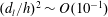 $(d_{l}/h)^{2}\sim O(10^{-1})$
, while
$(d_{l}/h)^{2}\sim O(10^{-1})$
, while
 $\unicode[STIX]{x1D716}\sim 0.01$
. Hence, we would argue that the equilibrium condition may be appropriate for the large particles but clearly breaks down for the small ones. In addition, the continuum assumption for large particles may not be completely valid, as
$\unicode[STIX]{x1D716}\sim 0.01$
. Hence, we would argue that the equilibrium condition may be appropriate for the large particles but clearly breaks down for the small ones. In addition, the continuum assumption for large particles may not be completely valid, as
 $d_{l}/h\sim 0.21$
. Despite these limitations, let us presently carry on with the equilibrium assumption in the manner of Murisic et al. (Reference Murisic, Ho, Hu, Latterman, Koch, Lin, Mata and Bertozzi2011, Reference Murisic, Pausader, Peschka and Bertozzi2013); we will later address the discrepancies of the model assumptions.
$d_{l}/h\sim 0.21$
. Despite these limitations, let us presently carry on with the equilibrium assumption in the manner of Murisic et al. (Reference Murisic, Ho, Hu, Latterman, Koch, Lin, Mata and Bertozzi2011, Reference Murisic, Pausader, Peschka and Bertozzi2013); we will later address the discrepancies of the model assumptions.
Once the left-hand side of (3.9) vanishes under the equilibrium condition, we integrate the right-hand side with respect to
 $z$
and apply the symmetry boundary condition (i.e.
$z$
and apply the symmetry boundary condition (i.e.
 $\dot{\unicode[STIX]{x1D6FE}}|_{z=0}=0$
) to obtain the following equation:
$\dot{\unicode[STIX]{x1D6FE}}|_{z=0}=0$
) to obtain the following equation:
 $$\begin{eqnarray}\frac{\unicode[STIX]{x2202}}{\unicode[STIX]{x2202}z}\left(\hat{\unicode[STIX]{x1D702}}_{n}\dot{\unicode[STIX]{x1D6FE}}\frac{\unicode[STIX]{x1D719}_{i}}{\unicode[STIX]{x1D719}}\right)=0,\end{eqnarray}$$
where the leading-order shear rate corresponds to
 $\dot{\unicode[STIX]{x1D6FE}}=\unicode[STIX]{x2202}u_{r}/\unicode[STIX]{x2202}z$
in the lubrication limit. Physically, equation (3.10) suggests that, under shear-induced migration, both particle components rearrange themselves in such a way that the particulate normal stress is constant in the
$\dot{\unicode[STIX]{x1D6FE}}=\unicode[STIX]{x2202}u_{r}/\unicode[STIX]{x2202}z$
in the lubrication limit. Physically, equation (3.10) suggests that, under shear-induced migration, both particle components rearrange themselves in such a way that the particulate normal stress is constant in the
 $z$
-direction. Similarly, under the same lubrication and equilibrium assumptions, the reduced momentum equations for the suspension are given by
$z$
-direction. Similarly, under the same lubrication and equilibrium assumptions, the reduced momentum equations for the suspension are given by
 $$\begin{eqnarray}\frac{\unicode[STIX]{x2202}P}{\unicode[STIX]{x2202}r}=\frac{\unicode[STIX]{x2202}}{\unicode[STIX]{x2202}z}(\hat{\unicode[STIX]{x1D702}}_{s}\dot{\unicode[STIX]{x1D6FE}}),\quad \frac{\unicode[STIX]{x2202}P}{\unicode[STIX]{x2202}z}=0.\end{eqnarray}$$
Integrating both sides of the
 $r$
-momentum equation with respect to
$r$
-momentum equation with respect to
 $z$
yields
$z$
yields
 $$\begin{eqnarray}\frac{\text{d}P}{\text{d}r}z=\hat{\unicode[STIX]{x1D702}}_{s}\dot{\unicode[STIX]{x1D6FE}},\end{eqnarray}$$
once the symmetry condition at the centreline (i.e.
 $\dot{\unicode[STIX]{x1D6FE}}|_{z=0}=0$
) has been applied. Finally, we arrive at the following ordinary differential equation for each particle species by combining (3.10) and (3.12):
$\dot{\unicode[STIX]{x1D6FE}}|_{z=0}=0$
) has been applied. Finally, we arrive at the following ordinary differential equation for each particle species by combining (3.10) and (3.12):
 $$\begin{eqnarray}\frac{\hat{\unicode[STIX]{x1D702}}_{n}}{\hat{\unicode[STIX]{x1D702}}_{s}}\frac{\unicode[STIX]{x1D719}_{i}}{\unicode[STIX]{x1D719}}z=\hat{\unicode[STIX]{x1D702}}_{n}\dot{\unicode[STIX]{x1D6FE}}\frac{\unicode[STIX]{x1D719}_{i}}{\unicode[STIX]{x1D719}}\left(\frac{\text{d}P}{\text{d}r}\right)^{-1}=\text{const.},\end{eqnarray}$$
which can be solved numerically subject to the fixed injection rate and input particle concentrations (3.6).
The system of equations described by (3.13) and (3.6) is highly coupled, given that
 $\unicode[STIX]{x1D719}=\unicode[STIX]{x1D719}_{s}+\unicode[STIX]{x1D719}_{l}$
. Interestingly, Lyon & Leal (Reference Lyon and Leal1998b
) experimentally showed that the small-particle concentration remains uniform across the gap and successfully incorporated the uniform
$\unicode[STIX]{x1D719}=\unicode[STIX]{x1D719}_{s}+\unicode[STIX]{x1D719}_{l}$
. Interestingly, Lyon & Leal (Reference Lyon and Leal1998b
) experimentally showed that the small-particle concentration remains uniform across the gap and successfully incorporated the uniform
 $\unicode[STIX]{x1D719}_{s}$
assumption into their mathematical model. Following their work, we will presently assume that small particles remain uniformly dispersed (i.e.
$\unicode[STIX]{x1D719}_{s}$
assumption into their mathematical model. Following their work, we will presently assume that small particles remain uniformly dispersed (i.e.
 $\unicode[STIX]{x1D719}_{s}=\unicode[STIX]{x1D719}_{s0}$
) and only impact the effective viscosity of the background suspending fluid. Our experimental measurement of the depth-averaged particle concentrations in figure 3 also supports the hypothesis that small particles remain uniform throughout the expanding suspension. In addition to decoupling the equations, this assumption allows us to work around the breakdown of the equilibrium condition for small particles (i.e.
$\unicode[STIX]{x1D719}_{s}=\unicode[STIX]{x1D719}_{s0}$
) and only impact the effective viscosity of the background suspending fluid. Our experimental measurement of the depth-averaged particle concentrations in figure 3 also supports the hypothesis that small particles remain uniform throughout the expanding suspension. In addition to decoupling the equations, this assumption allows us to work around the breakdown of the equilibrium condition for small particles (i.e.
 $\unicode[STIX]{x1D716}\ll (d_{i}/h)^{2}\ll 1$
). The failure of small particles to meet the equilibrium condition is thus circumvented by assuming the uniform distribution of small particles in the bidisperse suspension.
$\unicode[STIX]{x1D716}\ll (d_{i}/h)^{2}\ll 1$
). The failure of small particles to meet the equilibrium condition is thus circumvented by assuming the uniform distribution of small particles in the bidisperse suspension.

Figure 7. (a) The distribution of particles at
 $\unicode[STIX]{x1D719}_{0}=20\,\%$
with
$\unicode[STIX]{x1D719}_{0}=20\,\%$
with
 $\unicode[STIX]{x1D719}_{l0}$
increasing from 1 % to 5 %. Shear-induced migration is evident with concentration increases from the near-wall region to the centreline for all cases. (b) The corresponding normalised velocity profiles are presented. The classic bluntness of the velocity profile near the centreline is observed. The inset shows the zoomed-in view of the blunted region, indicating that the increase in
$\unicode[STIX]{x1D719}_{l0}$
increasing from 1 % to 5 %. Shear-induced migration is evident with concentration increases from the near-wall region to the centreline for all cases. (b) The corresponding normalised velocity profiles are presented. The classic bluntness of the velocity profile near the centreline is observed. The inset shows the zoomed-in view of the blunted region, indicating that the increase in
 $\unicode[STIX]{x1D719}_{l0}$
leads to more blunted velocity profile.
$\unicode[STIX]{x1D719}_{l0}$
leads to more blunted velocity profile.
The results of our simplified equilibrium model are shown in figure 7. For
 $\unicode[STIX]{x1D719}_{0}=20\,\%$
and
$\unicode[STIX]{x1D719}_{0}=20\,\%$
and
 $\unicode[STIX]{x1D719}_{l0}$
ranging from 1 % to 5 %, the total particle concentration
$\unicode[STIX]{x1D719}_{l0}$
ranging from 1 % to 5 %, the total particle concentration
 $\unicode[STIX]{x1D719}(z)$
and corresponding axial velocity profiles are plotted along the
$\unicode[STIX]{x1D719}(z)$
and corresponding axial velocity profiles are plotted along the
 $z$
-axis. As expected, all three
$z$
-axis. As expected, all three
 $\unicode[STIX]{x1D719}(z)$
plots in figure 7(a) show a monotonic increase from the wall (
$\unicode[STIX]{x1D719}(z)$
plots in figure 7(a) show a monotonic increase from the wall (
 $z=0.5$
) towards the centre (
$z=0.5$
) towards the centre (
 $z=0$
) due to shear-induced migration; this increase is notably greater for higher values of
$z=0$
) due to shear-induced migration; this increase is notably greater for higher values of
 $\unicode[STIX]{x1D719}_{l0}$
. Here,
$\unicode[STIX]{x1D719}_{l0}$
. Here,
 $\unicode[STIX]{x1D719}^{\prime }(z)$
appears discontinuous at
$\unicode[STIX]{x1D719}^{\prime }(z)$
appears discontinuous at
 $z=0$
, where the prime denotes the derivative with respect to
$z=0$
, where the prime denotes the derivative with respect to
 $z$
. This discontinuity in
$z$
. This discontinuity in
 $\unicode[STIX]{x1D719}^{\prime }(z)$
is the byproduct of the suspension balance model that caps
$\unicode[STIX]{x1D719}^{\prime }(z)$
is the byproduct of the suspension balance model that caps
 $\unicode[STIX]{x1D719}$
off at
$\unicode[STIX]{x1D719}$
off at
 $\unicode[STIX]{x1D719}_{m}$
as
$\unicode[STIX]{x1D719}_{m}$
as
 $\unicode[STIX]{x1D719}$
diverges with the vanishing local shear rate. Owing to the presence of particles, the velocity profiles are no longer parabolic but exhibit a blunted tip at
$\unicode[STIX]{x1D719}$
diverges with the vanishing local shear rate. Owing to the presence of particles, the velocity profiles are no longer parabolic but exhibit a blunted tip at
 $z=0$
, as shown by the plot of the normalised velocity in figure 7(b). The inset includes the zoomed-in plot of the velocity tip that becomes more blunted with an increase in
$z=0$
, as shown by the plot of the normalised velocity in figure 7(b). The inset includes the zoomed-in plot of the velocity tip that becomes more blunted with an increase in
 $\unicode[STIX]{x1D719}_{l0}$
.
$\unicode[STIX]{x1D719}_{l0}$
.
3.3 Comparisons to experiments
Since our model is only applicable to the quasi-steady flow far upstream, it cannot quantitatively describe the fingering behaviour at the interface for varying
 $\unicode[STIX]{x1D719}_{0}$
and
$\unicode[STIX]{x1D719}_{0}$
and
 $\unicode[STIX]{x1D719}_{l0}$
. However, the model should be able to capture the particle accretion dynamics towards the interface, which originates from shear-induced migration of particles upstream. Based on that, we will also consider the connection between the total amount of accumulated particles and the enhanced fingering upon the addition of large particles.
$\unicode[STIX]{x1D719}_{l0}$
. However, the model should be able to capture the particle accretion dynamics towards the interface, which originates from shear-induced migration of particles upstream. Based on that, we will also consider the connection between the total amount of accumulated particles and the enhanced fingering upon the addition of large particles.

Figure 8. (a) The depth-averaged concentration profiles acquired from experimental measurements collapse onto a single curve when normalised by the radius of the corresponding fitted circle
 $R$
. We thus argue that the upstream region corresponds to the relatively flat portion of the collapsed curve of
$R$
. We thus argue that the upstream region corresponds to the relatively flat portion of the collapsed curve of
 $\bar{\unicode[STIX]{x1D719}}$
, whose boundary is further defined as
$\bar{\unicode[STIX]{x1D719}}$
, whose boundary is further defined as
 $R_{i}$
. (b,c) Plots comparing the experimental measurements of
$R_{i}$
. (b,c) Plots comparing the experimental measurements of
 $\bar{\unicode[STIX]{x1D719}}_{l}$
and
$\bar{\unicode[STIX]{x1D719}}_{l}$
and
 $\bar{\unicode[STIX]{x1D719}}$
with the theoretical prediction show reasonable agreement.
$\bar{\unicode[STIX]{x1D719}}$
with the theoretical prediction show reasonable agreement.
Let us first test the validity of our reduced model against the measurable quantities in the experiments. For instance, figure 3 consists of the depth-averaged concentration profiles that are extracted from the experiments at time
 $t=20~\text{s}$
. Presently, we are unable to measure
$t=20~\text{s}$
. Presently, we are unable to measure
 $\unicode[STIX]{x1D719}(z)$
experimentally, due to the lack of visualisation tools. Replotting
$\unicode[STIX]{x1D719}(z)$
experimentally, due to the lack of visualisation tools. Replotting
 $\bar{\unicode[STIX]{x1D719}}$
at different times in figure 8(a) illustrates that the curves collapse when
$\bar{\unicode[STIX]{x1D719}}$
at different times in figure 8(a) illustrates that the curves collapse when
 $r$
is normalised by the location of the interface
$r$
is normalised by the location of the interface
 $R(t)$
at the given time. We hereby define the upstream region as the portion of the collapsed curve that remains relatively flat, or
$R(t)$
at the given time. We hereby define the upstream region as the portion of the collapsed curve that remains relatively flat, or
 $0<r<R_{i}(t)$
, where
$0<r<R_{i}(t)$
, where
 $R_{i}(t)/R(t)$
appears time-independent. Then, we extract the corresponding value of
$R_{i}(t)/R(t)$
appears time-independent. Then, we extract the corresponding value of
 $\bar{\unicode[STIX]{x1D719}}$
as the upstream depth-averaged particle concentration (i.e.
$\bar{\unicode[STIX]{x1D719}}$
as the upstream depth-averaged particle concentration (i.e.
 $\bar{\unicode[STIX]{x1D719}}^{exp}$
) for both the bulk suspension and large-particle component, respectively.
$\bar{\unicode[STIX]{x1D719}}^{exp}$
) for both the bulk suspension and large-particle component, respectively.
Figure 8(b,c) shows the plots of
 $\bar{\unicode[STIX]{x1D719}}^{exp}$
versus
$\bar{\unicode[STIX]{x1D719}}^{exp}$
versus
 $\bar{\unicode[STIX]{x1D719}}^{sbm}$
, the upstream depth-averaged concentrations from the simplified model, for all values of
$\bar{\unicode[STIX]{x1D719}}^{sbm}$
, the upstream depth-averaged concentrations from the simplified model, for all values of
 $\unicode[STIX]{x1D719}_{0}$
and
$\unicode[STIX]{x1D719}_{0}$
and
 $\unicode[STIX]{x1D719}_{l0}$
considered. For both total and large-particle concentrations upstream, the agreement between experiments and theory is reasonable, shown by their close collapse onto a line with slope of 1. However, given the breakdown of the continuum assumption and the discontinuity at
$\unicode[STIX]{x1D719}_{l0}$
considered. For both total and large-particle concentrations upstream, the agreement between experiments and theory is reasonable, shown by their close collapse onto a line with slope of 1. However, given the breakdown of the continuum assumption and the discontinuity at
 $z=0$
(see figure 7
a), the model is not expected to fully resolve the details of concentration profiles in
$z=0$
(see figure 7
a), the model is not expected to fully resolve the details of concentration profiles in
 $z$
. Despite these limitations, the agreement between theory and experiments in
$z$
. Despite these limitations, the agreement between theory and experiments in
 $\bar{\unicode[STIX]{x1D719}}$
demonstrates the usefulness of our reduced equilibrium model.
$\bar{\unicode[STIX]{x1D719}}$
demonstrates the usefulness of our reduced equilibrium model.
With the upstream theoretical model verified against experimental data, we now address one of the key observations of the bidisperse experiments – the preferential accumulation of large particles on the interface. As the amount and rate of particles injected into the cell are fixed, the accumulation of particles on the interface must be met by the depletion of particles from the upstream regime, or
 $\bar{\unicode[STIX]{x1D719}}<\unicode[STIX]{x1D719}_{0}$
for
$\bar{\unicode[STIX]{x1D719}}<\unicode[STIX]{x1D719}_{0}$
for
 $0<r<R_{i}(t)$
. In particular, the value of upstream
$0<r<R_{i}(t)$
. In particular, the value of upstream
 $\bar{\unicode[STIX]{x1D719}}_{l}$
relative to
$\bar{\unicode[STIX]{x1D719}}_{l}$
relative to
 $\unicode[STIX]{x1D719}_{l0}$
directly informs the depletion of large particles from the upstream and, thereby, their accumulation near the interface. Figure 9(a) shows the plot of
$\unicode[STIX]{x1D719}_{l0}$
directly informs the depletion of large particles from the upstream and, thereby, their accumulation near the interface. Figure 9(a) shows the plot of
 $\bar{\unicode[STIX]{x1D719}}_{l}$
versus
$\bar{\unicode[STIX]{x1D719}}_{l}$
versus
 $\unicode[STIX]{x1D719}_{l0}$
for
$\unicode[STIX]{x1D719}_{l0}$
for
 $\unicode[STIX]{x1D719}_{0}=20\,\%$
both from experiments (triangle) and from the suspension balance model (solid line). A dashed line of slope 1 is included to visually showcase the deviation of
$\unicode[STIX]{x1D719}_{0}=20\,\%$
both from experiments (triangle) and from the suspension balance model (solid line). A dashed line of slope 1 is included to visually showcase the deviation of
 $\bar{\unicode[STIX]{x1D719}}_{l}$
from
$\bar{\unicode[STIX]{x1D719}}_{l}$
from
 $\unicode[STIX]{x1D719}_{l0}$
, which clearly grows with
$\unicode[STIX]{x1D719}_{l0}$
, which clearly grows with
 $\unicode[STIX]{x1D719}_{l0}$
. This indicates that an increase in
$\unicode[STIX]{x1D719}_{l0}$
. This indicates that an increase in
 $\unicode[STIX]{x1D719}_{l0}$
directly increases the accumulation of large particles on the interface. Also, the same trend is evident experimentally for all values of
$\unicode[STIX]{x1D719}_{l0}$
directly increases the accumulation of large particles on the interface. Also, the same trend is evident experimentally for all values of
 $\unicode[STIX]{x1D719}_{0}$
, as shown in the inset of figure 9(a). On the other hand, figure 9(b) shows that
$\unicode[STIX]{x1D719}_{0}$
, as shown in the inset of figure 9(a). On the other hand, figure 9(b) shows that
 $\bar{\unicode[STIX]{x1D719}}_{l}$
is mostly independent of
$\bar{\unicode[STIX]{x1D719}}_{l}$
is mostly independent of
 $\unicode[STIX]{x1D719}_{0}$
for
$\unicode[STIX]{x1D719}_{0}$
for
 $\unicode[STIX]{x1D719}_{l0}=3\,\%$
and 5 %, respectively, for both experiments (symbols) and theory (solid line).
$\unicode[STIX]{x1D719}_{l0}=3\,\%$
and 5 %, respectively, for both experiments (symbols) and theory (solid line).

Figure 9. (a) Plots of
 $\bar{\unicode[STIX]{x1D719}}_{l}$
from both experimental measurements and theoretical prediction with respect to
$\bar{\unicode[STIX]{x1D719}}_{l}$
from both experimental measurements and theoretical prediction with respect to
 $\unicode[STIX]{x1D719}_{l0}$
at
$\unicode[STIX]{x1D719}_{l0}$
at
 $\unicode[STIX]{x1D719}_{0}=20\,\%$
. The observation that
$\unicode[STIX]{x1D719}_{0}=20\,\%$
. The observation that
 $\bar{\unicode[STIX]{x1D719}}_{l}$
falls below the auxiliary curve of slope 1 clearly indicates the occurrence of preferential accumulation of large particles near the interface. The inset shows all experimental measurements of
$\bar{\unicode[STIX]{x1D719}}_{l}$
falls below the auxiliary curve of slope 1 clearly indicates the occurrence of preferential accumulation of large particles near the interface. The inset shows all experimental measurements of
 $\bar{\unicode[STIX]{x1D719}}_{l}$
against
$\bar{\unicode[STIX]{x1D719}}_{l}$
against
 $\unicode[STIX]{x1D719}_{l0}$
, suggesting the trend is true for all experiments. (b) Plot of
$\unicode[STIX]{x1D719}_{l0}$
, suggesting the trend is true for all experiments. (b) Plot of
 $\bar{\unicode[STIX]{x1D719}}_{l}$
against
$\bar{\unicode[STIX]{x1D719}}_{l}$
against
 $\unicode[STIX]{x1D719}_{0}$
for
$\unicode[STIX]{x1D719}_{0}$
for
 $\unicode[STIX]{x1D719}_{l0}=3\,\%$
and 5 %. All data points fall below the auxiliary lines of their corresponding
$\unicode[STIX]{x1D719}_{l0}=3\,\%$
and 5 %. All data points fall below the auxiliary lines of their corresponding
 $\unicode[STIX]{x1D719}_{l0}$
, again confirming our observation of the preferential accumulation of large particles at the interface. Here,
$\unicode[STIX]{x1D719}_{l0}$
, again confirming our observation of the preferential accumulation of large particles at the interface. Here,
 $\bar{\unicode[STIX]{x1D719}}_{l}$
appears to be independent of
$\bar{\unicode[STIX]{x1D719}}_{l}$
appears to be independent of
 $\unicode[STIX]{x1D719}_{0}$
.
$\unicode[STIX]{x1D719}_{0}$
.
As illustrated in figure 9, our reduced model successfully captures the trend in
 $\bar{\unicode[STIX]{x1D719}}_{l}$
with
$\bar{\unicode[STIX]{x1D719}}_{l}$
with
 $\unicode[STIX]{x1D719}_{0}$
and
$\unicode[STIX]{x1D719}_{0}$
and
 $\unicode[STIX]{x1D719}_{l0}$
and can help rationalise the preferential accumulation of large particles on the interface. For instance, the model assumes that small particles remain uniformly distributed in the suspension, while the large particles migrate to the channel centre under shear-induced diffusion. Therefore, any particle accretion on the interface, or depletion from upstream, can only directly come from
$\unicode[STIX]{x1D719}_{l0}$
and can help rationalise the preferential accumulation of large particles on the interface. For instance, the model assumes that small particles remain uniformly distributed in the suspension, while the large particles migrate to the channel centre under shear-induced diffusion. Therefore, any particle accretion on the interface, or depletion from upstream, can only directly come from
 $\unicode[STIX]{x1D719}_{l0}$
. An increase in
$\unicode[STIX]{x1D719}_{l0}$
. An increase in
 $\unicode[STIX]{x1D719}_{l0}-\bar{\unicode[STIX]{x1D719}}_{l}$
with
$\unicode[STIX]{x1D719}_{l0}-\bar{\unicode[STIX]{x1D719}}_{l}$
with
 $\unicode[STIX]{x1D719}_{l0}$
naturally follows from this model assumption. In addition, our model predicts that, for given
$\unicode[STIX]{x1D719}_{l0}$
naturally follows from this model assumption. In addition, our model predicts that, for given
 $\unicode[STIX]{x1D719}_{l0}$
, increasing
$\unicode[STIX]{x1D719}_{l0}$
, increasing
 $\unicode[STIX]{x1D719}_{0}$
(or
$\unicode[STIX]{x1D719}_{0}$
(or
 $\unicode[STIX]{x1D719}_{s0}$
) only acts to enhance the background viscosity. As the shear-induced migration of large particles should be independent of the background viscosity, this explains why
$\unicode[STIX]{x1D719}_{s0}$
) only acts to enhance the background viscosity. As the shear-induced migration of large particles should be independent of the background viscosity, this explains why
 $\bar{\unicode[STIX]{x1D719}}_{l}$
does not depend on
$\bar{\unicode[STIX]{x1D719}}_{l}$
does not depend on
 $\unicode[STIX]{x1D719}_{0}$
. Overall, as previously hypothesised, the suppression of shear-induced migration of small particles and their uniform distribution are central to the notable accretion of large particles near the interface.
$\unicode[STIX]{x1D719}_{0}$
. Overall, as previously hypothesised, the suppression of shear-induced migration of small particles and their uniform distribution are central to the notable accretion of large particles near the interface.
Finally, based on mass conservation, the total particle volume that collects near the interface can be approximated by the difference between the total particle volume at time
 $t$
,
$t$
,
 $\unicode[STIX]{x1D719}_{0}\unicode[STIX]{x03C0}R(t)^{2}h$
, and that inside the upstream regime,
$\unicode[STIX]{x1D719}_{0}\unicode[STIX]{x03C0}R(t)^{2}h$
, and that inside the upstream regime,
 $\bar{\unicode[STIX]{x1D719}}\unicode[STIX]{x03C0}R_{i}(t)^{2}h$
. Normalising by
$\bar{\unicode[STIX]{x1D719}}\unicode[STIX]{x03C0}R_{i}(t)^{2}h$
. Normalising by
 $\unicode[STIX]{x03C0}R(t)^{2}h$
yields the following expression for the dimensionless amount of particles that have accumulated near the interface:
$\unicode[STIX]{x03C0}R(t)^{2}h$
yields the following expression for the dimensionless amount of particles that have accumulated near the interface:
 $$\begin{eqnarray}V^{p}\equiv \unicode[STIX]{x1D719}_{0}-\bar{\unicode[STIX]{x1D719}}\left(\frac{R_{i}}{R}\right)^{2},\end{eqnarray}$$
which is independent of time; it is straightforward to compute the value of
 $V^{p}$
from the experiments for all
$V^{p}$
from the experiments for all
 $\unicode[STIX]{x1D719}_{0}$
and
$\unicode[STIX]{x1D719}_{0}$
and
 $\unicode[STIX]{x1D719}_{l0}$
. Interestingly, the
$\unicode[STIX]{x1D719}_{l0}$
. Interestingly, the
 $V^{p}$
dependence on
$V^{p}$
dependence on
 $\unicode[STIX]{x1D719}_{l0}$
comes most directly from
$\unicode[STIX]{x1D719}_{l0}$
comes most directly from
 $R_{i}/R$
. Figure 10(a) shows that
$R_{i}/R$
. Figure 10(a) shows that
 $R_{i}/R$
monotonically decreases with
$R_{i}/R$
monotonically decreases with
 $\unicode[STIX]{x1D719}_{l0}$
, independent of
$\unicode[STIX]{x1D719}_{l0}$
, independent of
 $\unicode[STIX]{x1D719}_{0}$
. Qualitatively, this implies that the addition of large particles expedites the particle accumulation (or shortens
$\unicode[STIX]{x1D719}_{0}$
. Qualitatively, this implies that the addition of large particles expedites the particle accumulation (or shortens
 $R_{i}$
). Similarly, the inclusion of large particles was shown to expedite the time of fingering onset in § 2.3.3. While we conjecture that both expedited accumulation and fingering may be related to the time scale of particle migration, the quantitative analysis remains outside the scope of the current paper.
$R_{i}$
). Similarly, the inclusion of large particles was shown to expedite the time of fingering onset in § 2.3.3. While we conjecture that both expedited accumulation and fingering may be related to the time scale of particle migration, the quantitative analysis remains outside the scope of the current paper.

Figure 10. (a) The ratio of
 $R_{i}/R$
is plotted against
$R_{i}/R$
is plotted against
 $\unicode[STIX]{x1D719}_{l0}$
for all experiments available. The measurements of corresponding monodisperse experiments are also included here for comparison. The ratio appears to decrease monotonically with
$\unicode[STIX]{x1D719}_{l0}$
for all experiments available. The measurements of corresponding monodisperse experiments are also included here for comparison. The ratio appears to decrease monotonically with
 $\unicode[STIX]{x1D719}_{l0}$
but is independent of
$\unicode[STIX]{x1D719}_{l0}$
but is independent of
 $\unicode[STIX]{x1D719}_{0}$
as depicted by the inset. (b) Plot of
$\unicode[STIX]{x1D719}_{0}$
as depicted by the inset. (b) Plot of
 $V^{p}$
with respect to
$V^{p}$
with respect to
 $\unicode[STIX]{x1D719}_{0}$
, where each colour represents a different value of
$\unicode[STIX]{x1D719}_{0}$
, where each colour represents a different value of
 $\unicode[STIX]{x1D719}_{l0}$
. The region above the critical value
$\unicode[STIX]{x1D719}_{l0}$
. The region above the critical value
 $0.45$
is shaded in grey and almost all data points therein correspond to the ‘fingering’ regime.
$0.45$
is shaded in grey and almost all data points therein correspond to the ‘fingering’ regime.
Plotting
 $V^{p}$
from data in terms of
$V^{p}$
from data in terms of
 $\unicode[STIX]{x1D719}_{0}$
for varying
$\unicode[STIX]{x1D719}_{0}$
for varying
 $\unicode[STIX]{x1D719}_{l0}$
reveals another surprising feature (see figure 10
b). The values of
$\unicode[STIX]{x1D719}_{l0}$
reveals another surprising feature (see figure 10
b). The values of
 $\unicode[STIX]{x1D719}_{0}$
and
$\unicode[STIX]{x1D719}_{0}$
and
 $\unicode[STIX]{x1D719}_{l0}$
at which fingering initiates (see the phase diagram in figure 5) happen to fall on approximately a constant value of
$\unicode[STIX]{x1D719}_{l0}$
at which fingering initiates (see the phase diagram in figure 5) happen to fall on approximately a constant value of
 $V^{p}$
, i.e.
$V^{p}$
, i.e.
 $V_{c}^{p}\approx 0.45$
. Alternatively, the values of
$V_{c}^{p}\approx 0.45$
. Alternatively, the values of
 $\unicode[STIX]{x1D719}_{0}$
and
$\unicode[STIX]{x1D719}_{0}$
and
 $\unicode[STIX]{x1D719}_{l0}$
for which
$\unicode[STIX]{x1D719}_{l0}$
for which
 $V^{p}\gtrsim V_{c}^{p}$
yield fingering in the current experimental time scale, while those for which
$V^{p}\gtrsim V_{c}^{p}$
yield fingering in the current experimental time scale, while those for which
 $V^{p}<V_{c}^{p}$
are in the ‘no fingering’ regime. Consistent with Xu et al. (Reference Xu, Kim and Lee2016), the existence of
$V^{p}<V_{c}^{p}$
are in the ‘no fingering’ regime. Consistent with Xu et al. (Reference Xu, Kim and Lee2016), the existence of
 $V_{c}^{p}$
itself suggests that the critical onset of fingering depends on the total amount of particles that accumulate on the interface, which will be explored in future studies.
$V_{c}^{p}$
itself suggests that the critical onset of fingering depends on the total amount of particles that accumulate on the interface, which will be explored in future studies.
4 Discussion
In this paper, we experimentally demonstrate that the previously reported particle-induced fingering for monodisperse suspensions (Tang et al.
Reference Tang, Grivas, Homentcovschi, Geer and Singler2000; Xu et al.
Reference Xu, Kim and Lee2016; Kim et al.
Reference Kim, Xu and Lee2017) can be enhanced by introducing a second species of particles with larger diameter. The experiments are performed by injecting a bidisperse suspension at a constant flow rate
 $Q$
into a Hele-Shaw cell to displace air. The mixture consists of viscous silicone oil and non-colloidal neutrally buoyant particles with two distinct diameters,
$Q$
into a Hele-Shaw cell to displace air. The mixture consists of viscous silicone oil and non-colloidal neutrally buoyant particles with two distinct diameters,
 $d_{l}$
and
$d_{l}$
and
 $d_{s}$
, where
$d_{s}$
, where
 $d_{l}/d_{s}\sim 2{-}3$
; the key experimental parameters are the initial total particle volume fraction
$d_{l}/d_{s}\sim 2{-}3$
; the key experimental parameters are the initial total particle volume fraction
 $\unicode[STIX]{x1D719}_{0}$
and initial large-particle concentration
$\unicode[STIX]{x1D719}_{0}$
and initial large-particle concentration
 $\unicode[STIX]{x1D719}_{l0}$
. As we are mainly interested in the potentially significant effects that even the small addition of large particles can have on fingering,
$\unicode[STIX]{x1D719}_{l0}$
. As we are mainly interested in the potentially significant effects that even the small addition of large particles can have on fingering,
 $\unicode[STIX]{x1D719}_{l0}$
never exceeds
$\unicode[STIX]{x1D719}_{l0}$
never exceeds
 $5\,\%$
and is always below
$5\,\%$
and is always below
 $\unicode[STIX]{x1D719}_{s0}$
by a factor of 2 or more.
$\unicode[STIX]{x1D719}_{s0}$
by a factor of 2 or more.
Two series of experiments are conducted by systematically varying
 $\unicode[STIX]{x1D719}_{0}$
at fixed
$\unicode[STIX]{x1D719}_{0}$
at fixed
 $\unicode[STIX]{x1D719}_{l0}$
, or by modulating
$\unicode[STIX]{x1D719}_{l0}$
, or by modulating
 $\unicode[STIX]{x1D719}_{l0}$
at given
$\unicode[STIX]{x1D719}_{l0}$
at given
 $\unicode[STIX]{x1D719}_{0}$
. Using image processing tools and the ANN, we then extract the depth-averaged particle concentrations inside the suspension and the deformation of the suspension–air interface. Consistent with previous results, an increase in
$\unicode[STIX]{x1D719}_{0}$
. Using image processing tools and the ANN, we then extract the depth-averaged particle concentrations inside the suspension and the deformation of the suspension–air interface. Consistent with previous results, an increase in
 $\unicode[STIX]{x1D719}_{0}$
appears to induce fingering and lead to larger interfacial deformations regardless of
$\unicode[STIX]{x1D719}_{0}$
appears to induce fingering and lead to larger interfacial deformations regardless of
 $\unicode[STIX]{x1D719}_{l0}$
. However, there are two noteworthy results that are directly due to the inclusion of larger particles. First, despite the relatively small amount present in the suspension, large (red) particles are observed to consistently enrich the expanding fluid–fluid interface, in lieu of more prevalent small (green) particles. Second, for given
$\unicode[STIX]{x1D719}_{l0}$
. However, there are two noteworthy results that are directly due to the inclusion of larger particles. First, despite the relatively small amount present in the suspension, large (red) particles are observed to consistently enrich the expanding fluid–fluid interface, in lieu of more prevalent small (green) particles. Second, for given
 $\unicode[STIX]{x1D719}_{0}$
, increasing
$\unicode[STIX]{x1D719}_{0}$
, increasing
 $\unicode[STIX]{x1D719}_{l0}$
expedites the onset of fingering and, hence, shifts the transition between ‘fingering’ and ‘no fingering’ regimes.
$\unicode[STIX]{x1D719}_{l0}$
expedites the onset of fingering and, hence, shifts the transition between ‘fingering’ and ‘no fingering’ regimes.
The key to particle-induced fingering is the accumulation of particles on the interface, which generates the destabilising viscosity gradient for miscible viscous fingering. Therefore, understanding the mechanism of particle accumulation must precede the characterisation of fingering dynamics at the interface. Accordingly, we use the reduced model based on the suspension balance approach (Nott & Brady Reference Nott and Brady1994; Norman et al.
Reference Norman, Oguntade and Bonnecaze2008) to rationalise the particle accumulation of bidisperse suspensions due to shear-induced migration (Graham et al.
Reference Graham, Altobelli, Fukushima, Mondy and Stephen1991; Husband et al.
Reference Husband, Mondy, Ganani and Graham1994; Chow et al.
Reference Chow, Hamlin and Ylitalo1995; Lyon & Leal Reference Lyon and Leal1998b
). The model is used to describe the quasi-fully developed flow far upstream of the interface, where equilibrium assumptions are appropriate (Murisic et al.
Reference Murisic, Pausader, Peschka and Bertozzi2013). By assuming a uniform distribution of small particles, as evident in both our data and those of Lyon & Leal (Reference Lyon and Leal1998b
), the particle concentration and velocity profiles are numerically calculated as a function of
 $z$
. We also compute the depth-averaged concentrations of large particles in satisfactory agreement with the experimental data. The model results suggest that the suppression of shear-induced migration of small particles upstream drives the preferential accumulation of large particles at the meniscus and enhanced fingering.
$z$
. We also compute the depth-averaged concentrations of large particles in satisfactory agreement with the experimental data. The model results suggest that the suppression of shear-induced migration of small particles upstream drives the preferential accumulation of large particles at the meniscus and enhanced fingering.
This combined experimental and theoretical study builds on the previous study of particle-induced viscous fingering of monodisperse suspensions and is the first of its kind to demonstrate the role of polydispersity on fingering. Future work includes understanding the existence of the critical particle volume
 $V_{c}^{p}$
that is connected to fingering, as well as deriving a theoretical model for the onset radius of accumulation,
$V_{c}^{p}$
that is connected to fingering, as well as deriving a theoretical model for the onset radius of accumulation,
 $R_{i}/R$
, as a function of
$R_{i}/R$
, as a function of
 $\unicode[STIX]{x1D719}_{l0}$
. The present work could also be strengthened by widening the experimental parameter space, for instance, by modulating flow rates, including more than two particle types, or even changing the channel geometry. Finally, the key point to take away from the current study is that any small changes to the particle mixture that changes shear-induced migration can make a huge difference in fingering phenomena. Therefore, another exciting direction of future research lies in finding other seemingly ‘small’ ways of dramatically changing the particle-induced viscous fingering, such as the inclusion of non-spherical particles or particles of varying rigidity that alter shear-induced migration.
$\unicode[STIX]{x1D719}_{l0}$
. The present work could also be strengthened by widening the experimental parameter space, for instance, by modulating flow rates, including more than two particle types, or even changing the channel geometry. Finally, the key point to take away from the current study is that any small changes to the particle mixture that changes shear-induced migration can make a huge difference in fingering phenomena. Therefore, another exciting direction of future research lies in finding other seemingly ‘small’ ways of dramatically changing the particle-induced viscous fingering, such as the inclusion of non-spherical particles or particles of varying rigidity that alter shear-induced migration.
Appendix A. Pseudo-code for artificial neural network
In addition to the symbols introduced in § 2.2, we further define
 $\unicode[STIX]{x1D6FF}$
as the error vector, which is the difference between the classification vector and the output of the network in each iteration,
$\unicode[STIX]{x1D6FF}$
as the error vector, which is the difference between the classification vector and the output of the network in each iteration,
 $\unicode[STIX]{x1D71F}$
and
$\unicode[STIX]{x1D71F}$
and
 $\unicode[STIX]{x1D63F}$
are matrices used to store the coefficients in the process of back-propagation, and
$\unicode[STIX]{x1D63F}$
are matrices used to store the coefficients in the process of back-propagation, and
 $\unicode[STIX]{x1D709}$
represents a constant chosen empirically. The pseudo-code is given as follows:
$\unicode[STIX]{x1D709}$
represents a constant chosen empirically. The pseudo-code is given as follows:
(1) Get the training set
 $(x^{(1)},y^{(1)}),\ldots ,(x^{(m)},y^{(m)})$
(2) Set
$\unicode[STIX]{x1D6E5}_{ij}^{(l)}=0$
for all
$l,i,j$
(3) For
$i=1$
to
$m$
(i) Set
$a^{(1)}=x^{(i)}$
(ii) Perform forward propagation to compute
$a^{(l)}$
for
$l=2,3,\ldots ,L$
:
$a^{(l)}=g(W^{(l-1)}a^{(l-1)})$
(iii) Using
$y^{(i)}$
, compute
$\unicode[STIX]{x1D6FF}^{(L)}=a^{(L)}-y^{(i)}$
(iv) Compute
$\unicode[STIX]{x1D6FF}^{(L-1)}$
,
$\unicode[STIX]{x1D6FF}^{(L-2)},\ldots ,\unicode[STIX]{x1D6FF}^{(2)}$
(v)
$\unicode[STIX]{x1D6E5}_{ij}^{(l)}:=\unicode[STIX]{x1D6E5}_{ij}^{(l)}+a_{j}^{(l)}\unicode[STIX]{x1D6FF}_{i}^{(l+1)}$
(4)
$D_{ij}^{(l)}:=(1/m)\unicode[STIX]{x1D6E5}_{ij}^{(l)}+\unicode[STIX]{x1D709}W_{ij}^{(l)}$
if
$j\neq 0$
(5)
$D_{ij}^{(l)}:=(1/m)\unicode[STIX]{x1D6E5}_{ij}^{(l)}$
if
$j=0$


By the end of the algorithm, we have
 $(\unicode[STIX]{x2202}/\unicode[STIX]{x2202}W_{ij}^{(l)})J(\unicode[STIX]{x1D652})=D_{ij}^{(l)}$
, which contains the desired coefficients of the network.
$(\unicode[STIX]{x2202}/\unicode[STIX]{x2202}W_{ij}^{(l)})J(\unicode[STIX]{x1D652})=D_{ij}^{(l)}$
, which contains the desired coefficients of the network.

Figure 11. Plots of the depth-averaged concentration profiles (
 $\bar{\unicode[STIX]{x1D719}}$
(black),
$\bar{\unicode[STIX]{x1D719}}$
(black),
 $\bar{\unicode[STIX]{x1D719}}_{s}$
(green) and
$\bar{\unicode[STIX]{x1D719}}_{s}$
(green) and
 $\bar{\unicode[STIX]{x1D719}}_{l}$
(red)) as functions of radial position
$\bar{\unicode[STIX]{x1D719}}_{l}$
(red)) as functions of radial position
 $r$
for stationary bidisperse mixtures that are placed on a glass plate. All five samples have
$r$
for stationary bidisperse mixtures that are placed on a glass plate. All five samples have
 $\unicode[STIX]{x1D719}_{0}=20\,\%$
, while
$\unicode[STIX]{x1D719}_{0}=20\,\%$
, while
 $\unicode[STIX]{x1D719}_{l0}$
is varied from 1 % to 5 % by an increment of 1 %.
$\unicode[STIX]{x1D719}_{l0}$
is varied from 1 % to 5 % by an increment of 1 %.

Figure 12. Plots of the depth-averaged concentration profiles (
 $\bar{\unicode[STIX]{x1D719}}$
(black),
$\bar{\unicode[STIX]{x1D719}}$
(black),
 $\bar{\unicode[STIX]{x1D719}}_{s}$
(green) and
$\bar{\unicode[STIX]{x1D719}}_{s}$
(green) and
 $\bar{\unicode[STIX]{x1D719}}_{l}$
(red)) over
$\bar{\unicode[STIX]{x1D719}}_{l}$
(red)) over
 $r$
at early times. The top-left plot in each panel corresponds to the earliest time, and time then evolves clockwise.
$r$
at early times. The top-left plot in each panel corresponds to the earliest time, and time then evolves clockwise.
Appendix B. Calibration results for artificial neural network
For calibration purposes, the ANN method has been applied to a series of bidisperse samples with known concentrations, namely
 $\unicode[STIX]{x1D719}_{l0}=1\,\%{-}5\,\%$
, while
$\unicode[STIX]{x1D719}_{l0}=1\,\%{-}5\,\%$
, while
 $\unicode[STIX]{x1D719}_{0}$
is fixed at 20 %. The samples are prepared by carefully measuring out each component (i.e. large (red) and small (green) particles) and mixing them thoroughly in oil, before they are placed onto a plate and imaged from directly above. We then compute the depth-averaged particle concentrations using the ANN method and plot them against the radial position
$\unicode[STIX]{x1D719}_{0}$
is fixed at 20 %. The samples are prepared by carefully measuring out each component (i.e. large (red) and small (green) particles) and mixing them thoroughly in oil, before they are placed onto a plate and imaged from directly above. We then compute the depth-averaged particle concentrations using the ANN method and plot them against the radial position
 $r$
in figure 11. The results exhibit the average deviation of
$r$
in figure 11. The results exhibit the average deviation of
 $\unicode[STIX]{x1D6E5}=0.75\,\%$
, 2.87 % and 3.34 % for
$\unicode[STIX]{x1D6E5}=0.75\,\%$
, 2.87 % and 3.34 % for
 $\unicode[STIX]{x1D719}_{0}$
,
$\unicode[STIX]{x1D719}_{0}$
,
 $\unicode[STIX]{x1D719}_{s0}$
and
$\unicode[STIX]{x1D719}_{s0}$
and
 $\unicode[STIX]{x1D719}_{l0}$
, respectively, where
$\unicode[STIX]{x1D719}_{l0}$
, respectively, where
 $\unicode[STIX]{x1D6E5}=100\,\%\,|\bar{\unicode[STIX]{x1D719}}^{ANN}-\unicode[STIX]{x1D719}_{0}|/\unicode[STIX]{x1D719}_{0}$
. Overall, the calibration results demonstrate that the ANN technique effectively produces physically meaningful values of depth-averaged particle concentrations in the current set-up.
$\unicode[STIX]{x1D6E5}=100\,\%\,|\bar{\unicode[STIX]{x1D719}}^{ANN}-\unicode[STIX]{x1D719}_{0}|/\unicode[STIX]{x1D719}_{0}$
. Overall, the calibration results demonstrate that the ANN technique effectively produces physically meaningful values of depth-averaged particle concentrations in the current set-up.
Appendix C. Particle concentrations at early times
Here, we include the plots of the depth-averaged particle concentrations, i.e.
 $\bar{\unicode[STIX]{x1D719}}$
(black),
$\bar{\unicode[STIX]{x1D719}}$
(black),
 $\bar{\unicode[STIX]{x1D719}}_{s}$
(green) and
$\bar{\unicode[STIX]{x1D719}}_{s}$
(green) and
 $\bar{\unicode[STIX]{x1D719}}_{l}$
(red), at early times (around
$\bar{\unicode[STIX]{x1D719}}_{l}$
(red), at early times (around
 $r=2~\text{cm}$
) for three concentration combinations. Each panel in figure 12 contains four plots that show progression in time (starting with the top-left plot and going clockwise). A slight increase in
$r=2~\text{cm}$
) for three concentration combinations. Each panel in figure 12 contains four plots that show progression in time (starting with the top-left plot and going clockwise). A slight increase in
 $\bar{\unicode[STIX]{x1D719}}$
in the top-left subplot indicates that particles might have enriched the meniscus inside the injection tube, prior to entering the Hele-Shaw cell.
$\bar{\unicode[STIX]{x1D719}}$
in the top-left subplot indicates that particles might have enriched the meniscus inside the injection tube, prior to entering the Hele-Shaw cell.


