


1. Introduction
Electrohydrodynamics has long been a topic of fascinating research interest owing to a wide variety of far-reaching industrial implications encompassing ink-jet printing (Basaran Reference Basaran2002), electrospraying (Jaworek & Krupa Reference Jaworek and Krupa1999; Castellanos Reference Castellanos2014; Karyappa, Deshmukh & Thaokar Reference Karyappa, Deshmukh and Thaokar2014; Choi & Saveliev Reference Choi and Saveliev2017; Gañán-Calvo et al. Reference Gañán-Calvo, López-Herrera, Herrada, Ramos and Montanero2018), oil–water separation (Eow, Ghadiri & Sharif Reference Eow, Ghadiri and Sharif2007), emulsification (Karyappa, Naik & Thaokar Reference Karyappa, Naik and Thaokar2016) and so on. It all started with the benchmark finding of Taylor (Reference Taylor1966), who applied a quasi-static electric field to a neutrally buoyant and leaky-dielectric liquid droplet under the conditions of weak deformation and negligible charge convection (CC). Taylor postulated a relation between the hydrodynamic and electrical property ratios that can predict whether the drop will become prolate or oblate when placed in an electrically conducive environment. This work of Taylor (Reference Taylor1966) triggered many researchers (Ward & Homsy Reference Ward and Homsy2006; Lac & Homsy Reference Lac and Homsy2007; Zhang, Zahn & Lin Reference Zhang, Zahn and Lin2013) to explore and address some of the neglected but yet effective facets of the study.
On this note, it is important to mention literatures that are not restricted to the assumptions of Taylor (Reference Taylor1966), and instead observed the effects of an unsteady framework (Esmaeeli & Sharifi Reference Esmaeeli and Sharifi2011) and the orientation of the applied electric field (Mandal, Bandopadhyay & Chakraborty Reference Mandal, Bandopadhyay and Chakraborty2016a; Poddar et al. Reference Poddar, Mandal, Bandopadhyay and Chakraborty2019) on the electrohydrodynamic phenomenon; addressed the electrohydrodynamics of a droplet under an imposed background flow (Dey et al. Reference Dey, Ghosh, Chakraborty and Dasgupta2015); considered the complicated influence of surface CC through a nonlinear coupling (Das & Saintillan Reference Das and Saintillan2016; Poddar et al. Reference Poddar, Mandal, Bandopadhyay and Chakraborty2019) and dictated the two-way coupled influence between interfacial deformation and electrohydrodynamic characteristics of the droplet (Ha & Yang Reference Ha and Yang2000; Xu & Homsy Reference Xu and Homsy2006; Vlahovska Reference Vlahovska2011; Yariv & Almog Reference Yariv and Almog2016). In addition to surface CC and interfacial deformation, the inclusion of gravity as a body force on the droplet would result in a coupled effect due to the imposition of an external electric field – a phenomenon that can non-trivially dictate the electrohydrodynamic sedimentation of drops. Indeed, such a mechanism is of immense importance (Bandopadhyay et al. Reference Bandopadhyay, Mandal, Kishore and Chakraborty2016; Poddar et al. Reference Poddar, Mandal, Bandopadhyay and Chakraborty2018) because of its applicability in processes such as drug transportation and enzyme crystallization (Zheng, Tice & Ismagilov Reference Zheng, Tice and Ismagilov2004; Pethig Reference Pethig2013).
It is important to note that the above cited literatures are limited to studies on single droplet electrohydrodynamics. An advanced version of the same would include the analysis of a ‘compound drop’ (a core drop bounded by a shell drop) when it is affected by an electric field. Such works on compound drops are essential as they mimic the physical attributes associated with applications involving lipid bilayer formation (Palaniappan & Daripa Reference Palaniappan and Daripa2000), recovery of oil (Stone & Leal Reference Stone and Leal1990), phase separation (Draxler & Marr Reference Draxler and Marr1986) and drug transportation (Nakano Reference Nakano2000; Fabiilli et al. Reference Fabiilli, Lee, Kripfgans, Carson and Fowlkes2010). At the initial stage, investigations on compound drops were centred around studies like creeping flow mediated dynamics of a compound drop under the influence of buoyancy by Rushton & Davies (Reference Rushton and Davies1983) and inertia by Brunn & Roden (Reference Brunn and Roden1985); translational stability of compound drops by Sadhal & Oguz (Reference Sadhal and Oguz1985); influence of extensional flows on the compound drop dynamics by Stone & Leal (Reference Stone and Leal1990) and many others of the kind extensively reviewed in Johnson & Sadhal (Reference Johnson and Sadhal1985) – literatures that neglected the effect of an externally imposed electric field. However, an electric field, after it has been widely applied and proved effective in modulating the sedimentation of single drop (Xu & Homsy Reference Xu and Homsy2006; Bandopadhyay et al. Reference Bandopadhyay, Mandal, Kishore and Chakraborty2016; Poddar et al. Reference Poddar, Mandal, Bandopadhyay and Chakraborty2018), was applied to compound drops to understand the electrohydrodynamics involved.
The earliest literature investigating the stability of an eccentric compound drop due to the effect of buoyancy and an electric field was presented by Gouz & Sadhal (Reference Gouz and Sadhal1989). They coupled the leaky-dielectric model to the creeping flow equations and semi-analytically solved the same for spherical drops in a bipolar coordinate system. Tsukada et al. (Reference Tsukada, Mayama, Sato and Hozawa1997) conducted experiments and computations to gain insight into the concomitant effects of an electric field and convection on the degree of deformation of a compound drop. Finally, the authors showed that the electric intensity and the core to shell drop volume ratio could correlate the deformation of the drop and the strength of flow. For leaky-dielectric fluids, Behjatian & Esmaeeli (Reference Behjatian and Esmaeeli2013) analytically showed that the flow pattern inside and outside a compound drop subjected to a weak electric field is dictated by the number of vortices in the shell. Soni, Juvekar & Naik (Reference Soni, Juvekar and Naik2013) observed shape transition (oblate to prolate or vice versa) for a double emulsion under a uniformly oriented electric field. Thereafter, the electrohydrodynamics of a compound drop was studied under an alternating current environment in some literature (Soni, Dixit & Juvekar Reference Soni, Dixit and Juvekar2017; Soni, Thaokar & Juvekar Reference Soni, Thaokar and Juvekar2018).
Recently, Santra, Mandal & Chakraborty (Reference Santra, Mandal and Chakraborty2019) considered the pressure driven flow of a compound droplet in a transversely applied electric field. Their study addressed the droplet pinch-off dynamics because of a displacement of the core from the concentric point. The authors also examined the transient electrohydrodynamic phenomenon of a confined compound drop through numerical and analytical techniques in one of their works (Santra, Das & Chakraborty Reference Santra, Das and Chakraborty2020). However, surface CC was not accounted for in any of the aforementioned literature. Moreover, the involved electrohydrodynamics can also be tuned by the deformation of the compound drop (Bandopadhyay et al. Reference Bandopadhyay, Mandal, Kishore and Chakraborty2016). Hence, it has been established for simple drops that shape deformation and CC act as two key electrohydrodynamic determinants (Mandal et al. Reference Mandal, Sinha, Bandopadhyay and Chakraborty2018). In the latest work from our group (Boruah et al. Reference Boruah, Randive, Pati and Sahu2022), one such study was taken up where the problem of a compound drop moving under the action of background plane Poiseuille flow and acted upon by an applied electric field was investigated. In this case, a neutrally buoyant compound drop configuration is considered to highlight the sole effect of background flow. However, if the compound drop is allowed to sediment under the action of buoyancy in an electrically conducive environment, then the physics of the problem would be governed by a balance between the associated forces and the buoyancy force. In such a situation, the electrohydrodynamics of the compound drop would be critically influenced by the density of the involved phases, and this would be an interesting problem to investigate.
Motivated by the same, the buoyancy driven settling of a compound drop in an electrically conducive environment is analytically formalized for both the concentric and eccentric configurations. A detailed study is carried out for an eccentric compound drop subjected to applied electric field and is solved semi-analytically in a bispherical coordinate system in this article; however, a similar study for a concentric compound drop configuration can be performed using the method outlined in Boruah et al. (Reference Boruah, Randive, Pati and Sahu2022). For both the cases, the sedimentation velocity of the two drops (shell and core) is determined, and the same is applied to capture the influence of concomitant physical, hydrodynamic and electric properties on compound droplet sedimentation. Thereafter, the critical limit of eccentricity and time within which similar results are furnished by concentric and eccentric configurations is determined.
2. Problem formulation
2.1. Physical description
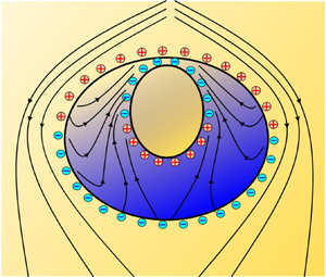
A physical scenario of an eccentric compound drop with Ro as the outer radius and Ri as the inner radius of the undeformed configuration that sediments with a priori unknown uniform shell drop velocity ( $\boldsymbol{\mathsf{U}}_{2}$) and core drop velocity (
 $\boldsymbol{\mathsf{U}}_{3}$) in a surrounding unbounded phase due to the co-presence of gravity and an electric field
  $({\boldsymbol{\mathsf{E}}_\infty })$ uniformly applied, as shown in figure 1(a), is considered. A bispherical coordinate system
  $(\xi ,\eta ,\varphi )$ is considered which is attached to the centroid of the drop. In the schematic,
  ${\xi _1} = {\cosh ^{ - 1}}((1 + {e^2} - {K^2})/2e)$ represents the shell drop interface and
  ${\xi _2} = {\cosh ^{ - 1}}((1 - {e^2} - {K^2})/2eK)$ denotes the core drop interface, where e indicates the eccentricity and K indicates radius ratio, i.e. the ratio of the radius of the core drop to the radius of the shell drop. Note that the numbers 1, 2 and 3 are used to designate the suspending phase, the shell drop phase and the core drop phase, respectively. Density is denoted by
  ${\rho _i}$, viscosity by
  ${\mu _i}$, electrical permittivity by
  ${\varepsilon _i}$ and electrical conductivity by
  ${\sigma _i}$ for the ith fluid. On the other hand, subscript ‘ij’ is used to refer to the interface separating the ith and jth fluids and, accordingly, we denote the interfacial tension by
  ${\gamma _{ij}}$.

Figure 1. Representative schematic of an eccentric compound drop configuration sedimenting in the presence of both gravity and a uniform imposed electric field.
2.2. Assumptions
The mathematical model is simplified using the following assumptions:
(i) The flows in all the three phases of fluids are considered to be incompressible. The core drop is not miscible in the shell and similarly the shell drop is immiscible in the suspending medium.
(ii) The fluids are considered to be leaky dielectric and Newtonian in nature.
(iii) Each of the fluid phases flows at a hydrodynamic Reynolds number
 $(Re = {\rho _1}{U_c}{R_o}/{\mu _1})$ much less than unity such that the Stokes equations are applicable. Here, ${U_c}$ is the characteristic velocity defined as ${U_c} = R_o^2g{\rho _1}/{\mu _1}$, where g is defined as the acceleration due to gravity.
(iv) Under the creeping flow limit, the magnitude of the capillary number
$(Ca = {\mu _1}{U_c}/{\gamma _{12}})$ is considered to be low enough such that the spherical shape of the drops is maintained.(v) At all times, quasi-steady flow is maintained such that the fluid motion is dictated by the instantaneous droplet position.
(vi) The stability of the compound drop system is maintained.


2.3. Experimental justification for the assumptions
The present theory has been set up on the assumptions outlined in the previous section and requires a suitable parametric space to connect itself to real world problems. To relate to practical experiments such as those in Xu & Homsy (Reference Xu and Homsy2006), we consider the suspending medium and the core drop to be castor oil  $({\rho _{1,3}} = 961\;\textrm{kg}\;{\textrm{m}^{ - 3}},\;{\mu _{1,3}} = 1.4\;\textrm{Pa}\;\textrm{s},\;{\epsilon _{1,3}} = 4.45{\epsilon _0},\;{\sigma _{1,3}} = 5 \times {10^{ - 10}}\;\textrm{S}\;{\textrm{m}^{ - 1}})$, where
  ${\epsilon _0}$ as the permittivity of vacuum, while phenylmethylsiloxane-dimethylsiloxane
  $({\rho _2} = 1000\;\textrm{kg}\;{\textrm{m}^{ - 3}},\;{\mu _2} = 0.5\;\textrm{Pa}\;\textrm{s},\;{\epsilon _2} = 2.8{\epsilon _0},\;{\sigma _2} = {10^{ - 12}}\;\textrm{S}\;{\textrm{m}^{ - 1}})$ is the shell drop fluid. The interfacial tension is taken to be
  $\gamma = 5 \times {10^{ - 3}}\;\textrm{N}\;{\textrm{m}^{ - 1}}$. To adhere to the assumptions considered herein, we consider Ro = 200 μm and
  ${E_\infty } = {E_{ref}} = 2 \times {10^5}\;\textrm{V}\;{\textrm{m}^{ - 1}}$.
With the aforementioned parametric set-up, the assumptions can be justified as follows: firstly, these fluids are Newtonian and immiscible, thus supporting assumptions (i) and (ii) in the previous section. They are also leaky dielectric (assumption (ii)) as the time scale for relaxation of charges,  ${\varepsilon _1}/{\sigma _1}$ is less than the time scale for convection of charges,
  ${R_o}/{U_c}$. Stokes flow (assumption (iii)) is also valid as
  $Re\sim {10^{ - 4}}$. The capillary number
  $(Ca\sim 0.1)$ is low enough, thus validating assumption (iv). Although the compound drop would temporally evolve, the associated fluid motion would depend on the instantaneous location of the droplets, allowing us to consider quasi-steady flow (assumption (v)), as previously done in the literature (Pak, Feng & Stone Reference Pak, Feng and Stone2014). Moreover, the generation of a stable compound drop (assumption (vi)) is practically feasible by actuating bi-phase flow in narrow capillaries (Utada et al. Reference Utada, Lorenceau, Link, Kaplan, Stone and Weitz2005; Kim et al. Reference Kim, Kim, Cho and Weitz2011).
2.4. Non-dimensional scheme
The non-dimensional scheme employs Ro as the length scale;  ${U_c} = R_o^2g{\rho _1}/{\mu _1}$ as the velocity scale; Eref as the electric intensity scale;
  ${\mu _1}{U_c}/{R_o}( = \boldsymbol{\tau }_{ref}^H)$ as the hydrodynamic stress scale; and
  ${\varepsilon _1}E_{ref}^2( = \boldsymbol{\tau }_{ref}^E)$ as the electric stress scale. Similarly, we define different property ratios such as the viscosity ratio by
  ${\lambda _{1i}} = {\mu _i}/{\mu _1}$, conductivity ratio by
  ${R_{1i}} = {\sigma _i}/{\sigma _1}$, permittivity ratio by
  ${S_{1i}} = {\varepsilon _i}/{\varepsilon _1}$ and radius ratio by
  $K = {R_i}/{R_o}$.
2.5. Governing equations and boundary conditions
We start with the governing equation for electric field intensity i.e.
 \begin{equation}\boldsymbol{\nabla } \times {\boldsymbol{E}_i} = 0,\end{equation}
which can be reformulated as (Sadhal Reference Sadhal1983)
 \begin{equation}{\boldsymbol{E}_i} ={-} \boldsymbol{\nabla }{\psi _i} = \boldsymbol{\nabla } \times \left( {\frac{{{\omega_i}}}{\rho }{{\hat{\boldsymbol{i}}}_\varphi }} \right).\end{equation}
Substituting (2.2) into (2.1) yields
 \begin{equation}\boldsymbol{\nabla } \times \boldsymbol{\nabla } \times \left( {\frac{{{\omega_i}}}{\rho }} \right){\hat{\boldsymbol{i}}_\varphi } = 0,\end{equation}
where  $\boldsymbol{\nabla } = \widehat {{\boldsymbol{\iota}_{\boldsymbol{\eta }}}}{h_1}\partial /\partial \eta + \widehat {{\boldsymbol{\iota}_{\boldsymbol{\xi }}}}{h_2}\partial /\partial \xi + \widehat {{\boldsymbol{\iota}_{\boldsymbol{\varphi }}}}{h_3}\partial /\partial \varphi $,
  ${h_1} = {h_2} = (\cosh \xi - \zeta )/c$ and
  ${h_3} = (\cosh \xi - \zeta )/(c\sqrt {1 - {\zeta ^2}} )$, with
  $\zeta = \cos \eta $ and
  $c = K\sinh {\xi _1}$.
Further simplification of (2.3) yields  ${\varepsilon ^2}{\omega _i} = 0$, with the expression for
  ${\varepsilon ^2}$ as (Stimson & Jeffery Reference Stimson and Jeffery1926)
 \begin{equation}{\varepsilon ^2} \equiv \frac{{(\cosh \xi - \zeta )}}{{{c^2}}}\left[ {\frac{\partial }{{\partial \xi }}\left\{ {(\cosh \xi - \zeta )\frac{\partial }{{\partial \xi }}} \right\} + (1 - {\zeta^2})\frac{\partial }{{\partial \zeta }}\left\{ {(\cosh \xi - \zeta )\frac{\partial }{{\partial \zeta }}} \right\}} \right].\end{equation}
As given in Wacholder & Weihs (Reference Wacholder and Weihs1972),  $\omega $ has the following solution:
 \begin{equation}\omega = {(\cosh \xi - \zeta )^{ - 1/2}}\sum\limits_{n = 0}^\infty {\left[ {{d_n}\cosh \left( {n + \frac{1}{2}} \right)\xi + {e_n}\sinh \left( {n + \frac{1}{2}} \right)\xi } \right]C_{n + 1}^{ - 1/2}(\zeta )} ,\end{equation}
where, the Gegenbauer polynomial  $C_{n + 1}^{ - 1/2}$ is of degree −1/2 and order (n + 1). For different involved regions,
  ${\omega _i}$ has the following forms that satisfy the far field condition at the leading order (
 ${\omega _1} \to {\rho ^2}/2$, as
  $\xi ,\eta \to 0$) and the boundedness condition (
 $|{\omega _3}|< \infty$, as
  $\xi \to \infty$) in bispherical coordinates (Morton, Subramanian & Balasubramaniam Reference Morton, Subramanian and Balasubramaniam1990)
 \begin{gather}{\omega _1} = \frac{{{\rho ^2}}}{2} + {(\cosh \xi - \zeta )^{ - 1/2}}\sum\limits_{n = 0}^\infty {\left[ {{d_n}\sinh \left( {n + \frac{1}{2}} \right)\xi } \right]C_{n + 1}^{ - 1/2}(\zeta )} ,\end{gather}
 \begin{gather}{\omega _2} = {(\cosh \xi - \zeta )^{ - 1/2}}\sum\limits_{n = 0}^\infty {[{f_n}\,{\textrm{e}^{(n + 1/2)(\xi - {\xi _2})}} + {g_n}\,{\textrm{e}^{ - (n + 1/2)(\xi - {\xi _2})}}]C_{n + 1}^{ - 1/2}(\zeta )} ,\end{gather}
 \begin{gather}{\omega _3} = {(\cosh \xi - \zeta )^{ - 1/2}}\sum\limits_{n = 0}^\infty {[{h_n}\,{\textrm{e}^{ {\mp} (n + 1/2)(\xi - {\xi _2})}}]C_{n + 1}^{ - 1/2}(\zeta )} .\end{gather}
Utilizing the well-known relations  $\rho = c\sqrt {1 - {\zeta ^2}} /(\cosh \xi - \zeta ),\;z = c\sinh \xi /(\cosh \xi - \zeta ),\;\varphi \textrm{ = }\varphi$, the remaining boundary conditions will take the following form Gouz & Sadhal (Reference Gouz and Sadhal1989):
 \begin{gather}{\left. {\frac{{\partial {\omega_i}}}{{\partial \xi }}} \right|_{\xi = {\xi _i}}} = {\left. {\frac{{\partial {\omega_j}}}{{\partial \xi }}} \right|_{\xi = {\xi _i}}},\end{gather}
 \begin{gather}{R_{1i}}{\omega _i}{|_{\xi = {\xi _i}}} = {R_{1j}}{\omega _j}{|_{\xi = {\xi _i}}}.\end{gather}
 Towards solving the flow problem, the governing equation  ${\varepsilon ^4}{S_i} = 0$, with S being the Stokes streamfunction is used (Happel & Brenner Reference Happel and Brenner2012) which has a general solution of the following form for ith fluid (Stimson & Jeffery Reference Stimson and Jeffery1926):
 \begin{equation}{S_i} = {(\cosh \xi - \zeta )^{ - 3/2}}\sum\limits_{n = 0}^\infty {\varXi _n^{(i)}(\xi )C_{n + 1}^{ - 1/2}(\zeta )} .\end{equation}
As given in Mandal, Ghosh & Chakraborty (Reference Mandal, Ghosh and Chakraborty2016b),  $\Xi _n^{(i )}$ will assume the following forms:
 \begin{gather}\varXi _n^{(1)} = {D_n}\,{\textrm{e}^{(n - 1/2)\xi }} + {E_n}\,{\textrm{e}^{(n + 3/2)\xi }} + {\tilde{f}_n}\,{\textrm{e}^{ {\mp} (n - 1/2)\xi }} + {\tilde{g}_n}\,{\textrm{e}^{ {\mp} (n + 3/2)\xi }},\end{gather}
 \begin{gather}\varXi _n^{(2)} = {H_n}\,{\textrm{e}^{(n - 1/2)\xi }} + {I_n}\,{\textrm{e}^{(n + 3/2)\xi }} + {J_n}\,{\textrm{e}^{ {\mp} (n - 1/2)\xi }} + {K_n}\,{\textrm{e}^{ {\mp} (n + 3/2)\xi }},\end{gather}
 \begin{gather}\varXi _n^{(3)} = {L_n}\,{\textrm{e}^{ {\mp} (n - 1/2)\xi }} + {M_n}\,{\textrm{e}^{ {\mp} (n + 3/2)\xi }}.\end{gather}
Using these relations, the leading-order far field condition can be recast as (Mandal et al. Reference Mandal, Ghosh and Chakraborty2016b)
 \begin{equation}{S_1} = {(\cosh \xi - \zeta )^{ - 3/2}}\sum\limits_{n = 0}^\infty {({{\tilde{f}}_n}\,{\textrm{e}^{ {\mp} (n - 1/2)\xi }} + {{\tilde{g}}_n}\,{\textrm{e}^{ {\mp} (n + 3/2)\xi }})C_{n + 1}^{ - 1/2}\textrm{(}\zeta \textrm{)}\;\textrm{as}\;\xi \to 0} .\end{equation}
Here, the constants  ${\tilde{f}_n}\;\textrm{and}\;{\tilde{g}_n}$ can be expressed as (Mandal et al. Reference Mandal, Ghosh and Chakraborty2016b)
 \begin{equation}{\tilde{f}_n} = \frac{{n(n + 1){c^2}}}{{\sqrt 2 (2n - 1)}}{U_2}\quad \textrm{and}\quad {\tilde{g}_n} ={-} \frac{{n(n + 1){c^2}}}{{\sqrt 2 (2n + 3)}}{U_2}.\end{equation}
The leading-order hydrodynamic boundary conditions are as follows (Gouz & Sadhal Reference Gouz and Sadhal1989):
 \begin{gather}u_\xi ^{(i)} = u_\xi ^{(j)} = {\delta _{i2}}({\boldsymbol{\mathsf{U}}_3} - {\boldsymbol{\mathsf{U}}_2}) \boldsymbol{\cdot} {\hat{\boldsymbol{i}}_\xi },\end{gather}
 \begin{gather}u_\eta ^{(i)} = u_\eta ^{(j)},\end{gather}
 \begin{gather}{\lambda _i}\tau _{\xi \eta }^{(i)} - {\lambda _j}\tau _{\xi \eta }^{(j)} = \frac{{E_\eta ^{(i)}}}{{4{\rm \pi}}}({S_{1j}}E_\xi ^{(j)} - {S_{1i}}E_\xi ^{(i)}).\end{gather}
The electrostatic and hydrodynamic equations are first linearized to suitable forms given in Appendix A and Appendix B. Thereafter, they are solved semi-analytically using the procedure outlined in Boruah et al. (Reference Boruah, Randive, Pati and Sahu2022) and Jadhav & Ghosh (Reference Jadhav and Ghosh2021a), which is not repeated herein for the sake of brevity. This results in unknown coefficients which are then utilized along with force balance conditions to determine the velocities. The force balance equations are (Sadhal & Oguz Reference Sadhal and Oguz1985)
 \begin{gather}{\aleph _{21}}{U_2} + {\aleph _{31}}{U_3} + {\aleph _1} = \frac{2}{{3\sqrt 2 c}}[{K^3}{\rho _{13}} + (1 - {K^3}){\rho _{12}} - 1],\end{gather}
 \begin{gather}{\aleph _{22}}{U_2} + {\aleph _{32}}{U_3} + {\aleph _2} = \frac{2}{{3\sqrt 2 c}}[{K^3}({\rho _{13}} - {\rho _{12}})],\end{gather}
where  ${\aleph _{21}} = \sum\nolimits_{n = 0}^N {(\vartheta _2^{(1)} + \vartheta _2^{(2)})} ,\;{\aleph _{31}} = \sum\nolimits_{n = 0}^N {(\vartheta _3^{(1)} + \vartheta _3^{(2)})} \textrm{,}\;{\aleph _1} = \sum\nolimits_{n = 0}^N {(\vartheta _1^{(1)} + \vartheta _1^{(2)})}$ and so on.
3. Results and Discussion
First, the results for the shell and core drop velocities using the eccentric configuration and concentric configuration are compared under the small eccentricity limit (e = 0.001). The details of the solution procedure regarding sedimentation of a concentric compound drop can be found in Boruah et al. (Reference Boruah, Randive, Pati and Sahu2022). Note that the problem discussed in Boruah et al. (Reference Boruah, Randive, Pati and Sahu2022) is for a neutrally buoyant compound drop migrating under the action of plane Poiseuille flow and an electric field. However, the aforementioned problem can be simplified to the case of a compound drop sedimenting under the action of gravity and an electric field by setting the coefficients of the velocity profile accordingly and modifying the force balance condition to include the effect of density.
We start with a comparative study of the results for shell and core drop velocities using the eccentric configuration and concentric configuration under the small eccentricity limit and for two different combinations of R 12 and S 12 (i.e. R 12 < S 12 and R 12 > S 12), as shown in figure 2. As a function of radius ratio, the variation in velocity for the two drops are showcased in figures 2(a) and 2(b) for a suitable choice of parameter ratios as provided in the figure caption. The plots clearly indicate perfect matching between the results of the eccentric compound drop obtained using bispherical coordinates and the analytical results of a concentric compound drop. Moreover, we notice that the core size hinders the movement of both drops, as they slow down with the increase in K. However, the effect of K in altering the velocity is more pronounced in the core drop as compared with the shell drop. Furthermore, it is important to notice that both drops migrate in the direction of gravity when they are concentric (or eccentricity is very low), irrespective of the choice of R 12 and S 12.

Figure 2. Comparison of (a) shell drop velocity (U 2) vs radius ratio (K) and (b) core drop velocity (U 3) vs K for eccentric compound drop with e = 0.001 and concentric compound drop for R 12 < S 12 (R 12 = 1.5, S 12 = 2) and R 12 > S 12 (R 12 = 1.1, S 12 = 0.5). The other considered ratios are  ${\rho _{12}} = 1.04$,
  ${\rho _{13}} = 1$,
  ${\lambda _{12}} = 0.5$,
  ${\lambda _{13}} = 1$,
  ${R_{13}} = 1$ and
  ${S_{13}} = 1$.
We also present a comparative study of the results for shell and core drop velocities using the eccentric compound drop configuration in the small eccentricity limit (e = 0.001), and for viscosity ratio values of 0.1, 1 and 10, and those of concentric compound drop in figure 3. As a function of K, the variation in velocity for the core and shell is, respectively, showcased in figures 3(a) and 3(b) for a suitable choice of parameter ratios, as mentioned in the caption of the figure. Here also, an accurate match between the results of the eccentric compound drop obtained using bispherical coordinates and the analytical results of the concentric case is noticed for different values of  ${\lambda _{12}}$. The core and shell velocities decrease as
  ${\lambda _{12}}$ increases. It is also important to notice that the size of the core drop can either aid or hinder the movement of the shell and core drop based on
  ${\lambda _{12}}$. Indeed for
  ${\lambda _{12}} \le 1$, both the core and shell velocities decrease as K increases. On the contrary, for
  ${\lambda _{12}} > 1$, both the core and shell velocities increase with K owing to the decrease in volume of the highly viscous fluid in the shell drop.

Figure 3. Comparison of (a) shell drop velocity (U 2) vs radius ratio (K) and (b) core drop velocity (U 3) vs K for eccentric compound drop with e = 0.001 and concentric compound drop for different values of  ${\lambda _{12}}$. The other considered property ratios are
  ${\rho _{12}} = 1.04$,
  ${\rho _{13}} = 1$,
  ${\lambda _{13}} = 1$,
  ${R_{12}} = 1.5$,
  ${R_{13}} = 1$,
  ${S_{12}} = 2$ and
  ${S_{13}} = 1$.
Next, we move on towards analysing the impact of the hydrodynamic and electric parameters on the motion of an eccentric compound drop. We start with the variation of the core and shell velocities under the influence of the density ratio  $({\rho _{12}})$ for e = 0.001(concentric), 0.1, 0.3 and 0.5, as depicted in figure 4. The other relevant parameters are given in the caption of figure 4. We can notice the concomitant interplay of eccentricity and density ratio in tuning the direction and speed of both drops. The velocities of the shell and core drop for e = 0.1 deviate minimally from the results for a concentric compound drop and show minimum alteration in the migration direction with change in
  ${\rho _{12}}$. However, with the increase in eccentricity, we observe that both drops migrate along the direction of the applied electric field when
  ${\rho _{12}} < 1$, while they migrate opposite to the direction of the applied electric field when
  ${\rho _{12}} > 1$. Also, the higher the deviation of the density ratio is from 1, the higher are the magnitudes of the core and shell velocities, and the same also increase as the eccentricity increases. The reason behind such an intriguing variation in the direction and velocity of core and shell because of the confluence of the eccentricity and density ratio can be attributed to the asymmetry in the fluid accumulated above and below the core with the change in eccentricity. Additionally, the presence of dense fluid either inside or outside the shell drop also aids or hinders the asymmetricity in the charge distribution due to the supplied electric field, thus mediating the droplet direction.

Figure 4. Variation of (a) shell drop velocity (U 2) and (b) core drop velocity (U 3) with  ${\rho _{12}}$ for e = 0.1, 0.3, 0.5 and 0.001 (concentric). The other considered parameters are
  ${\rho _{13}} = 1$,
  ${\lambda _{12}} = 0.5$,
  ${\lambda _{13}} = 1$,
  ${R_{12}} = 1.5$,
  ${R_{13}} = 1$,
  ${S_{12}} = 2$ and
  ${S_{13}} = 1$.
Figure 5 demonstrates the shell and core drop velocity variations as a function of viscosity ratio  $({\lambda _{12}})$ for e = 0.001(concentric), 0.1, 0.3 and 0.5, under a suitable choice of property ratios, as mentioned in the figure caption. At lower values of
  ${\lambda _{12}}$, the velocity variation is more significant as compared with that at higher values of
  ${\lambda _{12}}$. Indeed, a finite velocity occurs when the viscosity ratio is sufficiently higher. This underscores the profound influence of the presence of a viscous fluid either inside or outside the shell drop which aids or hinders the asymmetricity in the charge distribution because of the supplied electric field, thus manipulating the velocity of the drops. Apart from the effect of the viscosity in tuning the magnitude of the velocity, the eccentricity critically mitigates the direction of drop motion. For the concentric configuration and e = 0.1, the shell and core drops are seen to migrate along the direction of the applied electric field, while they migrate opposite to that of applied electric field when the eccentricity is sufficiently large. The asymmetry in the accumulated fluid above and below the core with a change in eccentricity is the reason behind such an observation.

Figure 5. Variation of (a) shell drop velocity (U 2) and (b) core drop velocity (U 3) with  ${\lambda _{12}}$ for e = 0.1, 0.3, 0.5 and 0.001 (concentric). The other considered parameters are
  ${\rho _{12}} = 1.04$,
  ${\rho _{13}} = 1$,
  ${\lambda _{13}} = 1$,
  ${R_{12}} = 1.5$,
  ${R_{13}} = 1$,
  ${S_{12}} = 2$ and
  ${S_{13}} = 1$.
In terms of the influence of the electric parameters, firstly, we show the variation of the shell and core drop velocities in figures 6(a) and 6(b), respectively, with a change in electrical conductivity ratio  $({R_{12}})$ for e = 0.001(concentric), 0.1, 0.3 and 0.5. The remaining property ratios considered here are given in the caption of figure 6. Here also, the variations in velocity with R 12 for e = 0.1 and the concentric configuration depict close agreement. More precisely, we notice significant variation in the velocity when R 12 < 1, beyond which the variation in velocity with R 12 is insignificant. Quantitatively, the magnitudes of the core and shell velocities decrease as R 12 increases and this decrease is sharp for R 12 < 1. This happens because the asymmetricity in the charge distribution decreases with the increase in R 12. Also, it is to be noted that
  ${S_{12}} = 2$ in figure 6, and therefore, the core and shell velocities alter in sign when R 12 > 2, depending also on the value of eccentricity. Indeed, when the eccentricity is sufficiently large, both the core and shell velocities remain negative (i.e. they migrate opposite to the direction of the applied electric field) throughout, irrespective of the variation in R 12. This happens because the imbalance in fluid accumulation above and below the core drop due to the variation of eccentricity nullifies the effect of the asymmetric charge distribution when the eccentricity is very large.

Figure 6. Variation of (a) shell drop velocity (U 2) and (b) core drop velocity (U 3) with  ${R_{12}}$ for e = 0.1, 0.3, 0.5 and 0.001 (concentric). The other considered parameters are
  ${\rho _{12}} = 1.04$,
  ${\rho _{13}} = 1$,
  ${\lambda _{12}} = 0.5$,
  ${\lambda _{13}} = 1$,
  ${R_{13}} = 1$,
  ${S_{12}} = 2$ and
  ${S_{13}} = 1$.
Figure 7 demonstrates the variation of shell and core drop velocities with electrical permittivity ratio  $({S_{12}})$ for e = 0.001(concentric), 0.1, 0.3 and 0.5. The remaining property ratios considered here are given in the caption of figure 7. As is evident, with the increase in S 12, the shell and core drop velocities may either decrease or increase or alter sign depending on e. More precisely, we notice an alteration in the migration direction of both the core and shell for e = 0.1, and an increase in the velocity of the drops when the eccentricity is sufficiently higher (i.e. e = 0.5) due to the increase in S 12. Such a variation occurs because the effect of the disbalance in fluid accumulation above and below the core due to the change in e nullifies the effect of the asymmetric charge distribution when the eccentricity is very large and, hence, we observe either an increase or decrease in velocity with the increase in S 12.

Figure 7. Variation of (a) shell drop velocity (U 2) and (b) core drop velocity (U 3) with  ${S_{12}}$ for e = 0.1, 0.3, 0.5 and 0.001 (concentric). The other considered parameters are
  ${\rho _{12}} = 1.04$,
  ${\rho _{13}} = 1$,
  ${\lambda _{12}} = 0.5$,
  ${\lambda _{13}} = 1$,
  ${R_{12}} = 1.5$,
  ${R_{13}} = 1$ and
  ${S_{13}} = 1$.
The next task is to explore whether an equilibrium configuration (for any e) exists and how the same is influenced by the hydrodynamic and electrical property ratios. We do so by plotting the variation of the relative velocity between the two drops (shell and core) i.e. U 2–U 3, for different values of eccentricity and observe its variation with a change in property ratios. Figure 8(a) shows the plot of U 2–U 3 variation as a function of  ${\rho _{12}}$. At first, it is to be noted that, for
  ${\rho _{12}} < 1$, U 2–U 3 < 0, for almost all values of the eccentricity. This indicates faster movement of the core drop relative to the shell drop. However, when
  ${\rho _{12}} > 1$, U 2–U 3 > 0, for almost all values of the eccentricity. This alteration in sign indicates the presence of the critical density ratio
  $({\rho _{12}} = 1)$ for each e, for which U 2 = U 3. Also, the more the value of
  ${\rho _{12}}$ is higher or lower than the critical
  ${\rho _{12}}$, the larger is the difference in the relative velocity of the two drops. Furthermore, we observe that the difference in the relative velocity is the lowest for the concentric configuration and
  $e \le 0.1$, indicating the fact that the concentric compound drop furnishes similar results as the eccentric compound drop up to an eccentricity limit of 0.1, irrespective of the density ratio considered.

Figure 8. (a) Variation of (U 2–U 3) with  ${\rho _{12}}$ for e = 0.1, 0.3, 0.5 and 0.001 (concentric). (b) Evolution of eccentricity e(t) with time (t), subjected to e(t = 0) = 0, for
  ${\rho _{12}} = 0.1,\textrm{ }1.04\;\textrm{and}\;10$. The other considered parameters are
  ${\rho _{13}} = 1$,
  ${\lambda _{12}} = 0.5$,
  ${\lambda _{13}} = 1$,
  ${R_{12}} = 1.5$,
  ${R_{13}} = 1$,
  ${S_{12}} = 2$ and
  ${S_{13}} = 1$.
The existence of a non-zero relative velocity is indicative of the fact that the eccentricity of the compound drop evolves with time. With the progress of time, there is a linear increase in the rate of eccentricity (e) as follows:  $e(t) = ({U_{2,z}}\unicode{x2013} {U_{3,z}})t$. Hence, for the validity of the concentric assumption, two conditions need to be satisfied. The first condition is that
  $e \ll 1$ or
  $|{U_{2,z}}\unicode{x2013} {U_{3,z}}|\ll 1$. Even though the first condition is satisfied, however, the eccentricity being a function of time would increase as time progresses. Therefore,
  $t < |{U_{2,z}}/({U_{2,z}}\unicode{x2013} {U_{3,z}})|$ is the second essential condition for the validity of the concentric assumption. Indeed, our results quantitatively support the concentric compound drop assumption as shown in Appendix C.
This would continue until the core drop migrates, reaches a stable fixed point and moves with the same velocity as the shell drop thereafter. In order to ascertain the same, the following differential equation is solved numerically to determine how the eccentricity evolves with time:
 \begin{equation}\frac{{\textrm{d}e}}{{\textrm{d}t}} = [{U_3}(e(t),\Pi ) - {U_2}(e(t),\Pi )].\end{equation}
By solving (3.1), the temporal evolution of the eccentricity for different  ${\rho _{12}}$ is depicted in figure 8(b). From the figure, we observe that the closer the value of
  ${\rho _{12}}$ is to the critical
  ${\rho _{12}}$, the smaller is the stable fixed eccentricity point and the larger is the time taken to attain the same. However, irrespective of the value of
  ${\rho _{12}}$, the eccentricity in general remains lower than 0.1 within a non-dimensional time limit of the order of 102. This indicates that the concentric compound drop configuration and eccentric configuration can furnish similar results until the time limit mentioned above.
In figure 9(a), we present the variation in the relative velocity of the core and shell with a viscosity ratio  $({\lambda _{12}})$ for different eccentricities. It clearly indicates that an equilibrium configuration exists at the critical viscosity ratio limit of around 10, deviation from which manifests as the core velocity being either higher or lower than the shell velocity. In fact, the least deviation from the stable equilibrium position is observed for an eccentricity near approximately 0.3. However, it is also seen that, irrespective of the value of
  ${\lambda _{12}}$, the concentric compound drop configuration predicts a similar variation in U 2–U 3 as that for e = 0.1. Moreover, to examine the point of stability in terms of eccentricity and non-dimensional time for different
  ${\lambda _{12}}$, we plot the temporal evolution of eccentricity for different
  ${\lambda _{12}}$ in figure 9(b) by solving (3.1). From the figure, we observe that the closer the value of
  ${\lambda _{12}}$ is to the critical viscosity ratio, the smaller is the stable fixed eccentricity point and the greater is the time taken to attain the same. However, irrespective of the value of
  ${\lambda _{12}}$, the eccentricity in general remains lower than 0.1 within a non-dimensional time range of the order of 102–103.

Figure 9. (a) Variation of (U 2–U 3) with  ${\lambda _{12}}$ for e = 0.1, 0.3, 0.5 and 0.001 (concentric). (b) Evolution of eccentricity e(t) with time (t), subjected to e(t = 0) = 0, for
  ${\lambda _{12}} = 0.1,\textrm{ }1\;\textrm{and}\;10$. The other considered parameters are
  ${\rho _{12}} = 1.04$,
  ${\rho _{13}} = 1$,
  ${\lambda _{13}} = 1$,
  ${R_{12}} = 1.5,$
  ${R_{13}} = 1$,
  ${S_{12}} = 2$ and
  ${S_{13}} = 1$.
Next, we examine the implication of the electrical parameters for the relative drop velocity and for the temporal evolution of eccentricity. Figure 10(a) depicts the variation in the relative velocity of the core and shell with  ${R_{12}}$ for different eccentricities. The plot indicates maximum deviation from the stable equilibrium configuration for very small values of R 12. As R 12 increases, the tendency of the core to attain a stable configuration increases, although it is the maximum when R 12 = S 12. Moreover, the relative velocity of the drops increases with the decrease in eccentricity. We also observe that, irrespective of the value of
  ${R_{12}}$, the concentric compound drop configuration predicts a similar variation in U 2–U 3 as that for e = 0.1. Thereafter, to examine the point of stability in terms of eccentricity and non-dimensional time for different
  ${R_{12}}$, we plot the temporal evolution of eccentricity for different
  ${R_{12}}$ in figure 10(b). From the figure, we observe that the smaller is deviation of
  ${R_{12}}$ from the critical conductivity ratio, the smaller is the stable fixed eccentricity point and the larger is the time taken to attain the same. However, irrespective of the value of
  ${R_{12}}$, the eccentricity in general remains lower than 0.1 within a non-dimensional time limit of the order of 102, the condition under which the concentric and eccentric configurations furnish similar results.

Figure 10. (a) Variation of (U 2–U 3) with  ${R_{12}}$ for e = 0.1, 0.3, 0.5 and 0.001 (concentric). (b) Evolution of eccentricity e(t) with time (t), subjected to e(t = 0) = 0, for
  ${R_{12}} = 0.1,\textrm{ }1.5\;\textrm{and}\;3$. The other considered parameters are
  ${\rho _{12}} = 1.04$,
  ${\rho _{13}} = 1$,
  ${\lambda _{12}} = 0.5$,
  ${\lambda _{13}} = 1$,
  ${R_{13}} = 1$,
  ${S_{12}} = 2$ and
  ${S_{13}} = 1$.
Finally, the variation in the relative velocity of the core and shell with  ${S_{12}}$ for different eccentricities is presented in figure 11(a) for a suitable choice of property ratios, as mentioned in the figure caption. The plot indicates that
  ${U_2}\unicode{x2013} {U_3}$ is close to zero for S 12 = R 12 when e = 0.1 for the concentric configuration, indicating S 12 = R 12 as the critical permittivity limit pertaining to a stable configuration for this case. However, with the increase in eccentricity, we notice that the critical permittivity limit also changes. Thereafter, we plot the temporal evolution of the eccentricity for different
  ${S_{12}}$ in figure 11(b) to examine the point of stability in terms of eccentricity and non-dimensional time for different
  ${S_{12}}$. We observe that smaller is the deviation of
  ${S_{12}}$ from the critical permittivity ratio, the smaller is the stable fixed eccentricity point and the smaller is the time taken to attain the same. However, irrespective of the value of
  ${S_{12}}$, the eccentricity in general remains lower than 0.1 within a non-dimensional time limit of the order of 102. Under this condition, both configurations of compound drop furnish similar results.

Figure 11. (a) Variation of (U 2–U 3) with  ${S_{12}}$ for e = 0.1, 0.3, 0.5 and 0.001 (concentric). (b) Evolution of eccentricity e(t) with time (t), subjected to e(t = 0) = 0, for
  ${S_{12}} = 0.1,\textrm{ }1.5\;\textrm{and}\;3$. The other considered parameters are
  ${\rho _{12}} = 1.04$,
  ${\rho _{13}} = 1$,
  ${\lambda _{12}} = 0.5$,
  ${\lambda _{13}} = 1$,
  ${R_{12}} = 1.5$,
  ${R_{13}} = 1$ and
  ${S_{13}} = 1$.
4. Conclusions
Considering a practical situation of an eccentric compound drop sedimenting in the presence of a uniform electric field, we semi-analytically determine the sedimentation velocity of the two drops (shell and core), and the same is applied to capture the influence of concomitant physical, hydrodynamic and electric properties on compound droplet sedimentation. Thereafter, the critical limit of eccentricity and time within which similar results are furnished by the concentric and eccentric configurations is determined. The salient features of the present study for an eccentric compound drop can be summarized as follows:
(i) In the case of an eccentric compound drop, the density ratio critically controls the direction of migration of the drops when the eccentricity is high. However, the viscosity ratio tunes the magnitude of the shell and core drop velocities without affecting the direction of motion.
(ii) At lower values of the eccentricity, the core and shell alter their direction of motion when R 12 = S 12, while they always migrate opposite to the direction of the applied electric field when the eccentricity is sufficiently large, irrespective of the variation in conductivity ratio. On the other hand, with the increase in S 12, the core and shell velocities may either decrease or increase or alter sign based on the eccentricity.
(iii) In terms of the relative velocity between the core and shell, there exists a critical hydrodynamic or electrical parameter ratio above or below which the core drop might move at a velocity higher or lower than the shell drop. This critical density ratio is 1 and the critical viscosity ratio is 10. In terms of the conductivity ratio, the critical ratio is at R 12 = S 12. However, it is found that the critical permittivity limit also changes with eccentricity.
(iv) Moreover, regardless of the value of the parameter ratio, the concentric configuration can predict similar variation in the relative velocity as that obtained for e = 0.1 and hence, the concentric and eccentric compound drop configurations furnish similar results up to e < 0.1. Indeed, from the temporal evolution of the eccentricity, the stable fixed eccentricity point and the non-dimensional time required to attain the same are determined for different values of the property ratios. It is found that, based on the property ratios, the eccentricity remains lower than 0.1 up to a non-dimensional time range of the order of 102–103, within which both configurations can furnish similar solutions.
Acknowledgements
The authors would like to acknowledge U. Ghosh and S.N. Jadhav for insightful discussions regarding the numerical solution of eccentric compound drop configuration. The authors would also like to acknowledge S. Mandal for insightful discussions regarding the solution for the concentric compound drop configuration.
Declaration of interests
The authors report no conflict of interest.
Appendix A. Algebraic equations for the electric potential field
The following linear algebraic equations are obtained by converting the boundary conditions (2.7) (Jadhav & Ghosh Reference Jadhav and Ghosh2021b):
 \begin{gather} {[} -
{d_{n - 1}}{{\it R} _{4n}} + {f_{n - 1}}{{\it R} _{5n}} - {g_{n -
1}}{{\it R} _{6n}}](n + 1) + {d_n}{\varUpsilon _{1n}} -
{f_n}{\varUpsilon _{2n}} + {g_n}{\varUpsilon _{3n}}\nonumber\\ + [
- {d_{n + 1}}{{\it R} _{7n}} + {f_{n + 1}}{{\it R} _{8n}} - {g_{n +
1}}{{\it R} _{9n}}]n = 4\sqrt 2 n(n + 1){c^2}\,{\textrm{e}^{
{\mp} (n + 1/2){\xi _1}}}\sinh {\xi _1},
\end{gather}
\begin{gather} {[} -
{d_{n - 1}}{{\it R} _{4n}} + {f_{n - 1}}{{\it R} _{5n}} - {g_{n -
1}}{{\it R} _{6n}}](n + 1) + {d_n}{\varUpsilon _{1n}} -
{f_n}{\varUpsilon _{2n}} + {g_n}{\varUpsilon _{3n}}\nonumber\\ + [
- {d_{n + 1}}{{\it R} _{7n}} + {f_{n + 1}}{{\it R} _{8n}} - {g_{n +
1}}{{\it R} _{9n}}]n = 4\sqrt 2 n(n + 1){c^2}\,{\textrm{e}^{
{\mp} (n + 1/2){\xi _1}}}\sinh {\xi _1},
\end{gather}
 \begin{gather} -{[}{f_{n - 1}} - {g_{n -
1}} + {h_{n - 1}}](n + 1) + {f_n}{\varUpsilon _{4n}} -
{g_n}{\varUpsilon _{5n}} + {h_n}{\varUpsilon _{5n}} -
[{f_{n + 1}} - {g_{n + 1}} + {h_{n + 1}}]n = 0,\end{gather}
\begin{gather} -{[}{f_{n - 1}} - {g_{n -
1}} + {h_{n - 1}}](n + 1) + {f_n}{\varUpsilon _{4n}} -
{g_n}{\varUpsilon _{5n}} + {h_n}{\varUpsilon _{5n}} -
[{f_{n + 1}} - {g_{n + 1}} + {h_{n + 1}}]n = 0,\end{gather}
 \begin{gather}- {d_n}{{\it R} _{1n}} +
[{f_n}{{\it R} _{2n}} + {g_n}{{\it R} _{3n}}]{R_{12}} = 4\sqrt 2
n(n + 1){c^2}\,{\textrm{e}^{ {\mp} (n + 1/2){\xi
_1}}},\end{gather}
\begin{gather}- {d_n}{{\it R} _{1n}} +
[{f_n}{{\it R} _{2n}} + {g_n}{{\it R} _{3n}}]{R_{12}} = 4\sqrt 2
n(n + 1){c^2}\,{\textrm{e}^{ {\mp} (n + 1/2){\xi
_1}}},\end{gather}
 \begin{gather} {[}{f_n} + {g_n}]{R_{12}}
- {h_n}{R_{13}} = 0,\end{gather}
\begin{gather} {[}{f_n} + {g_n}]{R_{12}}
- {h_n}{R_{13}} = 0,\end{gather}
where,  ${{\it R} _{1n}} = \sinh (n + 1/2){\xi _1};\;{{\it R} _{2n}} = {\textrm{e}^{(n + 1/2)({\xi _1} - {\xi _2})}};\;{{\it R} _{3n}} = {\textrm{e}^{ - (n + 1/2)({\xi _1} - {\xi _2})}}$
 \begin{gather}{{\it R} _{4n}} = \cosh \left( {n - \frac{1}{2}} \right){\xi _1};\quad {{\it R} _{5n}} = {\textrm{e}^{(n - 1/2)({\xi _1} - {\xi _2})}};\quad {{\it R} _{6n}} = {\textrm{e}^{ - (n - 1/2)({\xi _1} - {\xi _2})}};\end{gather}
 \begin{gather}{{\it R} _{7n}} = \cosh \left( {n + \frac{3}{2}} \right){\xi _1};\quad {{\it R} _{8n}} = {\textrm{e}^{(n + 3/2)({\xi _1} - {\xi _2})}};\quad {{\it R} _{9n}} = {\textrm{e}^{ - (n + 3/2)({\xi _1} - {\xi _2})}};\end{gather}
 \begin{gather}{\Upsilon _{1n}} = (2n + 1)\cosh {\xi _1}\cosh \left( {n + \frac{1}{2}} \right){\xi _1} - {{\it R} _{1n}}\sinh {\xi _1};\end{gather}
 \begin{gather}{\varUpsilon _{2n}} = [(2n + 1)\cosh {\xi _1} - \sinh {\xi _1}]{{\it R} _{2n}};\quad {\varUpsilon _{3n}} = [(2n + 1)\cosh {\xi _1} + \sinh {\xi _1}]{{\it R} _{3n}};\end{gather}
 \begin{gather}{\varUpsilon _{4n}} = (2n + 1)\cosh {\xi _2} - \sinh {\xi _2};\quad {\varUpsilon _{5n}} = (2n + 1)\cosh {\xi _2} + \sinh {\xi _2}.\end{gather}
Appendix B. Algebraic equations for the hydrodynamic field
The algebraic equations for the hydrodynamic field are as follows:
 \begin{equation}{D_n}\varLambda _n^1 + {E_n}\varLambda _n^2 = {U_2}\varLambda _n^3\left( {\frac{{\Lambda_n^4}}{{(2n - 1)}} - \frac{{\Lambda_n^5}}{{(2n + 3)}}} \right),\end{equation}
 \begin{equation}{H_n}\varLambda _n^1 + {I_n}\varLambda _n^2 + {J_n}\varLambda _n^4 + {K_n}\varLambda _n^5 = 0,\end{equation}
 \begin{equation}{(}2n - 1)\{ ({D_n} \,{-}\, {H_n})\varLambda _n^1 + {J_n}\varLambda _n^4\} + (2n + 3)\{ ({E_n} \,{-}\, {I_n})\varLambda _n^2 + {K_n}\varLambda _n^5\} ={-} {U_2}\varLambda _n^3(\varLambda _n^4 - \varLambda _n^5),\end{equation}
 \begin{align} &{(2n -
1)^2}\{ ({D_n} - {\lambda _2}{H_n})\varLambda _n^1 -
{\lambda _2}{J_n}\varLambda _n^4\} + {(2n + 3)^2}\{ ({E_n}
- {\lambda _2}{I_n})\varLambda _n^2 - {\lambda
_2}{K_n}\varLambda _n^5\}\nonumber \\ &\quad= \varLambda
_n^6\left( {\dfrac{{{S_{12}}}}{{{R_{12}}}} - 1}
\right)\left[ \begin{array}{@{}l@{}} \dfrac{{(2n +
1)\Lambda_n^7}}{2}\left\{ {c\varOmega_{n,k}^1 -
{c^2}\varOmega_{n,k}^2 - \dfrac{1}{c}\Lambda_k^8\varOmega_{n,k}^3
- \dfrac{1}{{2c}}\Lambda_k^9\varOmega_{n,k}^4} \right\}\\
\quad + \Lambda_n^{10}\sinh {\xi_1}\left\{ { -
\dfrac{c}{2}\varOmega_{n,k}^5 +
\dfrac{{{c^2}}}{2}\varOmega_{n,k}^6 +
\dfrac{1}{{2c}}\Lambda_k^8\varOmega_{n,k}^7 +
\dfrac{1}{{2c}}\Lambda_k^9\varOmega_{n,k}^8} \right\}
\end{array} \right]\nonumber\\ &\qquad- {U_2}\varLambda
_n^3((2n - 1)\varLambda _n^4 - (2n + 3)\varLambda
_n^5),\end{align}
\begin{align} &{(2n -
1)^2}\{ ({D_n} - {\lambda _2}{H_n})\varLambda _n^1 -
{\lambda _2}{J_n}\varLambda _n^4\} + {(2n + 3)^2}\{ ({E_n}
- {\lambda _2}{I_n})\varLambda _n^2 - {\lambda
_2}{K_n}\varLambda _n^5\}\nonumber \\ &\quad= \varLambda
_n^6\left( {\dfrac{{{S_{12}}}}{{{R_{12}}}} - 1}
\right)\left[ \begin{array}{@{}l@{}} \dfrac{{(2n +
1)\Lambda_n^7}}{2}\left\{ {c\varOmega_{n,k}^1 -
{c^2}\varOmega_{n,k}^2 - \dfrac{1}{c}\Lambda_k^8\varOmega_{n,k}^3
- \dfrac{1}{{2c}}\Lambda_k^9\varOmega_{n,k}^4} \right\}\\
\quad + \Lambda_n^{10}\sinh {\xi_1}\left\{ { -
\dfrac{c}{2}\varOmega_{n,k}^5 +
\dfrac{{{c^2}}}{2}\varOmega_{n,k}^6 +
\dfrac{1}{{2c}}\Lambda_k^8\varOmega_{n,k}^7 +
\dfrac{1}{{2c}}\Lambda_k^9\varOmega_{n,k}^8} \right\}
\end{array} \right]\nonumber\\ &\qquad- {U_2}\varLambda
_n^3((2n - 1)\varLambda _n^4 - (2n + 3)\varLambda
_n^5),\end{align}
 \begin{equation}{H_n}\varLambda _n^1 + {I_n}\varLambda _n^2 + {J_n}\varLambda _n^4 + {K_n}\varLambda _n^5 = ({U_2} - {U_3})\varLambda _n^3\left( {\frac{{\Lambda_n^4}}{{(2n - 1)}} - \frac{{\Lambda_n^5}}{{(2n + 3)}}} \right),\end{equation}
 \begin{equation}{L_n}\varLambda _n^4 + {M_n}\varLambda _n^5 = ({U_2} + {U_3})\varLambda _n^3\left( {\frac{{\Lambda_n^4}}{{(2n - 1)}} - \frac{{\Lambda_n^5}}{{(2n + 3)}}} \right),\end{equation}
 \begin{equation}{(}2n - 1)\{ {H_n}\varLambda _n^1 + ({L_n} - {J_n})\varLambda _n^4\} + (2n + 3)\{ {I_n}\varLambda _n^2 + ({M_n} - {K_n})\varLambda _n^5\} = 0,\end{equation}
 \begin{align}&
{(2n - 1)^2}\{ {\lambda _2}{H_n}\varLambda _n^1 + ({\lambda
_2}{J_n} - {\lambda _3}{L_n})\varLambda _n^4\} + {(2n +
3)^2}\{ {\lambda _2}{I_n}\varLambda _n^1 + ({\lambda
_2}{K_n} - {\lambda _3}{M_n})\varLambda _n^4\} \nonumber\\ & \quad =
\varLambda _n^6\left(
{\dfrac{{{S_{12}}{R_{13}}}}{{{R_{12}}}} - {S_{13}}}
\right)\left[ \begin{array}{@{}l@{}} \dfrac{{(2n +
1)\Lambda_n^7}}{2}\left\{ { -
\dfrac{1}{c}\Lambda_k^8\varOmega_{n,k}^3 -
\dfrac{1}{{2c}}\Lambda_k^9\varOmega_{n,k}^4} \right\}\\ +
\Lambda_n^{10}\sinh {\xi_2}\left\{
{\dfrac{1}{{2c}}\Lambda_k^8\varOmega_{n,k}^7 +
\dfrac{1}{{2c}}\Lambda_k^9\varOmega_{n,k}^8} \right\}
\end{array} \right]\nonumber\\ & \quad \quad \textrm{ + (}{U_2} -
{U_3}\textrm{)(}{\lambda _2} - {\lambda
_3}\textrm{)}\varLambda _n^3((2n - 1)\varLambda _n^4 - (2n
+ 3)\varLambda _n^5). \end{align}
\begin{align}&
{(2n - 1)^2}\{ {\lambda _2}{H_n}\varLambda _n^1 + ({\lambda
_2}{J_n} - {\lambda _3}{L_n})\varLambda _n^4\} + {(2n +
3)^2}\{ {\lambda _2}{I_n}\varLambda _n^1 + ({\lambda
_2}{K_n} - {\lambda _3}{M_n})\varLambda _n^4\} \nonumber\\ & \quad =
\varLambda _n^6\left(
{\dfrac{{{S_{12}}{R_{13}}}}{{{R_{12}}}} - {S_{13}}}
\right)\left[ \begin{array}{@{}l@{}} \dfrac{{(2n +
1)\Lambda_n^7}}{2}\left\{ { -
\dfrac{1}{c}\Lambda_k^8\varOmega_{n,k}^3 -
\dfrac{1}{{2c}}\Lambda_k^9\varOmega_{n,k}^4} \right\}\\ +
\Lambda_n^{10}\sinh {\xi_2}\left\{
{\dfrac{1}{{2c}}\Lambda_k^8\varOmega_{n,k}^7 +
\dfrac{1}{{2c}}\Lambda_k^9\varOmega_{n,k}^8} \right\}
\end{array} \right]\nonumber\\ & \quad \quad \textrm{ + (}{U_2} -
{U_3}\textrm{)(}{\lambda _2} - {\lambda
_3}\textrm{)}\varLambda _n^3((2n - 1)\varLambda _n^4 - (2n
+ 3)\varLambda _n^5). \end{align}
The notations used in (B1) have the following expressions:
 \begin{align}&\varLambda _n^1 =
{\textrm{e}^{(n - 1/2)\xi }},\quad \varLambda _n^2 =
{\textrm{e}^{(n + 3/2)\xi }},\quad \varLambda _n^3 = n(n +
1){c^2}/\sqrt 2 ,\nonumber\\ &\varLambda _n^4 = {\textrm{e}^{ - (n
- 1/2)\xi }},\quad \varLambda _n^5 = {\textrm{e}^{ - (n +
3/2)\xi }},\end{align}
\begin{align}&\varLambda _n^1 =
{\textrm{e}^{(n - 1/2)\xi }},\quad \varLambda _n^2 =
{\textrm{e}^{(n + 3/2)\xi }},\quad \varLambda _n^3 = n(n +
1){c^2}/\sqrt 2 ,\nonumber\\ &\varLambda _n^4 = {\textrm{e}^{ - (n
- 1/2)\xi }},\quad \varLambda _n^5 = {\textrm{e}^{ - (n +
3/2)\xi }},\end{align}
 \begin{equation}\varLambda _n^6 = \frac{{n(n + 1)(2n + 1)}}{{2{\rm \pi}}},\quad \varLambda _n^7 = {f_n}\,{\textrm{e}^{(n + 1/2)(\xi - {\xi _2})}} - {g_n}\,{\textrm{e}^{ - (n + 1/2)(\xi - {\xi _2})}},\end{equation}
 \begin{equation}\varLambda _k^8 = \sum\limits_{k = 0}^N {{d_k}\sinh \left( {k + \frac{1}{2}} \right)\xi C_k^{1/2}} ,\quad \varLambda _k^9 = \sum\limits_{k = 0}^N {{d_k}\sinh \left( {k + \frac{1}{2}} \right)\xi C_{k + 1}^{ - 1/2}} ,\end{equation}
 \begin{equation}\varLambda _n^{10} = {f_n}\,{\textrm{e}^{(n + 1/2)(\xi - {\xi _2})}} + {g_n}\,{\textrm{e}^{ - (n + 1/2)(\xi - {\xi _2})}},\end{equation}
 \begin{equation}\varOmega _{n,k}^1(\xi ) = \int_{ - 1}^1 {\frac{{xC_{n + 1}^{ - 1/2}C_{k + 1}^{ - 1/2}}}{{(1 - {x^2})}}\,\textrm{d}\kern0.06em x} ,\quad \varOmega _{n,k}^2(\xi ) = \int_{ - 1}^1 {\frac{{C_{n + 1}^{ - 1/2}C_{k + 1}^{ - 1/2}}}{{(\cosh \xi - x)}}\,\textrm{d}\kern0.06em x} ,\end{equation}
 \begin{equation}\varOmega _{n,k}^3(\xi ) = \int_{ - 1}^1 {\frac{{{{(\cosh \xi - x)}^{3/2}}C_{n + 1}^{ - 1/2}C_{k + 1}^{ - 1/2}}}{{{{(1 - {x^2})}^{3/2}}}}\,\textrm{d}\kern0.06em x} ,\quad \varOmega _{n,k}^4(\xi ) = \int_{ - 1}^1 {\frac{{{{(\cosh \xi - x)}^{1/2}}C_{n + 1}^{ - 1/2}C_{k + 1}^{ - 1/2}}}{{(1 - {x^2})}}\,\textrm{d}\kern0.06em x} ,\end{equation}
 \begin{equation}\varOmega _{n,k}^5(\xi ) = \int_{ - 1}^1 {\frac{{xC_{n + 1}^{ - 1/2}C_{k + 1}^{ - 1/2}}}{{(1 - {x^2})(\cosh \xi - x)}}\,\textrm{d}\kern0.06em x} ,\quad \varOmega _{n,k}^6(\xi ) = \int_{ - 1}^1 {\frac{{C_{n + 1}^{ - 1/2}C_{k + 1}^{ - 1/2}}}{{{{(\cosh \xi - x)}^2}}}\,\textrm{d}\kern0.06em x} ,\end{equation}
 \begin{equation}\varOmega _{n,k}^7(\xi ) = \int_{ - 1}^1 {\frac{{{{(\cosh \xi - x)}^{1/2}}C_{n + 1}^{ - 1/2}C_{k + 1}^{ - 1/2}}}{{{{(1 - {x^2})}^{3/2}}}}\,\textrm{d}\kern0.06em x} ,\quad \varOmega _{n,k}^8(\xi ) = \int_{ - 1}^1 {\frac{{C_{n + 1}^{ - 1/2}C_{k + 1}^{ - 1/2}}}{{{{(\cosh \xi - x)}^{1/2}}(1 - {x^2})}}\,\textrm{d}\kern0.06em x} .\end{equation}
Equations (B1a)–(B1d) are for  $\xi = {\xi _1}$ and (B1e)–(B1h) are for
  $\xi = {\xi _2}$.
Appendix C. Condition for the validity of the concentric compound drop configuration
In order to determine the condition within which the concentric assumption is valid, we plot the eccentricity variation with time for various K in figure 12. Previously, it has been established that the concentric and eccentric theories deliver similar results when the eccentricity e < 0.1 (Mandal et al. Reference Mandal, Ghosh and Chakraborty2016b). From figure 12, we determine that the aforementioned condition is satisfied when the dimensionless time ranges from 450 to 850. Beyond this, the eccentric theory (Jadav & Ghosh Reference Jadhav and Ghosh2021a,Reference Jadhav and Ghoshb) needs to be applied.

Figure 12. Temporal variation of eccentricity for various K in case of concentric compound drop. The other considered parameters are  ${\theta _t} = {\rm \pi}/4,\;{R_{12}} = 1.5,\;{R_{13}} = 1,\;{S_{12}} = 2,\;{S_{13}} $
  $= 1,\;{\rho _{12}} = 1.04,\;{\rho _{13}} = 1,\;{\lambda _{12}} = 0.5,\;{\lambda _{13}} = 1,\;M = 1,\;Ca = 0.1$ and
  $R{e_E} = 0.1$.


