


1. Introduction
Resolvent analysis constitutes an input-output framework between forces and their responses in the frequency domain. This approach has attracted the attention of the fluid mechanics community after McKeon & Sharma (Reference McKeon and Sharma2010) used it to model a turbulent channel flow, showing that if forcing terms show no preferential direction, the flow response is dominated by the optimal response mode. In this case, Towne, Schmidt & Colonius (Reference Towne, Schmidt and Colonius2018) showed that these optimal response modes provide an approximation of coherent structures within the flow as defined by spectral proper orthogonal decomposition. Several studies applied the same ideas to other flows (Beneddine et al. Reference Beneddine, Sipp, Arnault, Dandois and Lesshafft2016; Abreu, Cavalieri & Wolf Reference Abreu, Cavalieri and Wolf2017; Schmidt et al. Reference Schmidt, Towne, Rigas, Colonius and Brès2018; Lesshafft et al. Reference Lesshafft, Semeraro, Jaunet, Cavalieri and Jordan2019; Yeh & Taira Reference Yeh and Taira2019), and to develop estimation methods (Gómez et al. Reference Gómez, Blackburn, Rudman, Sharma and McKeon2016a; Beneddine et al. Reference Beneddine, Yegavian, Sipp and Leclaire2017; Sasaki et al. Reference Sasaki, Piantanida, Cavalieri and Jordan2017; Symon Reference Symon2018; Martini et al. Reference Martini, Cavalieri, Jordan, Towne and Lesshafft2020; Towne, Lozano-Durán & Yang Reference Towne, Lozano-Durán and Yang2020).
If the flow has one non-homogeneous direction, resolvent modes and gains can be obtained by direct manipulation of the matrix that represents the discretized system (McKeon & Sharma Reference McKeon and Sharma2010). When a direct matrix decomposition is not possible, iterative methods are needed. These can typically be divided into two parts:  $(a)$ obtaining the effect of the resolvent operator acting on a vector, and
  $(b)$ algorithms that use
  $(a)$ to approximate singular values and vectors. To distinguish these, we will refer to
  $(a)$ as ‘methods’ and to
  $(b)$ as ‘algorithms’.
Different methods have been used in the literature. The effect of the resolvent operator on a vector can be obtained by solving a linear system of equations. An LU factorization has been used to solve the linear system and obtain resolvent modes iteratively (Sipp & Marquet Reference Sipp and Marquet2013; Schmidt et al. Reference Schmidt, Towne, Rigas, Colonius and Brès2018; Ribeiro, Yeh & Taira Reference Ribeiro, Yeh and Taira2020). Brynjell-Rahkola et al. (Reference Brynjell-Rahkola, Tuckerman, Schlatter and Henningson2017) solved the linear problem using a GMRES method, which was accelerated with the use of preconditioners on flows with low Reynolds numbers. Monokrousos et al. (Reference Monokrousos, Åkervik, Brandt and Henningson2010) used a matrix-free approach, using time marching of the direct and adjoint equations. On each iteration, the system was harmonically forced with the previous iteration result until the steady-state response was reached, repeating the method until convergence provides optimal force and response modes for a given frequency. Gómez, Sharma & Blackburn (Reference Gómez, Sharma and Blackburn2016b) obtained an 80 % reduction of the total integration time for this method by considering complex-valued periodic functions and using improved initial conditions. However, the approach can only recover the leading mode at each frequency.
The power iteration algorithm is popular (Monokrousos et al. Reference Monokrousos, Åkervik, Brandt and Henningson2010; Gómez et al. Reference Gómez, Sharma and Blackburn2016b), but it only provides the leading mode. Alternatively, the Arnoldi algorithm (Arnoldi Reference Arnoldi1951) is able to recover optimal and suboptimal modes (Jeun, Nichols & Jovanović Reference Jeun, Nichols and Jovanović2016; Schmidt et al. Reference Schmidt, Towne, Rigas, Colonius and Brès2018; Lesshafft et al. Reference Lesshafft, Semeraro, Jaunet, Cavalieri and Jordan2019). Another approach is the randomized singular-value decomposition, first used for resolvent analysis by Moarref et al. (Reference Moarref, Sharma, Tropp and McKeon2013) and further explored by Ribeiro et al. (Reference Ribeiro, Yeh and Taira2020), where an algebraic convergence rate with the number of random vectors used was observed.
Alternatively, reduced-order models (ROMs) have been used to approach such systems, e.g. ROMS based on the system eigenmodes (Åkervik et al. Reference Åkervik, Ehrenstein, Gallaire and Henningson2008; Alizard, Cherubini & Robinet Reference Alizard, Cherubini and Robinet2009; Schmid & Henningson Reference Schmid and Henningson2012). However, a truncated set of eigenmodes does not necessarily provide an effective basis for the system (Trefethen Reference Trefethen1997; Rodríguez, Tumin & Theofilis Reference Rodríguez, Tumin and Theofilis2011; Lesshafft Reference Lesshafft2018). In general, it is not clear how to choose an effective set of modes. If forces of interest are sufficiently low dimensional, an expansion in an orthogonal basis can provide an effective description for optimization (Shaabani-Ardali, Sipp & Lesshafft Reference Shaabani-Ardali, Sipp and Lesshafft2020), but for three-dimensional flows with high-rank forcing this approach becomes costly.
In this study we propose two matrix-free methods, one being an improvement on the method proposed by Monokrousos et al., and another an adaptation of methods used in a previous study (Martini et al. Reference Martini, Cavalieri, Jordan, Towne and Lesshafft2020), to compute resolvent gains and modes for several frequencies simultaneously. The solutions of the system's frequency-domain representation are obtained for several frequencies simultaneously via time marching of the system's linearized equations. Resolvent modes for multiple frequencies are computed simultaneously, providing a substantial reduction of the computational cost.
The paper is organized as follows. Section 2.1 provides the basic equations for resolvent analysis. The proposed methods are presented in §§ 2.2 and 2.3, with a discussion of their costs and best practices in § 2.4. An application to a Ginzburg–Landau problem, illustrating expected trends, is presented in § 3. Resolvent analysis of the flow around a parabolic body and a comparison with other methods are presented in § 4, and conclusions are drawn in § 5.
2. Frequency-domain iterations using time marching
2.1. Basic equations
We work with a stable linear system given, in discretized form, by
 \begin{equation} \left. \begin{gathered} \dfrac{\textrm{d} }{\textrm{d} t}{\boldsymbol{u}}(t) + \boldsymbol{\mathsf{A}} {\boldsymbol{u}}(t) = \boldsymbol{\mathsf{B}}{\boldsymbol{f}}(t), \\ {\boldsymbol{y}}(t) = \boldsymbol{\mathsf{C}} {\boldsymbol{u}}(t), \end{gathered} \right\} \end{equation}
where  ${\boldsymbol {u}}$,
  ${\boldsymbol {f}}$ and
  ${\boldsymbol {y}}$ are column vectors representing the system state, driving force and observations, with sizes
  $n_u$ ,
  $n_f$ and
  $n_y$, respectively. The matrix
  $\boldsymbol{\mathsf{A}}$ (
 $n_u\times n_u$) defines the system dynamics, i.e. the linearized Navier–Stokes equations. The matrices
  $\boldsymbol{\mathsf{B}}$ (
 $n_u\times n_f$) and
  $\boldsymbol{\mathsf{C}}$ (
 $n_y\times n_u$) correspond to forcing and observation matrices, respectively.
The solution of such a system can be obtained as a combination of the inhomogeneous solution, a given  ${\boldsymbol {u}}(t)$ that satisfies (2.1), to which a linear combination of homogeneous solutions is added to satisfy a prescribed initial condition. The inhomogeneous solution can be expressed in the frequency domain as
 \begin{equation} \hat {\boldsymbol{u}}(\omega) = \boldsymbol{\mathsf{R}}(\omega) \boldsymbol{\mathsf{B}} \hat {\boldsymbol{f}}(\omega) , \quad \hat {\boldsymbol{y}}(\omega) = \boldsymbol{\mathsf{C}} \boldsymbol{\mathsf{R}}(\omega) \boldsymbol{\mathsf{B}} \hat {\boldsymbol{f}}(\omega) = \boldsymbol{\mathsf{R}}_{{\boldsymbol{y}}} \hat {\boldsymbol{f}}(\omega), \end{equation}
where hats denote the Fourier transform,
 \begin{equation} \hat{({\cdot})} = \mathcal{F}\left({{({\cdot})} }\right)= \int_{-\infty}^{+\infty} ({\cdot})\ \mathrm{e}^{\mathrm{i}\omega t}\,\textrm{d}t. \end{equation}
The resolvent operator is defined as  $\boldsymbol{\mathsf{R}}(\omega ) = (-\mathrm {i}\omega \boldsymbol{\mathsf{I}} +\boldsymbol{\mathsf{A}})^{-1}$ and
  $\boldsymbol{\mathsf{R}}_{{\boldsymbol {y}}}=\boldsymbol{\mathsf{C}}\boldsymbol{\mathsf{R}}\boldsymbol{\mathsf{B}}$.
Different scenarios in which the system response is dominated by the inhomogeneous solution, given by (2.2a,b), are explored by the two methods presented in this work to compute optimal force and response modes. The first is the stationary response to a periodic forcing, and the second is when forces and responses are square integrable. The restriction to stable systems comes from the fact that, for unstable systems, the response is rapidly dominated by the exponentially growing homogeneous solution, so the response is typically not square integrable.
Resolvent analysis consists of finding optimal force components, which maximize gains defined as
 \begin{equation} G(\omega) = \frac {\| \hat {\boldsymbol{y}}(\omega) \|}{\| \hat {\boldsymbol{f}}(\omega)\| }=\frac {\|\boldsymbol{\mathsf{R}}_{{\boldsymbol{y}}}\hat {\boldsymbol{f}}(\omega) \|}{\|\hat {\boldsymbol{f}}(\omega)\|}. \end{equation}
Such gains and modes can be obtained via a singular-value decomposition (SVD) of the weighed resolvent,  $\tilde{\boldsymbol{\mathsf{R}}}_{\boldsymbol{y}} = \boldsymbol{\mathsf{W}}_y^{1/2} \boldsymbol{\mathsf{R}}_{\boldsymbol {y}} \boldsymbol{\mathsf{W}}_f^{-1/2}$, where
  $\boldsymbol{\mathsf{W}}_y$ and
  $\boldsymbol{\mathsf{W}}_f$ are the weight matrices for response and forcing, e.g. containing quadrature weights. The SVD reads as
  $\tilde{\boldsymbol{\mathsf{R}}}_{\boldsymbol {y}}=\tilde{\boldsymbol{\mathsf{U}}} \boldsymbol{\varSigma} \tilde{\boldsymbol{\mathsf{V}}}^{{\dagger} }$, where
  $\tilde{\boldsymbol{\mathsf{U}}}$ and
  $\tilde{\boldsymbol{\mathsf{V}}}$ are unitary matrices,
  $\boldsymbol{\mathsf{U}} = \boldsymbol{\mathsf{W}}_y^{-1/2}\tilde{\boldsymbol{\mathsf{U}}}$ and
  $\boldsymbol{\mathsf{V}} = \boldsymbol{\mathsf{W}}_f^{-1/2} \tilde{\boldsymbol{\mathsf{V}}}$ contain response (
 ${\boldsymbol{\mathcal{U}}}_i$) and force (
 ${\boldsymbol{\mathcal{V}}}_i$) modes in their columns, and
  $\boldsymbol {\varSigma }$ is a diagonal matrix containing the non-negative singular values
  $\boldsymbol {\varSigma }_i$, with
  ${\sigma _1\ge \sigma _2\ge \cdots \ge \sigma _n}$ (Towne et al. Reference Towne, Schmidt and Colonius2018). Due to their physical interpretation, left and right singular vectors will be respectively referred to as response and forcing modes, and singular values will be referred to as gains. McKeon & Sharma (Reference McKeon and Sharma2010) used
  $\boldsymbol{\mathsf{B}}=\boldsymbol{\mathsf{I}}$ and
  $\boldsymbol{\mathsf{C}}=\boldsymbol{\mathsf{I}}$, with the physical interpretation that forces and responses anywhere in the flow have the same weight. Using different
  $\boldsymbol{\mathsf{B}}$ and
  $\boldsymbol{\mathsf{C}}$ matrices allows for localization and weighting of forces and responses in space.
The adjoint equations corresponding to (2.1) are
 \begin{equation} \left. \begin{gathered} -\dfrac{\textrm{d} }{\textrm{d} t}{\boldsymbol{z}}(t) + \boldsymbol{\mathsf{A}}^{{{\dagger}}} {\boldsymbol{z}}(t) = \boldsymbol{\mathsf{C}}^{{{\dagger}}} {\boldsymbol{y}}(t), \\ {\boldsymbol{w}}(t) = \boldsymbol{\mathsf{B}}^{{{\dagger}}} {\boldsymbol{z}}(t), \end{gathered} \right\} \end{equation}
were ‘ ${\dagger}$’ represents the adjoint operator for a suitable inner product. As non-uniform meshes are typically necessary for studies of complex flows, we assume generic inner product weights for the response (
 $\boldsymbol{\mathsf{W}}_u$), force (
 $\boldsymbol{\mathsf{W}}_f$) and observation (
 $\boldsymbol{\mathsf{W}}_y$) spaces, such that
 \begin{equation} \langle {\boldsymbol{u}}_1 , {\boldsymbol{u}}_2 \rangle_u = {\boldsymbol{u}}_1^{H} \boldsymbol{\mathsf{W}}_u {\boldsymbol{u}}_ 2, \end{equation}
where ‘ $H$’ denotes the Hermitian transpose. Analogous expressions for force and observation spaces are used. The discrete adjoints are given by
 \begin{equation} \boldsymbol{\mathsf{A}}^{{{\dagger}}} = \boldsymbol{\mathsf{W}}_u^{{-}1} \boldsymbol{\mathsf{A}}^{H} \boldsymbol{\mathsf{W}}_u, \quad \boldsymbol{\mathsf{B}}^{{{\dagger}}} = \boldsymbol{\mathsf{W}}_f^{{-}1} \boldsymbol{\mathsf{B}}^{H} \boldsymbol{\mathsf{W}}_u, \quad \boldsymbol{\mathsf{C}}^{{{\dagger}}} = \boldsymbol{\mathsf{W}}_y^{{-}1} \boldsymbol{\mathsf{C}}^{H} \boldsymbol{\mathsf{W}}_u. \end{equation}
The frequency-domain representation of (2.5) is given by
 \begin{equation} \hat {\boldsymbol{z}}(\omega) = \boldsymbol{\mathsf{R}}^{{{\dagger}}}(\omega) \boldsymbol{\mathsf{C}}^{{{\dagger}}} \hat {\boldsymbol{y}}(\omega) , \quad \hat {\boldsymbol{w}}(\omega) = \boldsymbol{\mathsf{B}}^{{{\dagger}}} \boldsymbol{\mathsf{R}}^{{{\dagger}}}(\omega) \boldsymbol{\mathsf{C}}^{{{\dagger}}} \hat {\boldsymbol{y}}(\omega) = \boldsymbol{\mathsf{R}}_{{\boldsymbol{y}}}^{{{\dagger}}} {\boldsymbol{y}}(\omega). \end{equation}
For a given system reading component ( $\hat {\boldsymbol {y}}$), the adjoint equation provides sensitivities (
 $\hat {\boldsymbol {w}}$) of this reading to applied forces.
Explicit construction of  $\boldsymbol{\mathsf{R}}_{{\boldsymbol {y}}}$ requires the storage and inversion of matrices, which can be infeasible for large systems. Instead, matrix-free methods to obtain the results of
  $\boldsymbol{\mathsf{R}}_{{\boldsymbol {y}}}$ applied to a given vector are used. To obtain such results for several frequencies simultaneously, the relation between the time and frequency domains is explored.
From a given forcing  ${\boldsymbol {f}}(t)$, the corresponding response is obtained from a time integration of (2.1). For a stable system, using as initial condition
  ${\boldsymbol {u}}(t\to -\infty )=0$, (2.2a,b) provides the full solution to (2.1), as all homogeneous solutions diverge for
  $t\to -\infty$. Likewise, (2.8a,b) provides a solution for the adjoint problem, (2.5), when the terminal conditions
  ${{\boldsymbol {f}}(t\to \infty )=0}$ are used. The input and output vectors of the frequency-domain representation of the problem can be obtained from a Fourier transform of the time-domain signals.
The time integration of (2.1) and (2.5) will be referred to as the direct and adjoint runs, respectively. Using readings  ${\boldsymbol {y}}$ of the direct run as forcing terms of the adjoint run, (2.8a,b) and (2.2a,b) give
  $\hat {\boldsymbol {w}} = \boldsymbol{\mathsf{R}}_{{\boldsymbol {y}}}^{{\dagger} } \hat {\boldsymbol {y}} =(\boldsymbol{\mathsf{R}}_{{\boldsymbol {y}}}^{{\dagger} } \boldsymbol{\mathsf{R}}_{{\boldsymbol {y}}}) \hat {\boldsymbol {f}}$, i.e. the action of
  $(\boldsymbol{\mathsf{R}}_{{\boldsymbol {y}}}^{{\dagger} } \boldsymbol{\mathsf{R}}_{{\boldsymbol {y}}})$ on a given vector is computed from a pair of direct and adjoint runs. As
  $(\tilde {\boldsymbol{\mathsf{R}}}_{{\boldsymbol {y}}}^{{\dagger} } \tilde {\boldsymbol{\mathsf{R}}}_{{\boldsymbol {y}}}) = \tilde {\boldsymbol{\mathsf{V}}} \boldsymbol {\varSigma }^{2} \tilde {\boldsymbol{\mathsf{V}}}^{{\dagger} }$, the singular values and right singular vectors of
  $\tilde {\boldsymbol{\mathsf{R}}}_{{\boldsymbol {y}}}$ can be obtained from an eigenvalue decomposition of
  $(\tilde {\boldsymbol{\mathsf{R}}}_{{\boldsymbol {y}}}^{{\dagger} } \tilde {\boldsymbol{\mathsf{R}}}_{{\boldsymbol {y}}})$. Using the algorithms presented in Appendix A, eigenvalues of
  $(\tilde {\boldsymbol{\mathsf{R}}}_{{\boldsymbol {y}}}^{{\dagger} } \tilde {\boldsymbol{\mathsf{R}}}_{{\boldsymbol {y}}})$, and, thus, singular values of
  $\tilde {\boldsymbol{\mathsf{R}}}_{{\boldsymbol {y}}}$, are obtained.
Two methods to compute the action of  $(\boldsymbol{\mathsf{R}}_{{\boldsymbol {y}}}^{{\dagger} } \boldsymbol{\mathsf{R}}_{{\boldsymbol {y}}})$ on a vector are presented next: the transient-response method (TRM), detailed in § 2.2; and the steady-state-response method (SSRM), detailed in § 2.3. An illustration of these methods is shown in figure 1.

Figure 1. Illustration of the transient-response method (TRM) and steady-state-response method (SSRM). Plots (a,b) illustrate input and outputs of a time integration. The shaded area corresponds to the time interval used by each method to estimate Fourier coefficients of the output, which will be used to construct the inputs of the next iteration. Input and output of the direct (adjoint) run correspond to forces (readings) and readings (sensitivities).
2.2. Transient-response method (TRM)
This method uses the full response obtained from time marching (2.1) and (2.5) to compute solutions of (2.2a,b) and (2.8a,b). Using a force compact in time in (2.1) provides a compact response, where compact here is used in the sense that these functions are exponentially decaying for large times. This response, when used as an external force in (2.5), again provides a compact response. Taking the Fourier transform of these signals provides  $\hat {\boldsymbol {w}}$ and
  $\hat {\boldsymbol {f}}$ that satisfy
  $\hat {\boldsymbol {w}} = (\boldsymbol{\mathsf{R}}_{{\boldsymbol {y}}}^{{\dagger} } \boldsymbol{\mathsf{R}}_{{\boldsymbol {y}}}) \hat {\boldsymbol {f}}$. The approach is illustrated in figure 1.
It is important to guarantee that the Fourier transforms of the signals are all well defined. A compact forcing  ${\boldsymbol {f}}$ in (2.1) guarantees that
  ${\boldsymbol {u}}(t) \approx \mathrm {e}^{-\omega _i t}$ for large
  $t$, where
  $\omega _i$ is the imaginary part of the least-stable eigenvalue of
  $\boldsymbol{\mathsf{A}}$. Extending the solution to the whole real-time line is obtained by setting
  ${\boldsymbol {u}}(t\le t_0)=0$, where
  $t_0$ is the time at which the null initial condition was imposed. This function is thus clearly in the
  $L^{2}$ space and, thus, has a well-defined Fourier transform. A similar argument holds for the adjoint system.
As will be illustrated in § 3, for finite-precision numerical computations it is important that the frequency content of  ${\boldsymbol {f}}(t)$ is normalized, ensuring that signals from frequencies with larger gains do not contaminate other frequencies due to round-off errors and finite sampling rates. Normalization is performed using a temporal filter that flattens the power-spectral density of the signal energy over the desired frequency range. In this work finite impulse response (FIR) filters are used (Press et al. Reference Press, Teukolsky, Vetterling and Flannery2007). Finite impulse response filters guarantee that the exponential decay present in the signals described above is maintained. An overview of this class of filters and trends obtained for spectra flattening are presented in Appendix B.
Snapshots from the previous runs need to be saved to disk and later read and used to construct the forcing terms for the next iteration. This can be accomplished in two different ways: checkpoints can be interpolated or used as an initial condition for a time marching to reconstruct the solution for the desired time interval. The latter approach provides more flexibility for saving the snapshots, e.g. lower sampling rates, and can be more accurate, as in principle the exact snapshot is recovered. It does, however, add significant computational costs. We focus instead on the strategy of interpolating the snapshots. In this approach, the time interval between the checkpoints needs to be small enough to allow an accurate reconstruction of the field. However, a high sampling rate leads to extra read and write operations (input-output) and the need for higher-order filters, as discussed in Appendix B. To obtain an accurate representation of the field while minimizing costs, a higher-order interpolation scheme should be used. Some options are discussed in Appendix C, and the use of the  $C^{2}$ interpolation is recommended.
Both the time integration of the equations and signal filtering are performed until the energy norm of the response becomes smaller than a given tolerance, after which the time series is truncated. Spectral leakage, which is an expected consequence of the signal truncation in time, is proportional to the signal's value at its edge. As the signals here show an exponential decay for large  $|t|$, such error decreases exponentially with the total integration time.
Using the power iteration algorithm, described in Appendix A, readings of the adjoint run,  ${\boldsymbol {w}}$, are used as forcing terms of a new pair of direct and adjoint runs. Upon iteration,
  $\hat {\boldsymbol {y}}$ and
  $\hat {\boldsymbol {w}}$ converge to the leading response and force modes.
2.3. Steady-state-response method (SSRM)
In contrast with the TRM, where the solutions of the direct and adjoint equations to excitations localized in time are used, the SSRM is based on the system's steady-state response to periodic excitations. In the approach, an initial periodic force with period  $T$ is constructed as
 \begin{equation} {\boldsymbol{f}}(t) = \begin{cases} \mathrm{Re} ( \hat {\boldsymbol{f}} (\omega_0) ) + 2 \sum_{k=1}^{n_f} \mathrm{Re} \left( \hat {\boldsymbol{f}}(\omega_k) \mathrm{e}^{-\mathrm{i}\omega_k t} \right) & \text{for real }{\boldsymbol{f}}, \\ \sum_{k=0}^{n_f} \hat {\boldsymbol{f}}(\omega_k) \mathrm{e}^{-\mathrm{i}\omega_k t} & \text{ for complex }{\boldsymbol{f}}, \end{cases} \end{equation}
where  $\omega _k = 2{\rm \pi} k /T$, corresponding to a Fourier series with
  $n_f$ coefficients. Fourier series coefficients for
  $\hat {\boldsymbol {y}}(\omega _k)$ are obtained via the steady-state time-periodic response of (2.1) and are used to construct an excitation term for (2.5) with an expression similar to (2.9). Combining the steady-state response of (2.1) and (2.5), the action of
  $(\boldsymbol{\mathsf{R}}_{{\boldsymbol {y}}}^{{\dagger} }\boldsymbol{\mathsf{R}}_{{\boldsymbol {y}}})$ on
  $\hat {\boldsymbol {f}}$ is obtained. The terms
  $\hat {{\boldsymbol {f}}}(t)$ and
  $\hat {{\boldsymbol {w}}}(t)$ are the iteration input and output.
The time scale at which the transient responses vanishes, and, thus, the state converges to the steady-state response, can be estimated from a prior run. It corresponds to the time necessary for the norm of the flow to reach a prescribed small value from a random initial condition. Fourier series coefficients for forces and responses are obtained via Fourier transforming a time block of length  $T$ after transients have vanished, as illustrated in figure 1.
The SSRM provides the action of  $(\boldsymbol{\mathsf{R}}_{{\boldsymbol {y}}}^{{\dagger} }\boldsymbol{\mathsf{R}}_{{\boldsymbol {y}}})$ on a given vector, which can be used for computation of gains and modes for a discrete set of frequencies, with frequency resolution given by
  $\Delta \omega = 2{\rm \pi} / T$, using the algorithms presented in Appendix A. The normalization of amplitudes, needed for the power iteration algorithm, and orthogonalization of inputs, needed for the Arnoldi algorithm, can be performed on the Fourier series components, avoiding the need of saving and filtering checkpoints.
2.4. Relevant parameters and added costs
The TRM and SSRM have different characteristics that make them suitable for different applications. These differences and guidelines for the choice of method and algorithm are presented here. We focus on two classical algorithms: power iteration and Arnoldi. These are briefly reviewed in Appendix A.
The main parameters in the TRM are the sampling rate, which needs to be defined in terms of the cut-off frequency and the filter order. Below the cut-off frequency, all frequencies can be resolved simultaneously, which can be obtained either by zero padding the time series prior to using an fast Fourier transform (FFT) algorithm, or by using (2.3) directly. The approach is thus better suited if a fine frequency discretization is desired. The filter order should be chosen as to keep the amplitude of the different frequencies approximately the same. The asymptotic amplification at each frequency is given by  $\sigma _1(\omega )$, and is therefore system dependent and unknown a priori. The filter order needs thus to be determined by trial and error and increased if the ratio of the amplitudes of the signal at different frequencies becomes large. The highest allowable ratio depends on the system's gain separation and desired accuracy. In all cases explored in this work ratios smaller than
  $10^{3}$, after the application of the filters, were sufficient to prevent contamination between different frequencies. As discussed in Appendix B, higher sampling rates will require higher filter orders.
While frequency normalization of inputs can be obtained using only one filter application, their orthogonalization to  $n$ previous inputs requires
  $n$ filtering operations. This can increase computational costs considerably, particularly due to significant input-output operations, and is prone to numerical issues, as low-order filters can lead to imprecise orthogonalizations. This hinders the application of the Arnoldi algorithm with the TRM for large systems. The TRM is better suited for the power iteration algorithm, which is thus applicable to problems in which only the leading resolvent mode is of interest.
The main parameter of the SSRM is the time length used to characterise the steady-state response. This length is given by the periodicity of the signal,  $2{\rm \pi} /\Delta \omega$, where
  $\Delta \omega$ is the desired frequency discretization. This method is better suited if coarser frequency discretization can be used and, in particular, if one is interested in higher frequencies, which have a negligible impact on the cost for this approach. The use of either the power iteration or Arnoldi algorithms are straightforward, but due to higher convergence rates and the ability to compute suboptimals, the Arnoldi algorithm is preferable. Table 1 summarises the recommended choice of method and algorithm for different scenarios, as well as the key parameters to be set in each case.
Table 1. Summary of the recommended choice of methods and algorithms.

An implementation of the proposed methods on top of an existing solver requires the computation of extra operations. The TRM method requires Fourier transforms to compute the spectral amplitudes used to construct the temporal filters, the filtering operation and the interpolation of checkpoints to construct the forcing term. The Fourier transforms can be computed during run time by explicitly computing the Fourier integral for each frequency or a posteriori using an FFT algorithm. In similar fashion, filtering can be applied via a time-domain convolution or using the convolution theorem, i.e. Fourier transforming both signals, multiplying them on the frequency domain, and transforming back to the time domain. These frequency-domain approaches typically require all of the snapshots to be stored in memory simultaneously, and the time-domain approaches are better suited for the application to large problems. The SSRM method requires the construction of the periodic forcing term, a Fourier transform of the steady state and the orthogonalization of the current input with respect to the previous inputs.
Note also that the formulation derived here can be implemented on top of any code that solves the direct and adjoint linearized Navier–Stokes equations. As all the extra required computations scale linearly with the number of degrees of freedom (DOF) and their parallelization is straightforward, the cost scaling and parallelization efficiency of the resulting code is not affected by these added operations, depending only on the original code used.
3. Validation and trends for the Ginzburg–Landau equation
We explore the properties of the method using a linearized Ginzburg–Landau model, for which resolvent gains and modes can be directly obtained by manipulation of the system matrices. The model qualitatively mimics the behaviour of some complex flows and has been widely used to explore tools and methods (Chomaz, Huerre & Redekopp Reference Chomaz, Huerre and Redekopp1991; Couairon & Chomaz Reference Couairon and Chomaz1999; Bagheri et al. Reference Bagheri, Henningson, Hœpffner and Schmid2009; Cavalieri, Jordan & Lesshafft Reference Cavalieri, Jordan and Lesshafft2019; Martini et al. Reference Martini, Cavalieri, Jordan, Towne and Lesshafft2020). The model is given by
 \begin{equation} \frac{\partial {\boldsymbol{u}}(x,t)}{\partial t} + \boldsymbol{\mathsf{A}} {\boldsymbol{u}}(x,t) = {\boldsymbol{f}}(x,t) , \quad \boldsymbol{\mathsf{A}} = U \frac{\partial }{\partial x} - \mu(x) - \gamma \frac{\partial^{2} }{\partial x^{2}}, \end{equation}
and we here use the parameters  $U=6$,
  $\gamma =1$ and
  $\mu (x)=\beta \mu _c(1-x/20)$, where
  $\mu _c=U^{2} \mathrm {Re} (\gamma ) / |\gamma |^{2}$ is the critical value for onset of absolute instability (Bagheri et al. Reference Bagheri, Henningson, Hœpffner and Schmid2009). The parameters are similar to those used by Lesshafft (Reference Lesshafft2018), but here we choose to keep
  $\gamma$, and, therefore, the equation and its solution, real. The terms in
  $\boldsymbol{\mathsf{A}}$ correspond to advection, growth/decay and diffusion, respectively. Dirichlet boundary conditions are considered at
  $x=0$ and
  $40$,
$40$,  ${\boldsymbol {u}}(0,t)={\boldsymbol {u}}(40,t)=0$, and the initial condition
  ${\boldsymbol {u}}(x,0)=0$ is used. We consider a system with
  $\beta = 0.1$, leading to a moderate gain separation between optimal and suboptimal modes, evaluated via SVD of the resolvent operator. For simplicity, we assume that
  $\boldsymbol{\mathsf{B}}=\boldsymbol{\mathsf{C}}=\boldsymbol{\mathsf{I}}$.
Starting from an impulse-like in time and random in space force vector,  ${\boldsymbol {f}}(t) = {\boldsymbol {f}}_0 \delta (t)$, which was implemented as an initial condition, direct and adjoint runs were performed using a time step of
  $10^{-2}$ using a second-order Crank–Nicolson scheme. Time marching was carried out until the state norm was lower than
  $10^{-9}$. Gains and modes for frequencies up to
  $\omega = 15$ were computed.
Figure 2 illustrates the evolution of gain estimation using the power iteration algorithm when normalization is not performed. Gains for low frequencies converge to the true values, while for larger frequencies, gains seem to approach them, but after further iteration diverge and oscillate around the maximum gain. Figure 3(a) shows the evolution of the norm of each spectral component: it is apparent that each spectral component has its own amplification trend until the ratio between its amplitude and the largest amplitude becomes  $\approx 10^{-16}$. This is confirmed by the condition number, defined as the ratio between the largest and the smallest Fourier component amplitudes, shown in figure 3(b), which saturates at
  $10^{16}$. At this point, numerical errors from the larger components dominate the signal at these frequencies.

Figure 2. Leading resolvent gains obtained using the power iteration algorithm and the TRM without regularization. (a) Leading resolvent estimated gains ( $\tilde \sigma$) for different frequencies as a function of iteration count, with solid lines representing estimated gains and dashed lines the true optimal gains. (b) Gain error,
  $|1-\tilde \sigma _1/\sigma _1|$. (a) Estimated gain. (b) Estimated gain error.

Figure 3. (a) Evolution of the amplitudes of different spectral components of the unregularized iteration scheme. (b) Condition number, given by the ratio between the largest and smallest spectral components. (a) Spectral amplitude. (b) Condition number.
A FIR filter of order 3000, with a frequency resolution of  $\Delta \omega ={1}/({2{\rm \pi} 15}) \approx 0.2$, is constructed. Although the filter order can be considerably smaller if the data are down sampled, which is mandatory for large systems, due to the small size of this model this is an unnecessary complication. Figure 4 shows that the filter regularizes the problem, yielding similar magnitudes for all frequency components.

Figure 4. Same as figure 3 with frequency normalization at each iteration. (a) Spectral amplitude. (b) Condition number.
We proceed with a comparison of the power iteration and Arnoldi algorithms. As discussed in § 2.4, the Arnoldi algorithm is not well suited for use with the TRM; for the number of iterations used here, its computational costs are  $20$ times larger than those for the power iteration algorithm. However, as the small size of the problem studied here allows its application, it is used to provide a direct comparison between the two algorithms. Figure 5 shows the convergence of gains observed with both algorithms. Similar convergence trends are observed for the lower frequencies,
  $\omega <5$. For higher frequencies, where gain separation is smaller, the Arnoldi algorithm shows faster convergence rates. The asymptotic error is related to the time marching scheme and can be decreased by reducing the time step. The convergence rates at each frequency are associated with the respective gain separation. This trend is derived analytically for the power iteration method in Appendix A.

Figure 5. Estimation of the leading resolvent gains,  $\tilde \sigma$, (a) and errors (b) obtained with the power iteration (dotted with crosses) and Arnoldi (solid with circles) algorithms. Errors are defined as
  $|\tilde \sigma _{1,i}-\sigma _1|$. (a) Gains. (b) Errors.
Modes obtained using the power iteration and Arnoldi algorithms are shown in figures 6 and 7, respectively. Modes for lower frequencies ( $\omega <5$) are converged for both methods with only five iterations. For
  $\omega =9$ and
  $10$, the Arnoldi algorithm can already provide a good approximation for the optimal modes with five iterations, although with significant noise in the force modes, while the power iteration still shows significant discrepancies. With 10 iterations the Arnoldi method converged modes for all frequencies, while convergence is yet to be obtained with the power iteration algorithm for modes at
  $\omega =15$. This highlights the accelerated convergence obtained with the Arnoldi algorithm when gain separation is small.

Figure 6. Absolute values of the estimated optimal force and response modes for different frequencies after 5 (blue) and 10 (red) iterations using the power iteration algorithm. Black dashed lines correspond to the exact optimal modes.

Figure 7. Same as figure 6 for the Arnoldi algorithm.
Finally, figure 8 shows the convergence of optimal and suboptimal gains for  $\omega = 15$, illustrating the capability of the algorithm to compute suboptimal gains. The optimal gain is seen to converge before the suboptimals. Although this ordering is not necessarily followed, it is almost always observed in practice.

Figure 8. Convergence of the five leading gains for  $\omega =15$. Error defined as in figure 5. (a) Gains. (b) Errors.
4. Resolvent modes of the incompressible flow around a parabolic body
4.1. Discretization and base flow computation
The incompressible flow around a parabolic body is used to demonstrate both of the recommended approaches: the power iteration algorithm using TRM and the Arnoldi algorithm using SSRM.
The Reynolds number based on the free stream velocity and leading-edge curvature radius is 200. The viscous base flow was taken as the stable laminar solution obtained by marching the Navier–Stokes equations in time until the norm of the velocity time derivative becomes smaller than  $10^{-8}$. No-slip boundary conditions were applied at the body surface, with outflow conditions on the rightmost edge of the domain and inflow velocities obtained from an analytical solution of the potential flow, derived next, on the remaining boundaries. The mesh and the resulting base flow are illustrated in figure 9. The domain has a spanwise length of
  $10$ non-dimensional units, discretized with six uniformly spaced spectral elements.

Figure 9. Streamwise velocity field (colour scale) and element mesh for investigation of the flow around a parabolic body. The discretization uses seventh-order polynomials within each element. The black circle represents a circle with a diameter of 0.5, tangent to the leading edge. (a) Leading-edge and boundary layer detail. (b) Full domain.
Integration of the linear and nonlinear Navier–Stokes equations was performed with the Nek5000 open-source code, which uses a spectral-element approach (Fischer & Patera Reference Fischer and Patera1989; Fischer Reference Fischer1998) based on  $n$th-order Lagrangian interpolants. The model contains
  $3060$ elements discretized with seventh-order polynomials, corresponding to
  $1.5$ million grid points (
 $4.5$ million DOF).
The geometry of the body suggests the use of parabolic coordinates for obtaining the potential flow solution used as inflow conditions. The transformation between the Cartesian  $(x,y)$ and parabolic
  $(\sigma ,\tau )$ coordinates is given by
 \begin{equation} x+\mathrm{i} y ={-}(\sigma+\mathrm{i} \tau)^{2}. \end{equation}
By inspection,  $x = \tau ^{2}-\sigma ^{2}$ and
  $y=2\tau \sigma$. The solid surface is located at
  $x= y^{2} + 1/4$, corresponding to a constant value of
  $\sigma$,
  $\sigma _0=0.5$. The flow streamfunction is obtained by a solution of the Laplace equation
 \begin{equation} \nabla^{2}_{\sigma,\tau} \psi = 0, \end{equation}
with the following boundary conditions: no penetration condition at the body surface,  $\psi =0$ at
  $\sigma =\sigma _0$; convergence to the uniform, right moving flow, away from the body,
  $\psi =2\sigma \tau =y$ at
  $\sigma \to \infty$. The potential is then written as
  $\psi =2(\sigma -\sigma _0)\tau$, which satisfies the boundary conditions.
4.2. Computation of resolvent modes
Leading modes and gains were computed using the ‘Nek5000 resolvent tools’ package, an implementation of the proposed approaches within the Nek5000 open-source code (https://nek5000.mcs.anl.gov), available as a Git repository at https://github.com/eduardomartini/Nek5000_ResolventTools. A validation of the code is presented in Appendix D. Dirichlet boundary conditions were used on all boundaries for the perturbation fields.
No restrictions on the force or response terms were imposed, i.e.  $\boldsymbol{\mathsf{B}}=\boldsymbol{\mathsf{I}}$ and
  $\boldsymbol{\mathsf{C}}=\boldsymbol{\mathsf{I}}$. As three-dimensional simulations of the linearized system are performed, resolvent modes for all spanwise wavenumbers matching the domain size are obtained simultaneously. Inner products were computed using the integration quadrature as weights.
For the TRM, a Dirac pulse with random spatial distribution was used in the first iteration. Time integration was carried out until the norm became  $10^{-3}$ of the maximum obtained during the run. For flattening the spectra, filters with frequency resolution of
  $0.05{\rm \pi}$ and cut-off frequency of
  ${\rm \pi}$ were obtained, resulting in a filter order of 136. The filter gains for each iteration were constructed based on the norm of 96 frequencies, which are non-uniformly spaced between
  $0$ and
  $0.5 {\rm \pi}$. For the SSRM, 140 time units were used for the vanishing of the initial conditions, an interval for which a random initial perturbation reached a norm of
  $10^{-3}$. Results for all these frequencies were obtained.
Figure 10 shows gains as a function of frequency and their convergence with iteration count. In total 5 iterations were performed with the TRM and 31 with the SSRM. The highest gains are found at  $\omega = 0$, with responses dominated by streamwise velocity components and force terms exciting streamwise vortices. The mechanism is consistent with the lift-up effect in transitional boundary layers (Monokrousos et al. Reference Monokrousos, Åkervik, Brandt and Henningson2010; Schmid & Henningson Reference Schmid and Henningson2012). At higher frequencies this mechanism becomes less efficient, and free stream structures near the wall dominate the system. It can also be noted that four modes converge approximately to the same value. These consist of cosine and sine components in the
  $z$ direction, which should provide exactly the same gains, as
  $z$ is a homogeneous direction, and to symmetric and asymmetric modes with respect to the
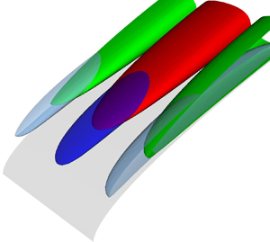
  $x\text {--}z$ plane, which have similar gains due to the small interaction between both sides of the body. Numerical errors from spatial-temporal discretization, remaining transient effects (SSRM), or truncation of the time series (TRM) can generate small differences between cosine and sine modes and mask the distinction of symmetric and asymmetric modes. Here the distinction between these gains is negligible, and they effectively span an optimal subspace. Figure 11 shows the upper half-domain of the leading modes for different frequencies. Figure 12 shows suboptimal modes for
  $\omega =0$. Vectors describing the optimal subspace were chosen to better represent the symmetries of the problem.

Figure 10. Leading gain for the parabolic body: (a) gains as a function of frequency, (b,c) gain convergence with iteration count. Results from the SSRM using the Arnoldi algorithm in coloured lines, and results from the TRM with the power iteration algorithm in black. (a) Frequency dependency of gains. (b) Gain convergence for  $\omega =0.00$. (c) Gain convergence for
  $\omega =0.25$.

Figure 11. Real part of optimal force (red and green) and response modes (blue and grey) for the flow around a parabolic body. On each subplot, forces and responses in the  $x$ (a,c,e) and
  $y$ (b,d,f) directions are shown. Results for (a,b)
  $\omega =0.00$; (c,d)
  $\omega =0.13$; (e,f)
  $\omega =0.25$.

Figure 12. Same as figure 11 for optimal and suboptimal modes at  $\omega =0.00$. (a,b) Optimal mode. (c,d) First suboptimal modes. Forces and responses in the x direction (a,c,e,g,i) and y direction (b,d,f,h,j) are shown. (e,f) Second suboptimal modes. (g,h) Third suboptimal modes. (i,j) Fourth suboptimal modes.
Figure 13 shows a comparison of the integration time required by each method. For the SSRM, an integration of 140 time units was used for eliminating transient effects, with another  $40$ units required to compute resolvent modes for the desired set of frequencies. All integrations have thus the same time length. Note, however, that the time needed to characterise the frequency responses increases with the inverse of frequency resolution. The TRM shows increasing integration times for each iteration, reaching
  $\approx 3.5$ times the initial time integration length at the last iteration. This cost, however, does not scale with the frequency discretization, which is an advantage of the TRM.

Figure 13. Total integration time using the different approaches. Half-integer/integer values refer to the direct/adjoint runs.
4.3. Cost comparisons
In this section we compare the costs of performing resolvent analysis with the proposed approach and previous methods. A quantitative comparison to state-of-the-art matrix-forming methods and a qualitative comparison with previous matrix-free methods are presented.
Matrix-forming methods are particularly effective for low-dimensional systems and are ubiquitous in studies of one-dimensional (1-D) problems. Their cost, however, increases rapidly with the number of points, and typically cannot by applied to three-dimensional (3-D) flows. We thus use the two-dimensional (2-D) flow over the same parabolic body considered in the previous sections. Compared with the 3-D case reported in § 4.2, the mesh was considerably refined, using  $112\times 38$ seventh-order spectral elements. The transient time used is the same as used in § 4.2.
The method was compared with a matrix-forming method obtained using a high-order finite difference method for the construction of a sparse matrix  $\boldsymbol{\mathsf{A}}$. The matrix-forming code has been extensively validated and used (e.g. Rodríguez, Gennaro & Souza (Reference Rodríguez, Gennaro and Souza2021) and references therein); the numerical details can be found in Gennaro et al. (Reference Gennaro, Rodríguez, Medeiros and Theofilis2013) and Rodríguez & Gennaro (Reference Rodríguez and Gennaro2017). Two approaches were used. In the first one, an eigenvalue-based ROM was constructed and gains obtained from it, similar to the approaches used by Åkervik et al. (Reference Åkervik, Ehrenstein, Gallaire and Henningson2008) and Alizard et al. (Reference Alizard, Cherubini and Robinet2009). In the second approach, an iterative method was also used, solving the linear problems (2.2a,b) and (2.8a,b), one frequency at a time. The linear problem is solved using the open-source sparse linear algebra package MUMPS (multifrontal parallel solver – Amestoy, Davis & Duff Reference Amestoy, Davis and Duff1996). Prior to the LU factorization, row ordering is applied using METIS (Karypis & Kumar Reference Karypis and Kumar1998). This approach is similar to the one used by Sipp & Marquet (Reference Sipp and Marquet2013) and Schmidt et al. (Reference Schmidt, Towne, Rigas, Colonius and Brès2018). The 2-D problem was discretized using a grid with
  $900\times 301$ points resulting in approximately
  $272\, 000$ grid points, roughly the same number of grid points used for the proposed approach.
The eigenmode-based ROM was constructed using 4000 eigenmodes, and 100 iterations were computed using the matrix-forming iterative method. With the SSRM, 10 iterations were computed for 26 frequencies simultaneously, resulting in a total of 260 frequency iterations. Note that since the SSRM performs iterations simultaneously for all the frequencies, the iteration count will be determined by the frequency with the slowest convergence rate. To compensate this, a higher iteration count was used with the SSRM.
The wall time and memory requirement of each method are reported in table 2. The costs for the 3-D problem studied in § 4.2 is added as reference. Note that the costs for the 3-D and 2-D problems scale roughly linearly with the number of grid points, which is a feature of the Nek5000's scalability and of the low added costs of the method, as discussed in the end of § 2.4.
Table 2. Wall time and memory requirement comparisons between the SSRM and matrix-forming methods for the 2-D problem discretized with  $\approx 272$ thousand grid points (
 $0.5$ million DOF). The values in parenthesis correspond to the 3-D problem described in § 4.2, with
  $\approx 1.5$ grid points (
 $4.5$ million DOF).

The proposed method obtained the results faster than the benchmarks, with a considerably lower memory requirement. It is worth mentioning that a direct comparison between the approaches is not straightforward. Reduced-order models based on eigenmodes can be effective (Lesshafft et al. Reference Lesshafft, Semeraro, Jaunet, Cavalieri and Jordan2019) or show an extremely low convergence rate (Alizard et al. Reference Alizard, Cherubini and Robinet2009), and the scaling of sparse matrix methods is problem dependent. The costs of the proposed approach depend not only on the relaxation time of the transient effects, which is problem dependent, but also on details of the solver used. Nevertheless, table 2 illustrates that memory requirements of matrix-forming methods can be prohibitive in applications to complex 3-D flows.
Comparing with the matrix-free method proposed by Monokrousos et al. (Reference Monokrousos, Åkervik, Brandt and Henningson2010), the SSRM has roughly the same cost, i.e. the costs associated with the time stepping of the linear system, but provides modes and gains for several frequencies simultaneously: if  $n_\omega$ frequencies are desired then the SSRM is approximately
  $n_\omega$ times cheaper. Assuming
  $n_\omega > 10$, total costs can be reduced by more than an order of magnitude, making the method comparable to the preconditioned approach used by Brynjell-Rahkola et al. (Reference Brynjell-Rahkola, Tuckerman, Schlatter and Henningson2017), but contrary to the latter, the present method is not limited to cases with low Reynolds numbers. As an improvement on the method of Monokrousos et al. (Reference Monokrousos, Åkervik, Brandt and Henningson2010), Gómez et al. (Reference Gómez, Sharma and Blackburn2016b) used lower accuracy solutions for the first iterations and an initial condition based on the current estimation of optimal force/response modes to reduce the total computational costs by
  $\approx 80\,\%$. The approach, however, recovers only the leading gains and modes, and has higher cost than the SSRM approach for
  $n_\omega >5$.
5. Conclusions
With the rising popularity of the resolvent analysis framework for modelling turbulent flows, several methods for obtaining optimal forcing and response modes have been proposed. The construction of full matrices describing the problem using spectral and pseudo-spectral methods are ubiquitous in 1-D problems. For 2-D problems, the approach can be extended by using high-order finite difference schemes and tools developed for manipulation of sparse matrices. However, these approaches are typically limited to simple geometries and become too expensive for 3-D problems. For complex, higher-dimensional problems, matrix-free methods are the natural choice.
In this study two novel methods that allow the computation of gains and modes for several frequencies simultaneously were presented. The TRM allows for a fine frequency discretization in the computation of leading modes and gains. The SSRM allows suboptimal gains and modes to be computed with the use of the Arnoldi algorithm. When implemented on an existing solver, the computation costs added scale linearly with the number of DOF, allowing for their use in virtually any problem for which the Navier–Stokes equations can be integrated.
The methods were validated in a linearized Ginzburg–Landau system, for which a direct SVD can be obtained and used as a benchmark. Geometric convergence rates with the number of iterations performed were observed with the proposed methods. As expected from analytical results presented in Appendix A, the convergence rates for the power iteration algorithm are proportional to the ratio of the first and second singular value. The Arnoldi algorithm provides suboptimal modes and an accelerated convergence rate, particularly when there is a small gain separation.
Gains and modes for the flow around a parabolic body were computed using an open-source implementation of the proposed methods within the Nek5000 code. When compared with a state-of-the-art matrix-forming tool (Rodríguez & Gennaro Reference Rodríguez and Gennaro2017; Rodríguez et al. Reference Rodríguez, Gennaro and Souza2021), the proposed approaches require similar CPU time but a fraction of the memory. When applied to the 3-D problem with  $4.5$ million DOF, the increase in costs of the proposed method is roughly proportional to the increase in the number of DOF. For this configuration, the application of the matrix-forming tools is unfeasible. Compared with other matrix-free methods (Monokrousos et al. Reference Monokrousos, Åkervik, Brandt and Henningson2010; Gómez et al. Reference Gómez, Sharma and Blackburn2016b; Brynjell-Rahkola et al. Reference Brynjell-Rahkola, Tuckerman, Schlatter and Henningson2017), the current approach has considerably lower costs when computation of several frequencies is required.
Funding
A.V.G.C. was supported by CNPq grant 310523/2017-6. E.M. acknowledges financial support by CAPES grant 88881.190271/2018-01. A.T. was supported in part by a catalyst grant from the Michigan Institute for Computational Discovery and Engineering (MICDE). The work of D.R. is funded by the Government of the Community of Madrid within the multi-annual agreement with Universidad Politécnica de Madrid through the Program of Excellence in Faculty (V-PRICIT line 3) and the Program of Impulse of Young Researchers (V-PRICIT line 1, grant number APOYO-JOVENES-WYOWRI-135-DZBLJU).
Declaration of interests
The authors report no conflict of interest.
Appendix A. Algorithms
Here, an overview of the iterative algorithms used in this work to compute singular values is presented. We focus on practical aspects that will be necessary for the development of the codes and methods used. For a more complete review of algorithms applicable to large systems, we refer the reader to Saad (Reference Saad2003).
The leading singular value and associated modes can be obtained via the power iteration algorithm, for which convergence can be easily derived analytically. First, define a test vector
 \begin{equation} \hat{\boldsymbol{f}}_0 = \sum_{i=1}^{{\boldsymbol{n}}_f} a_i \hat{{\boldsymbol{\mathcal{V}}}}_i. \end{equation}
Using (2.2a,b) and (2.8a,b) to form an iterative scheme,
 \begin{equation} \hat {\boldsymbol{w}}_n= (\boldsymbol{\mathsf{R}}_{{\boldsymbol{y}}}^{{{\dagger}}} \boldsymbol{\mathsf{R}}_{{\boldsymbol{y}}}) \hat {\boldsymbol{f}}_n \end{equation}
and choosing  $\hat {\boldsymbol {f}}_n = \hat {\boldsymbol {w}}_{n-1}$, for non-zero
  $a_1$, the term
  $\hat {\boldsymbol {f}}_n$ can be written as
 \begin{equation} \hat {\boldsymbol{f}} _{n}= (\boldsymbol{\mathsf{R}}_{{\boldsymbol{y}}}^{{{\dagger}}} \boldsymbol{\mathsf{R}}_{{\boldsymbol{y}}})^{n} \hat {\boldsymbol{f}}_0 = \boldsymbol{\mathsf{V}} \boldsymbol{\varSigma}^{2n} \boldsymbol{\mathsf{V}}^{{{\dagger}}} \hat {\boldsymbol{f}}_0 = a_1 \sigma_1^{2n} \left( {\boldsymbol{\mathcal{V}_1}} + \sum_{i=2}^{{\boldsymbol{n}}_f} \frac{a_i}{a_1}\frac{\sigma_i^{2n}}{\sigma_1^{2n}} {{\boldsymbol{\mathcal{V}}}}_i\right). \end{equation}
Assuming that  $\sigma _1 > \sigma _2$, for large
  $n$,
$n$,  $\hat {\boldsymbol {f}}_n/\sigma _1^{2n} \to {\boldsymbol {\mathcal {V}}}_{1}$, i.e. it converges to the leading force mode, and the leading gain can be estimated as
 \begin{equation} \sigma_{1,n}(\omega) = \sqrt\frac{\| \hat {\boldsymbol{f}}_ n(\omega)\| } {\| \hat {\boldsymbol{f}}_{n-1}(\omega)\| }. \end{equation}
Asymptotically, the power iteration algorithm has a geometrical convergence rate, with error reducing by a factor of  $(\sigma _1/\sigma _{2})^{2}$ on each iteration. In general,
  $\hat {\boldsymbol {f}}_n$ converges to the subspace spanned by the first
  $m$ force modes with a rate given by
  $\sigma _m/\sigma _{m+1}$. This is particularly relevant if
  $\sigma _1=\dots =\sigma _m$. In such case
  $\hat {\boldsymbol {f}}_n$ converges to one singular mode in the
  $m$-dimensional subspace, with rate
  $\sigma _1/\sigma _{m+1}$. This ratio will be referred to as gain separation.
If gain separation is small, i.e. close to 1, many iterations might be needed for convergence of the power iteration algorithm. Alternatively, gains can be estimated based on a low-rank representation of  $( \boldsymbol{\mathsf{R}}_{{\boldsymbol {y}}}^{{\dagger} } \boldsymbol{\mathsf{R}}_{{\boldsymbol {y}}} )$ in the subspace spanned by a sequence of vectors
  $\hat {\boldsymbol {f}}_n$, with
  $1\le n \le m$. We consider a set of vectors
  $\hat {\boldsymbol {f}}_n$ and
  $\hat {\boldsymbol {w}}_n$ that satisfy
 \begin{equation} (\boldsymbol{\mathsf{R}}_{{\boldsymbol{y}}}^{{{\dagger}}} \boldsymbol{\mathsf{R}}_{{\boldsymbol{y}}} )\hat {\boldsymbol{f}}_n = \hat {\boldsymbol{w}}_n, \end{equation}
where  $\hat {\boldsymbol {f}}_n$ are considered as inputs and
  $\hat {\boldsymbol {w}}_n$ as outputs. Using
  $\hat {\boldsymbol {f}}_n=\hat {\boldsymbol {w}}_{n-1}$, the subspace spanned by
  $\hat {\boldsymbol {f}}_n$ is the Krylov subspace. From (A3), it is clear that, for large
  $n$, this subspace asymptotically includes the leading force mode. Defining
  $\boldsymbol{\mathsf{F}} = [ \hat {\boldsymbol {f}}_1, \ldots , \hat {\boldsymbol {f}}_n ]$ and
  $\boldsymbol{\mathsf{W}} = [ \hat {\boldsymbol {w}}_1, \ldots ,\hat {\boldsymbol {w}}_n ]$, (A5) can be written as
 \begin{equation} (\tilde{\boldsymbol{\mathsf{R}}}_{{\boldsymbol{y}}}^{{{\dagger}}} \tilde{\boldsymbol{\mathsf{R}}}_{{\boldsymbol{y}}}) \tilde{\boldsymbol{\mathsf{F}}} = \tilde{\boldsymbol{\mathsf{W}}}, \end{equation}
where  $\tilde {\boldsymbol{\mathsf{F}}} = \boldsymbol{\mathsf{W}}_f^{1/2} \boldsymbol{\mathsf{F}}$,
  $\tilde {\boldsymbol{\mathsf{W}}} = \boldsymbol{\mathsf{W}}_f^{1/2} \boldsymbol{\mathsf{W}}$ and
  $\tilde {\boldsymbol{\mathsf{R}}}_{{\boldsymbol {y}}}=\boldsymbol{\mathsf{W}}_y^{1/2} \boldsymbol{\mathsf{R}}_{{\boldsymbol {y}}} \boldsymbol{\mathsf{W}}_f^{-1/2}$. From a QR decomposition,
  $\tilde {\boldsymbol{\mathsf{F}}}=\boldsymbol{\mathsf{Q}}_{\tilde {F}}\boldsymbol{\mathsf{R}}_{\tilde {F}}$, where
  $\boldsymbol{\mathsf{Q}}_{\tilde {F}}$ is a unitary matrix and
  $\boldsymbol{\mathsf{R}}_{\tilde {F}}$ is upper triangular, (A6) can be rewritten as
 \begin{equation} (\tilde{\boldsymbol{\mathsf{R}}}_{{\boldsymbol{y}}}^{{{\dagger}}} \tilde{\boldsymbol{\mathsf{R}}}_{{\boldsymbol{y}}}) \boldsymbol{\mathsf{Q}}_{\tilde{F}} = \tilde{\boldsymbol{\mathsf{W}}} \boldsymbol{\mathsf{R}}_{\tilde{F}}^{{-}1} = \boldsymbol{\mathsf{Q}}_{\tilde{F}} \underbrace{\boldsymbol{\mathsf{Q}}_{\tilde{F}}^{H} \tilde{\boldsymbol{\mathsf{W}}} \boldsymbol{\mathsf{R}}_{\tilde{F}}^{{-}1}}_{\boldsymbol{\mathsf{H}}} + \left(\boldsymbol{\mathsf{I}} -\boldsymbol{\mathsf{Q}}_{\tilde{F}}\boldsymbol{\mathsf{Q}}_{\tilde{F}}^{H} \right)\tilde{\boldsymbol{\mathsf{W}}} \boldsymbol{\mathsf{R}}_{\tilde{F}}^{{-}1}. \end{equation}
Since  $\boldsymbol{\mathsf{Q}}_{\tilde {F}}$ forms an orthonormal basis for the space spanned by
  $\boldsymbol{\mathsf{W}}_f^{1/2} \hat {\boldsymbol {f}}_n$, a low-rank representation of
  $(\tilde {\boldsymbol{\mathsf{R}}}_{{\boldsymbol {y}}}^{{\dagger} } \tilde {\boldsymbol{\mathsf{R}}}_{{\boldsymbol {y}}})$ in this space is given by
 \begin{equation} \boldsymbol{\mathsf{Q}}_{\tilde{F}}^{H}(\tilde{\boldsymbol{\mathsf{R}}}_{{\boldsymbol{y}}}^{{{\dagger}}} \tilde{\boldsymbol{\mathsf{R}}}_{{\boldsymbol{y}}}) \boldsymbol{\mathsf{Q}}_{\tilde{F}} = \boldsymbol{\mathsf{H}}, \end{equation}
where  $\boldsymbol{\mathsf{Q}}_{\tilde {F}}^{H} \boldsymbol{\mathsf{Q}}_{\tilde {F}} = \boldsymbol{\mathsf{I}}$ was used. The components of
  $\hat {\boldsymbol {f}}_n$ orthogonal to this space are restricted to the rightmost term. The eigenvalues and vectors of
  $(\tilde {\boldsymbol{\mathsf{R}}}_{{\boldsymbol {y}}}^{{\dagger} } \tilde {\boldsymbol{\mathsf{R}}}_{{\boldsymbol {y}}})$ can then be estimated from an eigen-decomposition of
  $\boldsymbol{\mathsf{H}}$,
 \begin{equation} \boldsymbol{\mathsf{H}} {\boldsymbol{\varPsi}} = \boldsymbol{\varGamma}^{2} {\boldsymbol{\varPsi}}, \end{equation}
where  $\boldsymbol {\varGamma }$ is diagonal with entries
  $\gamma _1\ge \gamma _2\ge \dots \ge \gamma _m$, and
  ${\boldsymbol {\varPsi }}$ is unitary, with the
  $j$th column represented by
  ${\boldsymbol {\psi }}_j$. Force and response modes, and gains associated with them, can be estimated as
 \begin{equation} {{\boldsymbol{\mathcal{V}}}}_{i} = \boldsymbol{\mathsf{Q}}_{F} {\boldsymbol{\psi}}_{i}, \quad {{\boldsymbol{\mathcal{U}}}}_{i} = \gamma_{i}^{{-}1}\boldsymbol{\mathsf{R}}_{{\boldsymbol{y}}} \boldsymbol{\mathsf{Q}}_{F} {\boldsymbol{\psi}}_{i}, \quad {\sigma}_{i} = \gamma_{i}. \end{equation}
 If  $\hat {\boldsymbol {f}}_n=\hat {\boldsymbol {w}}_{n-1}$, the rightmost term can be shown to have rank one, (A7) is an Arnoldi factorization of
  $(\tilde {\boldsymbol{\mathsf{R}}}_{{\boldsymbol {y}}}^{{\dagger} } \tilde {\boldsymbol{\mathsf{R}}}_{{\boldsymbol {y}}})$, and the matrix
  $\boldsymbol{\mathsf{H}}$ is Hessenberg and Hermitian. For large
  $n$,
$n$,  $\hat {\boldsymbol {f}}_n$ approximates the leading force mode, and, thus, the last vectors in the sequence become approximately linearly dependent. This leads to an ill-conditioning of the inversion of
  $\boldsymbol{\mathsf{R}}_{\tilde {F}}$. To avoid this problem, the Arnoldi algorithm can be used. It consists of using as
  $\hat {\boldsymbol {f}}_n$ the component of
  $\hat {\boldsymbol {w}}_{n-1}$ which is orthogonal to all previous forces
  $\hat {\boldsymbol {f}}_j$, with
  $j< i-1$. This can be obtained as
 \begin{equation} \hat {\boldsymbol{f}}_n = \hat {\boldsymbol{w}}_{n-1} - \boldsymbol{\mathsf{F}}_{0,\ldots,n-1} \hat{{\boldsymbol{\theta}}} , \end{equation}
where
 \begin{gather} \boldsymbol{\mathsf{F}}_{0,\ldots,n-1}=\left[\hat {\boldsymbol{f}}_0,\ldots,\hat {\boldsymbol{f}}_{n-1} \right], \end{gather}
 \begin{gather}\hat{{\boldsymbol{\theta}}}_i = \left( \boldsymbol{\mathsf{F}}^{H}_{0,\ldots,n-1} \boldsymbol{\mathsf{W}}_f \boldsymbol{\mathsf{F}}_{0,\ldots,n-1} \right)^{{-}1} \boldsymbol{\mathsf{F}}^{H}_{0,\ldots,n-1} \boldsymbol{\mathsf{W}}_f \hat {\boldsymbol{w}}_{n-1}. \end{gather}
 Note, however, that such ill-posedness only occurs once  $\hat {\boldsymbol {f}}_n$ has converged to the leading force mode; thus, if only the leading gain and modes are of interest, either the inversion of
  $\boldsymbol{\mathsf{R}}_{\tilde {F}}$ is well conditioned, or the leading modes and gains can be accurately obtained from the power iteration algorithm. The use of the Arnoldi algorithm is therefore only necessary if suboptimal gains and modes are of interest. Figure 14 reproduces figure 8 adding the trend observed with the Krylov algorithm. Krylov-subspace has the same convergence trend as the Arnoldi algorithm for the first iterations, and accurately captures the optimal gain before the algorithm becomes ill conditioned, and, thus, is a viable alternative to accelerate the computation of the leading mode if convergence rates are low due to small gain separations.


Appendix B. Temporal filter overview
Finite impulse response filters are a class of filters that can be applied to uniformly spaced time sequences. Given a signal sampled  $x(j \Delta t )$ and a filter
  $\phi (j \Delta t)$, the filtered signal
  $x'(j \Delta t)$ is obtained as
 \begin{equation} x' = \phi * x, \end{equation}
where  $*$ is a discrete convolution. In the frequency domain the filtered signal can be expressed as
 \begin{equation} \hat x' = \hat \phi \hat x. \end{equation}
If  $\phi$ is bounded, that is
  $\phi (t)=0$ for sufficiently large
  $|t|$, the filter is a FIR filter. The filter order is related to the number of points at which
  $\phi (j \Delta t)$ is non-zero: a
  $n$th order filter has
  $n+1$ non-zero points. Higher-order filters have better frequency resolution, with low-order filters having resolution only for frequencies close to the Nyquist frequency,
  $\omega _{nyq} = {\rm \pi}/(\Delta t)$.
Figure 15 shows an example of spectral flattening. Finite impulse response filters obtained with Matlab function fir2 are used to flatten the spectral content of  $x(t)=1/(t^{2}+1)$. The filter gain is chosen as
  $1/|\hat x(\omega )|$ for
  $\omega <{\rm \pi}$, smoothly going to zero at higher frequencies: this is the approach used in the TRM to regularize the problem and reduce aliasing effects. It can be seen that a filter with too low order has a poor performance, with the spectra of the filtered signal not being flat in the frequency range of interest, as illustrated in figure 15(a,b). Better performance is obtained with high-order filters, as can be seen in figures 15(c,d) and 15(e,f). The observed signal delay is given by
  $n_f \Delta t /2$ and is a consequence of the filters that are obtained with the fir2 function. These delays are compensated by timeshifting the signal.

Figure 15. Spectral flattening of the signal  $x$ using different filter orders resulting in the signals
  $x'$. Time and frequency-domain representations of the signal are shown, respectively, in the (a,c,e) and (b,d,f). Results for (a,b)
  $n_f=6$; (c,d)
  $n_f=50$; (e,f)
  $n_f=100$.
The frequency resolution of a FIR filter is proportional to  $\Delta T / n_f$. Figure 16 shows results using the same filter order as figure 15, but with a sampling rate five times higher, i.e.
  $\Delta T$ and frequency resolution five time larger. In this case, the spectra are successfully flattened only when higher-order filters are used. This highlights the importance of the cut-off frequency for TRM, as discussed in § 2.4, as the use of high frequencies increases not only storage requirement, but also the cost of signal filtering.

Figure 16. Same as 15, with a sampling rate five times higher. Results for (a,b)  $n_f=6$; (c,d)
  $n_f=50$; (e,f)
  $n_f=100$.
Appendix C. Interpolation algorithms and their spectral properties
For the TRM, described in § 2.2, simulation checkpoints need to be saved to disk for later use as an external force. As saving all time steps can require large storage, interpolation between different time steps is typically necessary. Three different interpolation methods between flow snapshots are investigated, and named after their smoothness:
(i)
 $C^{0}$: linear interpolation;
(ii)
$C^{1}$: cubic interpolation; and(iii)
$C^{2}$: fifth-order interpolation.


For the  $C^{0}$ interpolation method, coefficients of a first-order polynomial are chosen to match the function value at the interval limits. For the
  $C^{1}$ method, coefficients of a cubic polynomial are chosen to match desired values and first derivatives at the interval limits, with the derivatives estimated via a second-order finite difference scheme. Finally, for the
  $C^{2}$ method, coefficients of a fifth-order polynomial are chosen to match values up to the second derivatives at the interval limits, with first and second derivatives obtained with a five-point centred scheme. At the edges, the following are used:
(i)
$C^{1}$: first-order non-centred differentiation is used at the edge points;(ii)
$C^{2}$: second-order centred differentiation scheme is used to compute the first and second derivatives.


For the  $C^{2}$ interpolation, a first-order non-centred differentiation is used for the first derivative at the edge points, with the second derivative set to zero. The lower accuracy obtained at the edges has a limited impact on the method, as in these regions forcing and responses have vanishingly small amplitudes, so the absolute errors introduced are not relevant.
Figure 17 shows the performance of each approach for the interpolation of a sinusoidal signal, which reflects errors expected in the Fourier components of the signal. Figure 18 presents errors associated with each method, and figure 19 shows the spectral content of the interpolated functions. This parameter is important as large errors in the first harmonic create an artificial increase/decrease of resolvent gains. To obtain errors of the order  $10^{-2}$, approximately 4.5 points per cycle should be used. Interpolated signals with
  $n$ points per cycle are seen to generate the first spurious frequency peak at a frequency
  $n-1$ times the frequency of the original signal.

Figure 17. Interpolation of a sinusoidal signal with the three proposed methods. (a,c) Three points per cycle. (b,d) Four points per cycle.

Figure 18. Interpolation error norm, and error of the first Fourier coefficient. (a) Error norm. (b) First harmonic error.

Figure 19. Spectral content of the interpolated signals. (a) Interpolation leakage using 2.5 points per cycle. (b) Interpolation leakage using 4.0 points per cycle.
Appendix D. Code validation
The ‘Nek5000 resolvent tools’ package uses the Nek5000 open-source code for the integration of the linearized direct and adjoint Navier–Stokes equations. The package is validated on a channel flow with a Reynolds number 50, based on the centreline velocity and the channel half-width, for 2-D and 3-D configurations. Domain lengths of  $4{\rm \pi}$ in the streamwise direction and
  $0.01$ in the spanwise directions, for 3-D simulations, were used, with periodic conditions in the streamwise and spanwise directions. With such a narrow spanwise length, the dominant spanwise wavenumber is
  $\beta =0$ at all frequencies. Results obtained with 20 iterations using the code were compared against standard tools based on the decomposition of perturbations in spanwise and streamwise wavenumbers, previously used by Nogueira et al. (Reference Nogueira, Morra, Martini, Cavalieri and Henningson2021). Wavenumbers were looped over to search for the dominant gains at each frequency.
Figure 20 compares the gains obtained with the explicit construction of the system matrices with those obtained with the implementation of the matrix-free method described in this work. Both approaches produce the same gains, validating the current implementation to two- and three-dimensional problems. Files for reproducing the validation of these results are available in the ‘examples’ branch of the Git repository at https://github.com/eduardomartini/Nek5000_ResolventTools.

Figure 20. Code validation on a laminar channel flow. Gains obtained with explicit construction of the system matrices (back lines) are closely matched by those obtained with the open-source code (coloured lines). (a) Two dimensions; (b) three dimensions.


