


1. Introduction
The breakup of electrohydrodynamically driven capillary jets has attracted significant attention since it is crucial to a range of micro-nano manufacturing technologies, such as electrohydrodynamic (EHD) jet printing (Onses et al. Reference Onses, Sutanto, Ferreira, Alleyne and Rogers2015; Yin et al. Reference Yin, Huang, Bu, Wang and Xiong2010), nano-powder production (Jaworek, Sobczyk & Krupa Reference Jaworek, Sobczyk and Krupa2018) and drug delivery (Bhardwaj & Kundu Reference Bhardwaj and Kundu2010). In these applications, a fine EHD jet is issued from a so-called Taylor cone when a strong electric field is applied to a dripping liquid. Several regimes regarding the flow rate and electric field intensity in EHD flows have been demarcated, and the steady cone-jet mode is the most useful one (Onses et al. Reference Onses, Sutanto, Ferreira, Alleyne and Rogers2015). In the cone-jet mode, the cone remains unchanged, whereas the downstream jet breaks into small drops. Although many experimental, theoretical and numerical studies have investigated the steady cone jet and EHD jet breakup under specific conditions (Fernández de la Mora Reference Fernández de la Mora2007; Gañán-Calvo et al. Reference Gañán-Calvo, López-Herrera, Herrada, Ramos and Montanero2018; Rosell-Llompart, Grifoll & Loscertales Reference Rosell-Llompart, Grifoll and Loscertales2018), it is still challenging to understand the pinching mechanism of such an electrified jet, especially in conditions beyond the perfectly conducting limit.
Pinching of an electrified jet involves capillary instability induced by surface tension and coulombic instability induced by the surface charge. For capillary instability, the pioneers Plateau (Reference Plateau1857) and Rayleigh (Reference Rayleigh1878) demonstrated that, when ignoring the effect of the surrounding air, an uncharged inviscid filament with a radius of  ${\bar{r}_0}$ is unstable to suffer a long-wavelength disturbance
  $\bar{\lambda } > {\bar{\lambda }_{crit}} = 2\pi{\bar{r}_0}$ and encounters a maximum growing mode with a wavelength
  ${\bar{\lambda }_{max}} = 9.01{\bar{r}_0}$ (or wavenumber
  ${\bar{k}_{max}} = 0.697/{\bar{r}_0}$). In this paper, all the variables with bars are dimensional. The theoretical framework is extended to viscous jets and the nonlinear analysis of higher-order perturbations, and is confirmed by sufficient experimental observations and high-accuracy computations (Eggers Reference Eggers1997; Eggers & Villermaux Reference Eggers and Villermaux2008).
When a jet is electrified or charged, the breakup dynamics is complex because surface charges destabilize the jet, even in the absence of axial perturbations. Rayleigh (Reference Rayleigh1882) examined the instability of a charged, inviscid liquid cylindrical column, and showed that the cylinder yields the instability condition  $\bar{Q} > \sqrt {6\pi{{\bar{\varepsilon }}_0}\bar{\gamma }\bar{r}} $, where
  $\bar{Q}$ is the charge density per unit length,
  $\bar{\gamma }$ the surface tension and
  ${\bar{\varepsilon }}$ is the vacuum permittivity. Based on Rayleigh's work, Basset (Reference Basset1894) studied the dynamics of a charged cylinder subjected to an axisymmetric disturbance using linear analysis, and demonstrated that the charge widens the range of unstable wavenumbers and stabilizes the jet for a long-wave disturbance while destabilizing it for a short-wave disturbance. Furthermore, Bassett reported that charges destabilize non-axisymmetric deformations, which was also discussed in the theoretical analysis by Huebner & Chu (Reference Huebner and Chu1971). Saville (Reference Saville1971a) considered viscosity and found that the viscous effect dampened the axisymmetric motions and rendered the non-axisymmetric motions more unstable. The axisymmetric and non-axisymmetric motions are also called varicose and kink instabilities in experimental observations (Yang et al. Reference Yang, Duan, Li and Deng2014a). The above studies either considered a charged jet in the absence of a tangential electric field or treated the jet as a perfect conductor. Under such a perfectly conducting limit, the charge can relax onto the jet interface instantaneously or the jet surface is equipotential. Besides, the jet interface is only acted upon by the normal stress. Saville (Reference Saville1971b) investigated a weakly conducting jet in a tangential electric field and reported that the charge relaxation could cause oscillatory growth of a perturbation. Mestel (Reference Mestel1994, Reference Mestel1996) extended Saville's analysis and discussed the effects of both the surface charge and the tangential electric field on the EHD stability of viscous jets. He noted that shear stresses can suppress capillary instability. Artana, Romat & Touchard (Reference Artana, Romat and Touchard1998) considered the non-isopotential case and theoretically analysed the linear stability of an electrified jet in a coaxial electrode. López-Herrera, Riesco-Chueca & Gañán-Calvo (Reference López-Herrera, Riesco-Chueca and Gañán-Calvo2005) consulted a general physical model similar to that of Artana et al. but incorporated the influences of the electrode radius, the surrounding air and the viscous boundary layer on the jet instability. Moreover, the authors deduced a complete dispersion relation for a weakly conducting jet.
Linear stability analysis can provide the parameter space for stable or unstable jets but cannot describe the characteristics during long-term evolution, such as the formation of satellite drops. Setiawan & Heister (Reference Setiawan and Heister1997) first modelled the nonlinear dynamics of an inviscid, electrified jet using the boundary element method (BEM). They discussed how the nonlinear contributions affect the main and satellite drop sizes in the pinch-off region. López-Herrera, Gañán-Calvo & Perez-Saborid (Reference López-Herrera, Gañán-Calvo and Perez-Saborid1999) used one-dimensional simulations based on slender approximation equations to investigate the effects of electric stress and viscosity on the drop formation from a pinching jet. Based on the work of Setiawan & Heister (Reference Setiawan and Heister1997) and López-Herrera, Gañán-Calvo & Perez-Saborid (Reference López-Herrera, Gañán-Calvo and Perez-Saborid1999), Collins, Harris & Basaran (Reference Collins, Harris and Basaran2007) comprehensively studied the breakup times, the ratios of the sizes of the primary to satellite drops formed at pinch-off and the coulombic stability of the drops using one- and two-dimensional simulations. The authors demonstrated the electric stress significantly increases the size of satellite drops. In contrast to the study by Collins et al., Wang & Papageorgiou (Reference Wang and Papageorgiou2011) investigated the touchdown in the jet breakup using BEM. These studies only considered cases in the perfectly conducting limit. Wang (Reference Wang2012) later analysed a poorly conducting Stokes jet suspended in a viscous, dielectric medium and found that the satellite formation of this jet is different from that in the perfectly conducting case. The author argued that electric shear stress promotes the formation of multiple satellite drops. Li et al. (Reference Li, Ke, Yin and Yin2019) discussed the effect of finite conductivity on the nonlinear dynamics of a viscoelastic, weakly conducting liquid jet and concluded that the tangential stress prevented the formation of satellite drops in the beads-on-a-string structure.
There have been few experimental studies of the capillary breakup of a charged jet although the cone-jet mode and its subsequent breakup are found in numerous EHD applications. López-Herrera & Ganan-Calvo (Reference López-Herrera and Ganan-Calvo2004) experimentally studied the axisymmetric breakup of a weakly electrified jet from an orifice and showed a remarkable agreement with one-dimensional simulations. Yang et al. (Reference Yang, Duan, Li and Deng2014a) investigated the varicose and whipping instabilities of electrified jets to an axial direct current (DC) electric field and radial alternating current (AC) electric field. However, the strength of the radial electric field in the experiments of López-Herrera et al. and Yang et al. is smaller than the axial one and so the effect of electric stress on the varicose instabilities is not significant. Li et al. (Reference Li, Ke, Yin and Yin2019, Reference Li, Ke, Xu, Yin and Yin2020) conducted the radial deformation of an electrified jet by building a needle–cylinder electrode. The authors found spike structures, disk-like structures and tip streaming when the radial electric field is huge. Recently, Montanero & Gañán-Calvo (Reference Montanero and Gañán-Calvo2020) have comprehensively reviewed the breakup of electrified jets, as well as their linear stability.
The objective of this study is to expound on the effect of charge relaxation on the linear and nonlinear dynamics of an axisymmetric weakly conducting jet with arbitrary viscosities in a radial electric field. The electrical conductivity of this weakly conducting jet, which is also called a leaky-dielectric jet, is typically less than 10−9 S m−1; thus, the characteristic time for charge relaxation ( ${\bar{t}_e} = \bar{\varepsilon }/\bar{K}$, where
  $\bar{\varepsilon }$ and
  $\bar{K}$ are the electrical permittivity and conductivity, respectively) is comparable to the hydrodynamic time (Saville Reference Saville1997; Sengupta, Walker & Khair Reference Sengupta, Walker and Khair2017). Since the charge relaxation time is not zero, the electric field acting on the surface charge generates a tangential component of electric stress that requires tangential viscous stress to balance it. Melcher & Taylor (Reference Melcher and Taylor1969) reported that the interfacial shear stress could induce cellular convection when a leaky-dielectric fluid is subjected to a DC/AC electric field. In this case, the surface charge can also be transported by convection. Saville (Reference Saville1997) summarized the Taylor–Melcher leaky-dielectric model and formulated the surface charge conservation equation as follows:
 \begin{equation}\underbrace{{\frac{{\partial \bar{q}}}{{\partial \bar{t}}}}}_{{Charge\ accumulation}} + \underbrace{{\bar{\boldsymbol{u}}\boldsymbol{\boldsymbol{\cdot} }{{\bar{\nabla }}_s}\bar{q}}}_{{Charge\ convection}} - \underbrace{{\bar{q}\boldsymbol{n}\boldsymbol{\boldsymbol{\cdot} }(\boldsymbol{n}\boldsymbol{\boldsymbol{\cdot} }\bar{\boldsymbol{\nabla }})\bar{\boldsymbol{u}}}}_{{Interface\ dilation}} = \underbrace{{\bar{K}\bar{\boldsymbol{E}}\boldsymbol{\boldsymbol{\cdot} }\boldsymbol{n}}}_{{Ohmic\ conduction}},\end{equation}
where  $\bar{q}$ is the surface charge density,
  $\bar{\boldsymbol{u}}$ and
  $\bar{\boldsymbol{E}}$ are the velocity and electric field inside the liquid, respectively,
  ${\bar{\nabla }_s}$ is the surface gradient operator, and
  $\boldsymbol{n}$ is the outward pointing unit vector normal to the liquid surface. In the perfectly conducting limit, the charge accumulation, also called the charge relaxation (Sengupta et al. Reference Sengupta, Walker and Khair2017), is entirely contributed by ohmic conduction. If the electrical conductivity drops to 10−9 S m−1, the sum of charge convection and charge variation due to the interface dilation are comparable to the ohmic conduction. For convenience, the second and third terms on the left-hand side of (1.1) are collectively called the surface charge convection (Sengupta et al. Reference Sengupta, Walker and Khair2017). In the leaky-dielectric case, the pinching process of electrified jets is subjected to both normal and tangential electric stresses. Recently, several numerical and experimental studies have quantitatively demonstrated that surface charge convection plays an important role in the drop deformation (Lanauze, Walker & Khair Reference Lanauze, Walker and Khair2015; Sengupta et al. Reference Sengupta, Walker and Khair2017). It is noted that (1.1) is the standard surface charge conservation equation that can be derived from the electrokinetic theory when neglecting the terms of charge diffusion and chemical reaction (Saville Reference Saville1997). A few studies make further efforts to discuss the effects of surface conduction (Burton & Taborek Reference Burton and Taborek2011; Giglio et al. Reference Giglio, Rangama, Guillous and Le Cornu2020) or charged surfactants (Conroy et al. Reference Conroy, Matar, Craster and Papageorgiou2011). This paper limits the focus on the ohmic conduction and surface charge convection of (1.1) without additional terms and ignoring electrokinetic effects. Wang (Reference Wang2012) recognized the importance of the surface charge convection but did not explain how the charge relaxation affects the pinching process. Moreover, it seems that the tangential stresses in the studies of Wang (Reference Wang2012) and Li et al. (Reference Li, Ke, Yin and Yin2019) play opposite roles in satellite formation. Hence, the satellite drops affected by the tangential stresses are also of interest in this work. Capturing the jet surface at pinch-off requires high-resolution computations since the radius near the pinching point is several orders of magnitude smaller than the initial jet radius. Considerable investigations were conducted by Basaran's group using finite element methods (FEMs) to resolve the singularity in dripping (Ambravaneswaran, Phillips & Basaran Reference Ambravaneswaran, Phillips and Basaran2000), jetting and their transition (Ambravaneswaran et al. Reference Ambravaneswaran, Subramani, Phillips and Basaran2004). Collins et al. (Reference Collins, Harris and Basaran2007, Reference Collins, Jones, Harris and Basaran2008) have shown that FEM can accurately depict the capillary pinching of charged jets and tip streaming of electrified films using the elliptic mesh generation algorithm to track the moving boundary. This work adopts FEM to deal with the governing equations and uses an arbitrary Lagrangian–Eulerian (ALE) technique to track the jet surface since this method combines the advantages of the Lagrange and Euler methods (Yang, Hong & Cheng Reference Yang, Hong and Cheng2014b).
The rest of the paper is organized as follows. Section 2 presents the physical model, governing equations, boundary and initial conditions, as well as the numerical method. In § 3, comparisons of the pinching processes between the perfectly conducting and leaky-dielectric jets are performed. Section 4 expounds on the difference between the two kinds of jets using linear stability analysis and nonlinear dynamics. Concluding remarks are presented in § 5.
2. Problem description
2.1. Physical model
This study considers a leaky-dielectric liquid jet of length  ${\bar{Z}_0}$ and radius
  ${\bar{r}_0}$ flowing through a concentric cylindrical electrode of radius
  ${\bar{R}_0}$, as depicted in figure 1. A similar model was also described by Setiawan & Heister (Reference Setiawan and Heister1997) and Collins et al. (Reference Collins, Harris and Basaran2007) The liquid jet inside the domain
  ${\varOmega _L}$ is an incompressible Newtonian fluid with uniform density
  $\bar{\rho }$, dynamic viscosity
  $\bar{\mu }$, electrical permittivity
  $\bar{\varepsilon }$ and electrical conductivity
  $\bar{K}$ and is surrounded by a passively insulating gas
  $({\varOmega _G})$ of permittivity
  ${\bar{\varepsilon }_0}$. The liquid–gas interface is denoted by
  ${S_f}$ with a constant surface tension
  $\bar{\gamma }$. This work assumes the surrounding gas is motionless but provides a datum pressure on the liquid jet. Besides, the velocity boundary layer at the interface is not considered although it affects the jet instability (López-Herrera et al. Reference López-Herrera, Riesco-Chueca and Gañán-Calvo2005). Since the charge transportation is of interest in this work, the surface charge density at the interface is initialized to
  ${\bar{q}_0}$, and the electrode is grounded. The free surface is subjected to a cosine perturbation of magnitude
  ${\bar{A}_0}$ and axial wavelength
  $\bar{\lambda }$ (
 $\bar{\lambda } = 2\pi/\bar{k}$,
  $\bar{k}$ is the wavenumber) at
  $\bar{t} = 0$. A periodic condition is used along the
  $\bar{z}$-axis, and the electrode radius is maintained
  ${\bar{R}_0} = 10{\bar{r}_0}$ to exclude the effects of electrode geometry (Collins et al. Reference Collins, Harris and Basaran2007). The value
  ${\bar{Z}_0} = \lambda $ is chosen in the simulations. For an unperturbed jet, the initial condition of
  ${\bar{q}_0}$ is identical to that of an electrical potential
  ${\bar{\varPhi }_0} = {\bar{q}_0}{\bar{r}_0}\ln (\bar{R}/{\bar{r}_0})/{\bar{\varepsilon }_0}$ or a radial electric field
  ${\bar{E}_0} = {\bar{q}_0}/{\bar{\varepsilon }_0}$. The jet deposited by surface charges is called a charged jet, while that imposed by a constant potential is termed an electrified jet. Most studies do not distinguish between the two jets. Nevertheless, in a perturbed leaky-dielectric jet, only the initial condition
  ${\bar{q}_0}$ can generate a tangential electric field. This initial condition was addressed by López-Herrera & Ganan-Calvo (Reference López-Herrera and Ganan-Calvo2004) and was adopted by Wang (Reference Wang2012) and Li et al. (Reference Li, Ke, Yin and Yin2019).

Figure 1. Definition sketch of a perturbed, axisymmetric and charged jet. The dashed lines represent the quiescent jet at  $\bar{t} < 0$. The red plus signs and double arrows stand for the surface charge and fluid flow, respectively.
For a leaky-dielectric jet, the surface charge convection primarily depends on the hydrodynamic flows, which arise from the oscillation of the surface or the EHD flow. The time scales of the two flows are denoted as  ${\bar{t}_\gamma } = \sqrt {\bar{\rho }\bar{r}_0^3/\bar{\gamma }} $ and
  ${\bar{t}_f} = \bar{\mu }/(\bar{\varepsilon }\bar{E}_0^2)$, respectively (Saville Reference Saville1997). López-Herrera et al. (Reference López-Herrera, Riesco-Chueca and Gañán-Calvo2005) used the relaxation parameter
  $\alpha = {\bar{t}_\gamma }/{\bar{t}_e} = {[{\bar{K}^2}\bar{\rho }\bar{r}_0^3/({\bar{\varepsilon }^2}\bar{\gamma })]^{1/2}}$ to measure the importance of charge relaxation. When
  $\alpha \to \infty $, the ohmic conduction dominates the charge relaxation; thus, the charges tend to accumulate at the peaks and troughs (marked by four plus signs in figure 1) since the curvatures are the largest at these positions. An intuitive but extreme phenomenon is the point discharge. When
  $\alpha $ is finite, the transport of the charges to the peaks or troughs is as slow as the fluid flow (marked by red double arrows in figure 1), and the charges are redistributed at the interface.
2.2. Governing equations
The simulation of EHD breakup of leaky-dielectric jets requires the calculation of the fluid flow and the electric potential. Dimensional analysis is used to define the following variables as scales of the length, time, velocity, pressure, surface charge density and electric potential:
 \begin{equation}{\bar{r}_0},\quad \sqrt {\bar{\rho }\bar{r}_0^3/\bar{\gamma }} ,\quad {\bar{r}_0}/\sqrt {\bar{\rho }\bar{r}_0^3/\bar{\gamma }} ,\quad \bar{\gamma }/{\bar{r}_0},\quad {\bar{q}_0},\quad {\bar{\varPhi }_0}.\end{equation}
Consequently, the pinching process of leaky-dielectric jets is governed by the dimensionless Navier–Stokes (NS) equations
 \begin{gather}\frac{{\partial \boldsymbol{u}}}{{\partial t}} + \boldsymbol{u}\boldsymbol{\boldsymbol{\cdot} }\boldsymbol{\nabla }\boldsymbol{u} ={-} \boldsymbol{\nabla }p + Oh{\nabla ^2}\boldsymbol{u}\;\textrm{in}\;{\varOmega _L},\end{gather}
 \begin{gather}\boldsymbol{\nabla }\boldsymbol{\boldsymbol{\cdot} }\boldsymbol{u} = 0\;\textrm{in}\;{\varOmega _L},\end{gather}
and the dimensionless electrostatic equation
 \begin{equation}{\nabla ^2}\varPhi = 0\;\textrm{in}\;{\varOmega _L} \cup {\varOmega _G}.\end{equation}
The three equations are used to solve the velocity vector  $\boldsymbol{u}$ and pressure p inside the liquid jet and the electric potential
  $\varPhi $ in the entire space. Here,
  $Oh = \bar{\mu }/\sqrt {\bar{\rho }\bar{\gamma }{{\bar{r}}_0}} $ is the Ohnesorge number that relates the viscous forces to the inertial and surface tension forces. The NS equations are coupled with the electrostatic equation via the stress balance along
  ${S_f}$, which is defined as
 \begin{equation}\boldsymbol{n}\boldsymbol{\boldsymbol{\cdot} }[{\mathbb T}^{h} - {\mathbb T}^{e}]_L^G = \kappa \boldsymbol{n}\;\textrm{on}\;{S_f}.\end{equation}
The two terms in the square brackets are the hydrodynamic and Maxwell stresses across the liquid–gas interface, where  ${\mathbb T}^{h} ={-} p{\mathbb I} + Oh(\boldsymbol{\nabla }\boldsymbol{u} + {(\boldsymbol{\nabla }\boldsymbol{u})^\textrm{T}})$ and
  ${\mathbb T}^{e} = C{a_E}(\boldsymbol{EE} - {\boldsymbol{E}^2}{\mathbb I}/2)$, respectively. Here,
  ${\mathbb I}$ is the identity matrix and
  $\boldsymbol{E} ={-} \boldsymbol{\nabla }\varPhi$ is the electric field measured by
  ${\bar{E}_0} = {\bar{q}_0}/{\bar{\varepsilon }_0}$. The term on the right-hand side of (2.5) is the surface tension that is derived from the local mean curvature, which is computed by
  $\kappa ={-} (\boldsymbol{\nabla }\boldsymbol{\boldsymbol{\cdot} }\boldsymbol{n})$. Here,
  $C{a_E} = {\bar{\varepsilon }_0}\bar{E}_0^2{\bar{r}_0}/\bar{\gamma }$ is the electric capillary number that measures the electric to capillary stresses. In our model, the hydrodynamic stress inside the gas is zero, viz.,
  ${{\mathbb T}}_G^h = 0$. The subscripts L and G denote the liquid and gas domains, respectively.
On the jet surface, the electric field affects the charge distribution, which, in turn, modifies the electric field. It is defined by the dimensionless surface charge conservation equation derived from (1.1)
 \begin{equation}\frac{{\partial q}}{{\partial t}} + \boldsymbol{u} \boldsymbol{\cdot} {\nabla _s}q - q\boldsymbol{n}\boldsymbol{\boldsymbol{\cdot} }(\boldsymbol{n}\boldsymbol{\boldsymbol{\cdot} }\boldsymbol{\nabla })\boldsymbol{u} = \varepsilon \alpha {\boldsymbol{E}_L}\boldsymbol{\boldsymbol{\cdot} }\boldsymbol{n}\;\textrm{on}\;{S_f},\end{equation}
where q is the surface charge density computed by the Gauss law  $q = \boldsymbol{n}\boldsymbol{\boldsymbol{\cdot} }({\boldsymbol{E}_G} - \varepsilon {\boldsymbol{E}_L})$,
  $\varepsilon = \bar{\varepsilon }/{\bar{\varepsilon }_0}$ is the relative permittivity of the liquid jet. Reorganizing the term of surface charge convection as
 \begin{align}\begin{array}{ll} \boldsymbol{u} \boldsymbol{\cdot} {\nabla _s}q - q\boldsymbol{n}\boldsymbol{\boldsymbol{\cdot} }(\boldsymbol{n}\boldsymbol{\boldsymbol{\cdot} }\boldsymbol{\nabla })\boldsymbol{u} \!\!\!\!\!&= \boldsymbol{u} \boldsymbol{\cdot} {\nabla _s}q + q[\boldsymbol{\nabla }\boldsymbol{\boldsymbol{\cdot} }\boldsymbol{u} - \boldsymbol{n} \boldsymbol{\cdot} (\boldsymbol{n}\boldsymbol{\boldsymbol{\cdot} }\boldsymbol{\nabla })\boldsymbol{u}]\\ & = \boldsymbol{u} \boldsymbol{\cdot} {\nabla _s}q + q[\boldsymbol{\nabla } - (\boldsymbol{n}\boldsymbol{\boldsymbol{\cdot} }\boldsymbol{\nabla })\boldsymbol{n}]\boldsymbol{\boldsymbol{\cdot} }\boldsymbol{u}\\ & = \boldsymbol{u} \boldsymbol{\cdot} {\nabla _s}q + q{\nabla _s} \boldsymbol{\cdot} \boldsymbol{u} = {\nabla _s} \boldsymbol{\cdot} (q\boldsymbol{u}), \end{array}\end{align}
the dimensionless surface charge conservation equation is rewritten as
 \begin{equation}\frac{{\partial q}}{{\partial t}} + {\nabla _s} \boldsymbol{\cdot} (q\boldsymbol{u}) = \varepsilon \alpha {\boldsymbol{E}_L}\boldsymbol{\boldsymbol{\cdot} }\boldsymbol{n}\;\textrm{on}\;{S_f},\end{equation}
where  ${\nabla _s} = ({\mathbb I} - \boldsymbol{nn})\boldsymbol{\boldsymbol{\cdot} }\boldsymbol{\nabla }$ is the surface divergence operator. The appearance of
  $\boldsymbol{u}$ in (2.8) couples the electric field and the fluid flow, which satisfies the kinematic condition
 \begin{equation}\boldsymbol{n}\boldsymbol{\boldsymbol{\cdot} }(\boldsymbol{u} - {\boldsymbol{u}_s}) = 0\;\textrm{on}\;{S_f},\end{equation}
where  ${\boldsymbol{u}_s}$ is the local velocity on
  ${S_f}$. At the interface, the continuity of the tangential component
  $(\tau )$ of the electric field is given by
 \begin{equation}\boldsymbol{n} \times ({\boldsymbol{E}_G} - {\boldsymbol{E}_L}) = 0\;\textrm{on}\;{S_f},\end{equation}
i.e.  ${E_{L,\tau }} = {E_{G,\tau }} = {E_\tau }$. A comparison of (2.2), (2.4), (2.5) and (2.8) with the corresponding dimensional equations shows that
  $Oh$,
$Oh$,  $\varepsilon $,
  $C{a_E}$ and
  $\varepsilon \alpha $ represent the effects of the liquid viscosity, the permittivity, the electric intensity at the jet interface and the conductivity, respectively.
Initially, the jet surface is perturbed by a linear cosine disturbance in the form of  ${S_f} = 1 + {A_0}\cos (kz)$, where the initial perturbation
  ${A_0}$ equals to
  ${10^{ - 2}}$. It is noticed that
  ${A_0}$ and the perturbation form affect the breakup time but only slightly influence the jet pinching. The details are described in appendices A and B. At
  $t = 0$, the interface is charged with a constant surface charge density
  $q{|_{t = 0}} = 1$. On the electrode surface, the electric potential is
 \begin{equation}\varPhi = 0\;\textrm{at}\;r = 10.\end{equation}
Regarding the finiteness of the physical quantities at the symmetry axis, the radial components of the electric field and velocity satisfy
 \begin{equation}{E_r} = 0\quad \textrm{and}\quad {u_r} = 0\;\textrm{at}\;r = 0.\end{equation}
 This work considers an electrified jet whose properties are similar to the work fluids in EHD applications (Bhardwaj & Kundu Reference Bhardwaj and Kundu2010; Jaworek et al. Reference Jaworek, Sobczyk and Krupa2018; Onses et al. Reference Onses, Sutanto, Ferreira, Alleyne and Rogers2015). The jet has a radius of ~10 μm and is subjected to an electric field of  ${\sim} {10^6}\;\textrm{V}\;{\textrm{m}^{ - 1}}$; the magnitudes of the dimensionless numbers in the above descriptions are respectively
  $Oh\sim 1$,
  $C{a_E}\sim 1$,
  $\varepsilon \sim 10$ and
  $\alpha \sim 10$.
2.3. Numerical scheme
Equations (2.2)–(2.4) and (2.8) are solved by the FEM using mathematical models with so-called weak formulations. When (2.2) and (2.3) are integrated inside the liquid domain, and the Gauss divergence theorem is applied, the weak representations are defined as follows:
 \begin{align}0 &
= \int_{{\varOmega _L}} {\dfrac{{\partial
\boldsymbol{u}}}{{\partial
t}}\boldsymbol{\mathscr{u}}\,\textrm{d}{\varOmega _L}} +
\int_{{\varOmega _L}} {(\boldsymbol{u}\boldsymbol{\boldsymbol{\cdot}
}\boldsymbol{\nabla
}\boldsymbol{u})\boldsymbol{\mathscr{u}}\,\textrm{d}{\varOmega _L}} -
Oh\int_{{\varOmega _L}} {\boldsymbol{\nabla
}\boldsymbol{u}\boldsymbol{\nabla
}\boldsymbol{\mathscr{u}}\,\textrm{d}{\varOmega _L}} \nonumber\\
& \quad - \int_{{\varOmega _L}} {p\boldsymbol{\nabla
}\boldsymbol{\boldsymbol{\cdot} }\boldsymbol{\mathscr{u}}\,\textrm{d}{\varOmega
_L}} - \int_{{S_L}} {\left( {Oh\dfrac{{\partial
\boldsymbol{u}}}{{\partial \boldsymbol{n}}} -
p\boldsymbol{n}} \right)\boldsymbol{\boldsymbol{\cdot}
}\boldsymbol{\mathscr{u}}\,\textrm{d}{S_L}} ,
\end{align}
\begin{align}0 &
= \int_{{\varOmega _L}} {\dfrac{{\partial
\boldsymbol{u}}}{{\partial
t}}\boldsymbol{\mathscr{u}}\,\textrm{d}{\varOmega _L}} +
\int_{{\varOmega _L}} {(\boldsymbol{u}\boldsymbol{\boldsymbol{\cdot}
}\boldsymbol{\nabla
}\boldsymbol{u})\boldsymbol{\mathscr{u}}\,\textrm{d}{\varOmega _L}} -
Oh\int_{{\varOmega _L}} {\boldsymbol{\nabla
}\boldsymbol{u}\boldsymbol{\nabla
}\boldsymbol{\mathscr{u}}\,\textrm{d}{\varOmega _L}} \nonumber\\
& \quad - \int_{{\varOmega _L}} {p\boldsymbol{\nabla
}\boldsymbol{\boldsymbol{\cdot} }\boldsymbol{\mathscr{u}}\,\textrm{d}{\varOmega
_L}} - \int_{{S_L}} {\left( {Oh\dfrac{{\partial
\boldsymbol{u}}}{{\partial \boldsymbol{n}}} -
p\boldsymbol{n}} \right)\boldsymbol{\boldsymbol{\cdot}
}\boldsymbol{\mathscr{u}}\,\textrm{d}{S_L}} ,
\end{align}
and
 \begin{equation}0 = \int_{{\varOmega _L}} {(\boldsymbol{\nabla }\boldsymbol{\boldsymbol{\cdot} }\boldsymbol{u})\mathscr{p}\,\textrm{d}{\varOmega _L}} ,\end{equation}
where  $\boldsymbol{\mathscr{u}}$ and
  $\mathscr{p}$ are the test functions of the velocity vector
  $\boldsymbol{u}$ and pressure p, respectively. Here,
  ${\textrm{S}_L}$ represents the boundary of the liquid domain. In the same manner, the weak form of (2.4) is expressed as
 \begin{equation}0 = \int_\varOmega {\boldsymbol{\nabla }\phi \boldsymbol{\boldsymbol{\cdot} }\boldsymbol{\nabla }\varPhi \,\textrm{d}\varOmega } - \int_S {\textrm{(}\phi \boldsymbol{\nabla }\varPhi \boldsymbol{\boldsymbol{\cdot} }\boldsymbol{n}\textrm{)}\,\textrm{d}S} ,\end{equation}
where  $\phi $ is the test function of the electrical potential
  $\varPhi $ and
  $\varOmega = {\varOmega _L} \cup {\varOmega _G}$ is the entire domain whose boundary is denoted by S. On the jet surface, the weak representation of (2.8) is formulated by a test function
  $\mathscr{q}$ of the surface charge density q, which is expressed as
 \begin{align} 0 &
= \int_{{S_f}} {(\nabla \mathscr{q})\boldsymbol{\boldsymbol{\cdot}
}({q}\boldsymbol{u})\,\textrm{d}{S_f}} + \int_{{S_f}}
{\mathscr{q}(\varepsilon \alpha {\boldsymbol{E}_L}\boldsymbol{\boldsymbol{\cdot}
}\boldsymbol{n})\,\textrm{d}{S_f}} \nonumber\\ & \quad -
\int_{{S_f}} {\dfrac{{\partial q}}{{\partial
t}}\mathscr{q}\,\textrm{d}{S_f}} - \int_{{P_f}}
{\mathscr{q}(q\boldsymbol{u})\boldsymbol{\boldsymbol{\cdot}
}\boldsymbol{n}\,\textrm{d}{P_f}}.
\end{align}
\begin{align} 0 &
= \int_{{S_f}} {(\nabla \mathscr{q})\boldsymbol{\boldsymbol{\cdot}
}({q}\boldsymbol{u})\,\textrm{d}{S_f}} + \int_{{S_f}}
{\mathscr{q}(\varepsilon \alpha {\boldsymbol{E}_L}\boldsymbol{\boldsymbol{\cdot}
}\boldsymbol{n})\,\textrm{d}{S_f}} \nonumber\\ & \quad -
\int_{{S_f}} {\dfrac{{\partial q}}{{\partial
t}}\mathscr{q}\,\textrm{d}{S_f}} - \int_{{P_f}}
{\mathscr{q}(q\boldsymbol{u})\boldsymbol{\boldsymbol{\cdot}
}\boldsymbol{n}\,\textrm{d}{P_f}}.
\end{align}
Here,  ${P_f}$ is the boundary point of
  ${S_f}$. To obtain the FEM solutions, the liquid and gas domains are partitioned into
  $20 \times 320$ and
  $120 \times 320$ quadrilateral meshes, respectively. All the test functions are discretized in the mesh point using a quadratic-order Lagrange element (Zienkiewicz, Taylor & Zhu Reference Zienkiewicz, Taylor and Zhu2013), except for the test function of the pressure, in which a linear Lagrange element is used. Besides, the integral orders of the weak formulations (2.13) and (2.14) are set to 2, and those of (2.15) and (2.16) are set to 4.
The ALE technique (Donea, Giuliani & Halleux Reference Donea, Giuliani and Halleux1982) is used to track the jet surface. Conceptually, the computational mesh inside the liquid domain can move arbitrarily to optimize the shapes of the elements, and the mesh at the interface moves along with the liquid to track the interface precisely. Since the mesh is free, an additional coordinate system  $\boldsymbol{\mathscr{x}}({\boldsymbol{X}_m},t)$ is required to describe the mesh frame; it is different from the spatial coordinate
  $\boldsymbol{\mathscr{x}}(\boldsymbol{X},t)$ fixed in space. It is noted that (2.2)–(2.4) and (2.8) are based on the Euler descriptions. Hence, the term of time derivative for a field function f (
 $\,f = \boldsymbol{u}$ or
  $f = q$) needs to be modified as follows (Yang et al. Reference Yang, Hong and Cheng2014b):
 \begin{equation}\frac{{\textrm{d}f}}{{\textrm{d}t}} = {\left. {\frac{{\partial f}}{{\partial t}}} \right|_{{X_m}}} + ({\boldsymbol{u}_c}\boldsymbol{\boldsymbol{\cdot} }{\nabla _{(s)}})f,\end{equation}
where  ${\boldsymbol{u}_c} = \boldsymbol{u}(\boldsymbol{X},t) - \boldsymbol{u}({\boldsymbol{X}_m},t)$ is the convection velocity. Besides, an equation defining the mesh displacement smoothly deforms the mesh, given the constraints placed on the interface. The numerical method coupled with the ALE technique was also adopted by Martínez-Calvo et al. (Reference Martínez-Calvo, Rivero-Rodríguez, Scheid and Sevilla2020) and Rivero-Rodriguez & Scheid (Reference Rivero-Rodriguez and Scheid2018) who studied the breakup of surfactant-laden liquid threads and bubble dynamics in microchannels, respectively. This work adopts the Yeoh smoothing method, which searches for a minimum of the mesh deformation energy (COMSOL Inc 2019)
 \begin{equation}W = \frac{1}{2}\int_\varOmega {\textrm{[}{C_1}({I_1} - 3) + {C_2}{{({I_1} - 3)}^2} + {C_3}{{({I_1} - 3)}^3}\textrm{]}\,\textrm{d}\varOmega } ,\end{equation}
where the invariants  ${I_1}$ are defined as
 \begin{equation}{I_1} = {[\textrm{det(}{\nabla _{{\boldsymbol{X}_m}}}\boldsymbol{x}\textrm{)}]^{ - 2/3}}\textrm{tr[(}{\nabla _{{\boldsymbol{X}_m}}}\boldsymbol{x}{\textrm{)}^\textrm{T}}\textrm{(}{\nabla _{{\boldsymbol{X}_m}}}\boldsymbol{x}\textrm{)]}.\end{equation}
Here,  ${C_1},\; {C_2}$ and
  ${C_3}$ are the artificial material properties that equal 1, 0 and 10, respectively. The time stepping uses the implicit backward differentiation method (Brown, Hindmarsh & Petzold Reference Brown, Hindmarsh and Petzold1994) with either first or second orders. All variables in the algebraic equations are solved using the fully coupled Newton method with a damping factor of 0.9. The Newton iteration is terminated after 20 iterations or when the residuals reach 10−6 in each time step. Since the ALE technique cannot track the interface after the jet breakup; only the results until pinch-off are displayed. Limited by the Yeoh smoothing method, computations are stopped as the minimum radius reaches approximately 10−2 and the pinch-off dynamics below this radius is beyond the scope of this article. To ensure the accuracy of computed results, the convergence tests for grid resolution and time step are discussed in Appendix C.
3. Pinching process of electrified jets
The response of jet deformations depends on the viscosity  $Oh$, electric field intensity
  $C{a_E}$, relaxation parameter
  $\alpha $, electrical permittivity
  $\varepsilon $ and the perturbed wavenumber k. Since the parameter space is large, most of the work selects
  $Oh = 1$,
  $C{a_E} = 2$,
  $k = 0.6$ and different combinations of
  $\alpha $ and
  $\varepsilon $ to discuss the pinching process of the charged jet. When
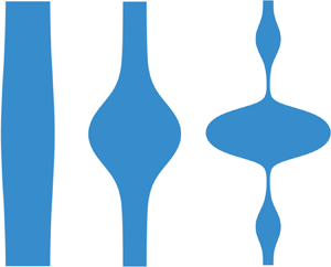
  $\varepsilon \alpha \to \infty $, the breakup dynamics of the leaky-dielectric jet reverts to the EHD breakup of a perfectly conducting jet. The breakup process from perfectly conducting jets is described in this section to provide a comparison for later computations and understand the pinching mechanisms of leaky-dielectric jets. Figure 2 shows the nonlinear evolution of the perfectly conducting and leaky-dielectric jets. For the perfectly conducting jet, as depicted in figure 2(a), the jet peak expands in the radial direction. In contrast, the jet trough is first compressed and then stretched. Eventually, the peak and trough are atomized into the so-called main drop and satellite droplet, which are connected by a thin ligament before pinch-off. This case is called the ligament-pinching mode. The ligament-pinching mode usually exists in inviscid or slightly viscous uncharged jets since a satellite droplet appears (Setiawan & Heister Reference Setiawan and Heister1997). However, at
  $\alpha = 1$, the leaky-dielectric jet finally breaks at the jet end, which is called the end-pinching mode in this study. In this case, the peak is also expanding but its extent is smaller than that in the perfectly conducting case, and no satellite droplet occurs. A highly viscous uncharged jet or an uncharged thread in the Stokes flow limit tends to break via end pinching (Collins et al. Reference Collins, Harris and Basaran2007).

Figure 2. Evolution of the surface profiles of (a) perfectly conducting and (b) leaky-dielectric jets. The bottom panels depict the jet shapes at the incipience of pinch-off. Here,  $k = 0.6,\;Oh = 1,\;C{a_E} = 2$ for both jets and
  $\varepsilon = 10,\;\alpha = 1$ for leaky-dielectric jets.
Figure 3 depicts the variations of the jet amplitude  $A(t)$, which is defined as half of the difference between the maximum and the minimum radii. Such treatment can cancel the errors of second-order terms (Ashgriz & Mashayek Reference Ashgriz and Mashayek1995). The curves of both the perfectly conducting and leaky-dielectric jets first exhibit a linear region, followed by a nonlinear region. Besides, the linear region dominates the thinning process most of the time since the nonlinear effect in this region is fairly weak. Similar regions are also found by Collins et al. (Reference Collins, Harris and Basaran2007) and Wang & Papageorgiou (Reference Wang and Papageorgiou2011) for perfectly conducting jets and Ashgriz & Mashayek (Reference Ashgriz and Mashayek1995) for uncharged jets. In the linear region, the growth rate, viz., the slope of the curve, remains constant. The growth rate in the leaky-dielectric case is lower than that in the perfectly conducting case, and the leaky-dielectric jet breaks earlier than the perfectly conducting case. In the early stage of the linear region, the leaky-dielectric and perfectly conducting jets evolve similarly, e.g. the jet profiles of the two jets at
  $t = 20$ are nearly the same. As the evolution of the jets approach pinch-off, the nonlinear dynamics becomes significant, and the two jets exhibit different behaviour, i.e. ligament pinching in the perfectly conducting case and end pinching in the leaky-dielectric case.

Figure 3. Variation in the jet amplitude at  $z = 0$. Here,
  $k = 0.6,\;Oh = 1,\;C{a_E} = 2,\;\varepsilon = 10,\;\alpha = 1$. The solid lines represent the fitting curves.
Collins et al. (Reference Collins, Harris and Basaran2007) demonstrated that electric stress causes the satellite droplets of perfectly conducting jets to be larger than those of the uncharged cases, even though a highly viscous jet can cause the formation of large satellite drops. However, the charge relaxation suppresses the formation of satellite drops in leaky-dielectric jets. The differences in the charge relaxation effects on the linear and nonlinear dynamics will be comprehensively addressed in the next section.
4. Results and discussion
4.1. Comparison with the linear theory
The framework of the linear theory assumes that the perturbed interface is defined by a complex eigenvalue ![]() and a wavenumber k, i.e.
and a wavenumber k, i.e. ![]() , where
, where  ${\omega _r}$ is the growth rate,
  ${\omega _i}$ is the oscillation frequency and
  $\hat{h} \ll 1$ denotes an infinitesimal amplitude surface disturbance. In this manner, all other quantities, such as the velocity vector, pressure and electrical potential, are represented as
 ![]() , where
, where  ${X_0}$ is the unperturbed value. Substituting these perturbed quantities into the governing equations and boundary conditions, the dispersion relation relating the growth rate to the wavenumber is derived, which reads (López-Herrera et al. Reference López-Herrera, Riesco-Chueca and Gañán-Calvo2005)
 \begin{equation}{\omega ^2}f(k) + {T_\mu } + ({T_\gamma } + {T_E})(1 - {T_{e1}}) + {T_{e2}} + {T_{e3}} = 0,\end{equation}
where
 \begin{equation}{T_\mu } = 2Oh\omega [2{k^2}f(k) - 1] + 4{k^2}O{h^2}({k^2}f(k) - {l^2}f(l))\end{equation}
is the viscous driving term,
 \begin{equation}{T_\gamma } = {k^2} - 1\end{equation}
denotes the surface tension term and
 \begin{equation}{T_E} = C{a_E}\left( {1 + \frac{1}{{G(k)}}} \right)\end{equation}
stands for the electric stress term. Here,  ${T_{e1}}$,
  ${T_{e2}}$ and
  ${T_{e3}}$ are the electric relaxation terms, which are respectively given by
 \begin{equation}\left.
\begin{array}{c@{}} {{T_{e1}} =
\dfrac{{C{a_E}G(k){k^2}f(k)}}{{E(\alpha ,\varepsilon
,\omega ,k){\omega^2}}}({k^2}f(k) - {l^2}f(l)),}\\
{{T_{e2}} = \dfrac{{C{a_E}}}{{E(\alpha ,\varepsilon ,\omega
,k)}}f(k)\left( {2{k^2}f(k) + {k^2}f(k){l^2}f(l)G(k) +
\dfrac{1}{{G(k)}}} \right),} \end{array}\right\}\end{equation}
\begin{equation}\left.
\begin{array}{c@{}} {{T_{e1}} =
\dfrac{{C{a_E}G(k){k^2}f(k)}}{{E(\alpha ,\varepsilon
,\omega ,k){\omega^2}}}({k^2}f(k) - {l^2}f(l)),}\\
{{T_{e2}} = \dfrac{{C{a_E}}}{{E(\alpha ,\varepsilon ,\omega
,k)}}f(k)\left( {2{k^2}f(k) + {k^2}f(k){l^2}f(l)G(k) +
\dfrac{1}{{G(k)}}} \right),} \end{array}\right\}\end{equation}
and
 \begin{equation}{T_{e3}} = \frac{{2C{a_E}Ohf(k){k^2}}}{{E(\alpha ,\varepsilon ,\omega ,k)\omega }}(2 + G(k))({k^2}f(k) - {l^2}f(l)).\end{equation}
Here,  $f(k)$,
  $E(\alpha ,\varepsilon ,\omega ,k)$ and
  $G(k)$ denote the auxiliary functions that are respectively written as
 \begin{equation}f(k) = \frac{{{I_0}(k)}}{{k{I_1}(k)}},E(\alpha ,\varepsilon ,\omega ,k) = \varepsilon \left( {1 + \frac{\alpha }{\omega }} \right)G(k) - f(k),\end{equation}
and
 \begin{equation}G(k) = \frac{{{I_0}(k){K_0}(k{R_0}) - {K_0}(k){I_0}(k{R_0})}}{{k({I_1}(k){K_0}(k{R_0}) + {K_1}(k){I_0}(k{R_0}))}},\end{equation}
where  ${I_n}$ and
  ${K_n}$ are the first- and second-kind modified Bessel functions with the order n and
  ${l^2} = {k^2} + \omega /Oh$. We also deduce the dispersion relation for non-axisymmetric perturbations (see Appendix D). The following sections only focus on the effects of axisymmetric perturbations. When
  $\alpha \varepsilon \to \infty $, the dispersion relation for the perfectly conducting jet is recovered (Collins et al. Reference Collins, Harris and Basaran2007). Figure 4 shows the dispersion relation for the perfectly conducting and leaky-dielectric jets. The growth rates of FEM simulations calculated from the slopes of figure 3 agree well with the linear theory. In the linear stability analysis, several characteristics, including the range of unstable wavenumbers and the maximum growth rate, are usually considered. Since the behaviour at small k is complicated (López-Herrera et al. Reference López-Herrera, Riesco-Chueca and Gañán-Calvo2005), we limit the computed space of wavenumber to
  $[0.2,2]$. A large growth rate indicates the jet is more unstable. In all cases, the leaky-dielectric jet is more stable than the perfectly conducting one at long wavelength
  $(k < 1)$, whereas the instability is nearly the same for the two jets in the short-wave range
  $(k > 1)$. Figure 4(a) depicts the effects of the viscosity
  $Oh$ on the jet instability. In (4.1), the viscosity mainly affects the viscous driving term
  ${T_\mu }$ and the electric relaxation term
  ${T_{e3}}$. Owing to the contribution of
  ${T_\mu }$, the jet is more stable at a large viscosity. Take
  $k = 0.6$ for example, the growth rates for leaky-dielectric cases at
  $Oh = 0.01$,
  $Oh = 0.1$ and
  $Oh = 1$ are 0.0911, 0.2602 and 0.3222, respectively. For perfectly conducting cases, they are 0.0999, 0.2871 and 0.3330, respectively. A similar trend is common in uncharged (Eggers & Villermaux Reference Eggers and Villermaux2008) and perfectly conducting jets (Collins et al. Reference Collins, Harris and Basaran2007). Additionally, the viscosity partly decreases the influence of the charge relaxation due to
  ${T_{e3}}$. However, the range of unstable wavenumbers is unaffected by the viscosity, as well as the relaxation parameter
  $\alpha $ (figure 4c) and permittivity
  $\varepsilon $ (figure 4d). In contrast, the electric field intensity
  $C{a_E}$ dramatically increases the range of unstable wavenumbers, which is
  $0 < k < 1$ for the uncharged jet
  $(C{a_E} = 0)$. In the leaky-dielectric cases, the upper limit of the unstable wavenumber rises to 1.13 for
  $C{a_E} = 0.5$, 1.33 for
  $C{a_E} = 1$ and 1.95 for
  $C{a_E} = 2$, as shown in figure 4(b). This result is mainly caused by an increase in the effects of the electric stress terms
  ${T_E}$. However, the electric relaxation terms
  ${T_{e1}}$,
  ${T_{e2}}$ and
  ${T_{e3}}$ do not influence the upper limit since they approach zero at
 ![]() . Besides, as
. Besides, as  $C{a_E}$ increases, the electric stress firstly decreases the maximum growth rate and then increases it. For the cases at
  $C{a_E} = 0.5$,
  $C{a_E} = 1$ and
  $C{a_E} = 2$, the maximum growth rates for leaky-dielectric jets are 0.0973, 0.09422 and 0.1356, respectively. The change of the unstable wavenumber and maximum growth rate still holds for inviscid (Setiawan & Heister Reference Setiawan and Heister1997) or viscous (Collins et al. Reference Collins, Harris and Basaran2007) perfectly conducting jets. Furthermore, as
  $C{a_E}$ rises, the charged jet becomes more stable above a critical wavenumber but more unstable below this critical value (
 ${k_E}$ for the perfectly conducting jet and
  ${k^{\prime}_E}$ for the leaky-dielectric jet). The theoretical critical value for the perfectly conducting jet is
  ${k_E} = {\varGamma ^{ - 1}}( - 1) = 0.595$ when the electrode radius
  ${R_0}$ tends to infinity (López-Herrera et al. Reference López-Herrera, Riesco-Chueca and Gañán-Calvo2005; Setiawan & Heister Reference Setiawan and Heister1997). In the leaky-dielectric case, the critical value
  ${k^{\prime}_E}$ shifts towards the short wave but is still located on the curve of the dispersion relation of the uncharged jet. Figures 4(c) and 4(d) highlight the influence of charge relaxation on jet stability. Due to the electric relaxation terms
  ${T_{e1}}$,
  ${T_{e2}}$ and
  ${T_{e3}}$, the charge relaxation is sensitive to
  $\alpha $ and
  $\varepsilon $ in the long-wavelength range
  $(k < 1)$ but does not affect the stability in the short-wavelength range
  $(k > 1)$.

Figure 4. Wavenumber dependence on the growth rates obtained from linear analysis (lines) and FEM simulations (symbols). Panels (a–d) represent the effects of viscosity, electric field intensity, relaxation parameter and permittivity on jet stabilities. The solid blue and dashed black lines stand for the leaky-dielectric and perfectly conducting cases, respectively. For the FEM simulations, only the cases at  $k = 0.6$ and
  $k = 0.8$ are displayed. All the results are calculated based on parameters
  $Oh = 1,\;C{a_E} = 2,\;\alpha = 10,\;\varepsilon = 10$.
If the leaky-dielectric jet evolves according to linear theory, it eventually breaks at the time  ${t_b} ={-} \ln ({A_0})/{\omega _r}$. This expression is often used to estimate the breakup time of uncharged (Eggers Reference Eggers1997; Eggers & Villermaux Reference Eggers and Villermaux2008) and perfectly conducting jets (Collins et al. Reference Collins, Harris and Basaran2007). Figure 5 depicts the relationship between the breakup time and the growth rate obtained from linear theory and the FEM simulations. The breakup times at a high relaxation parameter or permittivity obtained from the FEM simulations agree with those derived from linear theory; however, there are deviations from the theoretical values at low
  $\alpha $ and
  $\varepsilon $ (20 % error). This result is caused by the strong nonlinear dynamics in the later evolution of the jet pinching (the nonlinear region in figure 3).

Figure 5. Breakup time as a function of the growth rate obtained from the linear theory (line) and FEM simulations (symbols). For the FEM simulations, only the cases at  $k = 0.6$ and
  $k = 0.8$ are shown.
4.2. Nonlinear breakup of leaky-dielectric jets
To identify the differences of nonlinear dynamics between the perfectly conducting and leaky-dielectric jets, a relative deformation parameter S measuring the deviation of the jet profiles between the two jets is defined as
 \begin{equation}S = \sqrt {\int_0^\lambda {{{({r_{LD}} - {r_{PC}})}^2}\,\textrm{d}z} } ,\end{equation}
where  ${r_{LD}}$ and
  ${r_{PC}}$ denote the surface profiles of the leaky-dielectric and perfectly conducting jets at pinch-off, respectively. Besides, the relative volumes of satellite droplets from leaky-dielectric jets given as
 \begin{equation}V = \frac{{\mathop \smallint \nolimits_{z_{min}^ + }^{\pi /k} r_{LD}^2\,\textrm{d}z}}{{\mathop \smallint \nolimits_0^{\pi /k} r_{LD}^2\,\textrm{d}z}},\end{equation}
are calculated, where  $z_{min}^ + $ is the axial coordinate of the pinch-off point in the domain of
  $z > 0$. Figures 6(a) and 6(b) show the final surface shapes, the relative deformation parameters and the relative satellite volumes at different
  $\alpha $. For the leaky-dielectric jet, the surface profile at
  $\alpha = 10$ nearly overlaps with that of the perfectly conducting case. This result indicates that even at
  $\alpha = 10$, the leaky-dielectric jet can be treated as a pure conductor. Such consideration is also verified by the linear theory, as depicted in figure 4(c). As
  $\alpha $ decreases, a significant effect of the charge relaxation results in the formation of round proto-main drops. Besides, the proto-satellite drops are compressed until no more satellite droplets appear. In the regimes where
  $\alpha > 1.9$ and
  $\alpha < 1.89$, the leaky-dielectric jet is broken via ligament- and end-pinching modes, respectively. Furthermore, a transition regime covering a narrow range of
  $\alpha $ (grey shading in figure 6b) shows that the jet ligament and end are simultaneously compressed. As a result, the proto-satellite droplet slowly merges with the proto-main drop. The satellite volume gets smaller as
  $\alpha $ decreases. If
  $\alpha $ is 1.893, the leaky-dielectric jet may break at the ligament and end simultaneously.

Figure 6. (a) Surface profiles of the leaky-dielectric jets before breakup and (b) relative deformation S (marker) and relative satellite volume V (line) for different relaxation parameters  $\alpha $. Here,
  $k = 0.6,\;Oh = 1, \;C{a_E} = 2,\;\varepsilon = 10$. In (a) at
  $\alpha = 10$, the dashed black profile represents the interface shape of a perfectly conducting jet at pinch-off.
A similar trend is also found at different values of  $\varepsilon $, as depicted in figure 7. As the permittivity increases, the leaky-dielectric jet eventually goes through the end-, transition- and ligament-pinching modes. The three modes are divided by two critical permittivities, viz.,
  $\varepsilon = 17.45$ and
  $\varepsilon = 17.5$. A jet with a high permittivity (
 $\varepsilon = 100$ in figure 7a) shares similar characteristics as a jet at a high relaxation parameter (
 $\alpha = 10$ in figure 6a). Wang (Reference Wang2012) and Li et al. (Reference Li, Ke, Yin and Yin2019) also showed that
  $\alpha $ and
  $\varepsilon $ had the same effect on the nonlinear dynamics of a leaky-dielectric jet. In practical experiments,
  $\alpha $ and
  $\varepsilon $ are interrelated since a highly conducting liquid also exhibits high polarizability. Some weak polar liquids such as canola oil (Collins et al. Reference Collins, Jones, Harris and Basaran2008) and polymers (Ha & Yang Reference Ha and Yang2000) are often employed in investigating the dynamics of leaky-dielectric liquids. Clearly, a decrease in
  $\alpha \varepsilon $ can compress the satellite droplets until no more satellite droplets are formed. Li et al. (Reference Li, Ke, Yin and Yin2019) investigated a moderately viscous, charged, viscoelastic jet, and concluded that the finite conductivity removes satellite droplets from the beads-on-string structure. Nevertheless, in most cases analysed by Li et al. (Reference Li, Ke, Yin and Yin2019), the main drop is slightly affected by the charge relaxation, and the reduction in the satellite droplet size is under the common influences of charge relaxation and viscoelasticity. In this work, we infer that the charge relaxation can suppress the radial enlargement of the satellite droplets from a leaky-dielectric jet.

Figure 7. (a) Surface profiles of the leaky-dielectric jets before breakup and (b) relative deformation S (marker) and relative satellite volume V (line) at different electrical permittivity  $\varepsilon $. Here,
  $k = 0.6,\;Oh = 1,\;C{a_E} = 2, \;\alpha = 1$. In (a), the dashed black profile represents the interface shape of a perfectly conducting jet at pinch-off.
4.3. Experimental verification
A system of electrified jets is developed for observing the pinching process, as shown in figure 8(a). The system primarily contains a jet generating module and a visual observation module. In the jet generating module, as depicted in figure 8(b), a jet is generated from a metal needle which is driven by an injection pump, and then goes through a coaxial electrode. The geometry parameters of the needle–cylinder electrode are listed in table 1. The needle is imposed by a DC high voltage and the electrode is grounded. The drops from broken jets are received by a reservoir. A high-speed camera (Photron SA5) is used to capture the pinching process by using a 2 × 10⁴ f.p.s. frame rate. Pure ethanol is tested in experiments, of which physical properties are listed in table 1. Three groups of operating parameters in experiments are mainly conducted as listed in table 2. In FEM simulations, the Ohnesorge number and charge relaxation parameter are  $Oh = 0.026$ and
  $\alpha = 0.13$, respectively. To repeat the experimental configuration in FEM simulations, gravity is also included by adding a volume force term
  ${F_g}{\boldsymbol{e}_z}$ to the right-hand side of (2.2), where
  ${\boldsymbol{e}_z}$ is the axial unit vector. Based on the dimensionless processing,
  ${F_g}$ is scaled into the Bond number
  $Bo = \bar{\rho }\bar{r}_0^2\bar{g}/\bar{\gamma } \approx 0.0035$ comparing the importance of gravity with surface tension, where
  $\bar{g}$ is the gravitational acceleration. A velocity inlet and an outlet of fully developed flow are imposed on the left and right boundaries of figure 1. Similar boundary conditions were first adopted by Eggers & Dupont (Reference Eggers and Dupont1994) in one-dimensional simulations of uncharged jets. In the dimensionless representation, the inlet velocity is reduced to the Weber number
  $We = \bar{\rho }\bar{U}_0^2{\bar{r}_0}/\bar{\gamma }$, which is the ratio of the inertia force to the surface tension. Besides, the length of the computational domain along the z-axis is set to
  ${\bar{Z}_0} = 8\bar{\lambda }$. In FEM simulations the electrode radius is set to
  ${R_0} = 10$, which is different from the experimental setting
  ${R_0} = 47$; however, the electric capillary numbers in simulations and experiments are kept the same.

Figure 8. (a) Schematic diagram of the experimental apparatus, and (b) the needle–cylinder electrode configuration used in the experiments.
Table 1. Physical properties of ethanol and geometry parameters used in experiments.
Table 2. Operating parameters in experiments.

Figure 9 depicts the snapshot of electrified jets at pinch-off in experiments and FEM simulations; breakage occurs via the ligament-pinching mode. In FEM simulations,  $We$,
$We$,  $C{a_E}$ and k are adjusted to model the experiment as accurately as possible. The profiles of leaky-dielectric jets are close to these in experiments. Figure 9(a) shows the surface profiles of the leaky-dielectric and perfectly conducting jets before the breakup. In the presence of the electric field, the main drops in the experiment (A and C) and in the FEM simulation (A, C, A'‘ and C'‘) are stretched in the radial direction. Moreover, the main drop is more oblate in the downstream area (A, A’ and A'‘) than in the upstream area (C, C’ and C'‘). This result is caused by strong normal electric stresses. However, the main and satellite drops are more compressed in the leaky-dielectric jet than in the perfectly conducting jet. As a result, the sizes of satellite droplets from leaky-dielectric jets are smaller than their counterparts formed from perfectly conducting jets at the same
  $Oh$ and
  $C{a_E}$. Collins et al. (Reference Collins, Harris and Basaran2007) showed a ring-like structure (A'‘) appeared to be forming at the periphery of the main drop at very high
  $C{a_E}$ (
 $> 6.5 \times 2/{(\ln 10)^2} = 2.45$). In contrast, the leaky-dielectric jet tends to form oblate drops before breakup at the same conditions.

Figure 9. Comparisons between experiments and FEM simulations. (a)  $We = 12,\;C{a_E} = 2.5,\;k = 0.95$, (b)
  $We = 8.5,\;C{a_E} = 2.5,\;k = 0.92$ and (c)
  $We = 12,\;C{a_E} = 2.3,\;k = 0.9$. Here, LD and PC represent the leaky-dielectric and perfectly conducting jets, respectively.
4.4. Charge relaxation and stress jump at the interface
From (2.8), it is known that a large conductivity  $\alpha \varepsilon $ indicates a strong ohmic conduction in the charge transportation. Conversely, a low conductivity
  $\alpha \varepsilon $ causes a strong surface convection. Figure 10 depicts the fluid flow inside the liquid domain and the distributions of the surface velocities. For a leaky-dielectric jet with a large conductivity
  $(\alpha \varepsilon = 100)$, the fluid flows from the jet ligament to the proto-main drop and proto-satellite droplet, which is similar to the results of Collins et al. (Reference Collins, Harris and Basaran2007) in the perfectly conducting case. However, for a leaky-dielectric jet with moderate conductivity
  $(\alpha \varepsilon = 18.9)$, the fluid flows not only from the jet ligament to the main and satellite drops but also from the jet end to the proto-satellite droplet. The flow direction can be distinguished by a flow stagnation plane (marked by the black line in figure 10a). On the flow stagnation plane, the axial velocity is zero, as shown in figure 10(b). When the right half-side of the streamlines is
  $\alpha \varepsilon = 100$, the surface convection comes into effect because the surface charge is convected along the streamlines. This causes the surface charge to accumulate at the surface of the proto-main and proto-satellite drops. However, on the other hand, the ohmic conduction drives the charge moving into the ligament. As
  $\alpha \varepsilon $ decreases, the surface charge convection becomes increasingly important so that the main and satellite drops carry more charges. The accumulated charges affect the electric field and, in turn, modify the distribution of surface charges. Meanwhile, the transported charges also influence fluid flow. In figure 10(b), the position at the maximum radial velocity indicates the plane of the minimum radius or the pinch-off position. Hence, for the jet at
  $\alpha \varepsilon = 100$ and
  $\alpha \varepsilon = 10$, only the ligament and end are pinched, respectively, while for the jet at
  $\alpha \varepsilon = 18.93$, the ligament and end are simultaneously pinched.

Figure 10. (a) Streamlines and (b) surface velocities of leaky-dielectric jets at  $Oh = 1,\;C{a_E} = 2$ and
  $k = 0.6$. The red and black lines in (a) indicate the locations of the minimum radius and the interior stagnation plane, respectively.
Considering the distribution of surface charges at the jet end  $z = \pi /0.6$, in the early stage of charging, the surface charge density can be evaluated by the linear theory. Hence, the charge densities for the three cases increase exponentially. As time progresses, the surface charge density still rises exponentially but with a smaller exponent. When the jet approaches pinch-off, the surface charge density at
  $\varepsilon \alpha = 100$ increases gently, whereas those at
  $\varepsilon \alpha = 10$ and
  $\varepsilon \alpha = 18.93$ rise exponentially again. In the initial stage of jet pinching, the contribution of the surface charge convection is much less than that of the ohmic conduction; thus, the leaky-dielectric jets behave as perfect conductors in all cases. With the increase in the jet deformation, the increasing fluid flow drives the surface charge convection, which becomes comparable to the ohmic conduction. For a leaky-dielectric jet at a low value of
  $\varepsilon \alpha = 18.93$, the surface charge density first rapidly accumulates and then increases with a moderate growth rate, and ultimately rises dramatically again, as shown in the regions A, B and C in figure 11(a). The monotonic growth of the surface charge density also occurs in the end-pinching or conical end breakup of electrified drops (Sengupta et al. Reference Sengupta, Walker and Khair2017). The result of the surface charge density before breakup due to the ohmic conduction and surface charge convection is depicted in figure 11(b). For the jet at
  $\varepsilon \alpha = 100$, most of the surface charge is accumulated at position
  $z \approx{\pm} 2$, i.e. the ligament. In contrast, the charge is concentrated around the jet end for
  $\varepsilon \alpha = 10$. The jet at
  $\varepsilon \alpha = 18.93$ is the combination of the former two cases, in which most charges are accumulated at the jet end and ligament. Figure 11(c) shows the strength of the ohmic conduction term
  $\varepsilon \alpha {\boldsymbol{E}_L}\boldsymbol{\boldsymbol{\cdot} }\boldsymbol{n}$ and the surface charge convection term
  $- {\nabla _s}\boldsymbol{\boldsymbol{\cdot} }(q\boldsymbol{u})$ when the jet approaches pinch-off. At
  $\varepsilon \alpha = 100$, the strength of ohmic conduction at the pinch-off point is larger than the surface convection one. As
  $\varepsilon \alpha $ is reduced to 10, the significance of the surface charge convection at the breakup point exceeds the conduction. However, for the jet at
  $\varepsilon \alpha = 18.93$, the roles of the convection and conduction at the jet end or ligament are of equal importance.

Figure 11. (a) Evolution of the surface charge density at  $z = \pi /0.6$, (b) the distribution of the surface charge density before breakup and (c) the importance of ohmic conduction and surface charge convection terms before breakup. Here,
  $Oh = 1,\;C{a_E} = 2,\;k = 0.6$. For (c), the conduction and convection terms are plotted in the regions of
  $z < 0$ and
  $z > 0$, respectively.
Stress analyses are used to expound on the pinching mode. Equation (2.5) is rewritten in the form of normal and tangential components
 \begin{equation}\left.
{\begin{array}{c@{}} {p -
\boldsymbol{n}\boldsymbol{\boldsymbol{\cdot} }{{\mathbb T}}_L^\mu
\boldsymbol{\boldsymbol{\cdot} }\boldsymbol{n} = {p_C} + {p_{E,n}},}\\
{\boldsymbol{n}\boldsymbol{\boldsymbol{\cdot}
}{{\mathbb T}}_L^\mu \boldsymbol{\boldsymbol{\cdot}
}\boldsymbol{\tau } = {p_{E,\tau }},} \end{array}}
\right\}\end{equation}
\begin{equation}\left.
{\begin{array}{c@{}} {p -
\boldsymbol{n}\boldsymbol{\boldsymbol{\cdot} }{{\mathbb T}}_L^\mu
\boldsymbol{\boldsymbol{\cdot} }\boldsymbol{n} = {p_C} + {p_{E,n}},}\\
{\boldsymbol{n}\boldsymbol{\boldsymbol{\cdot}
}{{\mathbb T}}_L^\mu \boldsymbol{\boldsymbol{\cdot}
}\boldsymbol{\tau } = {p_{E,\tau }},} \end{array}}
\right\}\end{equation}
where  ${{\mathbb T}}_L^\mu = Oh(\boldsymbol{\nabla }\boldsymbol{u} + {(\boldsymbol{\nabla }\boldsymbol{u})^\textrm{T}})$ is the viscous stress inside the liquid domain,
  ${p_C} = \kappa $ denotes the capillary pressure,
  ${p_{E,n}} ={-} C{a_E}[(E_{G,n}^2 - \varepsilon E_{L,n}^2) - (1 - \varepsilon )E_\tau ^2]/2$ and
  ${p_{E,\tau }} ={-} C{a_E}q{E_\tau }$ are the electric stress jumps of the normal and tangential components, respectively. The normal electric stress jump provides the jet interface with an inward driving force while the surface tension causes rounding of the surface. For a perfectly conducting liquid, the normal and the tangential electric stresses across the interface can be simplified to
  ${p_{E,n}} ={-} C{a_E}{q^2}/2$ and
  ${p_{E,\tau }} = 0$, respectively. The more surface charges accumulate, the larger the normal electrical stress is. Figure 12 shows the normal stress jump and tangential stress across the interface. For the pressures of stress in the cases of
  $\varepsilon \alpha = 100$ and
  $\varepsilon \alpha = 18.93$, the capillary pressure (absolute value) at
  $z \approx{\pm} 2$ is larger than the normal electric stress, as marked by the red arrows in figures 12(a) and 12(c). Hence, the two cases eventually break at the ligament. In contrast, at
  $\varepsilon \alpha = 18.93$ and
  $\varepsilon \alpha = 10$, a large normal electric stress due to the accumulated charges causes the jets to break at the jet end, as marked by the green arrows in figures 12(c) and 12(e). In figures 12(b), 12(d) and 12(f), the effect of the tangential electric stress is more significant as
  $\alpha $ decreases. For the three cases, the maximum normal electric stresses are approximately
  $\alpha $ to
  ${\alpha ^2}$ times the maximum tangential ones. The tangential electric stress increases the interface flow, resulting in streamlines as depicted in figure 10(a).

Figure 12. Normal stress jump and tangential stress for leaky-dielectric jets at (a,b)  $\varepsilon \alpha = 100$, (c,d)
  $\varepsilon \alpha = 18.93$ and (e,f)
  $\varepsilon \alpha = 10$. In the left panels, the solid black and dashed blue lines represent the normal electric stress jump
  ${p_{E,n}}$ and capillary pressure
  ${p_C}$, respectively. Here,
  $Oh = 1,\;C{a_E} = 2,\;k = 0.6$.
4.5. Effects of the wavenumber, electric field intensity and viscosity on the pinch-off
Figure 13 highlights the effects of the wavenumber k, electric field intensity  $C{a_E}$ and viscosity
  $Oh$ on the pinch-off. Ashgriz & Mashayek (Reference Ashgriz and Mashayek1995) demonstrated that the size of the satellite drops in uncharged cases decreases with an increase in the wavenumber. Besides, the satellite drop size declines as the viscosity increases. Collins et al. (Reference Collins, Harris and Basaran2007) showed that large electric stresses significantly increase the radii of the satellite drops in viscous, pure conducting jets. These trends also hold for leaky-dielectric jets. As shown in figure 13(a), as the wavenumber increases, the leaky-dielectric jet first goes through the ligament-pinching mode and then the end-pinching mode. A comparison with the perfectly conducting cases indicates that a high wavenumber hinders the formation of satellite droplets in the leaky-dielectric cases. At
  $k = 0.6$ and
  $k = 0.7$, the leaky-dielectric jets break via the ligament-pinching mode, whereas they break via the end-pinching mode at
  $k = 0.8$. In figure 13(b), the leaky-dielectric jet breaks via the end-pinching mode at a low electric field intensity and the ligament-pinching mode at a high electric field intensity. If a jet is a perfect conductor, a low electric field intensity of
  $C{a_E} = 0.5$ can slightly increase the size of the satellite droplet when comparing with an uncharged jet at
  $Oh = 1$. However, for a leaky-dielectric jet, the charge relaxation prevents the formation of satellite droplets, even though the jet exhibits high but not infinite conductivity. As a result, the jet breaks via the end-pinching mode at
  $C{a_E} = 0.5$. In contrast, the leaky-dielectric jets at
  $C{a_E} = 1$ and
  $C{a_E} = 1.5$ break via the ligament-pinching mode. Figure 13(c) shows that a weak viscosity can enhance the effect of the charge relaxation; thus, the jet end is substantially compressed at
  $Oh = 0.01$. It is noticed that the transition-pinching mode does not show in figure 13 because it occurs within a narrow range of
  $\varepsilon \alpha $. Under the conditions of figure 13(a–c), the transition-pinching mode should occur at a wavenumber of
  $0.7 < k < 0.9$, an electric field intensity of
  $0.5 < C{a_E} < 1$ and a viscosity of
  $Oh < 0.01$, respectively.

Figure 13. Influence of the wavenumber k, viscosity  $Oh$ and electric field intensity
  $C{a_E}$ on the pinch-off. For (a),
  $Oh = 1,\;C{a_E} = 2,\;\varepsilon \alpha = 20$. For (b)
  $Oh = 1,\;k = 0.6,\;\varepsilon \alpha = 1000$. For (c),
  $C{a_E} = 2,\;k = 0.6, \varepsilon \alpha = 100$. The dashed black and solid blue profiles represent the interface shapes of the perfectly conducting and leaky-dielectric jets at pinch-off, respectively.
Figure 14 depicts the breakup mode in the  $k - C{a_E}$ space. The computed space is
  $[0.4,1.2] \times [0.5,2]$. At a small
  $\varepsilon \alpha = 20$, the leaky-dielectric jet breaks via the ligament-pinching mode only at a large electric field intensity
  $(C{a_E} = 2)$ and a long-wavelength range
  $(0.4 < k < 0.7)$. As
  $\varepsilon \alpha $ increases, the boundary of the ligament-pinching mode expands so that the leaky-dielectric jet can break at small electric field intensities and a short-wavelength range. If
  $\varepsilon \alpha $ tends to infinity, the perfectly conducting limit is recovered, and the jet only breaks via the ligament-pinching mode.

Figure 14. Breakup modes of viscous  $(Oh = 1)$, charged jets in the
  $k - C{a_E}$ plane. The symbols indicate the calculated data points. The closed line represents the boundary of the ligament-pinching mode.
4.6. Local dynamics at pinch-off
When a jet approaches pinch-off, a singularity forms since one piece of fluid is separated into two discontinuous ones. Following Eggers’ dimensional analysis (Eggers & Fontelos Reference Eggers and Fontelos2015), the profile of a charged jet close to pinch-off is represented by
 \begin{equation}\bar{h} = \bar{f}({\rm \Delta}\bar{z},{\rm \Delta}\bar{t},\bar{\rho },\bar{\mu },\bar{\gamma },\bar{g},\bar{\varepsilon },{\bar{E}_0},\bar{K},{\bar{r}_0}),\end{equation}
where  ${\rm \Delta}\bar{z} = \bar{z} - {\bar{z}_0} \to 0$ and
  $\Delta \bar{t} = {\bar{t}_b} - \bar{t} \to 0$ are the scaled space and time coordinates of the breakup point. By using the characteristic length
  ${\bar{l}_t} = \sqrt {\bar{\mu }{\rm \Delta}\bar{t}/\bar{\rho }} $ as the breakup scale, (4.11) can be simplified to
 \begin{equation}\bar{h} = {\bar{l}_t}\,f\left( {\frac{{{\rm \Delta}\bar{z}}}{{{{\bar{l}}_t}}},\frac{{{{\bar{l}}_\mu }}}{{{{\bar{l}}_t}}},\frac{{{{\bar{l}}_\gamma}}}{{{{\bar{l}}_t}}},\frac{{{{\bar{l}}_\textrm{E}}}}{{{{\bar{l}}_t}}},\frac{{{{\bar{l}}_\textrm{e}}}}{{{{\bar{l}}_t}}},\frac{{{{\bar{r}}_0}}}{{{{\bar{l}}_t}}}} \right),\end{equation}
where  ${\bar{l}_\mu } = {\mu ^2}/\rho \gamma $ and
  ${\bar{l}_\gamma} = \sqrt {\bar{\gamma }/(\bar{\rho }\bar{g})} $ are the intrinsic viscous scale and the capillary length, respectively. Here, we introduce two characteristic lengths
  ${\bar{l}_E} = \bar{\gamma }/({\bar{\varepsilon }_0}\bar{E}_0^2)$ and
  ${\bar{l}_e} = {\alpha ^2}\bar{\gamma }/({\bar{\varepsilon }_0}\bar{E}_0^2)$ to characterize the effects of the normal and tangential electric stresses. The normal electric stress is assumed to be
  ${\alpha ^2}$-fold the tangential electric stress. These scales can be rewritten as
  ${\bar{l}_\mu } = \sqrt {Oh} {\bar{r}_0}$,
  ${\bar{l}_\gamma } = {\bar{r}_0}Bo$,
  ${\bar{l}_E} = {\bar{r}_0}/C{a_E}$ and
  ${\bar{l}_e} = {\alpha ^2}{\bar{r}_0}/C{a_E}$. In the limit
  ${\bar{l}_t} \to 0$, the macroscopic scales, including
  ${\bar{l}_\gamma }$ and
  ${\bar{r}_0}$ should be ignored due to
  ${\bar{l}_\gamma }/{\bar{l}_t} \to \infty $ and
  ${\bar{r}_0}/{\bar{l}_t} \to \infty $. Hence, (4.12) is reduced to
 \begin{equation}\bar{h} = {\bar{l}_t}\,f\left( {\frac{{\Delta \bar{z}}}{{{{\bar{l}}_t}}},\frac{{{{\bar{l}}_\mu }}}{{{{\bar{l}}_t}}},\frac{{{{\bar{l}}_E}}}{{{{\bar{l}}_t}}},\frac{{{{\bar{l}}_e}}}{{{{\bar{l}}_t}}}} \right).\end{equation}
If  ${\bar{l}_e} \gg {\bar{l}_\mu }$, viz.,
  $C{a_E} \ll {\alpha ^2}/\sqrt {Oh} $,
  ${\bar{l}_e}$ can be dropped out and then (4.13) is left with
 \begin{equation}\bar{h} = {\bar{l}_t}\,f\left( {\frac{{\Delta \bar{z}}}{{{{\bar{l}}_t}}},\frac{{{{\bar{l}}_\mu }}}{{{{\bar{l}}_t}}},\frac{{{{\bar{l}}_E}}}{{{{\bar{l}}_t}}}} \right).\end{equation}
In the same manner, as $\; C{a_E} \ll 1/\sqrt {Oh} $,
  ${\bar{l}_E}$ should be neglected so that the above equation is recovered to
 \begin{equation}\bar{h} = {\bar{l}_t}\,f\left( {\frac{{\Delta \bar{z}}}{{{{\bar{l}}_t}}},\frac{{{{\bar{l}}_\mu }}}{{{{\bar{l}}_t}}}} \right),\end{equation}
which indicates that the electrified jet obeys the scaling laws of uncharged jets. For uncharged jets, the local dynamics can be described by three self-similar regimes, i.e. the inertial (I), viscous (V) (Papageorgiou Reference Papageorgiou1995) and viscous–inertial (VI) regimes (Eggers Reference Eggers1997; Eggers & Villermaux Reference Eggers and Villermaux2008). The dimensionless minimum radius  ${h_{min}}$ of the jet obeys power laws as follows:
 \begin{equation}\left.
{\begin{array}{ll@{}} {{h_{min}} \approx 0.7{{[Oh({t_b}
- t)]}^{2/3}}}&{\textrm{in}\;\textrm{I regime}}\\
{{h_{min}} \approx 0.0709({t_b} -
t)}&{\textrm{in}\;\textrm{V regime}}\\ {{h_{min}} \approx
0.0304({t_b} - t)}&{\textrm{in}\;\textrm{VI regime}}
\end{array}}
\right\}.\end{equation}
\begin{equation}\left.
{\begin{array}{ll@{}} {{h_{min}} \approx 0.7{{[Oh({t_b}
- t)]}^{2/3}}}&{\textrm{in}\;\textrm{I regime}}\\
{{h_{min}} \approx 0.0709({t_b} -
t)}&{\textrm{in}\;\textrm{V regime}}\\ {{h_{min}} \approx
0.0304({t_b} - t)}&{\textrm{in}\;\textrm{VI regime}}
\end{array}}
\right\}.\end{equation}
Collins et al. (Reference Collins, Harris and Basaran2007) showed that the electric field does not affect the pinching dynamics by investigating a perfectly conducting jet at  $Oh = 0.01$ and
  $C{a_E} = 5 \times 2/{(\ln 10)^2} = 1.886$. Our simulations show that the scaling law
  ${h_{min}} \propto {({t_b} - t)^{2/3}}$ holds true for the leaky-dielectric jets at low
  $Oh$ (figure 15a) since
  $C{a_E} \ll {\alpha ^2}/\sqrt {Oh} $ and
  $C{a_E} \ll 1/\sqrt {Oh} $ are satisfied. The phase diagram of breakup regimes (Li & Sprittles Reference Li and Sprittles2016) shows that the 2/3 scaling law for a jet with
  $Oh = 0.01$ is applicable when
  ${h_{min}}$ is smaller than
  $2\sim 4 \times {10^{ - 3}}$. This rule is valid for the leaky-dielectric jet at
  $\varepsilon \alpha = 100$, i.e. a highly conducting jet. In contrast, the scaling law for a leaky-dielectric jet at
  $\varepsilon \alpha = 10$ no longer holds when
  ${h_{min}}$ decreases below
  $2 \times {10^{ - 2}}$. At high values of
  $Oh$, as shown in figure 15(b), the minimum radius near pinch-off point is linear with
  $({t_b} - t)$. The slopes of both the highly
  $(\varepsilon \alpha = 100)$ and weakly conducting jets
  $(\varepsilon \alpha = 10)$ are close to 0.0709; therefore, the V regime adequately describes the pinch-off of viscous, leaky-dielectric jets.

Figure 15. Minimum radii versus time during the breakup of (a) weakly viscous  $(Oh = 0.01)$ and (b) viscous
  $(Oh = 1)$ leaky-dielectric jets. The symbols and solid lines represent the FEM simulations and theoretical curves of uncharged jets, respectively. For (a,b), the electric capillary number is
  $C{a_E} = 2$, and the wavenumber is
  $k = 0.6$.
5. Conclusions
In this work, a two-dimensional axisymmetric model is established to investigate the influence of charge relaxation on the breakup of a leaky-dielectric, Newtonian liquid jet computationally. The charge relaxation was characterized by the relaxation parameter  $\alpha $ and the permittivity of the liquid
  $\varepsilon $. The two dimensionless parameters determine the strength of the charge relaxation, including the ohmic conduction and the surface charge convection. In the early evolution of the leaky-dielectric jet, the linear characteristics, such as the unstable wavenumber and the growth rate, primarily depend on the Ohnesorge number
  $Oh$ and the electric capillary number
  $C{a_E}$. Moreover, they are slightly affected by
  $\alpha $ and
  $\varepsilon $ in the short-wavelength range. In the later development of jet pinching, the breakup modes involving nonlinear dynamics are highly sensitive to
  $\alpha $ and
  $\varepsilon $. At large values of
  $\varepsilon \alpha $, ligament pinching occurs since the strong ohmic conduction supports the charge relaxation from the bulk fluid to the jet surface. In contrast, at small values of
  $\varepsilon \alpha $, strong surface charge convection causes end pinching. Furthermore, a balance between the ohmic conduction and the surface charge convection results in jet breaking via the transition-pinching mode. It has been demonstrated that the capillary pressure is responsible for ligament pinching, whereas the normal electric stress accounts for end pinching. An analysis of the self-similar characteristic at pinch-off indicates that the power law of a leaky-dielectric jet is unaffected by the charge relaxation when
  $C{a_E} \ll {\alpha ^2}/\sqrt {Oh} $ and
  $C{a_E} \ll 1/\sqrt {Oh} $.
Acknowledgements
The authors also thank X. Pan for inspiring discussions.
Funding
This work was supported by the National Key Research and Development Program of China (2018YFA0703203) and the National Natural Science Foundation of China (no. 51876071).
Declaration of interests
The authors report no conflict of interest.
Author contributions
Q.N. performed the simulations, derived the theory and wrote the paper. F.L. carried out the experiment. Q.M. reviewed and edited the paper. H.F. and Z.Y. gave the idea.
Appendix A. Initial perturbations: linear vs. weakly nonlinear
Based on Yuen's (Reference Yuen1968) nonlinear analysis of uncharged jets, the influence of the weakly nonlinear perturbation in the form of  ${S_f} = 1 + {A_0}\cos (kz) - A_0^2/4 - A_0^4/32 + \cdots $ on the pinching of charged jets is examined. As depicted in figure 16, curve fitting shows that the three perturbations share the same slope of 0.0921, which is close to the growth rate of 0.0933 derived from the linear theory. Furthermore, the jet profiles at the incipience of pinch-off exhibit identical shapes. An initial linear perturbation in the form of
  ${S_f} = 1 + {A_0}\cos (kz)$ is appropriate to reproduce the nonlinear dynamics of leaky-dielectric jets.

Figure 16. Variation of the jet amplitude at  $z = 0$. The linear perturbation is in the form of
  ${S_f} = 1 + {A_0}\cos (kz)$, and the nonlinear 1 and 2 are in the forms of
  ${S_f} = 1 + {A_0}\cos (kz) - A_0^2/4$ and
  ${S_f} = 1 + {A_0}\cos (kz) - A_0^2/4 - A_0^4/32$, respectively. Here
  $Oh = 1,\;C{a_E} = 2,\;\varepsilon = 10,\;\alpha = 2,\;k = 0.6,\;{A_0} = 0.01$.
Appendix B. Influence of initial amplitude on pinching
It is known that a linear or nonlinear stability analysis is only valid for small-amplitude perturbations, i.e.  ${A_0} \ll 1$. For the nonlinear simulation of electrified jets, Setiawan & Heister (Reference Setiawan and Heister1997) used
  ${A_0} = 0.001$, whereas Collins et al. (Reference Collins, Harris and Basaran2007) and Wang & Papageorgiou (Reference Wang and Papageorgiou2011) adopted
  ${A_0} = 0.01$. Here, the effect of
  ${A_0}$ on the jet pinching is evaluated. Although the electrified jet is affected by perturbations with different initial amplitudes, the growth rates in the linear region and the maximum amplitude at pinch-off (marked by red line) are the same, as shown in figure 17(a). The breakup time rises linearly with a decrease in the logarithmic initial amplitude, which deviates from the linear relation
  ${t_b} ={-} \ln ({A_0})/{\omega _r}$ at small values of
  ${A_0}$ (figure 17b). However, the initial amplitude does not affect the jet profile at pinch-off. Consequently, it is feasible to set the initial amplitude to
  ${A_0} = 0.01$ to reproduce the nonlinear dynamics of leaky-dielectric jets.

Figure 17. (a) Variation of the jet amplitude at  $z = 0$ and (b) breakup time at different initial amplitudes. Here,
  $Oh = 1,\;C{a_E} = 2,\;\varepsilon = 10,\;\alpha = 2,\;k = 0.6$.
Appendix C. Convergence tests
Figure 18 shows the analyses of spatial and temporal resolutions. The grid partition is depicted in figure 18(a). We test three kinds of grid numbers ( $N = 10$,
  $N = 20$ and
  $N = 30$) and three types of time steps (
 ${\rm \Delta} t = 0.01$,
  ${\rm \Delta} t = 0.001$ and
  ${\rm \Delta} t = \textrm{free}$). Here,
  ${\rm \Delta} t = \textrm{free}$ indicates the time step is computed from the Courant–Friedrichs–Lewy condition. The results show the jet shapes are unaffected by the spatial and temporal resolutions. Moreover, the volume of the jet at different cases is conserved (volume loss:
  $N = 10,1\,{\%}$;
  $N = 20,0.5\,{\%}$;
  $N = 30,0.4\,{\%}$;
  ${\rm \Delta} t = \textrm{free},0.5\,{\%}$;
  ${\rm \Delta} t = \textrm{0}\textrm{.01},0.6\,{\%}$;
  ${\rm \Delta} t = \textrm{0}\textrm{.001},0.5\,{\%}$). In this paper
  $N = 20$ and
  ${\rm \Delta} t = \textrm{free}$ are selected to complete the FEM simulations.

Figure 18. (a) Example of coarse mesh and convergence tests for the amplitude at different (b) grid resolutions and (c) time steps and for the jet volume at different (d) grid resolutions and (e) time steps. Here,  $Oh = 1, \;C{a_E} = 2,\;\varepsilon = 10,\;\alpha = 2,\;k = 0.6$.
Appendix D. Non-axisymmetric perturbations
When all the variables are decomposed as temporal normal modes
where n is the azimuthal wavenumber, the dispersion relation for non-axisymmetric perturbations is given as

with

The above equation is complicated; here, we only discuss the jet instability under the cases of  $n = 1$ and
  $n = 0$. In figure 19(a), the maximum growth rates of non-axisymmetric cases are 0.6884 for
  $Oh = 0.01$, 0.6134 for
  $Oh = 0.1$ and 0.5089 for
  $Oh = 1$. At axisymmetric cases, the growth rates are 0.7335, 0.5567 and 0.1358, respectively. This indicates that the non-axisymmetric motions are more unstable than the axisymmetric ones at high viscosity. In the presence of surface charges (figure 19b), the influences of non-axisymmetric perturbations become significant at large electric capillary numbers. The results agree with Saville's analysis (Saville Reference Saville1971b). In our experiments, a low-viscosity liquid and a large electric field intensity are used. For the experiments at
  $k = 0.9$, the linear theory predicts that the growth rates of non-axisymmetric perturbations are larger than the axisymmetric ones, while the maximum growth rates of the two cases are almost the same. However, our experiments only remain the axisymmetric deformation since the amplitude of non-axisymmetric perturbations is much less than the axisymmetric one. In many experiments (Gañán-Calvo et al. Reference Gañán-Calvo, López-Herrera, Herrada, Ramos and Montanero2018; Sahay, Teo & Chew Reference Sahay, Teo and Chew2013), only the highly viscous liquids, such as polymer solutions, support the non-axisymmetric deformations. For such liquids, the growth rates of non-axisymmetric perturbations are an order of magnitude higher than the axisymmetric ones. Under such cases, the non-axisymmetric motions dominate the jet deformation although their perturbed amplitude is small.

Figure 19. Effect of the (a) viscosity and (b) electric field intensity on the growth rate  ${\omega _r}$ at the axisymmetric
  $(n = 0)$ and non-axisymmetric
  $(n = 1)$ cases. Here, for (a)
  $C{a_E} = 2,\;\varepsilon = 10,\;\alpha = 2$, for (b)
  $Oh = 1,\;\varepsilon = 10, \;\alpha = 2$ and for experiment
  $C{a_E} = 2.5,\;Oh = 0.026,\;\varepsilon = 24.3,\;\alpha = 0.13$.


