


1. Introduction
The flow past a backward-facing step is a canonical amplifier of noise originating from either the inflow boundary or the initial conditions. This noise amplification can be related to flow oscillations, such as vortex shedding (Kaiktsis & Monkewitz Reference Kaiktsis and Monkewitz2003), flapping of separated shear layers (Schäfer, Breuer & Durst Reference Schäfer, Breuer and Durst2009) and three-dimensionality (Barkley, Gomes & Henderson Reference Barkley, Gomes and Henderson2002), and subsequently leads to laminar–turbulence transition or structure fatigue (Mcgregor & White Reference Mcgregor and White1970). The noise amplification can be suppressed by modifying the base flow to be less sensitive to perturbations. The technique of base flow modification is introduced in § 1.1, and the flow past a backward-facing step is reviewed in § 1.2.
1.1. Base flow modifications
Many basic flows, such as boundary layer flow, channel flow, flow past bluff bodies and vortex flow, act as either oscillators or noise amplifiers (Huerre & Monkewitz Reference Huerre and Monkewitz1990). For oscillators that are asymptotically unstable to initial perturbations, it is possible to modify the base flow by a small magnitude so as to change the asymptotic instability characteristics. Investigations of such base flow modifications began with localized studies of incompressible flow, e.g. sensitivity analyses of eigenvalues of the Orr–Sommerfeld operator with respect to modifications of the base flow (Bottaro, Corbett & Luchini Reference Bottaro, Corbett and Luchini2003) and optimal distortion of a base flow with a Hagen–Poiseuille profile to stabilize the most unstable modes of the locally defined linearized Navier–Stokes (NS) operator (Gavarini, Bottaro & Nieuwstadt Reference Gavarini, Bottaro and Nieuwstadt2004). These localized studies of variation of base flow velocity profiles in incompressible flow were extended to variation of velocity and density profiles in compressible flow by Lesshafft & Marquet (Reference Lesshafft and Marquet2010). The global counterpart of the effects of base flow variation on instabilities, i.e. the sensitivity of the most unstable global mode to variation of the base flow, has been investigated in the context of flow past a circular cylinder by Marquet, Sipp & Jacquin (Reference Marquet, Sipp and Jacquin2008b ).
For amplifiers, which are usually asymptotically stable but exhibit strong transient energy growth, base flow variation with respect to the transient energy growth (amplification of the optimal initial perturbation) is more meaningful than with respect to stabilities (amplification of the most unstable mode). Such base flow modifications to minimize or maximize the transient growth of the optimal initial perturbations have been conducted in the context of a flat-plate boundary layer flow, and it was found that a very weak modification of the base flow has a significant impact on amplification of Tollmien–Schlichting (TS) waves (Brandt et al. Reference Brandt, Sipp, Pralits and Marquet2011).
Modification of the base flow can be achieved by a direct modification (Marquet et al. Reference Marquet, Sipp and Jacquin2008b ), by blowing/suction imposed on the boundary (Lashgari et al. Reference Lashgari, Tammisola, Citro, Juniper and Brandt2014), by adding a body force to the governing equations (Brandt et al. Reference Brandt, Sipp, Pralits and Marquet2011) and so forth. The body force can be, among others, a Lorenz force generated by electrodes and magnets mounted in a solid body (Zhang, Fan & Chen Reference Zhang, Fan and Chen2010) or a hydrodynamic force generated by a small cylinder introduced into the domain. This ‘small control cylinder’ exerts a force on the base flow which is opposite to its drag, and has been shown to be effective in suppressing vortex shedding downstream of a cylinder, as experimentally investigated by Strykowski & Sreenivasan (Reference Strykowski and Sreenivasan1990) and numerically studied by Giannetti & Luchini (Reference Giannetti and Luchini2007).
Most of these previous studies on base flow modifications concentrated on the evolution of initial perturbations in the form of either the most unstable modes or the optimal initial perturbations. However, for base flows acting as noise amplifiers, the initial perturbations will be convected out of the domain after a sufficiently long time interval, and therefore the receptivity to temporally continuous inflow/free-stream noise may be more appropriate than initial perturbations for describing the dynamics of this type of base flow. Most existing studies on receptivity to boundary noise have focused on the response of the base flow to prescribed boundary disturbances in the form of free-stream noise or wall roughness and the connection between free-stream noise and instabilities or laminar–turbulence transition (Schrader, Brandt & Henningson Reference Schrader, Brandt and Henningson2009; Zaki et al. Reference Zaki, Wissink, Rodi and Durbin2010). The optimal boundary perturbation, or the most energetic perturbation over a given time horizon, has been calculated in the form of wall-normal disturbances in a locally defined swept Hiemenz flow (Guégan, Schmid & Huerre Reference Guégan, Schmid and Huerre2006) and in a boundary layer flow (Cathalifaud & Luchini Reference Cathalifaud and Luchini2000). These local studies on optimal boundary perturbations have been extended to the global scope to calculate the global optimal inflow perturbation to stenotic flow (Mao, Blackburn & Sherwin Reference Mao, Blackburn and Sherwin2012) and vortex flow (Mao, Blackburn & Sherwin Reference Mao, Blackburn and Sherwin2013).
In the present work, the technique of base flow modification and the concept of global optimal receptivity to boundary perturbations are combined to calculate the variation of a base flow that maximizes or minimizes its optimal receptivity to boundary noise, referring to the maximum gain stemming from the most energized boundary perturbation, rather than the gain of an empirically prescribed boundary perturbation or random noise. The base flow modification with respect to receptivity to initial perturbations will be also calculated for comparison. Besides shedding light on the control of noise amplifications, this base flow modification study will also help to clarify noise amplification mechanisms.
1.2. Flow past a backward-facing step
The flow past a backward-facing step has been extensively studied and established as a benchmark in computational fluid dynamics. In stability analyses, the two-dimensional flow was reported to be absolutely stable up to a Reynolds number of at least
 $\mathit{Re}=600$
and convectively unstable for at least
$\mathit{Re}=600$
and convectively unstable for at least
 $\mathit{Re}>525$
(Kaiktsis, Karniadakis & Orszag Reference Kaiktsis, Karniadakis and Orszag1996). The dependence of instabilities on the expansion ratio has been studied, and centrifugal instability, elliptic instability and lift-up mechanisms have been identified when the expansion ratio is reduced from 0.972 to 0.25 (Lanzerstorfer & Kuhlmann Reference Lanzerstorfer and Kuhlmann2012). In the present work, the Reynolds number is defined using the upstream centreline velocity and the step height, and all cited results are converted to this definition. For
$\mathit{Re}>525$
(Kaiktsis, Karniadakis & Orszag Reference Kaiktsis, Karniadakis and Orszag1996). The dependence of instabilities on the expansion ratio has been studied, and centrifugal instability, elliptic instability and lift-up mechanisms have been identified when the expansion ratio is reduced from 0.972 to 0.25 (Lanzerstorfer & Kuhlmann Reference Lanzerstorfer and Kuhlmann2012). In the present work, the Reynolds number is defined using the upstream centreline velocity and the step height, and all cited results are converted to this definition. For
 $\mathit{Re}>748$
, the flow loses stability to steady perturbations with spanwise wavenumber 0.91, owing to the centrifugal instability mechanism, and becomes three-dimensional (Barkley et al.
Reference Barkley, Gomes and Henderson2002). The three-dimensionality of flow past a backward-facing step has also been attributed to sidewall effects, shear layer instabilities or inflow noise (Armaly et al.
Reference Armaly, Durst, Pereira and Schönung1983; Kaiktsis et al.
Reference Kaiktsis, Karniadakis and Orszag1996; Yanase, Kawahara & Kiyama Reference Yanase, Kawahara and Kiyama2001; Barkley et al.
Reference Barkley, Gomes and Henderson2002). In this work, the periodic boundary condition implemented in the spanwise direction excludes the influence of the sidewall, and it will be shown that the three-dimensionality can be activated by the receptivity to inflow perturbations.
$\mathit{Re}>748$
, the flow loses stability to steady perturbations with spanwise wavenumber 0.91, owing to the centrifugal instability mechanism, and becomes three-dimensional (Barkley et al.
Reference Barkley, Gomes and Henderson2002). The three-dimensionality of flow past a backward-facing step has also been attributed to sidewall effects, shear layer instabilities or inflow noise (Armaly et al.
Reference Armaly, Durst, Pereira and Schönung1983; Kaiktsis et al.
Reference Kaiktsis, Karniadakis and Orszag1996; Yanase, Kawahara & Kiyama Reference Yanase, Kawahara and Kiyama2001; Barkley et al.
Reference Barkley, Gomes and Henderson2002). In this work, the periodic boundary condition implemented in the spanwise direction excludes the influence of the sidewall, and it will be shown that the three-dimensionality can be activated by the receptivity to inflow perturbations.
Apart from asymptotic instabilities, the transient energy growth of initial perturba- tions has been thoroughly investigated in the asymptotically stable situation at
 $\mathit{Re}=500$
(Blackburn, Barkley & Sherwin Reference Blackburn, Barkley and Sherwin2008). The transient growth has been found to be responsible for the laminar–turbulent transition (Boiko, Dovgal & Sorokin Reference Boiko, Dovgal and Sorokin2012); in the current investigation, it is observed that the laminar–turbulent transition can be triggered by receptivity to inflow noise, the mechanism for which is similar to that for non-modal transient growth.
$\mathit{Re}=500$
(Blackburn, Barkley & Sherwin Reference Blackburn, Barkley and Sherwin2008). The transient growth has been found to be responsible for the laminar–turbulent transition (Boiko, Dovgal & Sorokin Reference Boiko, Dovgal and Sorokin2012); in the current investigation, it is observed that the laminar–turbulent transition can be triggered by receptivity to inflow noise, the mechanism for which is similar to that for non-modal transient growth.
For flow oscillations in the region downstream of the step, e.g. vortex shedding and flapping of bubbles, acoustic radiations have been suggested as a possible mechanism in compressible flow (Yokoyama et al.
Reference Yokoyama, Tsukamoto, Kato and Iida2007). For incompressible flow, Wee et al. (Reference Wee, Yi, Annaswamy and Ghoniem2004) found that at
 $\mathit{Re}=5550$
, the Strouhal number of the self-sustained vortex shedding is
$\mathit{Re}=5550$
, the Strouhal number of the self-sustained vortex shedding is
 $St=O(0.1)$
, which matches the frequency of the linearly most unstable mode, indicating a correlation between linear instabilities and vortex shedding. By perturbing the inlet velocity profile, Le, Moin & Kim (Reference Le, Moin and Kim1997) observed a quasi-periodic oscillation of the recirculation length with
$St=O(0.1)$
, which matches the frequency of the linearly most unstable mode, indicating a correlation between linear instabilities and vortex shedding. By perturbing the inlet velocity profile, Le, Moin & Kim (Reference Le, Moin and Kim1997) observed a quasi-periodic oscillation of the recirculation length with
 $St\approx 0.06$
at
$St\approx 0.06$
at
 $\mathit{Re}=7650$
. In large eddy simulations (LES) of the full turbulent flow, Métais (Reference Métais2001) obtained a Strouhal number of
$\mathit{Re}=7650$
. In large eddy simulations (LES) of the full turbulent flow, Métais (Reference Métais2001) obtained a Strouhal number of
 $St=0.07$
for the oscillation of the primary reattachment length. These reported Strouhal numbers are close to that of the most amplified inflow perturbation calculated here at a relatively low Reynolds number,
$St=0.07$
for the oscillation of the primary reattachment length. These reported Strouhal numbers are close to that of the most amplified inflow perturbation calculated here at a relatively low Reynolds number,
 $\mathit{Re}=500$
. In another study of the correlation between the frequency of the inflow noise and the oscillation of the flow, Kaiktsis et al. (Reference Kaiktsis, Karniadakis and Orszag1996) observed that the flow unsteadiness depends strongly on selective sustained external excitation with even small amplitudes at
$\mathit{Re}=500$
. In another study of the correlation between the frequency of the inflow noise and the oscillation of the flow, Kaiktsis et al. (Reference Kaiktsis, Karniadakis and Orszag1996) observed that the flow unsteadiness depends strongly on selective sustained external excitation with even small amplitudes at
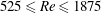 $525\leqslant \mathit{Re}\leqslant 1875$
. In DNS at
$525\leqslant \mathit{Re}\leqslant 1875$
. In DNS at
 $\mathit{Re}=4500$
, Schäfer et al. (Reference Schäfer, Breuer and Durst2009) found that the vortical structures associated with vortex shedding are responsible for the flapping of the separation lines and reattachment lines of the primary and secondary bubbles. In the current work, the generation of vortical structures between the main stream and the bubbles is investigated so as to identify the source of vortex shedding and flapping.
$\mathit{Re}=4500$
, Schäfer et al. (Reference Schäfer, Breuer and Durst2009) found that the vortical structures associated with vortex shedding are responsible for the flapping of the separation lines and reattachment lines of the primary and secondary bubbles. In the current work, the generation of vortical structures between the main stream and the bubbles is investigated so as to identify the source of vortex shedding and flapping.
Receptivity of the flow past a backward-facing step to inflow noise has been widely observed. High sensitivity of the flow downstream of the step with respect to the type of inflow boundary condition has been reported (Kaltenbach & Janke Reference Kaltenbach and Janke2000; Schäfer et al. Reference Schäfer, Breuer and Durst2009), and strong correlations between the frequency of the inflow noise and the oscillation of the shear layers downstream of the step have been observed (Kaiktsis et al. Reference Kaiktsis, Karniadakis and Orszag1996). It has been argued that the combination of inflow disturbances and shear layer instabilities, e.g. Kelvin–Helmholtz instabilities, triggers the three-dimensional vortical structures (Yanase et al. Reference Yanase, Kawahara and Kiyama2001). However, in all these works, the distribution of the inflow noise is either empirically prescribed or random, whereas in the current work, the optimal (most energetic) inflow perturbation will be calculated and its relation to vortex shedding, flapping of the bubbles and three-dimensionality will be explored.
Control of the flow past a backward-facing step using blowing/suction or geometry variations, which can be interpreted as base flow modifications, has been discussed mostly in the context of attempting to enhance noise amplifications. A combination of suction on the step face and blowing downstream of the step has been used to destabilize the flow and enhance mixing in the channel (Kaiktsis & Monkewitz Reference Kaiktsis and Monkewitz2003). It has also been suggested that the destabilized two-dimensional flow is subject to three-dimensional secondary instabilities. Similar destabilization and enhancement of mixing was obtained by modulating the flow using spanwise-distributed roughness elements upstream of the step (Boiko et al. Reference Boiko, Dovgal and Sorokin2012) or tabs on the edges of the step (Park et al. Reference Park, Jeon, Choi and Yoo2007). These previous control or base flow modification studies all aim at activating instabilities and turbulence, whereas in the current work, the base flow modification generated by the linearly optimal body force can either suppress or enhance the noise amplifications, depending on the choice of a scale factor that measures the size and sign of the body force.
The remainder of this paper is organized as follows. In § 2, the method used to calculate the optimal base flow modification induced by the body force is demonstrated. Then, after a convergence test in § 3, the receptivity of flow past a backward-facing step to inflow noise is presented in § 4. The optimal modification of the base flow with respect to the receptivity is further studied in § 5, and the correlation between the receptivities to inflow and initial perturbations is discussed in § 6. Finally, conclusions are drawn in § 7.
2. Methodology
In this section, we present the method used to calculate the body force that (in the linear regime) optimally modifies the base flow. The perturbations and their development are modelled in § 2.1; the definitions of noise amplifications are presented in § 2.2; a Lagrangian functional is defined in § 2.3, and based on this Lagrangian, the formulation of the optimal body force is derived in § 2.4; finally, the calculation procedure is summarized in § 2.5.
2.1. Governing equations
For flow past a backward-facing step, assuming the fluid to be incompressible, the governing equations, i.e. the incompressible NS equations, can be written as
 $$\begin{eqnarray}\partial _{t}\hat{\boldsymbol{u}}+\hat{\boldsymbol{u}}\boldsymbol{\cdot }\boldsymbol{{\rm\nabla}}\hat{\boldsymbol{u}}+\boldsymbol{{\rm\nabla}}\hat{p}-\mathit{Re}^{-1}{\rm\nabla}^{2}\hat{\boldsymbol{u}}=\boldsymbol{f}\quad \text{with }\boldsymbol{{\rm\nabla}}\boldsymbol{\cdot }\hat{\boldsymbol{u}}=0,\end{eqnarray}$$
where
 $\mathit{Re}$
is the Reynolds number defined using the maximum inflow velocity and the step height (we use
$\mathit{Re}$
is the Reynolds number defined using the maximum inflow velocity and the step height (we use
 $\mathit{Re}=500$
throughout this work if not otherwise stated),
$\mathit{Re}=500$
throughout this work if not otherwise stated),
 $\hat{\boldsymbol{u}}$
is the velocity vector,
$\hat{\boldsymbol{u}}$
is the velocity vector,
 $\hat{p}$
is the kinematic pressure and
$\hat{p}$
is the kinematic pressure and
 $\boldsymbol{f}$
denotes the body force. On the inflow boundary, appropriate Dirichlet velocity conditions (a perturbed parabolic profile in this work) are imposed, as will be described in detail below; on the wall boundary, no-slip velocity conditions are adopted; and on the outflow boundary, zero Dirichlet and zero Neumann conditions are implemented for the velocity and pressure terms, respectively. A computed Neumann pressure condition is applied if the velocity boundary condition is of Dirichlet type (Karniadakis, Israeli & Orszag Reference Karniadakis, Israeli and Orszag1991). These equations are compactly written as
$\boldsymbol{f}$
denotes the body force. On the inflow boundary, appropriate Dirichlet velocity conditions (a perturbed parabolic profile in this work) are imposed, as will be described in detail below; on the wall boundary, no-slip velocity conditions are adopted; and on the outflow boundary, zero Dirichlet and zero Neumann conditions are implemented for the velocity and pressure terms, respectively. A computed Neumann pressure condition is applied if the velocity boundary condition is of Dirichlet type (Karniadakis, Israeli & Orszag Reference Karniadakis, Israeli and Orszag1991). These equations are compactly written as
 $$\begin{eqnarray}\partial _{t}\hat{\boldsymbol{u}}+D\hat{\boldsymbol{u}}=\boldsymbol{f}\end{eqnarray}$$
in the following, where
 $D$
is a nonlinear operator whose linear counterpart has been much used in hydrodynamic stability analyses, as will be presented below.
$D$
is a nonlinear operator whose linear counterpart has been much used in hydrodynamic stability analyses, as will be presented below.
At
 $\mathit{Re}=500$
, the flow past a backward-facing step is a strong noise amplifier (Blackburn et al.
Reference Blackburn, Barkley and Sherwin2008), and therefore the solution of the NS equations can be unsteady if perturbations (e.g. initial perturbations, boundary perturbations or external forcing) are introduced into the computational domain. However, by integrating the NS equations over a long enough time period to ‘wash out’ the initial perturbations and specifying a zero body force and an appropriate steady inflow boundary condition (e.g. a parabolic velocity profile), a steady solution can be obtained. Such a steady solution, referred to as the base flow, is subject to perturbations such as boundary perturbations and initial perturbations. Therefore, the ‘real’ flow can be decomposed as the sum of the base flow and the perturbation flow, i.e.
$\mathit{Re}=500$
, the flow past a backward-facing step is a strong noise amplifier (Blackburn et al.
Reference Blackburn, Barkley and Sherwin2008), and therefore the solution of the NS equations can be unsteady if perturbations (e.g. initial perturbations, boundary perturbations or external forcing) are introduced into the computational domain. However, by integrating the NS equations over a long enough time period to ‘wash out’ the initial perturbations and specifying a zero body force and an appropriate steady inflow boundary condition (e.g. a parabolic velocity profile), a steady solution can be obtained. Such a steady solution, referred to as the base flow, is subject to perturbations such as boundary perturbations and initial perturbations. Therefore, the ‘real’ flow can be decomposed as the sum of the base flow and the perturbation flow, i.e.
 $(\hat{\boldsymbol{u}},\hat{p})=(\boldsymbol{U},P)+(\boldsymbol{u},p)$
, where
$(\hat{\boldsymbol{u}},\hat{p})=(\boldsymbol{U},P)+(\boldsymbol{u},p)$
, where
 $(\boldsymbol{U},P)$
denote the base flow velocity and pressure, respectively, and
$(\boldsymbol{U},P)$
denote the base flow velocity and pressure, respectively, and
 $(\boldsymbol{u},p)$
represent the perturbation velocity and pressure, respectively.
$(\boldsymbol{u},p)$
represent the perturbation velocity and pressure, respectively.
If the magnitude of the perturbation is small relative to the base flow, the development of perturbations is governed by the linearized NS equations
 $$\begin{eqnarray}\partial _{t}\boldsymbol{u}+\boldsymbol{U}\boldsymbol{\cdot }\boldsymbol{{\rm\nabla}}\boldsymbol{u}+(\boldsymbol{{\rm\nabla}}\boldsymbol{U})^{\text{T}}\boldsymbol{\cdot }\boldsymbol{u}+\boldsymbol{{\rm\nabla}}p-\mathit{Re}^{-1}{\rm\nabla}^{2}\boldsymbol{u}=0\quad \text{with }\boldsymbol{{\rm\nabla}}\boldsymbol{\cdot }\boldsymbol{u}=0\end{eqnarray}$$
or, more compactly,
 $$\begin{eqnarray}\partial _{t}\boldsymbol{u}-L(\boldsymbol{U})\boldsymbol{u}=0,\end{eqnarray}$$
where
 $L(\boldsymbol{U})$
is the linearized operator of
$L(\boldsymbol{U})$
is the linearized operator of
 $D$
, which depends on the base flow and acts on the perturbation. This operator has been extensively used in stability and non-normality studies (Trefethen et al.
Reference Trefethen, Trefethen, Reddy and Driscoll1993; Chomaz Reference Chomaz2005; Schmid Reference Schmid2007). The boundary conditions for the linearized NS equations are the same as those for the NS equations (2.2), except that on the inflow boundary a velocity perturbation is imposed after decoupling the unperturbed parabolic profile from the perturbed inflow velocity condition.
$D$
, which depends on the base flow and acts on the perturbation. This operator has been extensively used in stability and non-normality studies (Trefethen et al.
Reference Trefethen, Trefethen, Reddy and Driscoll1993; Chomaz Reference Chomaz2005; Schmid Reference Schmid2007). The boundary conditions for the linearized NS equations are the same as those for the NS equations (2.2), except that on the inflow boundary a velocity perturbation is imposed after decoupling the unperturbed parabolic profile from the perturbed inflow velocity condition.
The perturbations may stem from either boundary perturbations or initial perturba- tions. An initial perturbation can be modelled as an initial condition of the linearized NS equations, denoted by
 $\boldsymbol{u}_{0}$
. Correspondingly, a boundary perturbation can be modelled as a boundary condition of the linearized NS equations, denoted by
$\boldsymbol{u}_{0}$
. Correspondingly, a boundary perturbation can be modelled as a boundary condition of the linearized NS equations, denoted by
 $\boldsymbol{u}_{b}(\boldsymbol{x},t)$
, where
$\boldsymbol{u}_{b}(\boldsymbol{x},t)$
, where
 $\boldsymbol{x}$
represents the coordinate of the perturbation boundary. To reduce the dimension of
$\boldsymbol{x}$
represents the coordinate of the perturbation boundary. To reduce the dimension of
 $\boldsymbol{u}_{b}(\boldsymbol{x},t)$
after temporal–spatial discretization, decompose the temporal and spatial dependence as
$\boldsymbol{u}_{b}(\boldsymbol{x},t)$
after temporal–spatial discretization, decompose the temporal and spatial dependence as
 $$\begin{eqnarray}\boldsymbol{u}_{b}(\boldsymbol{x},t)=\tilde{\boldsymbol{u}}_{b}(\boldsymbol{x})T(t,{\it\omega}),\end{eqnarray}$$
where
 $\tilde{\boldsymbol{u}}_{b}(\boldsymbol{x})$
is the spatial dependence and
$\tilde{\boldsymbol{u}}_{b}(\boldsymbol{x})$
is the spatial dependence and
 $T(t,{\it\omega})$
is a prescribed temporal-dependence function,
$T(t,{\it\omega})$
is a prescribed temporal-dependence function,
 $$\begin{eqnarray}T(t,{\it\omega})=(1-\text{e}^{-{\it\sigma}t^{2}})[1-\text{e}^{-{\it\sigma}({\it\tau}-t)^{2}}]\text{e}^{\text{i}{\it\omega}t},\end{eqnarray}$$
with
 ${\it\tau}$
being the final time and
${\it\tau}$
being the final time and
 ${\it\sigma}$
a positive relaxation factor. The first two factors in (2.6) ensure that
${\it\sigma}$
a positive relaxation factor. The first two factors in (2.6) ensure that
 $\boldsymbol{u}_{b}(\boldsymbol{x},0)=0$
and
$\boldsymbol{u}_{b}(\boldsymbol{x},0)=0$
and
 $\boldsymbol{u}_{b}(\boldsymbol{x},{\it\tau})=0$
, in order to eliminate the temporal and spatial discontinuity at the beginning of the integration of the linearized NS equations and the adjoint equation (which will be introduced later in (2.12)), and the last factor specifies the frequency of the inflow perturbation to be
$\boldsymbol{u}_{b}(\boldsymbol{x},{\it\tau})=0$
, in order to eliminate the temporal and spatial discontinuity at the beginning of the integration of the linearized NS equations and the adjoint equation (which will be introduced later in (2.12)), and the last factor specifies the frequency of the inflow perturbation to be
 ${\it\omega}$
as the final time tends to infinity. It is seen that for increasing
${\it\omega}$
as the final time tends to infinity. It is seen that for increasing
 ${\it\sigma}$
,
${\it\sigma}$
,
 $T(t,{\it\omega})\rightarrow \text{e}^{\text{i}{\it\omega}t}$
. However, a large value of
$T(t,{\it\omega})\rightarrow \text{e}^{\text{i}{\it\omega}t}$
. However, a large value of
 ${\it\sigma}$
induces a high gradient of
${\it\sigma}$
induces a high gradient of
 $T(t,{\it\omega})$
or
$T(t,{\it\omega})$
or
 $\boldsymbol{u}_{b}(\boldsymbol{x},t)$
with respect to
$\boldsymbol{u}_{b}(\boldsymbol{x},t)$
with respect to
 $t$
at
$t$
at
 $t=0$
, and therefore leads to numerical discontinuity. The choice of this relaxation factor will be discussed in detail in § 3. In the present work, the inflow boundary is considered as the perturbation boundary in order to model the upstream noise. Under the linear assumption that the perturbations are small enough, the developments of the boundary and initial perturbations are decoupled and hence can be considered separately.
$t=0$
, and therefore leads to numerical discontinuity. The choice of this relaxation factor will be discussed in detail in § 3. In the present work, the inflow boundary is considered as the perturbation boundary in order to model the upstream noise. Under the linear assumption that the perturbations are small enough, the developments of the boundary and initial perturbations are decoupled and hence can be considered separately.
To simplify notation, introduce the scalar products
 $$\begin{eqnarray}(\boldsymbol{a},\boldsymbol{b})=\int _{{\it\Omega}}\boldsymbol{a}\boldsymbol{\cdot }\boldsymbol{b}\hspace{2.22198pt}\text{d}V,\quad \langle \boldsymbol{a},\boldsymbol{b}\rangle ={\it\tau}^{-1}\int _{0}^{{\it\tau}}(\boldsymbol{a},\boldsymbol{b})\,\text{d}t,\quad [\boldsymbol{c},\boldsymbol{d}]=\int _{\partial {\it\Omega}_{b}}\boldsymbol{c}\boldsymbol{\cdot }\boldsymbol{d}\hspace{2.22198pt}\text{d}S,\end{eqnarray}$$
where
 ${\it\Omega}$
represents the spatial domain,
${\it\Omega}$
represents the spatial domain,
 $\partial {\it\Omega}_{b}$
denotes the perturbation boundary, which refers to the inflow boundary in this work,
$\partial {\it\Omega}_{b}$
denotes the perturbation boundary, which refers to the inflow boundary in this work,
 $\boldsymbol{a}$
and
$\boldsymbol{a}$
and
 $\boldsymbol{b}$
are defined on the domain
$\boldsymbol{b}$
are defined on the domain
 ${\it\Omega}$
and
${\it\Omega}$
and
 $\boldsymbol{c}$
and
$\boldsymbol{c}$
and
 $\boldsymbol{d}$
are defined on the perturbation boundary
$\boldsymbol{d}$
are defined on the perturbation boundary
 $\partial {\it\Omega}_{b}$
.
$\partial {\it\Omega}_{b}$
.
2.2. Receptivity to inflow and initial perturbations
The receptivity of the base flow to inflow perturbations can be quantified as the gain
 $$\begin{eqnarray}K\equiv \text{max}_{\tilde{\boldsymbol{u}}_{b}}\frac{(\boldsymbol{u}_{{\it\tau}},\boldsymbol{u}_{{\it\tau}})}{[\tilde{\boldsymbol{u}}_{b},\tilde{\boldsymbol{u}}_{b}]},\end{eqnarray}$$
where
 $\boldsymbol{u}_{{\it\tau}}$
denotes the perturbation velocity at the final time. From the definition, the gain
$\boldsymbol{u}_{{\it\tau}}$
denotes the perturbation velocity at the final time. From the definition, the gain
 $K$
represents the largest amplification of the base flow to all possible inflow boundary perturbations for a given final time and inflow frequency. The boundary perturbation at which
$K$
represents the largest amplification of the base flow to all possible inflow boundary perturbations for a given final time and inflow frequency. The boundary perturbation at which
 $K$
is obtained is referred to as the optimal boundary perturbation. In this definition, the initial perturbation is set to zero. The method for calculating
$K$
is obtained is referred to as the optimal boundary perturbation. In this definition, the initial perturbation is set to zero. The method for calculating
 $K$
and the associated optimal boundary perturbation has been presented in Mao et al. (Reference Mao, Blackburn and Sherwin2013).
$K$
and the associated optimal boundary perturbation has been presented in Mao et al. (Reference Mao, Blackburn and Sherwin2013).
Correspondingly, the receptivity to initial perturbations or transient energy growth can be quantified by the gain
 $$\begin{eqnarray}G\equiv \text{max}_{\boldsymbol{u}_{0}}\frac{(\boldsymbol{u}_{{\it\tau}},\boldsymbol{u}_{{\it\tau}})}{(\boldsymbol{u}_{0},\boldsymbol{u}_{0})},\end{eqnarray}$$
where
 $G$
represents the maximum ratio of the final energy to the initial energy over the time period considered. The initial perturbation at which the gain
$G$
represents the maximum ratio of the final energy to the initial energy over the time period considered. The initial perturbation at which the gain
 $G$
is obtained is the optimal initial perturbation. In this definition, the boundary perturbations are set to zero. The method for calculating
$G$
is obtained is the optimal initial perturbation. In this definition, the boundary perturbations are set to zero. The method for calculating
 $G$
and the optimal initial perturbation is well established (Barkley, Blackburn & Sherwin Reference Barkley, Blackburn and Sherwin2008) and has been applied to flow past a backward-facing step by Blackburn et al. (Reference Blackburn, Barkley and Sherwin2008).
$G$
and the optimal initial perturbation is well established (Barkley, Blackburn & Sherwin Reference Barkley, Blackburn and Sherwin2008) and has been applied to flow past a backward-facing step by Blackburn et al. (Reference Blackburn, Barkley and Sherwin2008).
2.3. Lagrangian functional for base flow modifications
To investigate the effects of base flow modifications on noise amplification, variational techniques are employed (Bottaro et al. Reference Bottaro, Corbett and Luchini2003; Schmid Reference Schmid2007; Marquet et al. Reference Marquet, Sipp and Jacquin2008b ; Brandt et al. Reference Brandt, Sipp, Pralits and Marquet2011). Define the Lagrangian functional as
 $$\begin{eqnarray}\mathscr{L}=\text{gain}-\langle \boldsymbol{u}^{\ast },\partial _{t}\boldsymbol{u}-L(\boldsymbol{U})\boldsymbol{u}\rangle +({\bf\lambda},D\boldsymbol{U}-\boldsymbol{f}),\end{eqnarray}$$
where the gain is
 $K$
for boundary perturbation studies and
$K$
for boundary perturbation studies and
 $G$
for initial perturbation studies, as defined in (2.8) and (2.9), respectively; the second term, with
$G$
for initial perturbation studies, as defined in (2.8) and (2.9), respectively; the second term, with
 $\boldsymbol{u}^{\ast }$
being the adjoint velocity, is a constraint specifying that the perturbation should satisfy the linearized NS equations; the third term, with
$\boldsymbol{u}^{\ast }$
being the adjoint velocity, is a constraint specifying that the perturbation should satisfy the linearized NS equations; the third term, with
 ${\bf\lambda}$
being a Lagrange multiplier, is a constraint specifying that the base flow should satisfy the steady NS equations. It is worth noting that the last term involves the nonlinear NS equations, which will be linearized when calculating the linear sensitivity of the Lagrangian functional with respect to the base flow. This nonlinear form is adopted to facilitate the identification of nonlinear saturation of the body force effects, which involves solving the nonlinear forced NS equations. From the definitions of the nonlinear operator
${\bf\lambda}$
being a Lagrange multiplier, is a constraint specifying that the base flow should satisfy the steady NS equations. It is worth noting that the last term involves the nonlinear NS equations, which will be linearized when calculating the linear sensitivity of the Lagrangian functional with respect to the base flow. This nonlinear form is adopted to facilitate the identification of nonlinear saturation of the body force effects, which involves solving the nonlinear forced NS equations. From the definitions of the nonlinear operator
 $D$
(see (2.2)) and the linear operator
$D$
(see (2.2)) and the linear operator
 $L$
(see (2.4)), note that the divergence-free conditions for the base flow
$L$
(see (2.4)), note that the divergence-free conditions for the base flow
 $\boldsymbol{U}$
and perturbation
$\boldsymbol{U}$
and perturbation
 $\boldsymbol{u}$
have been imposed as constraints in this Lagrangian functional. For boundary perturbation studies the initial perturbation is set to zero, while for initial perturbation studies the boundary perturbation is set to zero.
$\boldsymbol{u}$
have been imposed as constraints in this Lagrangian functional. For boundary perturbation studies the initial perturbation is set to zero, while for initial perturbation studies the boundary perturbation is set to zero.
One may integrate the second term of (2.10) by parts to obtain
 $$\begin{eqnarray}\mathscr{L}=\text{gain}+\langle \boldsymbol{u},\partial _{t}\boldsymbol{u}^{\ast }+L^{\ast }(\boldsymbol{U})\boldsymbol{u}^{\ast }\rangle -(\boldsymbol{u}_{{\it\tau}},\boldsymbol{u}_{{\it\tau}}^{\ast })+(\boldsymbol{u}_{0},\boldsymbol{u}_{0}^{\ast })+[g(\boldsymbol{u}^{\ast }),\tilde{\boldsymbol{u}}_{b}]+({\bf\lambda},D\boldsymbol{U}-\boldsymbol{f}),\end{eqnarray}$$
where
 $L^{\ast }$
is the adjoint operator of
$L^{\ast }$
is the adjoint operator of
 $L$
and
$L$
and
 $$\begin{eqnarray}\partial _{t}\boldsymbol{u}^{\ast }+L^{\ast }(\boldsymbol{U})\boldsymbol{u}^{\ast }=0\end{eqnarray}$$
represents the adjoint equation, which is used extensively in non-normality studies and can be expanded as
 $$\begin{eqnarray}\partial _{t}\boldsymbol{u}^{\ast }+\boldsymbol{U}\boldsymbol{\cdot }\boldsymbol{{\rm\nabla}}\boldsymbol{u}^{\ast }-\boldsymbol{{\rm\nabla}}\boldsymbol{U}\boldsymbol{\cdot }\boldsymbol{u}^{\ast }-\boldsymbol{{\rm\nabla}}p^{\ast }+\mathit{Re}^{-1}{\rm\nabla}^{2}\boldsymbol{u}^{\ast }=0\quad \text{with}~\boldsymbol{{\rm\nabla}}\boldsymbol{\cdot }\boldsymbol{u}^{\ast }=0.\end{eqnarray}$$
We remark that this adjoint equation is integrated backwards in time (Barkley et al.
Reference Barkley, Blackburn and Sherwin2008). In (2.11),
 $\boldsymbol{u}_{{\it\tau}}^{\ast }$
and
$\boldsymbol{u}_{{\it\tau}}^{\ast }$
and
 $\boldsymbol{u}_{{\it\tau}}$
denote the adjoint velocity at
$\boldsymbol{u}_{{\it\tau}}$
denote the adjoint velocity at
 $t={\it\tau}$
and
$t={\it\tau}$
and
 $t=0$
respectively, and
$t=0$
respectively, and
 $\boldsymbol{g}(\boldsymbol{u}^{\ast })$
can be calculated by integrating the adjoint equation:
$\boldsymbol{g}(\boldsymbol{u}^{\ast })$
can be calculated by integrating the adjoint equation:
 $$\begin{eqnarray}\boldsymbol{g}(\boldsymbol{u}^{\ast })={\it\tau}^{-1}\int _{0}^{{\it\tau}}(p^{\ast }\boldsymbol{n}-\mathit{Re}^{-1}{\rm\nabla}_{\boldsymbol{ n}}\boldsymbol{u}^{\ast })T(t,-{\it\omega})\,\text{d}t,\end{eqnarray}$$
where
 ${\rm\nabla}_{\boldsymbol{n}}=\boldsymbol{n}\boldsymbol{\cdot }\boldsymbol{{\rm\nabla}}$
, with
${\rm\nabla}_{\boldsymbol{n}}=\boldsymbol{n}\boldsymbol{\cdot }\boldsymbol{{\rm\nabla}}$
, with
 $\boldsymbol{n}$
denoting the unit outward normal on the boundary. In this derivation, the inflow and wall boundary conditions for the adjoint velocity are set to zero; on the outflow, Robin velocity and zero Dirichlet pressure conditions are implemented (Mao et al.
Reference Mao, Blackburn and Sherwin2013).
$\boldsymbol{n}$
denoting the unit outward normal on the boundary. In this derivation, the inflow and wall boundary conditions for the adjoint velocity are set to zero; on the outflow, Robin velocity and zero Dirichlet pressure conditions are implemented (Mao et al.
Reference Mao, Blackburn and Sherwin2013).
2.4. Linearly optimal body force
The base flow can be modified directly or by adding a body force to the NS equations (Brandt et al. Reference Brandt, Sipp, Pralits and Marquet2011). A directly modified flow may violate the divergence-free condition, whereas the body-forced modification, obtained by integrating the forced NS equations, preserves the divergence-free condition. Therefore in this work the base flow modification will be generated by the body force, whose optimal distribution (i.e. the distribution which is most effective in modifying the base flow and its noise amplification characteristics) can be calculated through evaluating the gradient of the Lagrangian with respect to the body force.
Setting to zero the first variations of
 $\mathscr{L}$
with respect to
$\mathscr{L}$
with respect to
 $\boldsymbol{u}^{\ast }$
,
$\boldsymbol{u}^{\ast }$
,
 $\boldsymbol{u}$
and
$\boldsymbol{u}$
and
 ${\it\lambda}$
, we obtain that the perturbation, adjoint and base flow variables satisfy the linearized NS, adjoint and NS equations, respectively. Since the adjoint equation is integrated backwards, its initial condition is
${\it\lambda}$
, we obtain that the perturbation, adjoint and base flow variables satisfy the linearized NS, adjoint and NS equations, respectively. Since the adjoint equation is integrated backwards, its initial condition is
 $\boldsymbol{u}_{{\it\tau}}^{\ast }$
, which can be obtained by setting to zero the first variation of
$\boldsymbol{u}_{{\it\tau}}^{\ast }$
, which can be obtained by setting to zero the first variation of
 $\mathscr{L}$
with respect to
$\mathscr{L}$
with respect to
 $\boldsymbol{u}_{{\it\tau}}$
:
$\boldsymbol{u}_{{\it\tau}}$
:
 $$\begin{eqnarray}\boldsymbol{u}_{{\it\tau}}^{\ast }=\frac{2\boldsymbol{u}_{{\it\tau}}}{[\tilde{\boldsymbol{u}}_{b},\tilde{\boldsymbol{u}}_{b}]}\quad \text{or}\quad \boldsymbol{u}_{{\it\tau}}^{\ast }=\frac{2\boldsymbol{u}_{{\it\tau}}}{(\boldsymbol{u}_{0},\boldsymbol{u}_{0})}\end{eqnarray}$$
for the boundary perturbation or initial perturbation problem, respectively.
At the equilibrium state, where the Lagrangian reaches a maximum, for receptivity to inflow boundary perturbations,
 $\boldsymbol{u}_{0}$
is zero and
$\boldsymbol{u}_{0}$
is zero and
 $\tilde{\boldsymbol{u}}_{b}$
is the optimal boundary perturbation and parallel to
$\tilde{\boldsymbol{u}}_{b}$
is the optimal boundary perturbation and parallel to
 $g(\boldsymbol{u}^{\ast })$
(Mao et al.
Reference Mao, Blackburn and Sherwin2012), as can be seen by setting the variation with respect to
$g(\boldsymbol{u}^{\ast })$
(Mao et al.
Reference Mao, Blackburn and Sherwin2012), as can be seen by setting the variation with respect to
 $\tilde{\boldsymbol{u}}_{b}$
to zero. Correspondingly, for receptivity to initial perturbations,
$\tilde{\boldsymbol{u}}_{b}$
to zero. Correspondingly, for receptivity to initial perturbations,
 $\tilde{\boldsymbol{u}}_{b}$
is zero and
$\tilde{\boldsymbol{u}}_{b}$
is zero and
 $\boldsymbol{u}_{0}$
is parallel to
$\boldsymbol{u}_{0}$
is parallel to
 $\boldsymbol{u}_{0}^{\ast }$
, as can be obtained by setting the variation with respect to
$\boldsymbol{u}_{0}^{\ast }$
, as can be obtained by setting the variation with respect to
 $\boldsymbol{u}_{0}$
to zero.
$\boldsymbol{u}_{0}$
to zero.
Considering the Gâteaux differential as in Guégan et al. (Reference Guégan, Schmid and Huerre2006), the gradient of the Lagrangian with respect to the body force is
 $\boldsymbol{{\rm\nabla}}_{\boldsymbol{f}}\mathscr{L}={\bf\lambda}$
. Since the original body force used to calculate the base flow is zero (unforced), a linearly optimal body force that is most effective in modifying the receptivity is
$\boldsymbol{{\rm\nabla}}_{\boldsymbol{f}}\mathscr{L}={\bf\lambda}$
. Since the original body force used to calculate the base flow is zero (unforced), a linearly optimal body force that is most effective in modifying the receptivity is
 $$\begin{eqnarray}\boldsymbol{f}=0+r\frac{\boldsymbol{{\rm\nabla}}_{\boldsymbol{f}}\mathscr{L}}{(\boldsymbol{{\rm\nabla}}_{\boldsymbol{f}}\mathscr{L},\boldsymbol{{\rm\nabla}}_{\boldsymbol{f}}\mathscr{L})^{1/2}}=r\frac{{\bf\lambda}}{({\bf\lambda},{\bf\lambda})^{1/2}},\end{eqnarray}$$
where
 $r$
is a scale factor for the body force and
$r$
is a scale factor for the body force and
 $r^{2}$
represents the square integral of the body force in the computational domain. Therefore, the modified base flow obtained by driving the NS equations with the optimal body force can be considered as a function of
$r^{2}$
represents the square integral of the body force in the computational domain. Therefore, the modified base flow obtained by driving the NS equations with the optimal body force can be considered as a function of
 $r$
.
$r$
.
By setting the variation of the Lagrangian with respect to the base flow
 $\boldsymbol{U}$
to zero, it is seen that
$\boldsymbol{U}$
to zero, it is seen that
 ${\bf\lambda}$
satisfies
${\bf\lambda}$
satisfies
 $$\begin{eqnarray}L^{\ast }(\boldsymbol{U}){\bf\lambda}=\boldsymbol{F}\end{eqnarray}$$
where
 $$\begin{eqnarray}\boldsymbol{F}={\it\tau}^{-1}\int _{0}^{{\it\tau}}(-\boldsymbol{{\rm\nabla}}\boldsymbol{u}\boldsymbol{\cdot }\boldsymbol{u}^{\ast }+\boldsymbol{u}\boldsymbol{\cdot }\boldsymbol{{\rm\nabla}}\boldsymbol{u}^{\ast })\,\text{d}t/[\tilde{\boldsymbol{u}}_{b},\tilde{\boldsymbol{u}}_{b}].\end{eqnarray}$$
In this derivation, a term in
 $\boldsymbol{F}$
involving integration over all the boundaries, i.e.
$\boldsymbol{F}$
involving integration over all the boundaries, i.e.
 $-\!\int \boldsymbol{u}^{\ast }\boldsymbol{u}\boldsymbol{\cdot }\boldsymbol{n}\hspace{2.22198pt}\text{d}S$
, is dropped. This term is zero on the wall boundaries and inflow boundaries, but may not vanish on the outflow boundaries. Since
$-\!\int \boldsymbol{u}^{\ast }\boldsymbol{u}\boldsymbol{\cdot }\boldsymbol{n}\hspace{2.22198pt}\text{d}S$
, is dropped. This term is zero on the wall boundaries and inflow boundaries, but may not vanish on the outflow boundaries. Since
 $\boldsymbol{F}$
can be interpreted as the gradient of the Lagrangian with respect to the base flow (without the constraint of satisfying the NS equations), by further restricting the base flow modification to be inside the domain, this term becomes zero. As will be seen in the following sections, the base flow modification concentrates around the bubbles and is zero on the outflow boundary, confirming that this term can be dropped. If we adopt another, more complex, form of the Lagrangian functional (see appendix A), this term also vanishes, and the same result for the body force can be obtained.
$\boldsymbol{F}$
can be interpreted as the gradient of the Lagrangian with respect to the base flow (without the constraint of satisfying the NS equations), by further restricting the base flow modification to be inside the domain, this term becomes zero. As will be seen in the following sections, the base flow modification concentrates around the bubbles and is zero on the outflow boundary, confirming that this term can be dropped. If we adopt another, more complex, form of the Lagrangian functional (see appendix A), this term also vanishes, and the same result for the body force can be obtained.
Since the base flow is constrained to be steady, the body force
 $\boldsymbol{f}$
, and consequently
$\boldsymbol{f}$
, and consequently
 ${\bf\lambda}$
, should also be steady. Therefore
${\bf\lambda}$
, should also be steady. Therefore
 ${\bf\lambda}$
can be calculated as the steady solution of the forced adjoint equation
${\bf\lambda}$
can be calculated as the steady solution of the forced adjoint equation
 $$\begin{eqnarray}\partial _{t}{\bf\lambda}+L^{\ast }(\boldsymbol{U}){\bf\lambda}=\boldsymbol{F}.\end{eqnarray}$$
2.5. Calculation procedure
The procedure to calculate the optimal base flow modification with respect to receptivity to inflow noise can be summarized as follows.
-
(a) Calculate the unforced base flow
 $\boldsymbol{U}$
from the NS equations (2.2) with
$\boldsymbol{f}=0$
.
$\boldsymbol{U}$
from the NS equations (2.2) with
$\boldsymbol{f}=0$
. -
(b) Compute the optimal boundary perturbation with respect to the unforced base flow (Mao et al. Reference Mao, Blackburn and Sherwin2013).
-
(c) Integrate the linearized NS equations (2.4) and adjoint equation (2.12) to obtain
$\boldsymbol{u}(t)$
and
$\boldsymbol{u}^{\ast }(t)$
, and calculate the force
$\boldsymbol{F}$
using (2.18). -
(d) Integrate the forced adjoint equation (2.19) backwards over a long enough time until a steady solution for
${\bf\lambda}$
is obtained. -
(e) Substitute
${\bf\lambda}$
into (2.16) and choose a scale factor
$r$
for the body force to obtain a linearly optimal body force
$\boldsymbol{f}$
. -
(f) Substitute the optimal body force
$\boldsymbol{f}$
into the NS equations (2.2) and integrate over a long enough time until a steady forced solution is reached.


For initial perturbation problems, step (b) should be replaced with computing the optimal initial perturbations; all the subsequent steps remain the same.
The difference between the forced base flow and the unforced base flow can be interpreted as the base flow modification due to the linearly optimal body force. Then the effects of optimal base flow modifications on receptivity can be verified by comparing the gain
 $K$
(or
$K$
(or
 $G$
) based on the forced and unforced base flows.
$G$
) based on the forced and unforced base flows.
3. Discretization and validation
Spectral elements employing nodal-based polynomial expansions within quadrilateral elemental subdomains are used for the two-dimensional spatial discretization, combined with a Fourier decomposition in the spanwise direction. Time integration is carried out using a velocity-correction scheme. Details of the discretization and its convergence properties (exponential in spatial variables, second-order in time) are given in Blackburn & Sherwin (Reference Blackburn and Sherwin2004). The same numerical procedures are used to solve the NS, linearized NS and adjoint equations.
The computational domain and grid consisting of 992 spectral elements are shown in figure 1. The step is located at
 $x=0$
, and the outflow length (measured from the step to the outflow boundary) is 50, identical to the configuration used in a previous non-normality study (Blackburn et al.
Reference Blackburn, Barkley and Sherwin2008). The inflow boundary is located at
$x=0$
, and the outflow length (measured from the step to the outflow boundary) is 50, identical to the configuration used in a previous non-normality study (Blackburn et al.
Reference Blackburn, Barkley and Sherwin2008). The inflow boundary is located at
 $x=-5$
, which results in a shorter inflow length (measured from the inflow boundary to the step) than that used in Blackburn et al. (Reference Blackburn, Barkley and Sherwin2008), in order to isolate the step-induced dynamics from the upstream channel-induced dynamics. The inflow boundary is taken to be the perturbation boundary, without the uppermost and lowermost edges since these two edges are connected to the upper and lower walls, where no inflow noise should be introduced. Therefore the perturbation boundary is at
$x=-5$
, which results in a shorter inflow length (measured from the inflow boundary to the step) than that used in Blackburn et al. (Reference Blackburn, Barkley and Sherwin2008), in order to isolate the step-induced dynamics from the upstream channel-induced dynamics. The inflow boundary is taken to be the perturbation boundary, without the uppermost and lowermost edges since these two edges are connected to the upper and lower walls, where no inflow noise should be introduced. Therefore the perturbation boundary is at
 $x=-5$
and
$x=-5$
and
 $0.06\leqslant y\leqslant 0.94$
.
$0.06\leqslant y\leqslant 0.94$
.

Figure 1. Spectral elements in the computational domain: (a) overall domain; (b) domain close to the inflow boundary and the step.
In all the convergence investigations conducted in this section, we choose a large final time
 ${\it\tau}=150$
to eliminate transient effects. The frequency and the spanwise wavenumber of the boundary perturbation are set to
${\it\tau}=150$
to eliminate transient effects. The frequency and the spanwise wavenumber of the boundary perturbation are set to
 ${\it\omega}=0.5$
and
${\it\omega}=0.5$
and
 ${\it\beta}=0$
, where the gain
${\it\beta}=0$
, where the gain
 $K$
reaches a maximum, as will be discussed later in figure 4.
$K$
reaches a maximum, as will be discussed later in figure 4.
Convergence of the discretization is tested with respect to the spectral element decomposition and the polynomial order
 $P$
used in nodal expansions in each spectral element. Two grids are studied: grid A, as illustrated in figure 1, and grid B, which has the same domain but 2317 spectral elements. The relaxation factor
$P$
used in nodal expansions in each spectral element. Two grids are studied: grid A, as illustrated in figure 1, and grid B, which has the same domain but 2317 spectral elements. The relaxation factor
 ${\it\sigma}$
defined in (2.6) is set to
${\it\sigma}$
defined in (2.6) is set to
 $1$
in these convergence tests, and it has been observed that a further increase in
$1$
in these convergence tests, and it has been observed that a further increase in
 ${\it\sigma}$
changes the magnitude of noise amplifications slightly for final times
${\it\sigma}$
changes the magnitude of noise amplifications slightly for final times
 ${\it\tau}<70$
, at which the transient growth is evident, and has negligible effects for
${\it\tau}<70$
, at which the transient growth is evident, and has negligible effects for
 ${\it\tau}>70$
. As most of the following work focuses on a large final time at which transient effects vanish (i.e.
${\it\tau}>70$
. As most of the following work focuses on a large final time at which transient effects vanish (i.e.
 ${\it\tau}=150$
),
${\it\tau}=150$
),
 ${\it\sigma}=1$
is used throughout this work. As shown in table 1, the gain
${\it\sigma}=1$
is used throughout this work. As shown in table 1, the gain
 $K$
converges to a relative error of less than 0.4 % at
$K$
converges to a relative error of less than 0.4 % at
 $P=5$
for grid A with further refinements of the spatial discretization. It is also seen in table 1 that when the time step
$P=5$
for grid A with further refinements of the spatial discretization. It is also seen in table 1 that when the time step
 ${\rm\Delta}t$
is halved from 0.004 to 0.002, the relative change in
${\rm\Delta}t$
is halved from 0.004 to 0.002, the relative change in
 $K$
is less than 0.3 %. Therefore, in all the following integrations of the NS, linearized NS and adjoint equations, we use grid A with polynomial order
$K$
is less than 0.3 %. Therefore, in all the following integrations of the NS, linearized NS and adjoint equations, we use grid A with polynomial order
 $P=5$
and time step
$P=5$
and time step
 ${\rm\Delta}t=0.004$
.
${\rm\Delta}t=0.004$
.

Figure 2. Convergence of the gain with respect to the domain size.
Table 1. Convergence of the optimal gain
 $K$
with respect to the polynomial order
$K$
with respect to the polynomial order
 $P$
in the spectral element method, the grid (A or B) and the time step
$P$
in the spectral element method, the grid (A or B) and the time step
 ${\rm\Delta}t$
. The parameters are the Reynolds number
${\rm\Delta}t$
. The parameters are the Reynolds number
 $\mathit{Re}=500$
, the final time
$\mathit{Re}=500$
, the final time
 ${\it\tau}=150$
, the spanwise wavenumber
${\it\tau}=150$
, the spanwise wavenumber
 ${\it\beta}=0$
and the temporal frequency
${\it\beta}=0$
and the temporal frequency
 ${\it\omega}=0.5$
for inflow perturbation, as will be used in all the following convergence tests unless stated otherwise.
${\it\omega}=0.5$
for inflow perturbation, as will be used in all the following convergence tests unless stated otherwise.

Computational grids with longer inflow and outflow sections are generated to check the dependence of the gain on the domain size, as shown in figure 2. It is observed that the gain converges well with respect to the outflow length, and does not vary significantly with respect to the inflow length around the optimal frequency, i.e.
 ${\it\omega}=0.5$
. At higher frequencies, the inflow perturbation is more diffused in the inflow channel and therefore a longer inflow section reduces the gain
${\it\omega}=0.5$
. At higher frequencies, the inflow perturbation is more diffused in the inflow channel and therefore a longer inflow section reduces the gain
 $K$
.
$K$
.
The convergence of the optimal body force and the outcome of the optimal inflow perturbation are presented in table 2; the distribution of the optimal inflow perturbation will be discussed later in figure 5. The body force for extended domains, denoted by
 $\boldsymbol{f}_{i}$
, is projected to that for the default domain (with inflow length 5 and outflow length 50), represented by
$\boldsymbol{f}_{i}$
, is projected to that for the default domain (with inflow length 5 and outflow length 50), represented by
 $\boldsymbol{f}_{1}$
; so the convergence of
$\boldsymbol{f}_{1}$
; so the convergence of
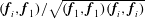 $(\boldsymbol{f}_{i},\boldsymbol{f}_{1})/\sqrt{(\boldsymbol{f}_{1},\boldsymbol{ f}_{1})(\boldsymbol{f}_{i},\boldsymbol{ f}_{i})}$
to 1 can be used as an indication of the similarity of the two body forces. It is seen that this indicator deviates from 1 within the discretization error for the four extended domains considered, suggesting that the optimal body force, which is the main focus of this work, is independent of further extensions of the domain. Similarly, it can be observed that a longer outflow or inflow section does not significantly change the distribution of the optimal outcome
$(\boldsymbol{f}_{i},\boldsymbol{f}_{1})/\sqrt{(\boldsymbol{f}_{1},\boldsymbol{ f}_{1})(\boldsymbol{f}_{i},\boldsymbol{ f}_{i})}$
to 1 can be used as an indication of the similarity of the two body forces. It is seen that this indicator deviates from 1 within the discretization error for the four extended domains considered, suggesting that the optimal body force, which is the main focus of this work, is independent of further extensions of the domain. Similarly, it can be observed that a longer outflow or inflow section does not significantly change the distribution of the optimal outcome
 $\boldsymbol{u}_{{\it\tau}}$
, as indicated by the value of
$\boldsymbol{u}_{{\it\tau}}$
, as indicated by the value of
 $(\boldsymbol{u}_{{\it\tau}i},\boldsymbol{u}_{{\it\tau}1})/\sqrt{(\boldsymbol{u}_{{\it\tau}1},\boldsymbol{ u}_{{\it\tau}1})(\boldsymbol{u}_{{\it\tau}i},\boldsymbol{ u}_{{\it\tau}i})}$
, where
$(\boldsymbol{u}_{{\it\tau}i},\boldsymbol{u}_{{\it\tau}1})/\sqrt{(\boldsymbol{u}_{{\it\tau}1},\boldsymbol{ u}_{{\it\tau}1})(\boldsymbol{u}_{{\it\tau}i},\boldsymbol{ u}_{{\it\tau}i})}$
, where
 $\boldsymbol{u}_{{\it\tau}i}$
and
$\boldsymbol{u}_{{\it\tau}i}$
and
 $\boldsymbol{u}_{{\it\tau}1}$
denote the outcomes at the extended and default domains, respectively.
$\boldsymbol{u}_{{\it\tau}1}$
denote the outcomes at the extended and default domains, respectively.

Figure 3. Contours of the streamwise velocity component of the base flow. The thick black lines represent the border streamlines of recirculation bubbles. The Reynolds number is fixed at
 $\mathit{Re}=500$
for this and all subsequent plots unless stated otherwise.
$\mathit{Re}=500$
for this and all subsequent plots unless stated otherwise.
Table 2. Convergence of the optimal body force
 $\boldsymbol{f}$
and the optimal outcome
$\boldsymbol{f}$
and the optimal outcome
 $\boldsymbol{u}_{{\it\tau}}$
with respect to the inflow and outflow lengths. The subscript
$\boldsymbol{u}_{{\it\tau}}$
with respect to the inflow and outflow lengths. The subscript
 $i$
denotes the
$i$
denotes the
 $i$
th case, e.g.
$i$
th case, e.g.
 $\boldsymbol{f}_{1}$
is the optimal body force for case 1.
$\boldsymbol{f}_{1}$
is the optimal body force for case 1.

4. Receptivity to inflow perturbations
The receptivity of the flow past a backward-facing step is studied first, before we address base flow modifications. Since the receptivity to initial perturbations in the backward-facing step flow has been thoroughly investigated but receptivity to inflow noise has received limited attention, in this section we focus on the receptivity to inflow perturbations. In § 4.1, the optimal gain and the corresponding optimal inflow perturbation are presented; in § 4.2, the mechanisms of receptivity are revealed; in § 4.3, the nonlinear development of the optimal inflow perturbation is studied; in § 4.4, random inflow noise is used to identify the role of optimal inflow perturbations in real conditions; finally, in § 4.5, the dependence of receptivity on the Reynolds number is examined.
4.1. Optimal inflow perturbation and its outcome
The unforced base flow (
 $\boldsymbol{f}=0$
) is illustrated in figure 3. Two recirculation bubbles, characterized by negative streamwise velocity, can be observed downstream of the step. The primary bubble is associated with the lower wall and reattaches around
$\boldsymbol{f}=0$
) is illustrated in figure 3. Two recirculation bubbles, characterized by negative streamwise velocity, can be observed downstream of the step. The primary bubble is associated with the lower wall and reattaches around
 $x=11$
, while the secondary bubble is associated with the upper wall, separates around
$x=11$
, while the secondary bubble is associated with the upper wall, separates around
 $x=8$
and reattaches around
$x=8$
and reattaches around
 $x=17$
. It can be seen that the flow is almost parallel downstream of the secondary bubble, which supports local, or streamwise-periodic, perturbation developments. This base flow is asymptotically stable but acts as an amplifier of upstream noise and exhibits strong transient energy growth (Blackburn et al.
Reference Blackburn, Barkley and Sherwin2008; Marquet et al.
Reference Marquet, Sipp and Jacquin2008b
).
$x=17$
. It can be seen that the flow is almost parallel downstream of the secondary bubble, which supports local, or streamwise-periodic, perturbation developments. This base flow is asymptotically stable but acts as an amplifier of upstream noise and exhibits strong transient energy growth (Blackburn et al.
Reference Blackburn, Barkley and Sherwin2008; Marquet et al.
Reference Marquet, Sipp and Jacquin2008b
).
The receptivity of this base flow to upstream noise, measured by the gain
 $K$
, at various spanwise wavenumbers
$K$
, at various spanwise wavenumbers
 ${\it\beta}$
, final times
${\it\beta}$
, final times
 ${\it\tau}$
and frequencies
${\it\tau}$
and frequencies
 ${\it\omega}$
is plotted in figure 4. It is seen that inflow perturbations with
${\it\omega}$
is plotted in figure 4. It is seen that inflow perturbations with
 ${\it\omega}=0.50$
are the most amplified, and the global maximum gain over the parameters considered occurs at
${\it\omega}=0.50$
are the most amplified, and the global maximum gain over the parameters considered occurs at
 ${\it\tau}=150$
,
${\it\tau}=150$
,
 ${\it\beta}=0$
and
${\it\beta}=0$
and
 ${\it\omega}=0.50$
. From the transient receptivity at
${\it\omega}=0.50$
. From the transient receptivity at
 ${\it\beta}=0$
, as shown in figure 4(a), it is observed that the transient effects vanish at
${\it\beta}=0$
, as shown in figure 4(a), it is observed that the transient effects vanish at
 ${\it\tau}=150$
(the gain becomes constant with respect to
${\it\tau}=150$
(the gain becomes constant with respect to
 ${\it\tau}$
). Since the transient noise amplification can be more clearly illustrated by the receptivity to initial perturbations, in all the following studies of receptivity to inflow noise we will use
${\it\tau}$
). Since the transient noise amplification can be more clearly illustrated by the receptivity to initial perturbations, in all the following studies of receptivity to inflow noise we will use
 ${\it\tau}=150$
unless stated otherwise, in order to exclude transient effects. In figure 4(b), one can see that the receptivity is maximized at
${\it\tau}=150$
unless stated otherwise, in order to exclude transient effects. In figure 4(b), one can see that the receptivity is maximized at
 ${\it\beta}=0$
and decreases almost monotonically with increasing
${\it\beta}=0$
and decreases almost monotonically with increasing
 ${\it\beta}$
, except that at small
${\it\beta}$
, except that at small
 ${\it\omega}$
the optimal value of
${\it\omega}$
the optimal value of
 ${\it\beta}$
is around 1.
${\it\beta}$
is around 1.

Figure 4. Contours of the gain
 $K$
at (a)
$K$
at (a)
 ${\it\beta}=0$
and (b)
${\it\beta}=0$
and (b)
 ${\it\tau}=150$
.
${\it\tau}=150$
.
In figure 5, the spatial distributions of the optimal inflow perturbation obtained at
 ${\it\beta}=0$
,
${\it\beta}=0$
,
 ${\it\tau}=150$
and three typical frequencies
${\it\tau}=150$
and three typical frequencies
 ${\it\omega}$
are displayed. It shows that the vertical wavenumber of the perturbation increases while the oscillation magnitude decreases with increasing
${\it\omega}$
are displayed. It shows that the vertical wavenumber of the perturbation increases while the oscillation magnitude decreases with increasing
 ${\it\omega}$
. For the global optimal inflow perturbation (
${\it\omega}$
. For the global optimal inflow perturbation (
 ${\it\omega}=0.5$
), the vertical component is significantly smaller than the streamwise component, and so this global optimal perturbation can be interpreted as a streamwise gust. It is also worth noting that the distribution of the optimal inflow noise is independent of further extensions of the outflow section, whereas for a longer inflow section, it tends to be a uniform streamwise perturbation. Such uniform inflow noise becomes optimal because it induces perturbations around the step with the same magnitude (considering the continuity and streamwise momentum equations), without being diffused in the elongated channel flow upstream of the step.
${\it\omega}=0.5$
), the vertical component is significantly smaller than the streamwise component, and so this global optimal perturbation can be interpreted as a streamwise gust. It is also worth noting that the distribution of the optimal inflow noise is independent of further extensions of the outflow section, whereas for a longer inflow section, it tends to be a uniform streamwise perturbation. Such uniform inflow noise becomes optimal because it induces perturbations around the step with the same magnitude (considering the continuity and streamwise momentum equations), without being diffused in the elongated channel flow upstream of the step.

Figure 5. Distribution of the optimal inflow velocity
 $\tilde{\boldsymbol{u}}_{b}$
at
$\tilde{\boldsymbol{u}}_{b}$
at
 ${\it\tau}=150$
and
${\it\tau}=150$
and
 ${\it\beta}=0$
: (a) streamwise velocity component; (b) vertical velocity component. The magnitude is normalized to satisfy
${\it\beta}=0$
: (a) streamwise velocity component; (b) vertical velocity component. The magnitude is normalized to satisfy
 $[\tilde{\boldsymbol{u}}_{b},\tilde{\boldsymbol{u}}_{b}]=1$
. The default inflow and outflow lengths are 5 and 50, respectively.
$[\tilde{\boldsymbol{u}}_{b},\tilde{\boldsymbol{u}}_{b}]=1$
. The default inflow and outflow lengths are 5 and 50, respectively.
Figure 6 displays the outcomes of the optimal inflow perturbations presented in figure 5. Since the distribution of the outcomes is independent of the domain size as shown in table 2, the optimal outcomes at various domain sizes are not reported here. The wavenumber of the perturbation in the streamwise direction roughly reflects the frequency of the inflow noise. It is worth noting that the outcome of the most energetic inflow perturbation at
 ${\it\omega}=0.5$
is concentrated in the region downstream of the secondary bubble, with the magnitude of the inflow perturbation velocity being amplified over two orders of magnitude, while the outcomes at
${\it\omega}=0.5$
is concentrated in the region downstream of the secondary bubble, with the magnitude of the inflow perturbation velocity being amplified over two orders of magnitude, while the outcomes at
 ${\it\omega}=0$
and 1.5 are associated with the primary bubble and the fore part of the secondary bubble. For the three outcomes, the structures upstream of the end of the secondary bubble are dominated by strings of vorticity, whose sign changes around the bubble borders, thus manifesting the inflectional point instability associated with shear layers in recirculation bubbles (Marquet et al.
Reference Marquet, Sipp, Chomaz and Jacquin2008a
). For the two non-zero-frequency cases, induced perturbations with smaller magnitudes around the upper and lower walls are also observed.
${\it\omega}=0$
and 1.5 are associated with the primary bubble and the fore part of the secondary bubble. For the three outcomes, the structures upstream of the end of the secondary bubble are dominated by strings of vorticity, whose sign changes around the bubble borders, thus manifesting the inflectional point instability associated with shear layers in recirculation bubbles (Marquet et al.
Reference Marquet, Sipp, Chomaz and Jacquin2008a
). For the two non-zero-frequency cases, induced perturbations with smaller magnitudes around the upper and lower walls are also observed.

Figure 6. Contours of spanwise vorticity for the outcomes of the optimal inflow boundary perturbations at
 $t=150$
,
$t=150$
,
 ${\it\beta}=0$
,
${\it\beta}=0$
,
 ${\it\tau}=150$
and (a)
${\it\tau}=150$
and (a)
 ${\it\omega}=0$
, (b)
${\it\omega}=0$
, (b)
 ${\it\omega}=0.5$
or (c)
${\it\omega}=0.5$
or (c)
 ${\it\omega}=1.5$
. The inflow perturbation is normalized so that
${\it\omega}=1.5$
. The inflow perturbation is normalized so that
 $[\tilde{\boldsymbol{u}}_{b},\tilde{\boldsymbol{u}}_{b}]=1$
. The thick black lines represent the borders of recirculation bubbles.
$[\tilde{\boldsymbol{u}}_{b},\tilde{\boldsymbol{u}}_{b}]=1$
. The thick black lines represent the borders of recirculation bubbles.
4.2. Mechanisms of receptivity
To illustrate the mechanisms underlying receptivity, consider as an example the case where
 ${\it\beta}=0$
,
${\it\beta}=0$
,
 ${\it\tau}=150$
and
${\it\tau}=150$
and
 ${\it\omega}=0.5$
, at which the receptivity reaches a maximum. From the momentum equation of perturbations, we have
${\it\omega}=0.5$
, at which the receptivity reaches a maximum. From the momentum equation of perturbations, we have
 $$\begin{eqnarray}\partial _{t}\frac{\boldsymbol{u}\boldsymbol{\cdot }\boldsymbol{u}}{2}+\boldsymbol{{\rm\nabla}}\boldsymbol{\cdot }\left(\boldsymbol{U}\frac{\boldsymbol{u}\boldsymbol{\cdot }\boldsymbol{u}}{2}\right)+\boldsymbol{u}\boldsymbol{\cdot }\boldsymbol{{\rm\nabla}}\boldsymbol{U}\boldsymbol{\cdot }\boldsymbol{u}+\boldsymbol{{\rm\nabla}}\boldsymbol{\cdot }(\boldsymbol{u}p)=0.\end{eqnarray}$$
In this derivation, the viscous diffusion is neglected and the divergence-free conditions on both the perturbation flow and the base flow are used.
In the region downstream of the secondary bubble, the base flow is almost parallel (see figure 3). Neglecting the vertical component of the base velocity and the streamwise gradient of the streamwise base velocity, we obtain
 $$\begin{eqnarray}\boldsymbol{u}\boldsymbol{\cdot }\boldsymbol{{\rm\nabla}}\boldsymbol{U}\boldsymbol{\cdot }\boldsymbol{u}=uv\frac{\text{d}U}{\text{d}y},\end{eqnarray}$$
where
 $u$
,
$u$
,
 $v$
and
$v$
and
 $U$
are the streamwise perturbation velocity, vertical perturbation velocity and streamwise base velocity, respectively.
$U$
are the streamwise perturbation velocity, vertical perturbation velocity and streamwise base velocity, respectively.
Note that in the region downstream of the secondary bubble, the perturbations are approximately periodic in the streamwise direction (see figure 6 b), manifesting the local dynamics. Therefore the integrals of the second and fourth terms in (4.1) over a section of the domain covering a period of the perturbations vanish:
 $$\begin{eqnarray}\int \boldsymbol{{\rm\nabla}}\boldsymbol{\cdot }\left(\boldsymbol{U}\frac{\boldsymbol{u}\boldsymbol{\cdot }\boldsymbol{u}}{2}+\boldsymbol{u}p\right)\text{d}V=\int \boldsymbol{n}\boldsymbol{\cdot }\left(\boldsymbol{U}\frac{\boldsymbol{u}\boldsymbol{\cdot }\boldsymbol{u}}{2}+\boldsymbol{u}p\right)\text{d}S=0,\end{eqnarray}$$
since the velocities are zero on the wall boundary and are the same on the inflow and outflow boundaries of the selected domain, whose surface normal
 $\boldsymbol{n}$
is opposite.
$\boldsymbol{n}$
is opposite.
Combining (4.1)–(4.3), we obtain the energy equation of the perturbations,
 $$\begin{eqnarray}\text{d}E/\text{d}t=-\int uv\frac{\text{d}U}{\text{d}y}\,\text{d}V,\end{eqnarray}$$
in a similar way to the derivation for a vortex flow in a cylindrical frame (Pradeep & Hussain Reference Pradeep and Hussain2006). Here
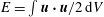 $E=\int \boldsymbol{u}\boldsymbol{\cdot }\boldsymbol{u}/2\,\text{d}V$
is the perturbation energy in this region, whose streamwise extension covers one period of the perturbations.
$E=\int \boldsymbol{u}\boldsymbol{\cdot }\boldsymbol{u}/2\,\text{d}V$
is the perturbation energy in this region, whose streamwise extension covers one period of the perturbations.
On the upper part of the channel,
 $\text{d}U/\text{d}y<0$
, and on the lower part
$\text{d}U/\text{d}y<0$
, and on the lower part
 $\text{d}U/\text{d}y>0$
. Therefore, as shown in figure 7, a perturbation with left-headed streamlines (bending to the left) results in
$\text{d}U/\text{d}y>0$
. Therefore, as shown in figure 7, a perturbation with left-headed streamlines (bending to the left) results in
 $uv(\text{d}U/\text{d}y)<0$
, with energy growing according to (4.4); a perturbation with right-headed streamlines (bending to the right) corresponds to
$uv(\text{d}U/\text{d}y)<0$
, with energy growing according to (4.4); a perturbation with right-headed streamlines (bending to the right) corresponds to
 $uv(\text{d}U/\text{d}y)>0$
and decays in time; a rectangular streamline is neutral (i.e. neither grows nor decays, provided that viscous diffusion is neglected).
$uv(\text{d}U/\text{d}y)>0$
and decays in time; a rectangular streamline is neutral (i.e. neither grows nor decays, provided that viscous diffusion is neglected).

Figure 7. Perturbation streamlines that result in energy growth and decay in a parallel base flow. The solid lines with arrows represent the base flow streamwise velocity, and the dashed lines with arrows represent streamlines of the perturbation. The dotted horizontal line is the centreline of the channel, and the solid horizontal and vertical lines delineate the border of a segment of the domain under consideration.
From figure 6(b) it is seen that in the region around
 $x=10$
, where the primary bubble and the secondary bubble coexist, the perturbation vortex structures can be viewed as a combination of five vortex strings, as schematically plotted in figure 8. The main vortex string is between the two bubbles; owing to the bubble-induced inflectional point instabilities, another two strings with opposite sign, referred to as bubble vortices, are generated around the bubble borders; the interaction of the dominant string of vortices with the wall boundary layer induces another two vortex strings around the upper and lower walls, referred to as wall vortices. In this region, the vortex structures are associated with instability mechanisms and so the five vortex strings are well aligned in the direction normal to the bubble border (shown as vertically distributed in figure 8 to facilitate comparison with downstream structures).
$x=10$
, where the primary bubble and the secondary bubble coexist, the perturbation vortex structures can be viewed as a combination of five vortex strings, as schematically plotted in figure 8. The main vortex string is between the two bubbles; owing to the bubble-induced inflectional point instabilities, another two strings with opposite sign, referred to as bubble vortices, are generated around the bubble borders; the interaction of the dominant string of vortices with the wall boundary layer induces another two vortex strings around the upper and lower walls, referred to as wall vortices. In this region, the vortex structures are associated with instability mechanisms and so the five vortex strings are well aligned in the direction normal to the bubble border (shown as vertically distributed in figure 8 to facilitate comparison with downstream structures).

Figure 8. Sketch of vortex structures in the outcome of the optimal inflow perturbation at
 ${\it\beta}=0$
,
${\it\beta}=0$
,
 ${\it\tau}=150$
and
${\it\tau}=150$
and
 ${\it\omega}=0.5$
(see figure 6
b).
${\it\omega}=0.5$
(see figure 6
b).
However, in the region downstream of the secondary bubble, where the bubble instability vanishes, the bubble vortices are no longer aligned with the dominant vortices. In this region, when whole vortex structures are convected downstream by the base flow, the dominant vortices move faster than the bubble vortices, since the dominant vortices are located in the middle of the channel where the base flow streamwise velocity is maximal. Therefore the dominant vortices and bubble vortices form left-headed structures or streamlines at around
 $x=20$
, approximately rectangular profiles at
$x=20$
, approximately rectangular profiles at
 $x=28$
and, finally, right-headed structures at around
$x=28$
and, finally, right-headed structures at around
 $x=40$
, as shown in figures 8 and 6(b). However, the wall vortices always align with the main vortices, since they are induced by the dominant vortices and are not affected by the convection. This transformation of streamline patterns from left-headed to rectangular and then to right-headed structures was also observed in previous non-normality studies, with the neutral rectangular profile appearing also at around
$x=40$
, as shown in figures 8 and 6(b). However, the wall vortices always align with the main vortices, since they are induced by the dominant vortices and are not affected by the convection. This transformation of streamline patterns from left-headed to rectangular and then to right-headed structures was also observed in previous non-normality studies, with the neutral rectangular profile appearing also at around
 $x=28$
(Blackburn et al.
Reference Blackburn, Barkley and Sherwin2008).
$x=28$
(Blackburn et al.
Reference Blackburn, Barkley and Sherwin2008).
Combining figures 6(b), 7 and 8, it can be summarized that the inflow perturbation is first amplified by the bubble-induced inflectional point instabilities, further strengthened by the convection effects, which generate perturbations with left-headed (energy growth) streamlines, and then self-limited by the base flow convection, which eventually converts the perturbations to right-headed structures (energy decay). Therefore the perturbation magnitude grows upstream of the (neutral) rectangular streamlines, which are located at around
 $x=28$
, and decay downstream of this location. This threshold point for perturbation development is not obvious in figure 6(b) because of the choice of contour levels, but it can be seen more clearly in a later discussion about development of the optimal initial perturbation in figure 23. This amplification effect associated with base flow convection will be referred to as the misalignment mechanism in the following.
$x=28$
, and decay downstream of this location. This threshold point for perturbation development is not obvious in figure 6(b) because of the choice of contour levels, but it can be seen more clearly in a later discussion about development of the optimal initial perturbation in figure 23. This amplification effect associated with base flow convection will be referred to as the misalignment mechanism in the following.
This mechanism also explains the receptivity at other frequencies. For the
 ${\it\omega}=0$
case, there is no alternative vorticity and the misalignment mechanism does not appear, suggesting that the receptivity depends only on the bubble instabilities as shown in figure 6(a). At higher frequencies, e.g.
${\it\omega}=0$
case, there is no alternative vorticity and the misalignment mechanism does not appear, suggesting that the receptivity depends only on the bubble instabilities as shown in figure 6(a). At higher frequencies, e.g.
 ${\it\omega}=1.5$
, only the primary bubble induces instabilities and the secondary bubble instability is not activated, as shown in figure 6(c). Therefore the misalignment effects start downstream of the primary bubble and, owing to the relatively short streamwise wavelength of the perturbation, the right-headed streamlines can be generated faster and appear even upstream of the end of the secondary bubble. Therefore neither the bubble instability nor the misalignment mechanism is fully exploited in this case.
${\it\omega}=1.5$
, only the primary bubble induces instabilities and the secondary bubble instability is not activated, as shown in figure 6(c). Therefore the misalignment effects start downstream of the primary bubble and, owing to the relatively short streamwise wavelength of the perturbation, the right-headed streamlines can be generated faster and appear even upstream of the end of the secondary bubble. Therefore neither the bubble instability nor the misalignment mechanism is fully exploited in this case.
4.3. Nonlinear development of the optimal inflow perturbations
The receptivity presented above concerns the linearized development of perturbations. In this subsection, the linear assumption is discarded and the magnitude of the boundary perturbation is introduced to study the development of the perturbed flow (which can be interpreted as the nonlinear evolution of the perturbations) through direct numerical simulations (DNS). The numerical set-up is the same as for the calculation of the base flow, except that the inflow velocity is perturbed by the optimal inflow perturbation:
 $$\begin{eqnarray}\hat{\boldsymbol{u}}_{\mathit{in}}=\boldsymbol{U}_{\mathit{in}}+\frac{s}{[\tilde{\boldsymbol{u}}_{b},\tilde{\boldsymbol{u}}_{b}]^{1/2}}\,\tilde{\boldsymbol{u}}_{b}T(t,{\it\omega}),\end{eqnarray}$$
where the subscript ‘
 $\mathit{in}$
’ stands for the inflow boundary,
$\mathit{in}$
’ stands for the inflow boundary,
 $\boldsymbol{U}_{\mathit{in}}$
represents the parabolic steady velocity condition used to calculate the base flow,
$\boldsymbol{U}_{\mathit{in}}$
represents the parabolic steady velocity condition used to calculate the base flow,
 $T$
is a temporal function as defined in (2.6),
$T$
is a temporal function as defined in (2.6),
 $\tilde{\boldsymbol{u}}_{b}$
is the global optimal inflow boundary perturbation obtained at
$\tilde{\boldsymbol{u}}_{b}$
is the global optimal inflow boundary perturbation obtained at
 ${\it\omega}=0.5$
,
${\it\omega}=0.5$
,
 ${\it\tau}=150$
and
${\it\tau}=150$
and
 ${\it\beta}=0$
and
${\it\beta}=0$
and
 $s$
denotes the magnitude of the inflow perturbation. To capture the complex fluid dynamics in the nonlinear development of the optimal inflow perturbation, a denser grid consisting of 2317 spectral elements is used in this subsection.
$s$
denotes the magnitude of the inflow perturbation. To capture the complex fluid dynamics in the nonlinear development of the optimal inflow perturbation, a denser grid consisting of 2317 spectral elements is used in this subsection.
In the spanwise direction, periodic boundary conditions are implemented. The flow past a backward-facing step was reported to lose stability at
 $\mathit{Re}=748$
to three-dimensional waves with spanwise wavenumber
$\mathit{Re}=748$
to three-dimensional waves with spanwise wavenumber
 ${\it\beta}=0.91$
(Barkley et al.
Reference Barkley, Gomes and Henderson2002), while reaching maximum three-dimensional transient energy growth at
${\it\beta}=0.91$
(Barkley et al.
Reference Barkley, Gomes and Henderson2002), while reaching maximum three-dimensional transient energy growth at
 ${\it\beta}=0.645$
(Blackburn et al.
Reference Blackburn, Barkley and Sherwin2008). Therefore, to roughly accommodate both the three-dimensional instabilities and optimal transient energy growth, the spanwise domain length is set to
${\it\beta}=0.645$
(Blackburn et al.
Reference Blackburn, Barkley and Sherwin2008). Therefore, to roughly accommodate both the three-dimensional instabilities and optimal transient energy growth, the spanwise domain length is set to
 $L=20.9$
and 64 Fourier modes are calculated with spanwise wavenumbers 0, 0.3, 0.6, 0.9,
$L=20.9$
and 64 Fourier modes are calculated with spanwise wavenumbers 0, 0.3, 0.6, 0.9,
 $\dots ,$
18.9.
$\dots ,$
18.9.
Five typical values of
 $s$
are tested: 0.0002, 0.001, 0.005, 0.01 and 0.02. The perturbed flow is stable to three-dimensional perturbations for the first three
$s$
are tested: 0.0002, 0.001, 0.005, 0.01 and 0.02. The perturbed flow is stable to three-dimensional perturbations for the first three
 $s$
values and becomes three-dimensional for the last two. For the first three
$s$
values and becomes three-dimensional for the last two. For the first three
 $s$
values, the two-dimensional perturbed flow is illustrated in figure 9. It is seen that as
$s$
values, the two-dimensional perturbed flow is illustrated in figure 9. It is seen that as
 $s$
increases, the vortex-shedding point moves upstream, since the perturbation is gradually amplified and reaches a maximum at around
$s$
increases, the vortex-shedding point moves upstream, since the perturbation is gradually amplified and reaches a maximum at around
 $x=28$
when convected downstream. At
$x=28$
when convected downstream. At
 $s=0.0002$
, where the inflow velocity perturbation is less than 0.3 % of the inflow velocity in the base flow, vortex shedding occurs downstream of the bubbles where the perturbations are mostly amplified while the separation and reattachment of the two bubbles are almost intact. At
$s=0.0002$
, where the inflow velocity perturbation is less than 0.3 % of the inflow velocity in the base flow, vortex shedding occurs downstream of the bubbles where the perturbations are mostly amplified while the separation and reattachment of the two bubbles are almost intact. At
 $s=0.001$
, oscillation, or flapping, of the reattachment point of the secondary bubble is observed. At
$s=0.001$
, oscillation, or flapping, of the reattachment point of the secondary bubble is observed. At
 $s=0.005$
, the flapping extends to the reattachment point of the primary bubble and the separation point of the secondary bubble. It is worth noting that for the
$s=0.005$
, the flapping extends to the reattachment point of the primary bubble and the separation point of the secondary bubble. It is worth noting that for the
 $s=0.001$
and 0.005 cases, vortex shedding is not maximized at
$s=0.001$
and 0.005 cases, vortex shedding is not maximized at
 $x=28$
as in the linear simulations, owing to the nonlinear interaction of the perturbations, which limits the linearly predicted amplifications.
$x=28$
as in the linear simulations, owing to the nonlinear interaction of the perturbations, which limits the linearly predicted amplifications.

Figure 9. Contours of spanwise vorticity for flow perturbed by the optimal inflow perturbation at
 ${\it\beta}=0$
,
${\it\beta}=0$
,
 ${\it\omega}=0.5$
and
${\it\omega}=0.5$
and
 ${\it\tau}=150$
, with the magnitude
${\it\tau}=150$
, with the magnitude
 $s$
of the inflow perturbation being (a) 0.0002, (b) 0.001 or (c) 0.005.
$s$
of the inflow perturbation being (a) 0.0002, (b) 0.001 or (c) 0.005.
The three-dimensional perturbed flow at
 $s=0.01$
and
$s=0.01$
and
 $s=0.02$
is shown in figure 10. It is seen that at
$s=0.02$
is shown in figure 10. It is seen that at
 $s=0.01$
, six periods can be identified in the spanwise direction, corresponding to the dominant wavenumber
$s=0.01$
, six periods can be identified in the spanwise direction, corresponding to the dominant wavenumber
 ${\it\beta}=1.8$
. This wavenumber is much higher than the reported wavenumbers of the most unstable three-dimensional waves (
${\it\beta}=1.8$
. This wavenumber is much higher than the reported wavenumbers of the most unstable three-dimensional waves (
 ${\it\beta}=0.91$
in Barkley et al.
Reference Barkley, Gomes and Henderson2002) and the optimal initial perturbations (
${\it\beta}=0.91$
in Barkley et al.
Reference Barkley, Gomes and Henderson2002) and the optimal initial perturbations (
 ${\it\beta}=0.645$
in Blackburn et al.
Reference Blackburn, Barkley and Sherwin2008), since this three-dimensionality is developed based on a two-dimensional vortex-shedding flow rather than an unperturbed steady flow, where the reported most energetic three-dimensional modes are calculated. For
${\it\beta}=0.645$
in Blackburn et al.
Reference Blackburn, Barkley and Sherwin2008), since this three-dimensionality is developed based on a two-dimensional vortex-shedding flow rather than an unperturbed steady flow, where the reported most energetic three-dimensional modes are calculated. For
 $s=0.02$
, the flow becomes more turbulent and no dominant wavenumbers can be identified. As
$s=0.02$
, the flow becomes more turbulent and no dominant wavenumbers can be identified. As
 $s$
increases, the secondary bubble moves upstream and its spanwise oscillation can be clearly observed at
$s$
increases, the secondary bubble moves upstream and its spanwise oscillation can be clearly observed at
 $s=0.02$
.
$s=0.02$
.

Figure 10. Iso-surfaces of spanwise vorticity
 $-0.7$
(coloured by streamline velocity) in the flow perturbed by the optimal inflow perturbation at
$-0.7$
(coloured by streamline velocity) in the flow perturbed by the optimal inflow perturbation at
 ${\it\beta}=0$
,
${\it\beta}=0$
,
 ${\it\omega}=0.5$
,
${\it\omega}=0.5$
,
 ${\it\tau}=150$
and (a)
${\it\tau}=150$
and (a)
 $s=0.01$
or (b)
$s=0.01$
or (b)
 $s=0.02$
.
$s=0.02$
.
The flapping of the bubbles, or the oscillation of the separation and reattachment points, can be studied in a more quantitative manner by calculating the point on the wall where the shear stress changes sign. For three-dimensional flow, the shear stress is averaged across the spanwise direction. The temporal development of the separation and reattachment points is displayed in figure 11. The perturbed flow has been evolved for 150 time units to wash out the transient effects before collecting the separation/reattachment points for another 150 time units. To focus on the flapping of the primary bubble, only the lower wall is considered.

Figure 11. Oscillation of separation and reattachment points on the lower wall when the flow is perturbed by the optimal inflow perturbation at
 ${\it\beta}=0$
,
${\it\beta}=0$
,
 ${\it\omega}=0.5$
and
${\it\omega}=0.5$
and
 ${\it\tau}=150$
, with the magnitude
${\it\tau}=150$
, with the magnitude
 $s$
of the inflow perturbation being (a) 0.001, (b) 0.005, (c) 0.01 or (d) 0.02.
$s$
of the inflow perturbation being (a) 0.001, (b) 0.005, (c) 0.01 or (d) 0.02.
At
 $s=0.001$
, the reattachment point of the primary bubble oscillates with small magnitude, while three or four smaller bubbles can be observed at a given time, as shown in figure 11(a). These smaller bubbles are associated with the string of wall vortices induced by the main vortices (see figure 8) downstream of the primary bubble. As discussed above, the nonlinear interaction of the perturbations limits vortex shedding downstream of the bubbles, and so these smaller bubbles shrink and eventually vanish at around
$s=0.001$
, the reattachment point of the primary bubble oscillates with small magnitude, while three or four smaller bubbles can be observed at a given time, as shown in figure 11(a). These smaller bubbles are associated with the string of wall vortices induced by the main vortices (see figure 8) downstream of the primary bubble. As discussed above, the nonlinear interaction of the perturbations limits vortex shedding downstream of the bubbles, and so these smaller bubbles shrink and eventually vanish at around
 $x=28$
. Both the primary bubble and the smaller bubbles oscillate at the frequency of the inflow perturbation, i.e.
$x=28$
. Both the primary bubble and the smaller bubbles oscillate at the frequency of the inflow perturbation, i.e.
 ${\it\omega}=0.5$
, corresponding to Strouhal number
${\it\omega}=0.5$
, corresponding to Strouhal number
 $\mathit{St}=0.08$
. The Strouhal number of bubble flapping in flow past a backward-facing step has been observed to be 0.06 (Le et al.
Reference Le, Moin and Kim1997), 0.07 (Métais Reference Métais2001) and
$\mathit{St}=0.08$
. The Strouhal number of bubble flapping in flow past a backward-facing step has been observed to be 0.06 (Le et al.
Reference Le, Moin and Kim1997), 0.07 (Métais Reference Métais2001) and
 $O(0.1)$
(Wee et al.
Reference Wee, Yi, Annaswamy and Ghoniem2004) in fully turbulent regimes. This close agreement of the Strouhal number between current and previous work indicates that the flapping can result from receptivity to the energetic inflow noise.
$O(0.1)$
(Wee et al.
Reference Wee, Yi, Annaswamy and Ghoniem2004) in fully turbulent regimes. This close agreement of the Strouhal number between current and previous work indicates that the flapping can result from receptivity to the energetic inflow noise.
At
 $s=0.005$
, the small bubbles become stronger and move upstream until they reach the reattachment point of the primary bubble, as can be seen in figure 11(b). The reattachment curve consists of two connected segments, one with smaller slope at
$s=0.005$
, the small bubbles become stronger and move upstream until they reach the reattachment point of the primary bubble, as can be seen in figure 11(b). The reattachment curve consists of two connected segments, one with smaller slope at
 $10<x<13$
, corresponding to the primary bubble, and the other with greater slope at
$10<x<13$
, corresponding to the primary bubble, and the other with greater slope at
 $13<x<28$
, corresponding to the smaller bubbles. Owing to the upstream extension of the smaller bubbles compared with the
$13<x<28$
, corresponding to the smaller bubbles. Owing to the upstream extension of the smaller bubbles compared with the
 $s=0.001$
case, four or five smaller bubbles can be identified at a given time.
$s=0.001$
case, four or five smaller bubbles can be identified at a given time.
At
 $s=0.01$
, where the maximum inflow velocity perturbation reaches 0.014 (non-dimensionalized by the maximum inflow velocity of the unperturbed flow), another string of bubbles appears inside the primary bubble and vanishes before reaching the primary reattachment point, as shown in figure 11(c). The smaller bubbles downstream of the primary bubble vanish at around
$s=0.01$
, where the maximum inflow velocity perturbation reaches 0.014 (non-dimensionalized by the maximum inflow velocity of the unperturbed flow), another string of bubbles appears inside the primary bubble and vanishes before reaching the primary reattachment point, as shown in figure 11(c). The smaller bubbles downstream of the primary bubble vanish at around
 $x=25$
, owing to the nonlinear interaction of perturbations, which enhances mixing and prevents the generation of separation bubbles. At a given time, four or five smaller bubbles can be identified, with one upstream and the others downstream of the primary reattachment point.
$x=25$
, owing to the nonlinear interaction of perturbations, which enhances mixing and prevents the generation of separation bubbles. At a given time, four or five smaller bubbles can be identified, with one upstream and the others downstream of the primary reattachment point.
At
 $s=0.02$
, where the maximum inflow perturbation reaches 0.028 (2.8 % of the maximum inflow velocity of the unperturbed flow), the flow becomes turbulent, which further prevents separation. Therefore, as can be seen in figure 11(d), only one or two smaller bubbles can be identified downstream of the primary reattachment point, and it vanishes at around
$s=0.02$
, where the maximum inflow perturbation reaches 0.028 (2.8 % of the maximum inflow velocity of the unperturbed flow), the flow becomes turbulent, which further prevents separation. Therefore, as can be seen in figure 11(d), only one or two smaller bubbles can be identified downstream of the primary reattachment point, and it vanishes at around
 $x=15$
. However, two smaller bubbles appear inside the primary bubble and extend upstream until the step. For all the
$x=15$
. However, two smaller bubbles appear inside the primary bubble and extend upstream until the step. For all the
 $s$
values studied, the bubble flapping frequency is associated with the frequency of the inflow perturbations.
$s$
values studied, the bubble flapping frequency is associated with the frequency of the inflow perturbations.
The flapping of the reattachment point of the primary bubble is extracted from figure 11 by taking the shortest distance in the range
 $8<x<28$
(to exclude the smaller bubbles inside the primary bubble) into consideration (Schäfer et al.
Reference Schäfer, Breuer and Durst2009). As shown in figure 12, the unperturbed (
$8<x<28$
(to exclude the smaller bubbles inside the primary bubble) into consideration (Schäfer et al.
Reference Schäfer, Breuer and Durst2009). As shown in figure 12, the unperturbed (
 $s=0$
) reattachment is steady. At small values of
$s=0$
) reattachment is steady. At small values of
 $s$
, e.g.
$s$
, e.g.
 $s=0.001$
or 0.005, the reattachment point oscillates periodically around the unperturbed point, while the magnitude of the oscillation increases with
$s=0.001$
or 0.005, the reattachment point oscillates periodically around the unperturbed point, while the magnitude of the oscillation increases with
 $s$
. When the flow becomes three-dimensional at
$s$
. When the flow becomes three-dimensional at
 $s=0.01$
, the enhanced mixing reduces the size of the primary bubble. At
$s=0.01$
, the enhanced mixing reduces the size of the primary bubble. At
 $s=0.02$
, the flow is turbulent and the primary bubble reduces further in size but is still flapping significantly. The flapping frequency of the primary bubble is not clearly altered by the nonlinear development, and even in three-dimensional and turbulent conditions the flapping frequency is still associated with that of the inflow perturbation.
$s=0.02$
, the flow is turbulent and the primary bubble reduces further in size but is still flapping significantly. The flapping frequency of the primary bubble is not clearly altered by the nonlinear development, and even in three-dimensional and turbulent conditions the flapping frequency is still associated with that of the inflow perturbation.

Figure 12. Flapping of the reattachment point of the primary bubble at
 ${\it\beta}=0$
,
${\it\beta}=0$
,
 ${\it\omega}=0.5$
and
${\it\omega}=0.5$
and
 ${\it\tau}=150$
.
${\it\tau}=150$
.

Figure 13. Outcome of the random inflow perturbation at
 ${\it\beta}=0$
,
${\it\beta}=0$
,
 ${\it\omega}=0.5$
and
${\it\omega}=0.5$
and
 ${\it\tau}=150$
: (a) contours of spanwise vorticity for the two-dimensional outcome at inflow turbulent intensity 0.01; (b) iso-surface of spanwise vorticity
${\it\tau}=150$
: (a) contours of spanwise vorticity for the two-dimensional outcome at inflow turbulent intensity 0.01; (b) iso-surface of spanwise vorticity
 $-0.7$
(coloured by streamline velocity) in the three-dimensional outcome at inflow turbulent intensity 0.05.
$-0.7$
(coloured by streamline velocity) in the three-dimensional outcome at inflow turbulent intensity 0.05.

Figure 14. Oscillation of separation and reattachment points on the lower wall when the flow is perturbed by the random inflow perturbation at turbulent intensities (a) 0.01 and (b) 0.05.

Figure 15. The Reynolds number dependence of the gain to optimal inflow noise at
 ${\it\tau}=150$
and
${\it\tau}=150$
and
 ${\it\beta}=0$
.
${\it\beta}=0$
.

Figure 16. Contours of spanwise vorticity for the outcome of the optimal inflow boundary perturbation at
 ${\it\beta}=0$
,
${\it\beta}=0$
,
 ${\it\tau}=t=150$
,
${\it\tau}=t=150$
,
 ${\it\omega}=0.5$
and (a)
${\it\omega}=0.5$
and (a)
 $\mathit{Re}=600$
, (b)
$\mathit{Re}=600$
, (b)
 $\mathit{Re}=800$
or (c)
$\mathit{Re}=800$
or (c)
 $\mathit{Re}=1000$
. Different contour levels are chosen in each plot to highlight structures. The thick black lines represent the borders of recirculation bubbles.
$\mathit{Re}=1000$
. Different contour levels are chosen in each plot to highlight structures. The thick black lines represent the borders of recirculation bubbles.

Figure 17. Iso-surfaces of spanwise vorticity
 $-0.7$
(coloured according to the streamline velocity) in the flow perturbed by the optimal inflow perturbation at
$-0.7$
(coloured according to the streamline velocity) in the flow perturbed by the optimal inflow perturbation at
 ${\it\beta}=0$
,
${\it\beta}=0$
,
 ${\it\omega}=0.5$
,
${\it\omega}=0.5$
,
 ${\it\tau}=150$
,
${\it\tau}=150$
,
 $s=0.001$
and
$s=0.001$
and
 $\mathit{Re}=1000$
.
$\mathit{Re}=1000$
.

Figure 18. Square integral of the gradient of the Lagrangian with respect to the body force, i.e.
 $(\boldsymbol{{\rm\nabla}}_{\boldsymbol{f}}\mathscr{L},\boldsymbol{{\rm\nabla}}_{\boldsymbol{f}}\mathscr{L})$
, at
$(\boldsymbol{{\rm\nabla}}_{\boldsymbol{f}}\mathscr{L},\boldsymbol{{\rm\nabla}}_{\boldsymbol{f}}\mathscr{L})$
, at
 ${\it\tau}=150$
and
${\it\tau}=150$
and
 ${\it\beta}=0$
.
${\it\beta}=0$
.
4.4. Nonlinear development of random inflow noise
In physical experiments, the inflow boundary condition is perturbed by random noise. Using the notation introduced in appendix A, a random inflow noise can be decomposed as a linear combination of the eigenvectors of a joint operator
 $\mathscr{M}^{\ast }({\it\tau})\mathscr{M}({\it\tau})$
. Since the optimal inflow perturbation is the leading eigenvector of this operator, it can be considered a component of the random noise. Therefore the development of the optimal inflow perturbation is expected to be observed in the flow perturbed by random inflow noise. Kaiktsis et al. (Reference Kaiktsis, Karniadakis and Orszag1996) used inflow noise with random spatial distributions but a prescribed frequency to perturb the backward-facing step flow and observed that the flow response reaches a maximum with respect to inflow noise at Strouhal number 0.05–0.104. In this subsection, we use spatially and temporally random inflow noise to explore the footprint of the optimal boundary perturbation in a real flow.
$\mathscr{M}^{\ast }({\it\tau})\mathscr{M}({\it\tau})$
. Since the optimal inflow perturbation is the leading eigenvector of this operator, it can be considered a component of the random noise. Therefore the development of the optimal inflow perturbation is expected to be observed in the flow perturbed by random inflow noise. Kaiktsis et al. (Reference Kaiktsis, Karniadakis and Orszag1996) used inflow noise with random spatial distributions but a prescribed frequency to perturb the backward-facing step flow and observed that the flow response reaches a maximum with respect to inflow noise at Strouhal number 0.05–0.104. In this subsection, we use spatially and temporally random inflow noise to explore the footprint of the optimal boundary perturbation in a real flow.
The randomly perturbed flow at two typical values of the inflow turbulent intensity, namely 0.01, where vortex shedding is clearly observed, and 0.05, where the flow becomes three-dimensional, is shown in figure 13. It is seen that the vortex shedding downstream of the secondary bubble observed in the optimally perturbed flow in figure 9 is also present in the randomly perturbed flow. However, since only a fraction of the random inflow noise is in the form of the optimal inflow perturbation, the random noise perturbs the flow and activates vortex shedding much less efficiently than the optimal perturbations. In the three-dimensional flow induced by random inflow noise illustrated in figure 13(b), six periods can be identified in the spanwise direction, similar to what was observed in the optimally perturbed case (see figure 10 a).
To further illustrate the role of optimal inflow perturbations in the randomly perturbed flow, the oscillation of separation and reattachment points on the lower wall due to the random noise is plotted in figure 14. It can be observed that there are approximately 12 periods for the small bubbles downstream of the main bubble contained in a time interval of length 150, similar to what is seen in figure 11. This indicates that the bubbles oscillate at a frequency around
 ${\it\omega}=0.5$
, at which the receptivity is maximized, and therefore amplifications of the optimal inflow perturbations are manifested in this randomly perturbed flow.
${\it\omega}=0.5$
, at which the receptivity is maximized, and therefore amplifications of the optimal inflow perturbations are manifested in this randomly perturbed flow.
4.5. Receptivity at higher Reynolds number
In this subsection, the Reynolds number dependence of the receptivity to inflow noise is studied. Since the recirculation bubble in the base flow extends downstream at higher Reynolds numbers and the perturbation is expected to reach a maximum at further downstream locations, the outflow section is extended to 100 in this subsection. The spanwise wavenumber and final time are fixed at
 ${\it\beta}=0$
and
${\it\beta}=0$
and
 ${\it\tau}=150$
, respectively.
${\it\tau}=150$
, respectively.
From figure 15 it can be seen that the gain increases dramatically as the Reynolds number is increased from 500 to 1000, while the maximum appears at
 ${\it\omega}=0.5$
for all the cases considered. The linear outcomes of the optimal inflow perturbations at different Reynolds numbers are presented in figure 16, where the borders of the recirculation bubbles in the base flow are plotted together. It is seen that at a higher Reynolds number, the upper bubble extends downstream, inducing a longer ‘growth’ section associated with the inflectional point instability, and the rectangular structure appears further downstream. These observations suggest that the mechanism of noise amplification at higher Reynolds numbers is similar to that discussed in § 4.2, where the Reynolds number was fixed at 500.
${\it\omega}=0.5$
for all the cases considered. The linear outcomes of the optimal inflow perturbations at different Reynolds numbers are presented in figure 16, where the borders of the recirculation bubbles in the base flow are plotted together. It is seen that at a higher Reynolds number, the upper bubble extends downstream, inducing a longer ‘growth’ section associated with the inflectional point instability, and the rectangular structure appears further downstream. These observations suggest that the mechanism of noise amplification at higher Reynolds numbers is similar to that discussed in § 4.2, where the Reynolds number was fixed at 500.
The nonlinear evolution of the optimal perturbation is further investigated through DNS of the base flow perturbed by the inflow noise at
 $\mathit{Re}=1000$
,
$\mathit{Re}=1000$
,
 ${\it\beta}=0$
,
${\it\beta}=0$
,
 ${\it\tau}=150$
and
${\it\tau}=150$
and
 ${\it\omega}=0.5$
. Owing to the large magnitude of noise amplifications, as shown in figure 15, even at a perturbation magnitude of
${\it\omega}=0.5$
. Owing to the large magnitude of noise amplifications, as shown in figure 15, even at a perturbation magnitude of
 $s=0.001$
the flow develops into a three-dimensional and turbulent pattern before reaching the end of the upper bubble, as displayed in figure 17. This observation confirms that the flow at
$s=0.001$
the flow develops into a three-dimensional and turbulent pattern before reaching the end of the upper bubble, as displayed in figure 17. This observation confirms that the flow at
 $\mathit{Re}=1000$
is much more sensitive to inflow noise than that at
$\mathit{Re}=1000$
is much more sensitive to inflow noise than that at
 $\mathit{Re}=500$
, and indicates that the ‘growth’ section is not fully exploited at this magnitude of inflow noise.
$\mathit{Re}=500$
, and indicates that the ‘growth’ section is not fully exploited at this magnitude of inflow noise.
5. Base flow modification with respect to receptivity to inflow noise
To further illustrate the mechanism of receptivity to inflow noise and explore the control of receptivity, an optimal body force is calculated to modify the base flow. As presented above in (2.16), the magnitude of the gradient of the Lagrangian functional with respect to the body force, measured as the square integral across the domain,
 $(\boldsymbol{{\rm\nabla}}_{\boldsymbol{f}}\mathscr{L},\boldsymbol{{\rm\nabla}}_{\boldsymbol{f}}\mathscr{L})$
, evaluates the effectiveness of the optimal body force in modifying the base flow and its receptivity. It is seen in figure 18 that the magnitude of this gradient is maximal at
$(\boldsymbol{{\rm\nabla}}_{\boldsymbol{f}}\mathscr{L},\boldsymbol{{\rm\nabla}}_{\boldsymbol{f}}\mathscr{L})$
, evaluates the effectiveness of the optimal body force in modifying the base flow and its receptivity. It is seen in figure 18 that the magnitude of this gradient is maximal at
 ${\it\omega}=0.50$
, indicating that the strongest receptivity, which also occurs at
${\it\omega}=0.50$
, indicating that the strongest receptivity, which also occurs at
 ${\it\omega}=0.50$
, is most liable to be controlled by the body force.
${\it\omega}=0.50$
, is most liable to be controlled by the body force.
Because of the linearization of the governing equations, the body force calculated in (2.16) optimally modifies the base flow and its receptivity only when the body force is small enough. In figure 19, a scale factor of
 $r=-10^{-5}$
, which is in the linear regime as will be shown in figure 20, is adopted to illustrate the modification of the base flow due to the optimal body force. This negative scale factor is expected to reduce the receptivity of the base flow to inflow noise. At
$r=-10^{-5}$
, which is in the linear regime as will be shown in figure 20, is adopted to illustrate the modification of the base flow due to the optimal body force. This negative scale factor is expected to reduce the receptivity of the base flow to inflow noise. At
 ${\it\omega}=0$
and
${\it\omega}=0$
and
 ${\it\omega}=1.5$
, the change in the base flow is concentrated around the fore segment of the secondary bubble and the rear part of the primary bubble, both of which tend to suppress the bubble instabilities and consequently the receptivity. At
${\it\omega}=1.5$
, the change in the base flow is concentrated around the fore segment of the secondary bubble and the rear part of the primary bubble, both of which tend to suppress the bubble instabilities and consequently the receptivity. At
 ${\it\omega}=0.5$
, the modification is extended downstream of the bubbles and tends to flatten the vertical distribution of the base flow velocity (reducing
${\it\omega}=0.5$
, the modification is extended downstream of the bubbles and tends to flatten the vertical distribution of the base flow velocity (reducing
 $|\text{d}U/\text{d}y|$
), decelerate the generation of left-headed perturbation streamlines and subsequently reduce the perturbation growth. Physically these base flow modifications can be achieved by, for instance, boundary blowing around the separation point of the secondary bubble along the border streamline of the bubble, which injects momentum into the separating flow, or blowing around the reattachment line of the primary bubble in the direction along the border streamline of the bubble.
$|\text{d}U/\text{d}y|$
), decelerate the generation of left-headed perturbation streamlines and subsequently reduce the perturbation growth. Physically these base flow modifications can be achieved by, for instance, boundary blowing around the separation point of the secondary bubble along the border streamline of the bubble, which injects momentum into the separating flow, or blowing around the reattachment line of the primary bubble in the direction along the border streamline of the bubble.

Figure 19. Contours of the streamwise velocity of the base flow modification (difference between the forced and unforced base flow) with
 $r=-10^{-5}$
. The body force is obtained at
$r=-10^{-5}$
. The body force is obtained at
 ${\it\tau}=150$
,
${\it\tau}=150$
,
 ${\it\beta}=0$
and (a)
${\it\beta}=0$
and (a)
 ${\it\omega}=0$
, (b)
${\it\omega}=0$
, (b)
 ${\it\omega}=0.5$
or (c)
${\it\omega}=0.5$
or (c)
 ${\it\omega}=1.5$
. The thick black lines delineate the border of unforced recirculation bubbles.
${\it\omega}=1.5$
. The thick black lines delineate the border of unforced recirculation bubbles.

Figure 20. Plots of (a) the gain
 $K$
for forced base flow and (b) the indicator
$K$
for forced base flow and (b) the indicator
 $I$
of the linear dynamics at
$I$
of the linear dynamics at
 ${\it\omega}=0.5$
,
${\it\omega}=0.5$
,
 ${\it\tau}=150$
and
${\it\tau}=150$
and
 ${\it\beta}=0$
.
${\it\beta}=0$
.
The receptivity of the optimally modified base flow is shown in figure 20(a). Over the range of
 $r$
considered, i.e.
$r$
considered, i.e.
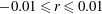 $-0.01\leqslant r\leqslant 0.01$
, a steady solution of the base flow was obtained, indicating that the forced base flow is asymptotically stable at least with respect to two-dimensional perturbations. As expected from (2.16), it is observed that a positive scale factor
$-0.01\leqslant r\leqslant 0.01$
, a steady solution of the base flow was obtained, indicating that the forced base flow is asymptotically stable at least with respect to two-dimensional perturbations. As expected from (2.16), it is observed that a positive scale factor
 $r$
increases the gain
$r$
increases the gain
 $K$
, while a negative
$K$
, while a negative
 $r$
reduces the gain. To verify the linearly predicted effects of the body force on receptivity, define an indicator
$r$
reduces the gain. To verify the linearly predicted effects of the body force on receptivity, define an indicator
 $$\begin{eqnarray}I={\rm\Delta}K/(\boldsymbol{{\rm\nabla}}_{\boldsymbol{f}}\mathscr{L},\boldsymbol{f})={\rm\Delta}K/(\boldsymbol{{\rm\nabla}}_{\boldsymbol{f}}\mathscr{L},r\boldsymbol{{\rm\nabla}}_{\boldsymbol{f}}\mathscr{L}),\end{eqnarray}$$
where
 ${\rm\Delta}K$
is the difference of the gain between using forced and unforced base flows. If
${\rm\Delta}K$
is the difference of the gain between using forced and unforced base flows. If
 $|r|$
is small enough, the body force works in the linear range and the indicator
$|r|$
is small enough, the body force works in the linear range and the indicator
 $I$
is expected to be 1. At the smallest levels of
$I$
is expected to be 1. At the smallest levels of
 $|r|$
considered, i.e.
$|r|$
considered, i.e.
 $r=10^{-5}$
, we have
$r=10^{-5}$
, we have
 $K=1.0026$
; and for increasing
$K=1.0026$
; and for increasing
 $|r|$
,
$|r|$
,
 $I$
deviates from 1 significantly as the nonlinear effects become non-negligible, as shown in figure 20(b). It can also be seen that
$I$
deviates from 1 significantly as the nonlinear effects become non-negligible, as shown in figure 20(b). It can also be seen that
 $I<1$
for negative
$I<1$
for negative
 $r$
, due to the restriction that the gain has to be positive, and therefore
$r$
, due to the restriction that the gain has to be positive, and therefore
 ${\rm\Delta}K$
has a lower bound.
${\rm\Delta}K$
has a lower bound.
Effects of the base flow modification on the distributions of the optimal inflow perturbation are revealed in figure 21. For the scale factors considered, the change in the optimal inflow perturbation is trivial, indicating that the body force acts to weaken/strengthen the existing mechanism of receptivity, but does not modify the base flow or the receptivity mechanism fundamentally. It is calculated that the relative change in the base flow, measured as
 $(\boldsymbol{U}(-0.01),\boldsymbol{U}(-0.01))/(\boldsymbol{U}(0),\boldsymbol{U}(0))$
where the base flow is considered as a function of the scale factor
$(\boldsymbol{U}(-0.01),\boldsymbol{U}(-0.01))/(\boldsymbol{U}(0),\boldsymbol{U}(0))$
where the base flow is considered as a function of the scale factor
 $r$
, is less than
$r$
, is less than
 $0.05\,\%$
.
$0.05\,\%$
.

Figure 21. Comparison of the optimal inflow perturbations
 $\tilde{\boldsymbol{u}}_{b}$
with the forced and unforced base flow at
$\tilde{\boldsymbol{u}}_{b}$
with the forced and unforced base flow at
 ${\it\tau}=150$
,
${\it\tau}=150$
,
 ${\it\omega}=0.5$
and
${\it\omega}=0.5$
and
 ${\it\beta}=0$
: (a) streamwise velocity component; (b) vertical velocity component. The magnitude is normalized so that
${\it\beta}=0$
: (a) streamwise velocity component; (b) vertical velocity component. The magnitude is normalized so that
 $[\tilde{\boldsymbol{u}}_{b},\tilde{\boldsymbol{u}}_{b}]=1$
.
$[\tilde{\boldsymbol{u}}_{b},\tilde{\boldsymbol{u}}_{b}]=1$
.
The optimal base flow modification presented in figure 19 is calculated at
 ${\it\tau}=150$
,
${\it\tau}=150$
,
 ${\it\beta}=0$
and
${\it\beta}=0$
and
 ${\it\omega}=0.5$
, and has the expected effects on receptivity at the ‘design’ parameters, as displayed in figure 20. The control effects of this modification to receptivity at out-of-design conditions are illustrated in figure 22. It is observed that the gain at the out-of-design final time and spanwise wavenumbers is also suppressed at the negative scale factor
${\it\omega}=0.5$
, and has the expected effects on receptivity at the ‘design’ parameters, as displayed in figure 20. The control effects of this modification to receptivity at out-of-design conditions are illustrated in figure 22. It is observed that the gain at the out-of-design final time and spanwise wavenumbers is also suppressed at the negative scale factor
 $r=-0.01$
. However, the receptivity at out-of-design frequencies is much less suppressed, since the optimal base flow modifications at these frequencies are dramatically different from that at
$r=-0.01$
. However, the receptivity at out-of-design frequencies is much less suppressed, since the optimal base flow modifications at these frequencies are dramatically different from that at
 ${\it\omega}=0.5$
, as has been discussed in figure 19. For the modified base flow, the maximum gain still occurs at around
${\it\omega}=0.5$
, as has been discussed in figure 19. For the modified base flow, the maximum gain still occurs at around
 ${\it\omega}=0.5$
,
${\it\omega}=0.5$
,
 ${\it\tau}=150$
and
${\it\tau}=150$
and
 ${\it\beta}=0$
, confirming that the mechanism of receptivity is weakened but not fundamentally altered. It is also worth noting that the transient effects are significantly suppressed: the contour levels become flatter with increasing
${\it\beta}=0$
, confirming that the mechanism of receptivity is weakened but not fundamentally altered. It is also worth noting that the transient effects are significantly suppressed: the contour levels become flatter with increasing
 ${\it\tau}$
, suggesting that the long-term amplification of inflow noise and the transient energy growth are highly correlated.
${\it\tau}$
, suggesting that the long-term amplification of inflow noise and the transient energy growth are highly correlated.

Figure 22. Contours of the gain
 $K$
of the modified base flow at (a)
$K$
of the modified base flow at (a)
 ${\it\beta}=0$
and (b)
${\it\beta}=0$
and (b)
 ${\it\tau}=150$
. The base flow modification is obtained at
${\it\tau}=150$
. The base flow modification is obtained at
 ${\it\tau}=150$
,
${\it\tau}=150$
,
 ${\it\beta}=0.5$
,
${\it\beta}=0.5$
,
 ${\it\omega}=0$
and
${\it\omega}=0$
and
 $r=-0.01$
.
$r=-0.01$
.
6. Correlation between amplifications of initial and boundary perturbations
In this section, the correlation between receptivity to inflow noise and receptivity to initial perturbations is explored by comparing the body forces that optimally modify amplifications of initial and boundary perturbations. The receptivity to initial perturbations and the associated transient energy growth in flow past a backward-facing step have been well studied. The optimal initial perturbation and its outcome are reproduced in the current work for further studies of base flow modifications, as shown in figure 23. As presented in § 5, the receptivity to inflow noise reaches a maximum at
 ${\it\beta}=0$
, while the receptivity to initial perturbations was reported to become maximal at
${\it\beta}=0$
, while the receptivity to initial perturbations was reported to become maximal at
 ${\it\beta}=0.645$
, with a slight increment from that at
${\it\beta}=0.645$
, with a slight increment from that at
 ${\it\beta}=0$
(Blackburn et al.
Reference Blackburn, Barkley and Sherwin2008). Therefore, to compare the mechanisms of amplification of inflow and initial perturbations, we take
${\it\beta}=0$
(Blackburn et al.
Reference Blackburn, Barkley and Sherwin2008). Therefore, to compare the mechanisms of amplification of inflow and initial perturbations, we take
 ${\it\beta}=0$
in the initial perturbation calculations.
${\it\beta}=0$
in the initial perturbation calculations.

Figure 23. Contours of spanwise vorticity in the development of the optimal initial perturbation at
 ${\it\tau}=58.1$
,
${\it\tau}=58.1$
,
 ${\it\beta}=0$
and (a)
${\it\beta}=0$
and (a)
 $t=0$
, (b)
$t=0$
, (b)
 $t=4$
, (c)
$t=4$
, (c)
 $t=20$
and (d)
$t=20$
and (d)
 $t=58.1$
. Different contour levels are chosen in each plot to highlight structures. The thick solid lines delineate the borders of recirculation bubbles.
$t=58.1$
. Different contour levels are chosen in each plot to highlight structures. The thick solid lines delineate the borders of recirculation bubbles.
The final time at which the transient energy growth of the optimal initial perturbation reaches a maximum is
 ${\it\tau}=58.1$
, which agrees well with the value reported by Blackburn et al. (Reference Blackburn, Barkley and Sherwin2008). It is seen in figure 23(a) that the optimal initial perturbation is located around the step and tilts backwards against the shear of the base flow. When this initial perturbation is convected downstream, it is compressed and amplified by the Orr mechanism (Vanneste Reference Vanneste1999; Guégan et al.
Reference Guégan, Schmid and Huerre2006), as shown in figure 23(b). Further downstream, in the region around the bubbles, the inflectional point instability manifests itself, as displayed in figure 23(c). In the region downstream of the secondary bubble, the misalignment mechanism can be observed in figure 23(d): the perturbation consists of left-headed, rectangular and right-headed structures, with the rectangular profile appearing around
${\it\tau}=58.1$
, which agrees well with the value reported by Blackburn et al. (Reference Blackburn, Barkley and Sherwin2008). It is seen in figure 23(a) that the optimal initial perturbation is located around the step and tilts backwards against the shear of the base flow. When this initial perturbation is convected downstream, it is compressed and amplified by the Orr mechanism (Vanneste Reference Vanneste1999; Guégan et al.
Reference Guégan, Schmid and Huerre2006), as shown in figure 23(b). Further downstream, in the region around the bubbles, the inflectional point instability manifests itself, as displayed in figure 23(c). In the region downstream of the secondary bubble, the misalignment mechanism can be observed in figure 23(d): the perturbation consists of left-headed, rectangular and right-headed structures, with the rectangular profile appearing around
 $x=28$
, similar to what is seen in figure 6(b). As mentioned before, the choice of contour levels in figure 23(d) shows in a clearer way that the magnitude of the perturbation grows upstream of the rectangular structure and decays downstream of it, which validates the theoretical results derived from (4.4). Therefore, the receptivities to both inflow and initial noise rely on the bubble instabilities and the misalignment mechanism for perturbation amplification. However, in the case of receptivity to inflow noise, the perturbation cannot take advantage of the Orr mechanism, since the inflow noise would be convected by the base flow to decline forwards instead of backwards.
$x=28$
, similar to what is seen in figure 6(b). As mentioned before, the choice of contour levels in figure 23(d) shows in a clearer way that the magnitude of the perturbation grows upstream of the rectangular structure and decays downstream of it, which validates the theoretical results derived from (4.4). Therefore, the receptivities to both inflow and initial noise rely on the bubble instabilities and the misalignment mechanism for perturbation amplification. However, in the case of receptivity to inflow noise, the perturbation cannot take advantage of the Orr mechanism, since the inflow noise would be convected by the base flow to decline forwards instead of backwards.
Following the procedure presented in § 2.5, the body force that optimally modifies the base flow’s amplification with respect to initial perturbations can be calculated. To illustrate the relation between the receptivities to initial and boundary perturbations, the correlation between the forces that optimally modify the amplifications of initial and boundary perturbations can be computed as
 $$\begin{eqnarray}{\it\rho}=(\boldsymbol{f}_{bp},\boldsymbol{f}_{ip})/\sqrt{(\boldsymbol{f}_{ip},\boldsymbol{ f}_{ip})(\boldsymbol{f}_{bp},\boldsymbol{ f}_{bp})},\end{eqnarray}$$
where
 $\boldsymbol{f}_{bp}$
refers to the body force that optimally modifies amplifications of boundary perturbations (inflow noise) at a large enough final time
$\boldsymbol{f}_{bp}$
refers to the body force that optimally modifies amplifications of boundary perturbations (inflow noise) at a large enough final time
 ${\it\tau}=150$
, so as to eliminate transient energy growth, and
${\it\tau}=150$
, so as to eliminate transient energy growth, and
 $\boldsymbol{f}_{ip}$
is the body force that optimally modifies amplifications of initial perturbations at
$\boldsymbol{f}_{ip}$
is the body force that optimally modifies amplifications of initial perturbations at
 ${\it\tau}=58.1$
, at which the transient growth is maximized over the parameters considered.
${\it\tau}=58.1$
, at which the transient growth is maximized over the parameters considered.
As revealed in figure 24, the correlation
 ${\it\rho}$
is approximately zero at
${\it\rho}$
is approximately zero at
 ${\it\omega}=0$
, indicating that the receptivities to steady inflow noise and the optimal initial perturbation are almost decoupled. At
${\it\omega}=0$
, indicating that the receptivities to steady inflow noise and the optimal initial perturbation are almost decoupled. At
 ${\it\omega}\approx 0.5$
, where the receptivity to inflow noise attains a maximum, the correlation between the receptivities to inflow and initial perturbations also becomes maximal and reaches 0.973, indicating that the two body forces almost overlap. This observation suggests that the most dramatic amplifications of inflow perturbations and initial perturbations rely on the same mechanisms (the bubble instabilities and the misalignment mechanism) and can be controlled simultaneously by a body force. Also notice that as
${\it\omega}\approx 0.5$
, where the receptivity to inflow noise attains a maximum, the correlation between the receptivities to inflow and initial perturbations also becomes maximal and reaches 0.973, indicating that the two body forces almost overlap. This observation suggests that the most dramatic amplifications of inflow perturbations and initial perturbations rely on the same mechanisms (the bubble instabilities and the misalignment mechanism) and can be controlled simultaneously by a body force. Also notice that as
 ${\it\omega}$
becomes larger, this correlation drops, in agreement with the previous discussion that the receptivity to inflow noise at high frequencies depends on the primary bubble instability, and the misalignment mechanism downstream of the secondary bubble is almost irrelevant.
${\it\omega}$
becomes larger, this correlation drops, in agreement with the previous discussion that the receptivity to inflow noise at high frequencies depends on the primary bubble instability, and the misalignment mechanism downstream of the secondary bubble is almost irrelevant.

Figure 24. Correlation between the body force that optimally modifies amplifications of inflow noise at
 ${\it\beta}=0$
and
${\it\beta}=0$
and
 ${\it\tau}=150$
and the body force that optimally modifies amplifications of the initial perturbation at
${\it\tau}=150$
and the body force that optimally modifies amplifications of the initial perturbation at
 ${\it\beta}=0$
and
${\it\beta}=0$
and
 ${\it\tau}=58.1$
, plotted for various frequencies
${\it\tau}=58.1$
, plotted for various frequencies
 ${\it\omega}$
.
${\it\omega}$
.
It is worth mentioning that there is another, more intuitive way of illustrating the correlation between receptivities to boundary and initial perturbations, i.e. to compare the outcomes of the optimal initial perturbation and the optimal inflow perturbation. However, as can be seen in figure 6(b), the outcome of the optimal boundary perturbation spreads over the region downstream of the step, while, as shown in figure 23(d), the outcome of the optimal initial perturbation is located downstream of the bubbles and the contribution of the bubble instabilities to the energy growth is not directly evident because of the convection effects. Therefore the profile of the perturbation outcome does not cover all the amplification mechanisms, and the correlation between the outcomes of the initial and boundary perturbations is physically less meaningful than the correlation of the optimal body forces.
The receptivity to initial perturbations, measured by the transient energy growth
 $G$
, which is calculated using the unforced and optimally forced base flow, is shown in figure 25. It is seen that at a scale factor of
$G$
, which is calculated using the unforced and optimally forced base flow, is shown in figure 25. It is seen that at a scale factor of
 $|r|=10^{-5}$
, the maximum transient growth can be enhanced or suppressed by an order of magnitude. As the transient growth is suppressed (respectively, enhanced), the optimal final time decreases (respectively, increases), because in the modified flow the rectangular streamlines appear earlier (respectively, later), further confirming the role of the misalignment mechanism in noise amplification.
$|r|=10^{-5}$
, the maximum transient growth can be enhanced or suppressed by an order of magnitude. As the transient growth is suppressed (respectively, enhanced), the optimal final time decreases (respectively, increases), because in the modified flow the rectangular streamlines appear earlier (respectively, later), further confirming the role of the misalignment mechanism in noise amplification.

Figure 25. Transient growth of the controlled and uncontrolled flow at
 ${\it\beta}=0$
. The maximum growth point on each curve is highlighted by dotted lines.
${\it\beta}=0$
. The maximum growth point on each curve is highlighted by dotted lines.
7. Conclusion
Noise amplification of the flow past a backward-facing step with an expansion ratio of 0.5 is investigated. As in previous work by Blackburn et al. (Reference Blackburn, Barkley and Sherwin2008), in most of this work the Reynolds number is fixed at
 $\mathit{Re}=500$
, at which the unperturbed base flow is steady and two-dimensional, featuring a primary bubble attached to the lower wall and a secondary bubble attached to the upper wall. Depending on the source of the perturbations, the amplification effects can be classified into receptivity to initial perturbations and receptivity to inflow boundary perturbations.
$\mathit{Re}=500$
, at which the unperturbed base flow is steady and two-dimensional, featuring a primary bubble attached to the lower wall and a secondary bubble attached to the upper wall. Depending on the source of the perturbations, the amplification effects can be classified into receptivity to initial perturbations and receptivity to inflow boundary perturbations.
Since the receptivity to initial perturbations (transient growth of the initial perturbation) in flow past a backward-facing step has been well studied, the present work focuses on the receptivity to inflow noise. A large enough final time
 ${\it\tau}=150$
is used to isolate the receptivity from transient energy growth. It is found that the receptivity to inflow noise is maximized at spanwise wavenumber
${\it\tau}=150$
is used to isolate the receptivity from transient energy growth. It is found that the receptivity to inflow noise is maximized at spanwise wavenumber
 ${\it\beta}=0$
and frequency
${\it\beta}=0$
and frequency
 ${\it\omega}=0.5$
, at which the magnitude of the inflow velocity perturbation is amplified over two orders of magnitude. The receptivity can be explained by a combination of bubble-induced inflectional point instabilities and a misalignment mechanism, which transfers perturbations downstream of the secondary bubble to left-headed, rectangular and right-headed structures. The magnitude of the perturbation grows in the left-headed region until it reaches the rectangular profile, downstream of which, in the right-headed region, the magnitude decays. In the region further downstream, the base flow stretches the perturbation and the structure becomes more sharply right-headed. Therefore the perturbation growth induced by the misalignment mechanism is self-limiting. The most amplified inflow perturbation, i.e. the one with
${\it\omega}=0.5$
, at which the magnitude of the inflow velocity perturbation is amplified over two orders of magnitude. The receptivity can be explained by a combination of bubble-induced inflectional point instabilities and a misalignment mechanism, which transfers perturbations downstream of the secondary bubble to left-headed, rectangular and right-headed structures. The magnitude of the perturbation grows in the left-headed region until it reaches the rectangular profile, downstream of which, in the right-headed region, the magnitude decays. In the region further downstream, the base flow stretches the perturbation and the structure becomes more sharply right-headed. Therefore the perturbation growth induced by the misalignment mechanism is self-limiting. The most amplified inflow perturbation, i.e. the one with
 ${\it\omega}=0.5$
, takes full advantage of the bubble instabilities and misalignment mechanisms, whereas perturbations of higher or lower frequencies are amplified only around the primary bubble and the fore segment of the secondary bubble. Similar optimal frequency and receptivity mechanisms are observed at higher Reynolds numbers, up to
${\it\omega}=0.5$
, takes full advantage of the bubble instabilities and misalignment mechanisms, whereas perturbations of higher or lower frequencies are amplified only around the primary bubble and the fore segment of the secondary bubble. Similar optimal frequency and receptivity mechanisms are observed at higher Reynolds numbers, up to
 $\mathit{Re}=1000$
.
$\mathit{Re}=1000$
.
The nonlinear development of the optimal boundary perturbation is studied through DNS. It is observed that at low magnitudes of inflow perturbations, vortex shedding occurs downstream of the secondary bubble. As the magnitude of perturbations increases, flapping of the separation and reattachment points of the bubbles is observed, and smaller bubbles are induced along the wall. When the maximum inflow perturbation reaches 1.4 % of the free-stream velocity, the flow becomes three-dimensional. It is also observed that the three-dimensional and turbulent developments of the perturbed flow enhance mixing and significantly reduce the size of the recirculation zones. The Strouhal number of bubble flapping in the flow perturbed by both optimal and random inflow noise is 0.08, which agrees with the frequency of the globally optimal inflow perturbation. This Strouhal number has been reported to be 0.06 (Le et al.
Reference Le, Moin and Kim1997), 0.07 (Métais Reference Métais2001), 0.05–0.1 (Kaiktsis et al.
Reference Kaiktsis, Karniadakis and Orszag1996) and
 $O(0.1)$
(Wee et al.
Reference Wee, Yi, Annaswamy and Ghoniem2004) at larger Reynolds numbers or in fully turbulent regimes. Even though these previous results were obtained at larger Reynolds numbers, the close agreement with the current work suggests that bubble flapping can be a consequence of receptivity to inflow noise.
$O(0.1)$
(Wee et al.
Reference Wee, Yi, Annaswamy and Ghoniem2004) at larger Reynolds numbers or in fully turbulent regimes. Even though these previous results were obtained at larger Reynolds numbers, the close agreement with the current work suggests that bubble flapping can be a consequence of receptivity to inflow noise.
Further investigations of base flow modifications are conducted to reveal the mechanism of noise amplification and to explore the control of receptivities. To preserve the divergence-free condition, the base flow is modified by a body force. It is worth noting that boundary suction/blowing can be physically more useful for modifying or controlling the base flow, but the body force is more effective in changing the flow even in regions far from boundaries, and therefore it is a suitable tool for studying the mechanisms of noise amplification. A numerical method is developed to calculate the linearly optimal body force; this method accommodates both initial and boundary perturbation problems. The distribution of the base flow modification due to the linearly optimal body force is found to be strongly correlated with the outcome of the inflow noise. At
 ${\it\omega}=0.5$
, the modification is located around the bubbles and the shear layers downstream of the bubble, which modifies the bubble-induced instabilities and the misalignment mechanism. At lower and higher frequencies, the modification concentrates around the primary bubble and the fore part of the secondary bubble, reflecting the irrelevance in these cases of the misalignment mechanism in the region downstream of the secondary bubble. However, the distribution of the optimal inflow perturbation is insensitive to the base flow modifications, indicating that the modifications do not alter the fundamental features of the flow. A modification with a relative energy change of 0.05 % is found to reduce the maximum receptivity by around two orders of magnitude. The modification effects on receptivity are preserved for out-of-design final times and spanwise wavenumbers, but do not work well for out-of-design noise frequencies, owing to the variation of mechanisms at different frequencies.
${\it\omega}=0.5$
, the modification is located around the bubbles and the shear layers downstream of the bubble, which modifies the bubble-induced instabilities and the misalignment mechanism. At lower and higher frequencies, the modification concentrates around the primary bubble and the fore part of the secondary bubble, reflecting the irrelevance in these cases of the misalignment mechanism in the region downstream of the secondary bubble. However, the distribution of the optimal inflow perturbation is insensitive to the base flow modifications, indicating that the modifications do not alter the fundamental features of the flow. A modification with a relative energy change of 0.05 % is found to reduce the maximum receptivity by around two orders of magnitude. The modification effects on receptivity are preserved for out-of-design final times and spanwise wavenumbers, but do not work well for out-of-design noise frequencies, owing to the variation of mechanisms at different frequencies.
In optimal initial perturbation studies, it is confirmed that the transient energy growth of the initial perturbation also stems from the bubble instability and the misalignment mechanism. From the correlation between the body forces that optimally modify receptivities to inflow and initial perturbations, it is found that the base flow modification that suppresses receptivity to initial perturbations also suppresses receptivity to inflow perturbations at the most amplified frequency. However, at higher or lower frequencies, the correlation drops, confirming that high- and low-frequency receptivity to inflow noise relies on different mechanisms than the transient energy growth of initial perturbations. The base flow modification study also suggests that the optimal body force or optimal modification can reveal the complete mechanisms of noise amplification, which cannot be fully identified from the outcome of the optimal initial or boundary perturbations.
Acknowledgements
The author would like to thank Dr L. Lesshafft and Professor P. Schmid for helpful discussions, and acknowledges the support of a postdoctoral fellowship from the EADS Foundation when starting this work in LadHyX, École Polytechnique. This work made use of the facilities of N8 HPC provided and funded by the N8 consortium and EPSRC (grant no. EP/K000225/1). The Centre is coordinated by the Universities of Leeds and Manchester.
Appendix A. Lagrangian functional
Similar to (2.10), a ‘symmetric’ Lagrangian functional can be defined as
 $$\begin{eqnarray}\displaystyle \mathscr{L} & = & \displaystyle K+\langle {\bf\lambda}_{1},\partial _{t}\boldsymbol{u}-L(\boldsymbol{U})\boldsymbol{u}\rangle +\langle {\bf\lambda}_{2},\partial _{t}\boldsymbol{u}^{\ast }+L^{\ast }(\boldsymbol{U})\boldsymbol{u}^{\ast }\rangle \nonumber\\ \displaystyle & & \displaystyle +\,[{\bf\lambda}_{3},\boldsymbol{g}(\boldsymbol{u}^{\ast })-K\tilde{\boldsymbol{u}}_{b}]+({\bf\lambda}_{4},\boldsymbol{u}({\it\tau})-\boldsymbol{u}^{\ast }({\it\tau}))+({\bf\lambda}_{5},D\boldsymbol{U}-\boldsymbol{f}),\end{eqnarray}$$
where the
 ${\bf\lambda}_{i}$
(
${\bf\lambda}_{i}$
(
 $1\leqslant i\leqslant 5$
) are Lagrange multipliers:
$1\leqslant i\leqslant 5$
) are Lagrange multipliers:
 ${\bf\lambda}_{1}$
and
${\bf\lambda}_{1}$
and
 ${\bf\lambda}_{2}$
are time-dependent variables defined on the domain
${\bf\lambda}_{2}$
are time-dependent variables defined on the domain
 ${\it\Omega}$
and time interval
${\it\Omega}$
and time interval
 $[0,{\it\tau}]$
,
$[0,{\it\tau}]$
,
 ${\bf\lambda}_{3}$
is a time-independent variable defined on the perturbation boundary
${\bf\lambda}_{3}$
is a time-independent variable defined on the perturbation boundary
 $\partial {\it\Omega}_{b}$
, and
$\partial {\it\Omega}_{b}$
, and
 ${\bf\lambda}_{4}$
and
${\bf\lambda}_{4}$
and
 ${\bf\lambda}_{5}$
are time-independent variables on
${\bf\lambda}_{5}$
are time-independent variables on
 ${\it\Omega}$
. The first term on the right-hand side is the optimal gain over all possible boundary perturbations; the second, third, fourth and fifth terms constitute the constraint that
${\it\Omega}$
. The first term on the right-hand side is the optimal gain over all possible boundary perturbations; the second, third, fourth and fifth terms constitute the constraint that
 $\tilde{\boldsymbol{u}}_{b}$
is the optimal boundary perturbation; and the final term is the constraint specifying that the base flow
$\tilde{\boldsymbol{u}}_{b}$
is the optimal boundary perturbation; and the final term is the constraint specifying that the base flow
 $\boldsymbol{U}$
is a steady solution of the forced NS equations (2.2).
$\boldsymbol{U}$
is a steady solution of the forced NS equations (2.2).
One may integrate the second and third terms in (A 1) by parts to obtain
 $$\begin{eqnarray}\displaystyle \mathscr{L} & = & \displaystyle K-\langle \boldsymbol{u},\partial _{t}{\bf\lambda}_{1}+L^{\ast }(\boldsymbol{U}){\bf\lambda}_{1}\rangle +(\boldsymbol{u}({\it\tau}),{\bf\lambda}_{1}({\it\tau}))-[\boldsymbol{g}({\bf\lambda}_{1}),\tilde{\boldsymbol{u}}_{b}]-\langle \boldsymbol{u}^{\ast },\partial _{t}{\bf\lambda}_{2}-L(\boldsymbol{U}){\bf\lambda}_{2}\rangle \nonumber\\ \displaystyle & & \displaystyle +\,(\boldsymbol{u}^{\ast }({\it\tau}),{\bf\lambda}_{2}({\it\tau}))-[\boldsymbol{g}(\boldsymbol{u}^{\ast }),{\bf\lambda}_{2b}]+[{\bf\lambda}_{3},\boldsymbol{g}(\boldsymbol{u}^{\ast })-K\tilde{\boldsymbol{u}}_{b}]\nonumber\\ \displaystyle & & \displaystyle +\,({\bf\lambda}_{4},\boldsymbol{u}({\it\tau})-\boldsymbol{u}^{\ast }({\it\tau}))+({\bf\lambda}_{5},D\boldsymbol{U}-\boldsymbol{f}),\end{eqnarray}$$
where
 ${\bf\lambda}_{2b}$
is defined on the perturbation boundary and satisfies
${\bf\lambda}_{2b}$
is defined on the perturbation boundary and satisfies
 ${\bf\lambda}_{2}({\it\tau})=\mathscr{M}({\it\tau}){\bf\lambda}_{2b}$
, with
${\bf\lambda}_{2}({\it\tau})=\mathscr{M}({\it\tau}){\bf\lambda}_{2b}$
, with
 $\mathscr{M}({\it\tau})$
being an operator that evolves a boundary perturbation to a final outcome, whose action corresponds to integration of the linearized NS equations.
$\mathscr{M}({\it\tau})$
being an operator that evolves a boundary perturbation to a final outcome, whose action corresponds to integration of the linearized NS equations.
Setting to zero the first variations of
 $\mathscr{L}$
with respect to
$\mathscr{L}$
with respect to
 ${\bf\lambda}_{i}$
(
${\bf\lambda}_{i}$
(
 $1\leqslant i\leqslant 5$
) recovers the constraint that
$1\leqslant i\leqslant 5$
) recovers the constraint that
 $\tilde{\boldsymbol{u}}_{b}$
is the optimal boundary perturbation leading to the largest gain
$\tilde{\boldsymbol{u}}_{b}$
is the optimal boundary perturbation leading to the largest gain
 $K$
to the base flow
$K$
to the base flow
 $\boldsymbol{U}$
, which is a steady solution of the NS equations (2.2). Setting to zero the first variations of
$\boldsymbol{U}$
, which is a steady solution of the NS equations (2.2). Setting to zero the first variations of
 $\mathscr{L}$
with respect to
$\mathscr{L}$
with respect to
 $\boldsymbol{u}^{\ast }({\it\tau})$
,
$\boldsymbol{u}^{\ast }({\it\tau})$
,
 $\boldsymbol{u}({\it\tau})$
,
$\boldsymbol{u}({\it\tau})$
,
 $\tilde{\boldsymbol{u}}_{b}$
,
$\tilde{\boldsymbol{u}}_{b}$
,
 $\boldsymbol{g}(\boldsymbol{u}^{\ast })$
and
$\boldsymbol{g}(\boldsymbol{u}^{\ast })$
and
 $K$
, we obtain the following equations:
$K$
, we obtain the following equations:
 $$\begin{eqnarray}\displaystyle \displaystyle \frac{{\it\delta}\mathscr{L}}{{\it\delta}\boldsymbol{u}^{\ast }({\it\tau})}=0\quad & \Rightarrow & \displaystyle \quad {\bf\lambda}_{2}({\it\tau})={\bf\lambda}_{4},\end{eqnarray}$$
 $$\begin{eqnarray}\displaystyle \displaystyle \frac{{\it\delta}\mathscr{L}}{{\it\delta}\boldsymbol{u}({\it\tau})}=0\quad & \Rightarrow & \displaystyle \quad {\bf\lambda}_{1}({\it\tau})=-{\bf\lambda}_{4},\end{eqnarray}$$
 $$\begin{eqnarray}\displaystyle \displaystyle \frac{{\it\delta}\mathscr{L}}{{\it\delta}\tilde{\boldsymbol{u}}_{b}}=0\quad & \Rightarrow & \displaystyle \quad -\boldsymbol{g}({\bf\lambda}_{1})=K{\bf\lambda}_{3},\end{eqnarray}$$
 $$\begin{eqnarray}\displaystyle \displaystyle \frac{{\it\delta}\mathscr{L}}{{\it\delta}\boldsymbol{g}(\boldsymbol{u}^{\ast })}=0\quad & \Rightarrow & \displaystyle \quad {\bf\lambda}_{2b}={\bf\lambda}_{3},\end{eqnarray}$$
 $$\begin{eqnarray}\displaystyle \displaystyle \frac{{\it\delta}\mathscr{L}}{{\it\delta}K}=0\quad & \Rightarrow & \displaystyle \quad [{\bf\lambda}_{3},\tilde{\boldsymbol{u}}_{b}]=1.\end{eqnarray}$$
 ${\bf\lambda}_{3}$
and
${\bf\lambda}_{3}$
and
 ${\bf\lambda}_{4}$
, we have
${\bf\lambda}_{4}$
, we have  $$\begin{eqnarray}[{\bf\lambda}_{2b},\tilde{\boldsymbol{u}}_{b}]=1,\quad -\boldsymbol{g}({\bf\lambda}_{1})=K{\bf\lambda}_{2b}\quad \text{and}\quad {\bf\lambda}_{1}({\it\tau})=-{\bf\lambda}_{2}({\it\tau}).\end{eqnarray}$$
Substituting into (A 8) the operator
 $\mathscr{M}$
and its adjoint
$\mathscr{M}$
and its adjoint
 $\mathscr{M}^{\ast }$
, whose action corresponds to integration of the adjoint equation, yields
$\mathscr{M}^{\ast }$
, whose action corresponds to integration of the adjoint equation, yields
 $$\begin{eqnarray}\mathscr{M}^{\ast }({\it\tau})\mathscr{M}({\it\tau}){\bf\lambda}_{2b}=K{\bf\lambda}_{2b}.\end{eqnarray}$$
Clearly,
 ${\bf\lambda}_{2b}$
is the eigenvector of the joint operator
${\bf\lambda}_{2b}$
is the eigenvector of the joint operator
 $\mathscr{M}^{\ast }({\it\tau})\mathscr{M}({\it\tau})$
corresponding to the largest eigenvalue
$\mathscr{M}^{\ast }({\it\tau})\mathscr{M}({\it\tau})$
corresponding to the largest eigenvalue
 $K$
. Therefore
$K$
. Therefore
 ${\bf\lambda}_{2b}$
is parallel to
${\bf\lambda}_{2b}$
is parallel to
 $\tilde{\boldsymbol{u}}_{b}$
. By standard algebraic manipulations, one obtains
$\tilde{\boldsymbol{u}}_{b}$
. By standard algebraic manipulations, one obtains
 $$\begin{eqnarray}{\bf\lambda}_{2b}=\tilde{\boldsymbol{u}}_{b}/[\tilde{\boldsymbol{u}}_{b},\tilde{\boldsymbol{u}}_{b}],\quad {\bf\lambda}_{2}({\it\tau})=\boldsymbol{u}({\it\tau})/[\tilde{\boldsymbol{u}}_{b},\tilde{\boldsymbol{u}}_{b}]\quad \text{and}\quad {\bf\lambda}_{1}({\it\tau})=-\boldsymbol{u}^{\ast }({\it\tau})/[\tilde{\boldsymbol{u}}_{b},\tilde{\boldsymbol{u}}_{b}],\end{eqnarray}$$
and hence
 $$\begin{eqnarray}{\bf\lambda}_{1}=-\boldsymbol{u}^{\ast }/[\tilde{\boldsymbol{u}}_{b},\tilde{\boldsymbol{u}}_{b}]\quad \text{and}\quad {\bf\lambda}_{2}=\boldsymbol{u}/[\tilde{\boldsymbol{u}}_{b},\tilde{\boldsymbol{u}}_{b}].\end{eqnarray}$$
In (A 1), the variation of the second and third terms on the right-hand side with respect to the base flow
 $\boldsymbol{U}$
can be formulated as
$\boldsymbol{U}$
can be formulated as
 $$\begin{eqnarray}\displaystyle & & \displaystyle {\it\delta}\langle {\bf\lambda}_{1},\partial _{t}\boldsymbol{u}-L(\boldsymbol{U})\boldsymbol{u}\rangle +{\it\delta}\langle {\bf\lambda}_{2},\partial _{t}\boldsymbol{u}^{\ast }+L^{\ast }(\boldsymbol{U})\boldsymbol{u}^{\ast }\rangle \nonumber\\ \displaystyle & & \displaystyle \quad =\langle {\it\delta}\boldsymbol{U},\boldsymbol{{\rm\nabla}}\boldsymbol{u}\boldsymbol{\cdot }{\bf\lambda}_{1}\rangle -\langle {\it\delta}\boldsymbol{U},\boldsymbol{u}\boldsymbol{\cdot }\boldsymbol{{\rm\nabla}}{\bf\lambda}_{1}\rangle +\langle {\it\delta}\boldsymbol{U},\boldsymbol{{\rm\nabla}}\boldsymbol{u}^{\ast }\boldsymbol{\cdot }{\bf\lambda}_{2}\rangle +\langle {\it\delta}\boldsymbol{U},{\bf\lambda}_{2}\boldsymbol{\cdot }\boldsymbol{{\rm\nabla}}\boldsymbol{u}^{\ast }\rangle .\end{eqnarray}$$
In deriving this equation, (A 11) has been used to eliminate the terms involving surface integrations over the outflow boundary. Similarly, the variation of the last term with respect to the base flow
 $\boldsymbol{U}$
can be written as
$\boldsymbol{U}$
can be written as
 $$\begin{eqnarray}{\it\delta}({\bf\lambda}_{5},D\boldsymbol{U}-\boldsymbol{f})({\it\delta}\boldsymbol{U})=-({\it\delta}\boldsymbol{U},L^{\ast }(\boldsymbol{U}){\bf\lambda}_{5}).\end{eqnarray}$$
By combining (A 12) and (A 13), the variation of the Lagrangian functional with respect to the base flow can be obtained:
 $$\begin{eqnarray}{\it\delta}\mathscr{L}({\it\delta}\boldsymbol{U})=({\it\delta}\boldsymbol{U},\boldsymbol{F}_{s}-L^{\ast }(\boldsymbol{U}){\bf\lambda}_{5}),\end{eqnarray}$$
where
 $$\begin{eqnarray}\boldsymbol{F}_{s}={\it\tau}^{-1}\int _{0}^{{\it\tau}}(\boldsymbol{{\rm\nabla}}\boldsymbol{u}\boldsymbol{\cdot }{\bf\lambda}_{1}-\boldsymbol{u}\boldsymbol{\cdot }\boldsymbol{{\rm\nabla}}{\bf\lambda}_{1}+\boldsymbol{{\rm\nabla}}\boldsymbol{u}^{\ast }\boldsymbol{\cdot }{\bf\lambda}_{2}+{\bf\lambda}_{2}\boldsymbol{\cdot }\boldsymbol{{\rm\nabla}}\boldsymbol{u}^{\ast })\,\text{d}t\end{eqnarray}$$
denotes the gradient of the Lagrangian functional with respect to the base flow, without the constraint that the base flow satisfies the NS equations (the last term in (A 1)). Substituting (A 11) into (A 15) gives
 $$\begin{eqnarray}\boldsymbol{F}_{s}={\it\tau}^{-1}\int _{0}^{{\it\tau}}(-\boldsymbol{{\rm\nabla}}\boldsymbol{u}\boldsymbol{\cdot }\boldsymbol{u}^{\ast }+2\boldsymbol{u}\boldsymbol{\cdot }\boldsymbol{{\rm\nabla}}\boldsymbol{u}^{\ast }+\boldsymbol{{\rm\nabla}}\boldsymbol{u}^{\ast }\boldsymbol{\cdot }\boldsymbol{u})\,\text{d}t/[\tilde{\boldsymbol{u}}_{b},\tilde{\boldsymbol{u}}_{b}].\end{eqnarray}$$
Owing to the form of the Lagrangian functional, no further assumptions are introduced in the derivation of (A 16). Therefore the assumption that the base flow variation is zero on the boundaries, as used in (2.18), can be released. Replacing
 $\boldsymbol{F}$
in (2.19) by
$\boldsymbol{F}$
in (2.19) by
 $\boldsymbol{F}_{s}$
and following the procedures in § 2.5, the same results for the linearly optimal body force can be obtained.
$\boldsymbol{F}_{s}$
and following the procedures in § 2.5, the same results for the linearly optimal body force can be obtained.


