


1. Introduction
Studies on internal tides (ITs) have attracted considerable attention over the years, because these waves can have a significant impact on oceanic mixing (Munk & Wunsch Reference Munk and Wunsch1998; Vic et al. Reference Vic, Garabato, Green, Waterhouse, Zhao, Melet, De Lavergne, Buijsman and Stephenson2019), large scale ocean circulation (Wunsch & Ferrari Reference Wunsch and Ferrari2004), transport of energy (Simmons & Alford Reference Simmons and Alford2012), upwelling of nutrients (Schafstall et al. Reference Schafstall, Dengler, Brandt and Bange2010) and shaping the continental shelves (Cacchione, Pratson & Ogston Reference Cacchione, Pratson and Ogston2002). In situ observations suggest that strong mixing occurs over rough bathymetry (Polzin et al. Reference Polzin, Toole, Ledwell and Schmitt1997), the biweekly variation of the mixing indicating a relationship to the spring-neap barotropic tidal cycle and thus to the conversion of barotropic to baroclinic tidal energy. The most prominent IT generation mechanism is barotropic tidal flows incident upon bottom topography such as the continental shelf slope, subsurface ridges and seamounts. Examples of generation locations include the Bay of Biscay (New & Pingree Reference New and Pingree1992; Gerkema, Lam & Maas Reference Gerkema, Lam and Maas2004), the Australian North West Shelf (Holloway, Chatwin & Craig Reference Holloway, Chatwin and Craig2001), the Malin–Hebrides Shelf (Xing & Davies Reference Xing and Davies1998), the Hawaiian Ridge (Martin, Rudnick & Pinkel Reference Martin, Rudnick and Pinkel2006), Mid-Atlantic Ridge (Zilberman et al. Reference Zilberman, Becker, Merrifield and Carter2009), Monterey Bay (Lien & Gregg Reference Lien and Gregg2001) and various seamounts (Lueck & Mudge Reference Lueck and Mudge1997; Toole et al. Reference Toole, Schmitt, Polzin and Kunze1997). Global numerical simulations (Simmons, Hallberg & Arbic Reference Simmons, Hallberg and Arbic2004; Niwa & Hibiya Reference Niwa and Hibiya2011) have been conducted to investigate the spatial distribution of the major generation sites. They found that the generation of baroclinic tides largely occurs over prominent topographic features and the total conversion rate increases as the model grid spacing is reduced.
There are three important dimensionless parameters relevant to internal waves (IWs) generated by tide–topography interaction. The first one is the tidal excursion parameter  $\epsilon$, which is used to measure the nonlinearity of the waves (Vlasenko, Stashchuk & Hutter Reference Vlasenko, Stashchuk and Hutter2005; Legg & Huijts Reference Legg and Huijts2006; Garrett & Kunze Reference Garrett and Kunze2007). It is defined as the ratio of the barotropic tidal advection distance to the horizontal scale of the topography. If
  $\epsilon$ is much smaller than 1, linear ITs are generated mainly at the forcing frequency. The second dimensionless parameter is the relative height of the topography
  $\delta = h/H$, where
  $h$ is the topographic height and
  $H$ is a typical water depth. The third important parameter for IT generation is the bottom slope criticality
  $\alpha = s/\gamma$, where
  $s$ is the topographic slope and
  $\gamma$ is the slope of an IT characteristic. In the presence of a barotropic background flow
  $V(x)$ in the
  $y$-direction, which varies slowly in the
  $x$-direction so that second-order gradients are negligible, under the hydrostatic approximation,
 \begin{equation} \gamma = \sqrt{ \frac{\sigma_T^{2} - f_{eff}^{2}}{N^{2}} }. \end{equation}
Here  $f_{eff}^{2} = f^{2} + f\kern0.06em V_x$ is the effective Coriolis frequency squared (Mooers Reference Mooers1975),
  $\sigma _T$ is the IT frequency and
  $N$ is the buoyancy frequency. In general,
  $N$ is a function of
  $z$ and
  $\gamma$ can depend on both
  $x$ and
  $z$.
$z$.
The critical latitude is defined as the latitude where  $f = \sigma _T$ for each tidal constituent. Critical latitudes are approximately 30
 $^{\circ }$ and 75
 $^{\circ }$ for the diurnal
  $K_1$ and semi-diurnal
  $M_2$ tides, respectively. Note that (1.1) is not valid if
  $f_{eff} > \sigma _T$. Instead we have an evanescent region, where no freely propagating waves are permitted and forced waves decay quasi-exponentially away from the generation site. If the length of the evanescent region is finite, meaning
  $f_{eff}$ varies spatially, a fraction of the wave energy can tunnel through the region and there is a radiated wave on the other side of the region. Intensive research on tunnelling has been done with most of it focused on vertically propagating waves in the atmospheric context (Jones Reference Jones1970; Monserrat & Thorpe Reference Monserrat and Thorpe1996; Sutherland & Yewchuk Reference Sutherland and Yewchuk2004), though some work has discussed tunnelling in the ocean (Eckart Reference Eckart1961; Rainville & Pinkel Reference Rainville and Pinkel2004).
Unlike numerical studies, the theoretical models all use linearized equations of motion and most of them are formulated without a background current, i.e.  $f_{eff}=f$. When
  $\alpha$ is much less than 1, the analysis of Bell (Reference Bell1975) has been widely used for small amplitude bathymetry
  $\delta \ll 1$. Bell included the advection by the background flow and used an infinitely deep ocean to estimate the upward energy flux for subcritical topography to be
  $O(1)$ mW m
 $^{-2}$. Building upon Bell's work, Khatiwala (Reference Khatiwala2003) included a rigid lid, which results in horizontal, rather than vertical, energy flux. He found good agreement with that predicted by a nonlinear numerical model. Llewellyn Smith & Young (Reference Llewellyn Smith and Young2002) too present an analytical treatment of this problem by using a different mathematical approach (WKB method) to include non-uniform
  $N(z)$. While most models with small bathymetry
  $\delta \ll 1$ use a linearized bottom boundary condition, St. Laurent & Garrett (Reference St. Laurent and Garrett2002) used a perturbation expansion of the bottom boundary condition for small but finite amplitude topography. However, the linear theory in general underestimates the energy flux for supercritical cases.
Bathymetries with large amplitudes have also been considered theoretically. In this case, the bottom boundary condition cannot be linearized. For subcritical slopes with  $\alpha < 1$, the model developed by Baines (Reference Baines1982) is available. Craig (Reference Craig1987) used the method of characteristics and described the generation of ITs of a single frequency at shelf-like topography with a constant shelf slope. He found that energy flux varies linearly with
  $\alpha$ and like
  $\alpha ^{5}$ for supercritical and subcritical cases, respectively. Similar results for subcritical cases were obtained by Vlasenko et al. (Reference Vlasenko, Stashchuk and Hutter2005). Balmforth, Ierley & Young (Reference Balmforth, Ierley and Young2002) considered an infinitely deep ocean, while a finite depth ocean was discussed by St. Laurent et al. (Reference St. Laurent, Stringer, Garrett and Perrault-Joncas2003) with a finite amplitude knife edge, step-like and top hat bathymetry. This work was extended by Nycander (Reference Nycander2006), where he considered periodic knife edge bathymetry. Pétrélis, Smith & Young (Reference Pétrélis, Smith and Young2006) applied a Green's function to large submarine ridges assuming small tidal excursion distance
  $\epsilon$. Their results confirm a monotonic increase in the radiated energy flux as the slope becomes steeper, with most of the increase happening after the slope becomes slightly supercritical. Other models include those of Gerkema (Reference Gerkema2002), Gerkema et al. (Reference Gerkema, Lam and Maas2004) and Baines (Reference Baines1973). However, none of these models on large amplitude bathymetries include advection by the barotropic tide and they generally need to be solved numerically owing to the model complexity. Therefore, they are restricted to small tidal excursions.
Numerical simulations using primitive equation models to study IT generation by tide–topography interaction have become increasingly important particularly for regions where linear theories break down or become complex. Legg & Huijts (Reference Legg and Huijts2006) used a Gaussian ridge to confirm that strong local mixing only occurs for narrow features with large  $\alpha$, which is common in the coastal ocean. Holloway & Merrifield (Reference Holloway and Merrifield1999) and Munroe & Lamb (Reference Munroe and Lamb2005) focused on idealized seamounts and showed that large seamounts are ineffective at generating ITs unless they are elongated in a direction normal to the barotropic tides. The aforementioned papers all used free surface in their models, while Lamb & Kim (Reference Lamb and Kim2012) applied a rigid lid and concluded that the large amplitude theory yields good results with simulations using subcritical slopes. Investigations of IT generation using more realistic bathymetries are numerous, e.g. Powell et al. (Reference Powell, Janeković, Carter and Merrifield2012), Niwa & Hibiya (Reference Niwa and Hibiya2004, Reference Niwa and Hibiya2014), Merrifield, Holloway & Johnston (Reference Merrifield, Holloway and Johnston2001), Holloway (Reference Holloway1996) and Zilberman et al. (Reference Zilberman, Becker, Merrifield and Carter2009). More details on the theories and numerical simulations can be found in the review by Garrett & Kunze (Reference Garrett and Kunze2007).
Most of the aforementioned research is relatively basic in the sense that only the effect of barotropic tides and bathymetry is considered in the IW generation process. This paper builds on past work by investigating IT generation over a shelf in the presence of an along-shelf geostrophic current, which is a common feature along continental shelves. Strong oceanic currents, such as the Gulf Stream, Kuroshio, Oyasio, the Pacific Equatorial Countercurrent and Davidson Current are a significant source of mass, heat and nutrient transport in the world's oceans (Hall & Bryden Reference Hall and Bryden1982). The presence of the currents can significantly modify the background density, effective frequencies and velocity field, which in turn modulates the IW field including its propagation path, energy distribution and generation process. Incorporating geostrophic currents into studies of IW generation is necessary and our knowledge is far from complete. One of the first theoretical studies of IWs propagating into a geostrophic current dates back to Mooers (Reference Mooers1975), who investigated two-dimensional IWs normally incident on a frontal zone using the method of characteristics. Kunze (Reference Kunze1985) extended Mooers’ work to a three-dimensional setting by considering the influence of mean flow shear on wind generated near-inertial waves (NIWs). Since then, research on the impact of currents on ITs, particularly through variations in wave frequency, is still sparse and largely focused on linear equations/theories and some observations (Chuang & Wang Reference Chuang and Wang1981; Kolomoitseva & Cherkesov Reference Kolomoitseva and Cherkesov1999; Rainville & Pinkel Reference Rainville and Pinkel2006; Chavanne et al. Reference Chavanne, Flament, Luther and Gurgel2010; Whitt & Thomas Reference Whitt and Thomas2013; Li et al. Reference Li, Mao, Huthnance, Cai and Kelly2019). Richet, Muller & Chomaz (Reference Richet, Muller and Chomaz2017) investigated the impacts of a weak background current on the local dissipation of high mode IWs using fully nonlinear numerical simulations. Their currents flowed in the same direction as the waves so the wave frequency is affected owing to the Doppler shift. Dong et al. (Reference Dong, Robertson, Dong, Hartlipp, Zhou, Shao, Lin, Zhou and Chen2019) found that a mesoscale eddy over a seamount broadened the range of critical latitude effects and enhanced energy transfer from diurnal frequencies to higher frequencies and from low- to high-mode waves. The effects of horizontal density variability on the IT wave field with no change in  $f_{eff}$ has also been investigated (Vlasenko et al. Reference Vlasenko, Stashchuk and Hutter2005; Kurapov, Allen & Egbert Reference Kurapov, Allen and Egbert2010).
This paper contributes to the understanding of IT generation by including along-shelf barotropic geostrophic currents. Barotropic currents are used because this is the simplest way to study the effects of horizontal shear of the background current giving horizontally varying  $f_{eff}$ without additional complications of horizontally varying stratification. We restrict our attention to
  $K_1$ diurnal tides and near-critical latitudes so that the impact of varying
  $V_x$ can be significant. The focus is on the barotropic to baroclinic energy conversion rate and the IT beam pattern. The numerical model set-up and parameter space are presented in § 2. The assumptions and calculations of conversion rates are discussed in § 3. Results of numerical simulations are presented in § 4. We present results for a selection of the numerical simulations we have undertaken chosen to illustrate the variety of effects that the along-shelf barotropic current can have on the wave generation process. In this paper, we focused on near-critical latitudes for which
  $\sigma _T/f$ is too small for parametric subharmonic instability (PSI) to occur. The results are discussed and summarized in § 5.
2. Numerical model
We use the Massachusetts Institute of Technology Global Circulation Model (MITgcm; Marshall et al. Reference Marshall, Adcroft, Hill, Perelman and Heisey1997) in hydrostatic configuration. A rigid lid is applied at the surface  $z=0$. With a rigid lid and incompressibility, the volume flux is constant throughout the domain. With a free surface, the barotropic tide is a wave which would be partially reflected from the shelf slope resulting in a spatially variable maximum cross-shelf volume flux. The volume flux would also have a spatially varying phase; however, because tidal wave lengths are very long compared with the width of the shelf slope, these variations are not important in the present context (Stammer et al. Reference Stammer2014). For comparisons with observations, it would therefore be important to choose the tidal current amplitude so that currents at the generation site matched with the observed currents as closely as possible. Rigid lid simulations are attractive owing to the accompanied cheap computational cost, both because using a free surface is more computationally expensive and because the simulations would be much longer to allow time for the tidal waves to propagate from the boundary to the shelf slope.
The bottom is at  $z = h(x)$, which is modelled as a linear slope with smoothed corners:
 \begin{equation} h(x) ={-}H + \frac{s}{2} \left( f(x,0,d) - f\left(x,\frac{1800}{s}, d\right) \right), \end{equation}
where
 \begin{equation} f(x,a,s) = x-a + s \left( \ln \left( \cosh\left( \frac{x-a}{s} \right) \right) \right). \end{equation}
The bottom of the shelf slope starts at approximately  $x=$ 0. Here,
  $s$ is the slope of the bathymetry except near the shelf break and the bottom, where it is smoothed out by the parameter
  $d =5000$ m. We use a Gaussian function to model the barotropic current,
 \begin{equation} V (x) = V_{max} \exp{ \left(-\frac{(x-x_0)^{2}}{x_r^{2}} \right) }. \end{equation}
Here,  $x_0$ and
  $x_r$ determine the location and width of the current and
  $V_{max}$ is the maximum current velocity which occurs at its centre. This current is in geostrophic balance with a cross-shelf pressure gradient and because the current is barotropic, a horizontal density gradient is not required.
We start the simulations at peak on-shelf tidal flow and hence the barotropic tidal current (vertical average of the cross-shelf current  $u$) is
  $U_{bt}=-AH/h(x) \cdot \cos (\sigma _T t)$, where
  $A = 0.02$
  $\textrm {m}\,\textrm {s}^{-1}$ is the deep water barotropic current,
  $\sigma _T \approx 7.2935 \times 10^{-5}\,\textrm {s}^{-1}$ is the
  $K_1$ diurnal tidal frequency and
  $H =2$ km is the water depth. The initial cross-shelf velocity field is equal to the initial barotropic current. We start the simulations at the maximum on-shelf flow because, at this time, isopycnals are close to their mean position (starting at the beginning of on-shelf flow, for example, fluid over the shelf would be raised during the first half of the tidal period and lowered in the second half and fluid parcels would have a mean position above their initial location). Starting at this phase of the tide also means that the along-shelf component of the barotropic current is zero in regions of constant depth. Thus, we initialize the along-shelf velocity field with the geostrophic current
  $v(x,z,0) = V(x)$. The simulations are forced by specifying the tidal currents at the left and right boundaries. For simplicity, we consider linear stratifications with constant buoyancy frequency
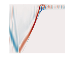
  $N = 1 \times 10^{-3}\,\textrm {s}^{-1}$. An example of the initial state is plotted in figure 1.

Figure 1. An example of the initial velocity fields (shaded) overlaid with density contours. (a) The initial along-shelf velocity  $v(x,z,0) = V(x)$ with
  $V_{max} = 1\,\textrm {m}\,\textrm {s}^{-1}$,
  $x_0 = 50$ km and
  $x_r = 60$ km. The barotropic tidal current is initially zero. (b) The initial cross-shelf current
  $u$, which is equal to the maximum on-shelf barotropic current. Here
  $A = 0.02$ in the deep water.
The parameters that can be varied under this setting are:
 \begin{equation} \left. \begin{aligned} f: & \quad the\ Coriolis\ parameter; \\ s: & \quad the\ slope\ of\ the\ bathymetry;\\ x_0: & \quad the\ location\ of\ the\ center\ of\ the\ current;\\ V_{max}: & \quad the\ velocity\ of\ the\ geostrophic\ current\ at\ x=x_0;\\ x_r: & \quad the\ width\ of\ the\ current. \end{aligned} \right\} \end{equation}
We consider bathymetries with slope  $s$ so that in the absence of a current, the slope criticality
  $\alpha = s/\gamma \approx$ 0.8. Our setting of the geostrophic current implies the Rossby number
  $Ro = O(V_x/f) = O(0.1)$. The values of the relevant parameters are listed in table 1. We choose these parameters to represent real world ocean currents. For example, the current width is modelled by
  $4x_r$. In the Northern Hemisphere, negative
  $V_{max}$ can represent western boundary currents flowing north or eastern boundary currents flowing south. Western boundary currents are generally faster and narrower than eastern boundary currents. The Gulf Stream has an average speed of
  $1.8\,\textrm {m}\,\textrm {s}^{-1}$ and a typical width of 100 km. The mean speed of the southward flowing California current is
  $0.1\,\textrm {m}\,\textrm {s}^{-1}$ and its width is between 500 and 800 km. However, positive
  $V_{max}$ can represent western boundary currents flowing south or eastern boundary currents flowing north. The southward flowing Labrador Current has a typical speed of approximately 0.4
  $\textrm {m}\,\textrm {s}^{-1}$ and it is approximately 100 km wide. Speeds of the northward flowing Norwegian Coastal Current can vary greatly from 0.1
  $\textrm {m}\,\textrm {s}^{-1}$ to 1
  $\textrm {m}\,\textrm {s}^{-1}$ depending on the season. These large ranges of
  $V_{max}$ and
  $x_r$ are covered in our choice of parameters. We vary the current centre
  $x_0$ to model the different locations of the current relative to the bathymetry. In particular, because the focus of this paper is on near-critical latitudes, a larger parameter space was done with
  $f = 6.7 \times 10^{-5}\,\textrm {s}^{-1}$ (
 $\approx$27.5
  $^{\circ }$N) than that with
  $f = 6.0 \times 10^{-5}\,\textrm {s}^{-1}$ (
 $\approx$24.5
  $^{\circ }$N).
Table 1. Parameter space.

The central domain of interest has a length  $L=$ 200 km with uniform resolution
  ${\textrm {d}\kern0.06em x} = 25$ m. The vertical grid is non-uniform with a total of
  $nz =$ 400 points, in which 80 points are in the shallow water. The finest resolution is
  $\textrm {d}z =$ 2.5 m in the upper 200 m and it linearly stretches to
  $\textrm {d}z =8$ m in the deep water. On either side of the central domain, there is a layer in which the grid is slowly stretched horizontally with successive grid cell lengths increased by
  $0.5\,\%$. Each simulation is run for 60 tidal periods. The total domain is long enough so that no ITs can reach the boundaries within the simulation time. The model time step is 6 s.
The horizontal viscosity is parametrized with a nonlinear Smagorinsky scheme (Smagorinsky Reference Smagorinsky1993) with viscC2Smag = 2. We use PP81 to model the vertical viscosity  $\mu$ and diffusivity
  $\kappa$ (Pacanowski & Philander Reference Pacanowski and Philander1981; Stashchuk et al. Reference Stashchuk, Vlasenko, Hosegood and Nimmo-Smith2017).
3. Calculation of conversion rate
To calculate the barotropic to baroclinic conversion rate, the velocity, density and pressure fields are first separated into barotropic and baroclinic fields following Kang & Fringer (Reference Kang and Fringer2012). The total flow field is divided into
 $$\begin{gather} {\boldsymbol u} = (u, v, w) = (U_{bt}+u', V_{bt}+V+v', W_{bt}+w'), \end{gather}$$
 $$\begin{gather}\rho = \rho_b(z) + \rho'(x,z,t), \end{gather}$$
 $$\begin{gather}p = p_b(z) + p_g(x) + p_{bt}(x,z,t) + p'(x,z,t), \end{gather}$$
where  ${\boldsymbol U_{bt}} = (U_{bt}, V_{bt}, W_{bt})$ is the velocity field associated with the barotropic tidal currents and
  ${\boldsymbol u'} = (u',v',w')$ is the perturbation velocity. Using an overbar above a quantity
  $\phi$ refers to the depth integral
  $\bar {\phi } = \int _{-h}^{0} \phi \, dz$, the barotropic current is defined as
 $$\begin{gather} U_{bt}(x,t) = \frac{1}{h(x)} \bar{u}, \end{gather}$$
 $$\begin{gather}V_{bt}(x,t) = \frac{1}{h(x)} \bar{v}, \end{gather}$$
 $$\begin{gather}W_{bt}(x,z,t) ={-} \frac{\partial U_{bt}}{\partial x} z. \end{gather}$$
Here,  $\rho _b(z)$ is the background density field in hydrostatic balance with
  $p_b(z)$. We take
  $p_b = 0$ at the surface. The
  $p_g(x)$, given by
  $\partial p_g/\partial x = f\kern0.06em V$, is the pressure associated with the geostrophic current
  $V$. We take
  $p_g=0$ to the left of the current. Here,
  $\rho '(x,z,t)$ is the density perturbation in hydrostatic balance with
  $p_{bt} + p'$, where
  $p_{bt}$ and
  $p'$ are the barotropic and baroclinic pressure, respectively. We assume
  $p'$ has zero depth average (Kunze et al. Reference Kunze, Rosenfeld, Carter and Gregg2002), i.e.
  $p' = (p-p_b) - {1}/{h(x)} \overline {(p-p_b)}$, and
  $\rho '$ is assumed to be the baroclinic density perturbation.
The total barotropic-to-baroclinic energy conversion is given by  $C = \iint \rho ' g W \,{\textrm {d}\kern0.06em x}\, \textrm {d}z$. In particular,
  $C$ is the horizontal integration of the conversion
  $\bar {C} = \int \rho ' g W \,\textrm {d}z$. Here,
  $\bar {C}(x,t)$ can be either positive or negative. Positive conversion means energy is converted from barotropic to baroclinic tides, while negative conversion means energy is transferred from baroclinic to barotropic tides. We denote
  $C_p(t) = \varSigma _{\bar {C}>0} \bar {C}\,{\textrm {d}\kern0.06em x}$ and
  $C_n(t) = \varSigma _{\bar {C}<0} \bar {C} \,{\textrm {d}\kern0.06em x}$. The summation is over all grid columns and multiplied by the horizontal spacing
  ${\textrm {d}\kern0.06em x}$. All the values of the conversion rate are averaged over one tidal period.
4. Simulation results
Owing to the large number of simulations done, only selected cases are presented here. Two series of simulations, A and B, were undertaken. They are for Coriolis frequencies  $f = 6.7 \times 10^{-5}\,\textrm {s}^{-1}$ and
  $6.0 \times 10^{-5}\,\textrm {s}^{-1}$, respectively. Table 2 lists the parameters used for the two series. We define
  $r_m$ as the part of the slope where
  $\alpha > 0.99 \alpha _{max}$ and
  $r_b$ as the
  $x$ value of the location around which the beam is emitted. Here,
  $\alpha _{max}$ is the maximum value of the criticality parameter
  $\alpha$, and
  $x_c$ and
  $x_{c0}$ are critical points. The slope is supercritical (subcritical) to the left (right) of
  $x_c$, and vice versa for
  $x_{c0}$. A stretch of the slope with
  $f_{eff} > \sigma _T$ is called a blocking region. The slope criticality
  $\alpha$ is undefined in blocking regions. The details on
  $f_{eff}$,
  $\gamma$,
  $C$ and
  $C_{p(n)}$ for each case are plotted in figure 2.
Table 2. Parameters in A and B series. Here,  $V_{max}$,
  $x_0$ and
  $x_r$ are maximum velocity, the centre and the width of the current. Additionally,
  $r_m$ is the part of the slope where
  $\alpha > 0.99 \alpha _{max}$,
  $x_c$ and
  $x_{c0}$ are critical points, and
  $r_b$ is the
  $x$ value of the location around which the beam is emitted.


Figure 2. (a,c,e,g) A series (magenta, black, black dashed, black dotted, black dash–dotted, blue) = (A0, A1, A2, A3, A4, A5). (b,d,f,h) B series (magenta solid, black, black dashed, blue, blue dashed) = (B0, B1, B2, B3, B4). (a,b) Effective frequencies. Magenta dashed (solid) line is  $\sigma _T$ (
 $f$). (c,d) Slope of IT characteristics
  $\gamma$. The red line is the bathymetric slope. (e,f) Total conversion rates
  $C$. (g,h)
  $C_p$ and
  $C_n$.
4.1. Scenario I: no current
We begin with the simplest cases A0 and B0 for which there are no background currents (magenta solid lines in figure 2). These provide a reference for cases with currents. The shelf slope lies between 0 and 81 (55) km for the A (B) series. We can see a large transient behaviour in the time evolution of the conversion rate  $\bar {C}$ (figures 2e,f and 3a,b). At the beginning of the simulations, the wave field needs time to adjust to the sudden onset of the tidal forcing. It takes approximately 10 and 5 tidal periods for A0 and B0 to reach a quasi-steady state. Here
  $\alpha$ is constant on the majority of the slope and ITs are generated along the whole slope. The bathymetry is smoothed out near the bottom, so
  $\alpha$ is small near the base at
  $x=0$ and near the shelf break, and it has its maximum value at the centre of the slope. For these cases,
  $r_m$ is approximately the region (5 km, shelf break
  $-$ 5 km). For both cases, IT beams are emitted from a neighbourhood of
  $r_b \approx 20$ km (figure 3g,h) approximately 100 m above the bottom (figure 3c,d). To the left of
  $r_b \approx$ 20 km is a beam with
  $\boldsymbol {c}_g$ propagating to the base of the slope then reflecting up to the left, and to the right a more intense beam propagates to the upper right. The phase of the rightward beam propagates downward (figure 3e,f) and the energy goes upward until it hits the surface and gets reflected (figure 3g,h). The characteristic IT beam path shown in green (figure 3c,d) is in general calculated using a ray-tracing technique although in the absence of a background current, they are straight lines. The beam energy continues to propagate onshore while being reflected by the surface and bottom. The beams generated near
  $r_m$ are a common feature in all of our simulations, and it is related to positive conversion
  $C_p$. Each time the beam reflects, the sign of the conversion
  $\bar {C}$ changes (figure 3a,b).

Figure 3. (a,c,e,g) Case A0. (b,d,f,h) Case B0. (a,b) Contour plot of the vertical integration of  $\bar {C}$ (
 $\textrm {W}\,\textrm {m}^{-2}$) varying on the spatial and time scales. (c,d) Contour of the density perturbation
  $\rho '$ at the end of 30 tidal periods. Green lines are the characteristics of IT beams. Green circles mark the location where the beam is emitted. (e,f) The horizontal baroclinic velocity
  $u'$: (e)
  $x = 40$ km; (f)
  $x = 30$ km. (g,h) Energy flux
  $\langle (u',w')p'\rangle$.
4.2. Scenario II: no critical point
We include a current  $V(x)$ with relatively small
  $V_x$ so that
  $\alpha <1$ everywhere. We consider cases B2 and B4, which only differ in the sign of
  $V_{max}$ (blue dashed and black dashed lines in figure 2b,d,f,h). Unlike the cases A0 and B0, the slope criticality
  $\alpha$ here varies along the slope owing to the presence of the current. In B2 (positive current),
  $\alpha$ is increased (decreased) to the left (right) of the current centre
  $x_0$, with
  $\alpha$ reaching its maximum near the bottom at
  $r_m \approx 10$ km and its minimum is at
  $x \approx 50$ km. Two beams emanate from
  $r_b \approx 25$ km (figure 4c,g). This difference in the
  $x$-location between beam emission and
  $\alpha _{max}$ (
 $r_b$ and
  $r_m$) is presumably owing to the strengthening of the barotropic current with decreasing water depth. To the right of
  $r_b \approx 25$ km, the phase of the beam propagating downwards (figure 4f) indicates that energy propagates upwards (figure 4h). Note the slope of the beam is curved owing to the varying
  $f_{eff}$. The beam is emitted from a location similar to that in case B0 but the slope is closer to critical with
  $\alpha _{max} = 0.97$. As a result, the total conversion rate
  $C$ in B2 is larger than in case B0 (black dashed line in figure 2f).

Figure 4. Same as figure 3, except for case B2, with  $V_{max} =$ 0.5
  $\textrm {m}\,\textrm {s}^{-1}$ (a,c,e,g) and case B4, with
  $V_{max} = -0.5\,\textrm {m}\,\textrm {s}^{-1}$ (b,d,f,h). The cyan diamond marks
  $r_m$ where
  $\alpha _{max}$ occurs. Green circles mark the location where the beam is emitted. Again, (e)
  $x = 40$ km, (f)
  $x = 30$ km.
In B4 with  $V_{max} = -0.5\,\textrm {m}\,\textrm {s}^{-1}$,
  $\alpha _{max} =$ 0.97 occurs near the shelf break (
 $r_m \approx 45$ km) and it is smallest at
  $x \approx 15$ km. Three beams are emitted from the left and right of
  $r_b \approx r_m$ (figure 4d) Because the slope is subcritical on both sides of
  $r_b$, for the left downward propagating beam to be generated, the generation location must be above the slope. To verify this beam pattern, an extra simulation was conducted in which the water depth was increased by 400 m everywhere and the deep water barotropic current was increased so that the same barotropic tidal forcing is applied in the shallow water region. This makes the three IT beams more distinguishable. Details are omitted here. To the upper-left of
  $r_b$ there is a wide beam, and to the lower-left and right of
  $r_b$ there are two narrow beams. They each propagate onwards until hitting the surface/bottom, as illustrated in figure 4(d,h) for case B4. The upward phase propagation at
  $x = 30$ km (figure 4f) confirms the downward
  $\boldsymbol {c}_g$ propagation. Owing to the different beam patterns in B4, the region of positive
  $C_p$ (negative
  $C_n$) conversion (figure 4b) is different from those in cases B2 and B0. Here,
  $C_p$ in B4 only exists for
  $x> 30$ km, which results a smaller total conversion rate
  $C$ (dashed lines in figure 2f,h).
4.3. Scenario III: No blocking + critical point
We now double the current so that  $\alpha \ge$ 1 for some portion of the slope. We consider cases B1 with
  $V_{max} = 1\,\textrm {m}\,\textrm {s}^{-1}$ and B3 with
  $V_{max} = -1\,\textrm {m}\,\textrm {s}^{-1}$ (black and blue lines in figure 2b,d,f,h). There are two critical points in both cases.
In B1, one critical point  $x_c =$ 30 km lies in the middle of the slope and the other
  $x_{c0} =$ 3 km is near the bottom. Between these two critical points, the slope is supercritical. There are two intense beams emanating from
  $r_b \approx$ 35 km near
  $x_c$ (figure 5g) but no beams near
  $x_{c0}$. This is because the slope is supercritical (subcritical) to the left (right) of
  $x_c$. However, the slope is subcritical (supercritical) to the left (right) of
  $x_{c0}$. No beams with a positive slope can be emitted from
  $x_{c0}$. Note the beam generation location
  $r_b$ is up-slope of
  $x_c$ owing to the strengthening of the barotropic current in the shallower water. An intense beam is emitted from the right of
  $r_b$ and propagates upwards until it hits the surface at approximately
  $x = 53$ km (figure 5c). It gets reflected from the surface and keeps propagating onto the shelf while being reflected between the surface and the bottom. Analogously, the other intense beam emanates from the left of
  $r_b$ with phase propagating upwards (figure 5e) and energy propagating downward (figure 5g) until it hits the bottom at approximately
  $x = -10$ km and gets reflected. The reflection location corresponds to the change of sign of
  $\bar {C}$ (figure 5a). The conversion rate
  $\bar {C}$ vanishes around
  $x = -10$ km because the bathymetry is flat and
  $W = 0$.

Figure 5. Same as figure 3, except for case B1 (a,c,e,g) and case B3 (b,d,f,h). The cyan diamonds mark the critical points  $x_c$ and
  $x_{c0}$. Green circles mark the location where the beam is emitted. Here, (e)
  $x =20$ km, (f)
  $x = 30$ km.
In case B3, the two critical points are at  $x_c = 53$ km near the shelf break and
  $x_{c0} = 31$ km in the middle of the slope. The slope is subcritical (supercritical) to the left (right) of
  $x_{c0}$, while it is the other way around for
  $x_c$. As a result, beams can be generated at
  $r_b = x_c$ but not at
  $x_{c0}$. Three beams are emitted from
  $r_b = 53$ km (figure 5d). One beam emanates from the right of
  $r_b$ and propagates to the upper right. Two beams emanate from the left of
  $r_b$. One of them propagates downwards until it reflects from the bathymetry at
  $x = 13$ km. The other beam propagates upwards and reflects from the surface at
  $x = 40$ km, where the reflected beam subsequently propagates downward until it hits the bottom at
  $x = -5$ km. The upward phase propagation at
  $x = 30$ km (figure 5f) confirms the downward energy propagation. Similar to case B4, a separate simulation with water depth increased by 400 m everywhere has been conducted to verify this beam pattern. Details are omitted here. The three beams emitted directly from
  $r_b$ contribute to the positive conversion
  $C_p$, while their reflected beams contribute to the negative conversion
  $C_n$. The resulting conversion rate pattern
  $\bar {C}$ (figure 5b) is a combination of
  $C_p$ and
  $C_n$.
Because strong generation occurs near the critical point  $x_c$, B1 and B3 have the largest total conversion rate
  $C$ in the B series (black and blue in figure 2f). However, owing to the different beam patterns, B3 has a much larger region of negative
  $C_n$ than B1 (figure 5a,b). As a result, B3 has a smaller
  $C$ than B1 (black and blue lines in figure 2f,h).
4.4. Scenario IV: blocking near the bottom/shelf break
We now consider a strong current such that  $f_{eff} > \sigma _T$ along a stretch of the slope which we call a blocking region. Freely propagating internal waves do not exist in this region but tunnelling may occur. We analyse results from the A series with a focus on cases A1 (
 $V_{max} = 1$
  $\textrm {m}\,\textrm {s}^{-1}$) and A5 (
 $V_{max} = -1\,\textrm {m}\,\textrm {s}^{-1}$). For this series, the slope lies between
  $x = 0$ and 81 km.
In A1, there is a blocking region,  $x \in [-5, 26]$ km, near the bottom of the slope (black line in figure 2c). There is a critical point at
  $x_c = 45$ km. To the left (right) of the critical point, the slope is supercritical (subcritical). Two strong narrow IT beams are emitted from
  $r_b \approx 55$ km near
  $x_c$ (figure 6c,g). This pattern is similar to case B1. The difference is, here, the amplitude of the beams with tidal frequency
  $\sigma _T$ decays quasi-exponentially to the left in the region
  $-5$ km
  $\le x \le$ 26 km, where
  $f_{eff} > \sigma _T$. IT beams cannot be generated in this blocking region either. As a result, the conversion
  $C$ in the blocking region is very weak (figure 6a). For
  $x > 26$ km, the change of sign in
  $C$ follows the IT beam reflection location.

Figure 6. Same as figure 3, except for case A1 (a,c,e,g) and case A5 (b,d,f,h). The cyan diamonds mark the critical points  $x_c$ and
  $x_{c0}$. Green circles mark the location where the beam is emitted. The red lines mark the edges of the blocking region. Here, (e)
  $x= 60$ km, (f)
  $x= 40$ km.
Relative to A1, the centre of the current  $x_0$ in cases A2, A3 and A4 is shifted up or down slope (figure 2a). There is a critical point
  $x_c$ and a blocking region in each of these four cases. In general, the conversion rate
  $C$ increases as
  $x_c$ moves closer to the shelf break, because the barotropic tidal forcing reaches its maximum in the shallow water. In this case, we have
  $C(A3) > C(A1) > C(A2)$ (figure 2c). However, as the blocking region gets closer to the shelf break,
  $C$ decreases explaining
  $C(A3) > C(A4)$.
In case A5, the current is negative and the blocking region,  $x \in [65, 100]$ km, is near the shelf break (blue line in figure 2c). There is a critical point
  $x_{c0} = 50$ km, but no beams with positive slope can be emitted there because the slope is subcritical (supercritical) to the left (right) of
  $x_{c0}$. Because beams with tidal frequency cannot propagate upward owing to the blocking region and the slope is supercritical to the right of
  $x_{c0}$, two leftward propagating beams are generated approximately 300 m above the slope at
  $r_b \approx 65$ km, which is near the edge of the blocking region (figure 6d,h). One beam propagates downward and hits the slope at
  $x = 10$ km. The other beam propagates upwards and gets reflected at the surface
  $x = 50$ km. The upward phase propagation at
  $x = 40$ km (figure 6f) confirms the downward energy propagation. A separate simulation with water depth increased by 400 m everywhere has been conducted to confirm this beam pattern. Details are omitted here. The reflected (pre-reflected) beam contributes to the negative (positive) conversion
  $C_n$ (
 $C_p$). The resulting conversion pattern is a combination of these two (figure 6b). This puts
  $C(A5)$ as the smallest among the five cases with currents in the A series.
5. Discussion and summary
How the current parameters influence the total conversion  $C$ is a complex problem. We illustrate it by conducting extra simulations and plotting the relation between
  $C$ and the location of the current centre
  $x_0$ for different current widths (figure 7). When
  $V_{max}$ is positive,
  $f_{eff} > f$ to the left of
  $x_0$ (deeper water) and
  $f_{eff} < f$ to the right of
  $x_0$ (shallower water) in the Northern Hemisphere where
  $f>0$, which we have assumed throughout. As a consequence, IT characteristic slopes
  $\gamma$ are reduced and the slope criticality
  $\alpha$ is increased to the left of
  $x_0$ while the opposite happens to the right of
  $x_0$. Here,
  $C$ peaks when
  $x_0$ is placed in a position such that the portion of the slope that is near critical is maximized. In particular, the upper slope including the shelf break plays a dominant role because the tidal forcing there is the strongest. We can see this pattern in figure 7(a) with a small exception in the case of the narrowest current (black solid line): there are two local peaks when
  $(V_{max}, x_r) = (1\,\textrm {m}\,\textrm {s}^{-1},\ 60\,\textrm {km})$. A blocking region exists to the left of
  $x_0$ for this case but not in the cases with wider currents because the velocity gradients are reduced as
  $x_r$ increases. Note cases A1 to A4 are included in this line and we can refer to figure 2(c) for
  $f_{eff}$ for these cases. When
  $x_0$ increases from 25 km near the bottom of the slope,
  $C$ increases because the critical point
  $x_c$ is shifted closer to the shelf break with stronger tidal forcing. However as
  $x_0$ increases further,
  $C$ decreases because the blocking region is moving to the shelf break where most of the generation occurs. This creates a first local peak at
  $x_0 = 75$ km with the blocking region extending between 22 and 54 km. Subsequently,
  $C$ increases again as the blocking region moves onto the shelf creating a second local peak at
  $x_0 = 123$ km. This second peak has a much larger
  $C$ than the first peak because the slope criticality
  $\alpha$ is larger to the left of
  $x_0$. With
  $x_0$ on the shelf, only the left part of the current affects the value of
  $\alpha$. If we increase the current width
  $x_r$, there is no blocking region and the maximum
  $C$ occurs at a location with
  $x_0$ on the shelf. Cases with
  $x_r = 105$ km (blue solid line) produce the largest
  $C$ among the four lines. This is because the conversion rate
  $C$ is determined by the two aspects of the slope criticality
  $\alpha$, its magnitude and the portion of the slope where
  $\alpha$ is large. With a wider current,
  $\alpha$ is reduced but the region of the shelf slope with increased slope criticality increases.

Figure 7. (a) Positive currents with  $V_{max} = 1\,\textrm {m}\,\textrm {s}^{-1}$. Current width
  $x_r$ in (black solid, black dashed, blue solid, blue dashed) = (60 km, 75 km, 105 km, 160 km). (b) Negative currents. Here,
  $V_{max}$ in (black solid, black dashed, blue) = (
 $-1\,\textrm {m}\,\textrm {s}^{-1}$,
  $-1\,\textrm {m}\,\textrm {s}^{-1}$,
  $-0.5\,\textrm {m}\,\textrm {s}^{-1}$).
  $x_r$ in (black solid, black dashed, blue) = (60 km, 75 km, 60 km). For both panels (a,b),
  $f = 6.7 \times 10^{-5}\,\textrm {s}^{-1}$. Shelf break is at 80 km. Magenta line is
  $C$ without a current (case a0). Empty circles represent the numerical simulations.
Results for negative currents are shown in figure 7(b). As  $V_{max}$ changes sign, the behaviour of
  $f_{eff}$ and
  $\alpha$ reverses too. The slope is closer to being critical to the right of
  $x_0$, meaning the peak of
  $C$ occurs when the centre of the current is in deeper water (smaller
  $x_0$) than in the case of positive currents. Currents in the black solid line are stronger (
 $V_{max} = -1\,\textrm {m}\,\textrm {s}^{-1}$) than those in the blue solid line (
 $V_{max} = -0.5\,\textrm {m}\,\textrm {s}^{-1}$). However, the stronger currents have a generally smaller
  $C$ owing to the presence of a blocking region (located to the right of
  $x_0$). Apart from these general statements, the exact magnitude of
  $C$ is also affected by the contribution of
  $C_p$ and
  $C_n$, which is predicted by the beam pattern. As a result, there is a sharp decrease in
  $C$ as
  $x_0$ approaches 40 km.
The positive currents can increase the conversion rate  $C$ by up to 10 times (blue solid line in figure 7a) compared with case A0 (no current). The negative currents can also increase
  $C$ but generally not so much as the positive currents do. This asymmetry can be seen using an example of how
  $C$ varies with different
  $V_{max}$ plotted in figure 8. The current width
  $x_r$ and centre
  $x_0$ are the same as those of case A1. By reversing the sign of
  $V_{max}$, the variation of
  $f_{eff}$ to the left and right of
  $x_0$ is reversed leading to different beam patterns. The two local peaks near
  $V_{max} = 0.6\,\textrm {m}\,\textrm {s}^{-1}$ and
  $-1\,\textrm {m}\,\textrm {s}^{-1}$ are a result of a blocking region from increasing
  $|V_{max}|$. As
  $|V_{max}|$ increases from 0,
  $C$ first increases as a result of the rising slope criticality
  $\alpha$. Then
  $C$ decreases owing to the increasing size of the blocking region.

Figure 8. Conversion rate  $C$ as a function of
  $V_{max}$. Here,
  $f = 6.7 \times 10^{-5}\,\textrm {s}^{-1}$,
  $(x_0, x_r) =$ (50 km, 60 km).
We summarize how the presence of a geostrophic barotropic current  $V(x)$ affects the conversion rate.
(i) The
 $V(x)$ changes the effective frequency from $f_{eff}^{2} = f^{2}$ to $f_{eff}^{2} = f^{2} + f\kern0.06em V_x$. This has a direct impact on the slope of the IT characteristics $\gamma$ and the slope criticality $\alpha = s/\gamma$. It has been shown previously that $\alpha$ is a crucial factor in determining the total conversion $C$ (e.g. Bell Reference Bell1975; Baines Reference Baines1982; Balmforth et al. Reference Balmforth, Ierley and Young2002).
(ii) Because
$V_x$ is not a constant value, $f_{eff}$ varies along the slope. This has a significant effect on IT beam generation location $r_b$ and their propagation paths. When $f_{eff} < \sigma _T$, internal waves are generated everywhere along the slope. The intensity of the IT beams depends on the current, which also determines the beam generation location $r_b$. Here, $r_m$ is defined as the part of the slope where $\alpha > 0.99 \alpha _{max}$ and $r_b$ is usually equivalent to or slightly larger than the upper bound of $r_m$ because tidal forcing increases as the water depth decreases. With a slightly stronger current such that part of the slope is critical/supercritical, IT beams can be emitted near a critical point $x_c$ if the slope is of the same sign as the slope of the beam and it is subcritical (supercritical) to the left (right) of $x_c$ but not the other way around. With a strong current such that part of the slope acts as a blocking region where $f_{eff} > \sigma _T$, IT beams are emitted near a critical point and the conversion rate $C$ becomes extremely small in the blocking region.(iii) The change of sign in
$\bar {C}$ corresponds to the IT beam reflection location. As a result, the total conversion rate $C = C_p + C_n$ is also strongly affected by the IT beam pattern, which depends on $V_x$.


In conclusion, the total conversion rate  $C$ is affected by a combination of three factors: slope criticality
  $\alpha$, the size and location of the blocking region where ITs cannot be generated, and the IT beam pattern including where the beams are emitted and reflected, all of which can be varied by the geostrophic current
  $V$. In this paper, we assumed
  $f > 0$, i.e. the Northern Hemisphere, and
  $K_1$ diurnal tides as the forcing. Our work can be extended to the Southern Hemisphere by simply reversing the signs of
  $f$ and
  $V_{max}$. It can also be applied to any other tidal constituents as long as
  $f$ is close to the tidal frequency so that
  $\sigma _T^{2} - f_{eff}^{2} = \sigma _T^{2}-f^{2}-f\kern0.06em V_x$ in (1.1) can vary significantly by varying
  $V_x$. This is easiest if
  $\sigma _T^{2}-f^{2}$ is small. What matters is the dimensionless parameter
  $\tilde {f} = f/\sigma _T$. In our paper,
  $\tilde {f} \ge$ 0.82. At latitudes far from critical, i.e.
  $f \ll \sigma _T$ and
  $\tilde {f} \ll 1$, the slope criticality will be modified by
  $V_x$ but the effects are expected to be reduced. As a result, the conversion rate is modified but not as much as that of the near-critical latitudes.
Although we considered idealized cases that use a linear stratification and a symmetric barotropic current, the key point of this work is that the current changes  $f_{eff}$ which changes the conversion. This is unlikely to change in a more realistic setting. For example, with a varying
  $N(z)$ in the absence of a current, the IT beams will bend instead of following a straight line. However, the presence of a current would affect how the beam bends and the slope criticality in the same way that we have described in this paper. Including baroclinic currents is an important future problem of this research, because it introduces horizontal density gradients. Other important future avenues of this research are to incorporate asymmetric currents and more realistic bathymetry. The effects of background currents on PSI, which can occur at lower latitudes where
  $2 f_{eff} \approx \sigma _T$ is the subject of ongoing work.
Funding
This work is supported by grants from the Natural Sciences and Engineering Research Council of Canada and from the Canadian Foundation for Innovation and the Ontario Research Fund. The facilities of the Shared Hierarchical Academic Research Computing Network (SHARCNET: https://www.sharcnet.ca) and Compute/Calcul Canada were used for this work.
Declaration of interests
The authors report no conflict of interest.


