2.1. Derivation of a Cox type model for the apparent contact angle

It is known that the two-phase flow has a multiscale property near moving contact lines. In general, the macroscopic contact angle is different from the microscopic one; see for example Cox (Reference Cox1986), where a dynamic boundary condition for the apparent contact angle was derived by matched asymptotic analysis. In the following, we derive a similar boundary condition by using the Onsager principle as an approximation tool. The derivation is much simpler but still captures the essential dynamics of the apparent contact angle. In Appendix A, we show that the variational principle can also be used to derive a full continuum model for moving contact lines.

As shown in figure 1, we separate the domain near the contact line into three different scales. The macroscopic region $\varOmega$ has a characteristic length $L$. The microscopic region is of molecular scale with a characteristic length $l$. In the microscopic scale, the interaction between the liquid molecules and the solid molecules induces a friction of the contact line (Guo et al. Reference Guo, Gao, Xiong, Wang, Wang, Sheng and Tong2013). The mesoscopic region has a characteristic length $D\ll L$, but still much larger than the molecular scale $l$. In this region, the no-slip boundary condition is still a good approximation. The contact angle $\theta _a$ represents the apparent angle in macroscopic point of view.

Figure 1. The region near the moving contact point in different scalings($l\ll D\ll L$).

We are interested in the contact line dynamics in the mesoscopic region. For this purpose, we analyse the system by using the Onsager principle as an approximation tool. We make the ansatz that the interface between the two fluids in this region can be approximated well by a straight line $\tilde {\varGamma }$ which has a tilting angle equal to the macroscopic contact angle $\theta _a$. With this assumption, we can use the Onsager principle to derive a relation between the apparent contact angle $\theta _a$ and the contact line motion as follows.

We first calculate the rate of change in the total free energy of the system. Similar to (A1), the total approximate free energy $\tilde {\mathcal {E}}$ is composed of three surface energies. The changing rate of the total interface energies with respect to the motion of the contact line is given by

(2.1)\begin{equation} \dot{\tilde{\mathcal{E}}}=\gamma(\cos\theta_a-\cos\theta_Y)v_{ct} + \int_{\tilde{\varGamma}} \gamma\kappa v_n \,{\rm d}s= \gamma(\cos\theta_a-\cos\theta_Y)v_{ct}. \end{equation}

Here γ is the fluid–fluid surface tension, $v_{ct}$ is the contact line velocity, $\theta_Y$ is the Young's angle, $\kappa$ and $v_n$ are respectively the curvature and the normal velocity of the fluid–fluid interface; the second term disappears since the curvature is zero for a straight line. To use the Onsager principle for the open system, we need consider the work to the exterior region on the outer boundary, $\dot {\tilde {\mathcal {E}}}^{*}=-\int _{\tilde {\varGamma }_{out}} \boldsymbol {F}_{ext}\boldsymbol {\cdot } \boldsymbol {v}$, with $\boldsymbol {F}_{ext}$ being the external force. This is a higher-order term in comparison with $\dot {\tilde {\mathcal {E}}}$, since it is of order $|\boldsymbol {F}_{ext}| v_{ct} D$ with $D\ll L=O(1)$. We will ignore this term in the following calculations.

We now compute the energy dissipations in the wedge region as shown in figure 1 (right plot). The total energy dissipation is calculated approximately as

(2.2)\begin{equation} \tilde{\varPsi}={\xi}v_{ct}^{2}+\int_{\tilde\varOmega_A}{\dfrac{\mu_A}{4} |\boldsymbol{\nabla} \boldsymbol{v}+\boldsymbol{\nabla} \boldsymbol{v}^{\rm T}|^{2}} \,{{\rm d}\kern0.06em x}+\int_{\tilde\varOmega_B}{\dfrac{\mu_B}{4} |\boldsymbol{\nabla} \boldsymbol{v}+\boldsymbol{\nabla} \boldsymbol{v}^{\rm T}|^{2}} \,{{\rm d}\kern0.06em x}, \end{equation}

In the above formula, $\tilde {\varOmega }_A$ and $\tilde {\varOmega }_B$ are the domains corresponding to liquids $A$ and $B$ in the mesoscopic region, $\mu_A$ and $\mu_B$ are respectively the viscosities of fluids A and B, and the superscript T stands for the transpose of a matrix. The contact line friction term ${\xi }v_{ct}^{2}$ is due to the dissipation in the microscopic region and $\xi$ is the friction coefficient. The velocity $\boldsymbol {v}$ can be obtained by solving the Stokes equations in wedge regions assuming the interface moving in a steady state. By careful calculations (see Appendix A), we can compute the energy dissipation function approximately

(2.3)\begin{equation} \tilde{\varPhi}=\dfrac{1}{2}\tilde{\varPsi}\approx \dfrac{1}{2}{\xi}v_{ct}^{2}+\dfrac{\mu_A |\ln\zeta|}{2\mathcal{F}(\theta_a,\lambda)}v_{ct}^{2}, \end{equation}

where the dimensionless parameter $\zeta =D/l$ is the ratio between the mesoscopic size and the microscopic size, and

(2.4)\begin{align} &\mathcal{F}(\theta_a,\lambda)\nonumber\\ &\quad =\dfrac{\lambda(\theta_a^{2}-\sin^{2}\theta_a)({\rm \pi}-\theta_a+\sin\theta_a\cos\theta_a)+(({\rm \pi}-\theta_a)^{2}-\sin^{2}\theta_a)(\theta_a-\sin\theta_a\cos\theta_a)}{2\sin^{2}\theta_a\left(\lambda^{2}(\theta_a^{2}-\sin^{2}\theta_a) +2\lambda(\sin^{2}\theta_a+\theta_a({\rm \pi}-\theta_a))+(({\rm \pi}-\theta_a)^{2}-\sin^{2}\theta_a)\right) }, \end{align}

with $\lambda ={\mu _B}/{\mu _A}$. The contact line friction can be understood from the molecular kinetics theory (Blake & Haynes Reference Blake and Haynes1969; Blake Reference Blake2006; Blake & De Coninck Reference Blake and De Coninck2011). Molecular dynamic simulations have been done in Johansson & Hess (Reference Johansson and Hess2018) to compute the friction coefficient. For a water–air interface on a clean glass substrate, the coefficient $\xi$ is measured directly in experiments in Guo et al. (Reference Guo, Gao, Xiong, Wang, Wang, Sheng and Tong2013), which is given by $\xi \approx (0.8\pm 0.2)\mu$. Notice that $\ln \zeta$ is generally chosen as a constant of order $10$ (in de Gennes, Brochard-Wyart & Quere (Reference de Gennes, Brochard-Wyart and Quere2003), it is chosen as $13.6$). Direct computations also show that $1/\mathcal {F}(\theta _a,\lambda )=O(1)$. In this case, $\xi$ can be regarded a small perturbation to the viscous friction coefficient and can be ignored. More detailed discussions on the contact line friction can be found in Duvivier, Blake & De Coninck (Reference Duvivier, Blake and De Coninck2013). It is found that the friction coefficient $\xi$ is proportional to the viscosity of the liquid and exponentially dependent on the strength of solid–liquid interactions. The value of $\xi$ can range over several magnitudes for various systems.

By using the Onsager principle, we minimize the Rayleighian $\mathcal {R}=\tilde {\varPhi }+ \dot {\tilde {\mathcal {E}}}$ with respect to $v_{ct}$. This leads to an equation for $v_{ct}$

(2.5)\begin{equation} {\left(\xi+\dfrac{\mu_A |\ln\zeta|}{\mathcal{F}(\theta_a,\lambda)}\right)}v_{ct}={-}\gamma(\cos\theta_a-\cos\theta_Y). \end{equation}

This equation basically means that the local dissipative force (due to the contact line friction and the viscous dissipation) is balanced by the effective unbalanced Young's force, which is the dominant term in the driving force in the mesoscopic region. It gives a relation between the contact line velocity and the apparent contact angle $\theta _a$. The relation (2.5) can be rewritten in a dimensionless form

(2.6)\begin{equation} \left(\alpha + \dfrac{|\ln\zeta|}{\mathcal{F}(\theta_a,\lambda)}\right)Ca={-}(\cos\theta_a-\cos\theta_Y), \end{equation}

where $\alpha ={\xi }/{\mu _A}$ and $Ca={\mu _A v_{ct}}/{\gamma }$ is the capillary number. The equation takes into account both the viscous friction in the mesoscopic region and the microscopic friction in the vicinity of the contact line.

When the contact line friction is less important than the viscous dissipation, the first term in (2.6) can be ignored. Then the equation is reduced to

(2.7)\begin{equation} |\ln\zeta|Ca={-}\mathcal{F}(\theta_a,\lambda)(\cos\theta_a-\cos\theta_Y). \end{equation}

This is a Cox-type formula for the apparent contact angle and the capillary number of the contact line. Equation (2.7) is consistent with Cox's formula at leading order when $Ca$ is small. This will be discussed as follows. We recall Cox's formula for small $Ca$

(2.8)\begin{equation} |\ln\zeta|Ca=\mathcal{K}(\theta_a,\lambda)-\mathcal{K}(\theta_Y,\lambda). \end{equation}

where

(2.9)\begin{align} &\mathcal{K}(\theta,\lambda)\nonumber\\ &\quad=\int_{0}^{\theta}\dfrac{\lambda(\beta^{2}-\sin^{2} \beta)({\rm \pi}-\beta+\sin \beta \cos \beta)+(({\rm \pi}-\beta)^{2}-\sin^{2} \beta)(\beta-\sin \beta \cos \beta)}{2\sin \beta \left( \lambda^{2}(\beta^{2}-\sin^{2} \beta) +2\lambda(\sin^{2} \beta+\beta({\rm \pi}-\beta)+({\rm \pi}-\beta)^{2}-\sin^{2} \beta)\right)}\,\mathrm{d}\beta,\nonumber\\ &\quad=\int_0^{\theta} \mathcal{F}(\beta,\lambda)\sin\beta\,\mathrm{d}\beta. \end{align}

A first-order approximation of Cox's formula leads to

(2.10)\begin{align} |\ln\zeta|Ca&=\int_{\theta_Y}^{\theta_a}\mathcal{F}(\beta,\lambda)\sin\beta\,\mathrm{d}\beta\nonumber\\ & \approx{-}\mathcal{F}(\theta_a,\lambda )(\cos\theta_a-\cos\theta_Y)+O((\theta_a-\theta_Y)^{2}). \end{align}

This implies that Cox's formula is consistent with our analysis by using the Onsager principle to leading order. The difference between the two formulae is illustrated in figure 2. We can see that their difference is small for the small capillary number case (e.g. $Ca\leq 0.01$). When $Ca$ is large, the linear approximation of the interface in the mesoscopic region is not very accurate anymore. Then there is a larger difference between (2.7) and Cox's formula.

Figure 2. Comparison between Cox's formula and (2.7). Here, we choose $\lambda =0$ and $\theta _Y=110^{\circ }$. Their difference is small for small capillary number ($Ca\sim O(10^{-2}$)).

Equation (2.6) can be regarded as a coarse-graining boundary condition for the two-phase Navier–Stokes equation in the macroscopic region $\varOmega$. It gives a relation between the apparent contact angle and the contact line velocity. The results are similar to that in de Gennes et al. (Reference de Gennes, Brochard-Wyart and Quere2003). One can use (2.6) instead of the microscopic boundary conditions (e.g. (A14)) to avoid resolving the mesoscopic region by very fine meshes in numerical simulations.

2.2. Model problems

In some problems with small characteristic size, the energy dissipation in the mesoscopic region may dominate. Then one can derive a reduced model for such problems. One typical example is the spreading of a small droplet on hydrophilic surfaces which gives the so-called Tanner's law (Tanner Reference Tanner1979). Other examples can be found in de Gennes et al. (Reference de Gennes, Brochard-Wyart and Quere2003), Chan, Yang & Carlson (Reference Chan, Yang and Carlson2020) and Xu & Wang (Reference Xu and Wang2020). In the following, we will introduce two typical examples. Then we show that they can be described by a unified reduced model, which will be used to study the dynamic CAH in the next section.

In the example, we consider a contact line problem in microfluidics, which is similar to that considered in Joanny & De Gennes (Reference Joanny and De Gennes1984). As shown in figure 3, suppose that the two walls of a channel are moving at a velocity $u_{wall}$. There is a bar on the left-hand side of the channel to keep the liquid from moving out. Suppose that the height $h_0$ of the channel is smaller than the capillary length. Then we could assume that the interface remains almost circular if the velocity $u_{wall}$ is small. Then, the position of the contact point is fully determined by the dynamic contact angle since the volume of the liquid is conserved.

Figure 3. Contact point motion in a micro-channel.

Suppose the volume of the liquid is $V_0$. We suppose the left boundary of the liquid domain is $x=0$ and the $x$-coordinate of the contact point is $x_{ct}$. Suppose the apparent contact angle is $\theta _a$. Then the volume of liquid is calculated by

(2.11)\begin{align} V_0&=h_0x_{ct}+\dfrac{h_0^{2}}{4}\dfrac{\theta_a-{\rm \pi}/{2}-\sin(\theta_a-{\rm \pi}/{2})\cos(\theta_a-{\rm \pi}/{2}) }{\sin^{2}(\theta_a-{\rm \pi}/2)}\nonumber\\ &=h_0x_{ct}+\dfrac{h_0^{2}}{8}\dfrac{(2\theta_a-{\rm \pi}+\sin(2\theta_a) )}{\cos^{2}\theta_a}. \end{align}

This equation gives a relation between ${x}_{ct}$ and the apparent contact angle $\theta _a$. We do time derivative for the above equation and notice that $\dot {V}_0=0$. Then we have

(2.12)\begin{equation} \dot{x}_{ct}={-}\dfrac{h_0}{2}\dfrac{\cos\theta_a+\left(\theta_a-\dfrac{\rm \pi}{2}\right)\sin\theta_a}{\cos^{3}\theta_a}\dot{\theta}_a. \end{equation}

On the other hand, since the relative velocity of the contact line with respect to the two walls is $\dot {x}_{ct} -u_{wall}$, (2.6) implies

(2.13)\begin{equation} \left(\alpha+ \dfrac{|\ln\zeta|}{\mathcal{F}_1(\theta_a)} \right)\dfrac{\mu}{\gamma}(\dot{x}_{ct}-u_{wall}) ={-} (\cos\theta_a-\cos\theta_Y), \end{equation}

where

(2.14)\begin{equation} \mathcal{F}_1(\theta_a)=\mathcal{F}(\theta_a,0)=\dfrac{(\theta_a-\sin\theta_a\cos\theta_a)}{2\sin^{2}\theta_a}. \end{equation}

Equations (2.12) and (2.13) compose a complete system of ordinary differential equations (ODEs) for the apparent contact angle and the contact point position. Denote

(2.15)\begin{equation} \mathcal{G}_1(\theta)={-}\dfrac{\cos^{3}\theta_a}{\cos\theta_a+\left(\theta_a-\dfrac{\rm \pi}{2}\right)\sin\theta_a}, \end{equation}

then the ODE system is written as

(2.16)\begin{equation} \left. \begin{aligned} \dot{\theta}_a & =\dfrac{2\mathcal{G}_1(\theta)}{h_0}\left(-\left(\alpha+ \dfrac{|\ln\zeta|}{\mathcal{F}_1(\theta_a)}\right)^{{-}1}\dfrac{\gamma}{\mu}(\cos\theta_a-\cos\theta_Y)+u_{wall}\right),\\ \dot{x}_{ct} & ={-}\left(\alpha+ \dfrac{|\ln\zeta|}{\mathcal{F}_1(\theta_a)}\right)^{{-}1}\dfrac{\gamma}{\mu}(\cos\theta_a-\cos\theta_Y)+u_{wall}. \end{aligned} \right\} \end{equation}

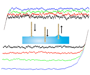
Motivated by the recent experiments in Guan et al. (Reference Guan, Wang, Charlaix and Tong2016a), we consider a capillary problem along a moving fibre. As shown in figure 4, we suppose a fibre is inserted in a liquid. When the fibre moves up and down, the contact line will recede and advance accordingly. We assume that the radius $r_0$ of the fibre is much smaller than the capillary length $l_c$. By the Young–Laplace equation, the radially symmetric liquid–vapour interface can be described by the following equation (see de Gennes et al. Reference de Gennes, Brochard-Wyart and Quere2003):

(2.17)\begin{equation} x=H(r)=h-r_0\cos\theta_a\ln\dfrac{r+\sqrt{r^{2}-r_0^{2}\cos^{2}\theta_a}}{r_0\cos\theta_a},\quad r\geq r_0. \end{equation}

Here, we assume the upper direction is the positive $x$-direction. There are two parameters, $h$ and $\theta _a$, in this equation. By the definition of the capillary length, we can assume that the interface intersects with the horizontal surface $x=0$ at $r=l_c$. Then we have

(2.18)\begin{equation} H(l_c)=0. \end{equation}

This gives a relation between $\theta _a$ and $h$, which is

(2.19)\begin{equation} h=r_0\cos\theta_a\ln\dfrac{l_c+\sqrt{l_c^{2}-r_0^{2}\cos^{2}\theta_a}}{r_0\cos\theta_a}. \end{equation}

Figure 4. Contact line motion on a moving fibre.

Notice that the $x$-coordinate of the contact line is given by

(2.20)\begin{equation} x_{ct}:=H(r_0)=h-r_0\cos\theta_a\ln\dfrac{1+\sin\theta_a}{\cos\theta_a}=r_0\cos\theta_a\ln\dfrac{l_c+\sqrt{l_c^{2}-r_0^{2}\cos^{2}\theta_a}}{r_0(1+\sin\theta_a)}. \end{equation}

Direct calculation gives

(2.21)\begin{equation} \dot{x}_{ct}=r_0 \mathcal{G}^{{-}1}_2(\theta_a)\dot{\theta}_a, \end{equation}

where

(2.22)\begin{equation} \mathcal{G}^{{-}1}_2(\theta_a)=r_0^{{-}1}\dfrac{\partial x_{ct}}{\partial\theta_a}\approx{-}\left( \sin\theta_a\ln\dfrac{2l_c}{r_0(1+\cos\theta_a)}+1-\sin\theta_a\right). \end{equation}

Equation (2.21) gives a relation between the time derivative of the contact line position and that of the dynamic contact angle.

Applying the boundary condition (2.6) to the relative velocity of the contact line $\dot {x}_{ct}-u_{wall}$, we obtain

(2.23)\begin{equation} \left(\alpha+ \dfrac{|\ln\zeta|}{\mathcal{F}_1(\theta_a)} \right)\dfrac{\mu}{\gamma}(\dot{x}_{ct}-u_{wall}) ={-} (\cos\theta_a-\cos\theta_Y). \end{equation}

The two equations compose a complete system for the capillary rising problem. They can be rewritten as

(2.24)\begin{equation} \left. \begin{aligned} \dot{\theta}_a & =\dfrac{\mathcal{G}_2(\theta)}{r_0}\left(-\left(\alpha+ \dfrac{|\ln\zeta|}{\mathcal{F}_1(\theta_a)}\right)^{{-}1}\dfrac{\gamma}{\mu}(\cos\theta_a-\cos\theta_Y)+u_{wall}\right),\\ \dot{x}_{ct} & ={-}\left(\alpha+ \dfrac{|\ln\zeta|}{\mathcal{F}_1(\theta_a)}\right)^{{-}1}\dfrac{\gamma}{\mu}(\cos\theta_a-\cos\theta_Y)+u_{wall}. \end{aligned} \right\} \end{equation}

This generalizes the formula given in Xu & Wang (Reference Xu and Wang2020). We would like to remark that for this problem we actually need to solve a three-dimensional two-phase Stokes system in a region around the fibre when we calculate the total viscous dissipation in the system. This may lead to a correction for the three-dimensional effect in the function $\mathcal {F}_1(\theta )$. Hereinafter, we ignore this effect for simplicity.

We can see that the ordinary differential systems (2.16) and (2.24) in the two examples have the same structure. They can be written as a unified form as follows:

(2.25)\begin{equation} \left. \begin{aligned} \dot{\theta}_a & =\dfrac{\mathcal{G}(\theta_a)}{l_0}\left(-\dfrac{\gamma}{\mu}\left(\alpha+ \dfrac{|\ln\zeta|}{\mathcal{F}_1(\theta_a)}\right)^{{-}1}(\cos\theta_a-\cos\theta_Y)+u_{wall}\right),\\ \dot{x}_{ct} & ={-} \dfrac{\gamma}{\mu}\left(\alpha+ \dfrac{|\ln\zeta|}{\mathcal{F}_1(\theta_a)}\right)^{{-}1}(\cos\theta_a-\cos\theta_Y)+u_{wall}. \end{aligned} \right\} \end{equation}

The second equation of (2.25) is due to the condition (2.7) where $\mathcal {F}_1(\theta _a)$ is given in (2.14). Since $\mathcal {F}_1(\theta _a)=\mathcal {F}(\theta _a,0)$, it corresponds to the case when ${\mu _B}/{\mu _A}=0$ (see (2.4)), i.e. a liquid–vapour system. In the first equation of (2.25), $l_0$ is a characteristic length and the function $\mathcal {G}(\theta _a)$ comes from the geometric set-up of a problem. Both $l_0$ and $\mathcal {G}(\theta _a)$ may change for different problems. Hereinafter, we will use (2.25) as a model problem to study the CAH for a liquid–vapour system on a chemically patterned surface.

3.1. Time averaging of the ODE system

We first introduce some properties satisfied by the dynamic factor $f$ and $g$

(3.4a,b)\begin{equation} f(\theta)\geq 0, f(0)=0;\quad -M\leq g(\theta) \leq{-}m, \end{equation}

for some positive numbers $m$ and $M$. In addition, we also assume that $f$ is monotonically increasing in the interval $[0,{\rm \pi} ]$. These conditions are quite general and are satisfied by the two examples in the previous section.

We assume that the substrate has periodic chemical patterns with period $\varepsilon$ so that Young's angle at the position $x$ satisfies $\hat {\theta }_Y(x)=\varphi ({x}/{\varepsilon })$, where $\varphi$ is a periodic continuously differentiable function with period 1. The minimum and maximum of $\varphi$ are $\theta _A$ and $\theta _B$, respectively, with $0<\theta _A<\theta _B<{\rm \pi}$. One example of such functions is

(3.5)\begin{equation} \varphi(z)=\dfrac{\theta_A+\theta_B}2+\dfrac{\theta_B-\theta_A}2\sin(2{\rm \pi} z). \end{equation}

In the following, we will use the method of averaging to derive the effective dynamics of the contact angle and contact line position. This method has been studied in detail (e.g. in Pavliotis & Stuart Reference Pavliotis and Stuart2008; E Reference E2011) and has been widely used in obtaining the effective boundary conditions (e.g. Miskis & Davis Reference Miskis and Davis1994).

We introduce the fast spatial variable $y={\hat {x}_{ct}}/{\varepsilon }$ and fast temporal variable $\tau ={t}/{\varepsilon }$. Consider the multiple scale asymptotic expansions

(3.6a,b)\begin{equation} \theta_a=\theta_0(t,\tau)+\varepsilon\theta_1(t,\tau)+\cdots,\quad y=y_0(t,\tau)+\varepsilon y_1(t,\tau)+\cdots. \end{equation}

Then the system of (3.2) can be rewritten as

(3.7a)\begin{align} &\dfrac 1{\varepsilon}\dfrac{\partial\theta_0}{\partial \tau}+\left(\dfrac{\partial\theta_0}{\partial t}+\dfrac{\partial\theta_1}{\partial \tau}\right)+\varepsilon\left(\dfrac{\partial\theta_1}{\partial t}+\dfrac{\partial\theta_2}{\partial \tau}\right)+\cdots\nonumber\\ &\quad =g(\theta_0+\varepsilon\theta_1+\cdots)\left(f(\theta_0+\varepsilon\theta_1+\cdots)(\cos\varphi(y_0+\varepsilon y_1+\cdots)\right.\nonumber\\ &\left.\qquad-\cos(\theta_0+\varepsilon\theta_1+\cdots))+v\right), \end{align}

(3.7b)\begin{align} &\dfrac 1{\varepsilon}\dfrac{\partial y_0}{\partial \tau}+\left(\dfrac{\partial y_0}{\partial t}+\dfrac{\partial y_1}{\partial \tau}\right)+\varepsilon\left(\dfrac{\partial y_1}{\partial t}+\dfrac{\partial y_2}{\partial \tau}\right)+\cdots\nonumber\\ &\quad =\dfrac{1}{\varepsilon}f(\theta_0+\varepsilon\theta_1+\cdots)(\cos\varphi(y_0+\varepsilon y_1+\cdots)-\cos(\theta_0+\varepsilon\theta_1+\cdots)). \end{align}

First-order equations in $O(1/{\varepsilon })$. We have the two equations in the fast time scale

(3.8)$$\begin{gather} \dfrac{\partial\theta_0}{\partial \tau}=0, \end{gather}$$

(3.9)$$\begin{gather}\dfrac{\partial y_0}{\partial \tau}=f(\theta_0)(\cos\varphi(y_0)-\cos\theta_0) . \end{gather}$$

The first equation implies that $\theta _0=\theta _0(t)$ is indeed a slow variable that does not depend on the fast time scale $\tau$. Then, for given $\theta _0$, the second equation is a simple ODE for $y_0$ with respect to $\tau$, that can be easily solved. We discuss its solution in two different cases for the parameter $\theta _0$.

In the first case when $\theta _0\in [\theta _A,\theta _B]$, for any given initial value for $y_0$, the solution of (3.9) approaches some equilibrium value $y_{0,\infty }$, which satisfies $\varphi (y_{0,\infty })=\theta _0$. By the phase plane analysis (see figure 5), we know that there are three types of equilibrium points: $y_{0,\infty }$ is asymptotically stable, semi-stable or unstable if $\varphi '(y_{0,\infty })>0$, $\varphi '(y_{0,\infty })=0$ or $\varphi '(y_{0,\infty })<0$, respectively. Every solution path must be attracted to either an asymptotically stable point or a semi-stable point, regardless of the initial value of $y_0$. For instance, if the initial value $y_0^{init}$ satisfies $\varphi (y_0^{init})<\theta _0$, then $y_0$ increases monotonically with $\tau$ until it reaches the nearest equilibrium point $y_{0,\infty }$ which is larger than $y_0^{init}$. This equilibrium point must satisfy $\varphi '(y_{0,\infty })\geqslant 0$ and thus becomes asymptotically stable or semi-stable. If the initial value $y_0^{init}$ satisfies $\varphi (y_0^{init})>\theta _0$, then $y_0$ decreases monotonically with $\tau$ until it reaches the nearest equilibrium point $y_{0,\infty }$ that is smaller than $y_0^{init}$. This equilibrium point must also satisfy $\varphi '(y_{0,\infty })\geqslant 0$ and thus becomes asymptotically stable or semi-stable.

Figure 5. Sketch of phase plane analysis for the ODEs (3.8) and (3.9). Here, $\theta _0$ is independent of $\tau$; $y_0$ increases when $\theta _0>\varphi (y_0)$ and $y_0$ decreases when $\theta _0<\varphi (y_0)$.

In the second case that $\theta _0>\theta _B$ or $\theta _0<\theta _A$, $\cos \varphi (y_0)-\cos \theta _0$ is either always positive or always negative. As a result, $y_0$ is monotonic in $\tau$ and diverges to $\pm \infty$ either increasingly or decreasingly. Moreover, using the method of separable variables, $y_0$ can be solved and represented implicitly as

(3.10)\begin{equation} Q(y_0(t,\tau),\theta_0)=Q(y_0(t,0),\theta_0)+\tau, \end{equation}

where

(3.11)\begin{equation} Q(z,\phi)=\int\dfrac{\mathrm{d}z}{f(\phi)(\cos\varphi(z)-\cos\phi)} \end{equation}

is monotonically increasing or decreasing in $z$ and thus can be inverted to give $y_0(t,\tau )$.

Second-order equations in $O(1)$. We consider the $O(1)$ equation for $\theta$, which is given by

(3.12)\begin{equation} \dfrac{\partial\theta_0}{\partial t}+\dfrac{\partial\theta_1}{\partial \tau}=g(\theta_0)\left(f(\theta_0)(\cos\varphi(y_0)-\cos\theta_0)+v\right). \end{equation}

We can assume that $\theta _1$ is of sublinear growth in $\tau$, i.e. there exists a constant $\alpha \in [0,1)$ such that $|\theta _1(t,\tau )|\leqslant C|\tau |^{\alpha }$ for some constant $C$ (see also E Reference E2011). Define the time averaging operator $\langle \cdot \rangle _\tau$ as

(3.13)\begin{equation} \langle F\rangle_\tau=\lim_{T\rightarrow\infty}\dfrac 1T\int_0^{T}F(\tau)\,\mathrm{d}\tau. \end{equation}

Then, applying this time averaging operator to (3.12) gives rise to

(3.14)\begin{equation} \dfrac{\partial\theta_0}{\partial t}=g(\theta_0)\left(\langle f(\theta_0)(\cos\varphi(y_0)-\cos\theta_0)\rangle_\tau+v\right), \end{equation}

where we have used the sublinearity of $\theta _1$ to eliminate $\langle {\partial \theta _1}/{\partial \tau }\rangle _\tau$.

From the previous analysis for the leading-order equations, $y_0$ is monotonic in $\tau$. Thus we can simplify the averaged term by using (3.9),

(3.15)\begin{equation} \langle f(\theta_0)(\cos\varphi(y_0)-\cos\theta_0)\rangle_\tau=\lim_{T\rightarrow\infty}\dfrac 1T\int_0^{T}\dfrac{\partial y_0}{\partial \tau}\,\mathrm{d}\tau=\lim_{T\rightarrow\infty}\dfrac{y_0(t,T)-y_0(t,0)}T. \end{equation}

We discuss the limit on the right-hand side for different cases on $\theta _0$. In the first case that $\theta _0\in [\theta _A,\theta _B]$, this limit is zero since every solution path $y(t,\cdot )$ converges to an asymptotically stable or semi-stable equilibrium point (by the analysis for the leading-order equations). In the second case that $\theta _0>\theta _B$ or $\theta _0<\theta _A$, we shall show that this limit is

(3.16)\begin{equation} \left(\int_0^{1}\dfrac{\mathrm{d}z}{f(\theta_0)(\cos\varphi(z)-\cos\theta_0)}\right)^{{-}1}, \end{equation}

the harmonic average of $f(\theta _0)(\cos \varphi (z)-\cos \theta _0)$ over $z\in [0,1]$.

The argument for the second case is as follows. Let

(3.17)\begin{equation} b=\int_0^{1}\dfrac{\mathrm{d}z}{f(\theta_0)(\cos\varphi(z)-\cos\theta_0)}=\dfrac{1}{f(\theta_0)} \int_0^{1}\dfrac{\mathrm{d}z}{(\cos\varphi(z)-\cos\theta_0)}. \end{equation}

From (3.10) we know that if $\tau =nb$ for any integer $n$, then

(3.18)\begin{equation} y_0(t,\tau)-y_0(t,0)=n. \end{equation}

Writing $T=nb+a$ with $n=\lfloor T/b\rfloor$ (the largest integer no greater than $T/b$) and $0\leqslant a< b$, and letting $n\rightarrow \infty$, we have

(3.19)\begin{equation} \lim_{T\rightarrow\infty}\dfrac{y_0(t,T)-y_0(t,0)}T=b^{{-}1}. \end{equation}

This implies that $\langle f(\theta _0)(\cos \varphi (y_0)-\cos \theta _0)\rangle _\tau$ is exactly equal to the harmonic average of $f(\theta _0)(\cos \varphi (z)-\cos \theta _0)$ over a period $[0,1]$.

By the above calculations, (3.14) is reduced to

(3.20)\begin{equation} \dfrac{{\rm d} \theta_0}{{\rm d} t}=\begin{cases}g(\theta_0)v, & \theta_0\in[\theta_A,\theta_B];\\ g(\theta_0)(b^{{-}1}+v), & \theta_0>\theta_B\ {\rm or}\ \theta_0<\theta_A.\end{cases} \end{equation}

By this equation, we can discuss the dynamics for the slow variable $\hat {x}_{ct}$. As $\varepsilon \rightarrow 0$ we have

(3.21)\begin{align} \dfrac{\mathrm{d}\hat{x}_{ct}}{\mathrm{d}t}&=\dfrac{\partial y_0}{\partial \tau}+\varepsilon\left(\dfrac{\partial y_0}{\partial t}+\dfrac{\partial y_1}{\partial \tau}\right)+O(\varepsilon^{2})\nonumber\\ &\sim f(\theta_0)(\cos\varphi(y_0)-\cos\theta_0)+O(\varepsilon). \end{align}

On application of the time averaging operator $\langle \cdot \rangle _\tau$, the leading order of $\hat {x}_{ct}$ satisfies

(3.22)\begin{equation} \dfrac{\mathrm{d}\langle \hat{x}_{ct,0}\rangle_{\tau}}{\mathrm{d}t}= \langle f(\theta_0)(\cos\varphi(y_0)-\cos\theta_0)\rangle_\tau=\begin{cases}0, & \theta_0\in[\theta_A,\theta_B],\\ b^{{-}1}, & \theta_0>\theta_B\ {\rm or}\ \theta_0<\theta_A.\end{cases} \end{equation}

We introduce the average of the contact angle and the contact point position such that

(3.23a,b)\begin{equation} {\varTheta}_a:=\langle \theta_0\rangle_{\tau}=\theta_0,\quad \text{and}\quad \hat{X}_{ct}:=\langle \hat{x}_{ct,0}\rangle_{\tau}. \end{equation}

The above analysis can be summarized as follows. In the first case that $\theta _A\leqslant {\varTheta }_a \leqslant \theta _B$, the averaged equations are

(3.24a)$$\begin{gather} \dot{\varTheta}_a=g(\varTheta_a)v, \end{gather}$$

(3.24b)$$\begin{gather}\dot{\hat{X}}_{ct}=0. \end{gather}$$

In the second case that ${\varTheta }_a >\theta _B$ or ${\varTheta }_a<\theta _A$, the averaged equations are

(3.25a)$$\begin{gather} \dot{\varTheta}_a=g(\varTheta_a)\left(f(\varTheta_a)\left(\int_0^{1}\dfrac{\mathrm{d}z}{\cos\varphi(z)-\cos\varTheta_a}\right)^{{-}1}+v\right), \end{gather}$$

(3.25b)$$\begin{gather}\dot{\hat{X}}_{ct}=f(\varTheta_a)\left(\int_0^{1}\dfrac{\mathrm{d}z}{\cos\varphi(z)-\cos\varTheta_a}\right)^{{-}1}. \end{gather}$$

3.2. The effective contact angles

Based on the above analysis, we can make a prediction for the averaged apparent contact angle $\varTheta _a$ and the averaged contact line motion $\dot {\hat {X}}_{ct}$. This will lead to the formula for the effective advancing and receding contact angles when the contact line moves on a chemically patterned surface.

First consider the case $v>0$, i.e. the wall moves in the positive direction. This corresponds to a receding contact line, since the fluid moves to the negative direction relative to the substrate. We discuss three possible stages while leaving the details to Appendix C:

1. (i) When the initial value of the contact angle $\varTheta _a$ lies in the regime $(\theta _B,{\rm \pi} ]$, the averaged contact line dynamics follows (3.25). In this stage, the effective contact angle $\varTheta _a$ decreases towards $\theta _B$ exponentially fast. Moreover, the effective contact line position $\hat {X}_{ct}$ moves in the positive direction. This first stage is indeed a transient stage.

2. (ii) When the contact angle $\varTheta _a$ reaches $\theta _B$, the averaged dynamics switches to (3.24). The effective contact angle $\varTheta _a$ continues decreasing until it reaches $\theta _A$. However, the effective contact line position $\hat {X}_{ct}$ remains unchanged.

3. (iii) When the contact angle $\varTheta _a$ attains $\theta _A$, the averaged dynamics switches back to (3.25). In this situation, the effective contact angle $\varTheta _a$ decreases until it eventually arrives at a stable steady state $\varTheta ^{*}<\theta _A$. The steady state $\varTheta ^{*}$ satisfies

   (3.26)\begin{equation} f(\varTheta^{*})\left(\int_0^{1}\dfrac{\mathrm{d}z}{\cos\varphi(z)-\cos\varTheta^{*}}\right)^{{-}1}+v=0. \end{equation}
   When $\varTheta _a$ attains $\varTheta ^{*}$, the effective contact line position $\hat {X}_{ct}$ moves in the negative direction at a constant velocity equal to $-v$.

If the initial contact angle lies in the regime $[\theta _A,\theta _B]$ or $[0,\theta _A)$, the above three-stage dynamics may be reduced to a two-stage process or only one stage. In all these situations, $\varTheta _a$ always reaches the equilibrium contact angle $\varTheta ^{*}$. Meanwhile, the average contact line position ${\hat {X}}_{ct}$ finally moves with a constant negative velocity $-v$. Notice that it is the actual contact line position on the solid wall. The equilibrium contact angle $\varTheta ^{*}$ is actually the effective receding contact angle, which is denoted by $\varTheta ^{*}=\varTheta ^{*}(v)$ as a function of $v>0$.

In the case of $v<0$, a similar analysis can be made to predict the dynamics of the effective advancing contact angle, with the corresponding velocities of opposite signs. The effective contact angle $\varTheta _a$ eventually arrives at a steady state $\varTheta ^{*}$, which also satisfies (3.26); and the actual contact line position $\hat{X}_{ct}$ moves with a constant positive velocity $-v$. The final steady state $\varTheta ^{*}$ is called the effective advancing contact angle, which is also denoted by $\varTheta ^{*}=\varTheta ^{*}(v)$ for $v<0$.

As an interesting but important fact, we remark that: the effective advancing contact angle $\varTheta ^{*}(v)>\theta _B$ with $v<0$, and it approaches $\theta _B$ as $v$ increases to zero; the effective receding contact angle $\varTheta ^{*}(v)<\theta _A$ with $v>0$, and it approaches $\theta _A$ as $v$ decreases to zero. When $v=0$, the contact line can be pinned for any contact angle between $\theta _A$ and $\theta _B$. Similar ideas have been investigated in many phenomenological moving contact line models in the study of CAH (Prabhala, Panchagnula & Vedantam Reference Prabhala, Panchagnula and Vedantam2013; Yue Reference Yue2020).

In summary, depending on the initial value of the contact angle, the averaged dynamics of the contact line and the contact angle can be characterized by a process with at most three stages as described above. In any cases, one approaches to a steady state where the effective advancing angle or receding angle does not change any more. The effective contact angles are given by the (3.26). It is worth noting that the final effective advancing and receding contact angles only depend on the dynamic factor $f(\theta _a)$ and the dragging velocity $v$. The geometric factor $g(\theta _a)$ only affects the dynamic process that how $\varTheta _a$ approaches the effective advancing and receding contact angles. The above results are numerically validated in § 5.

5.1. Verification of the analysis

We first consider the case of a two-dimensional microscopic channel where the geometric factor is given by $g(\theta )={4\mathcal {G}_1(\theta )}$ and the dynamic factor is given by $f(\theta _a)={\mathcal {F}_1(\theta _a)}/{|\ln \zeta |}$. We neglect the contact line friction ($\alpha =0$) for simplicity. We use the sine pattern for $\varphi (y)$ with the two extrema being $\theta _A=60^{\circ }$ and $\theta _B=120^{\circ }$. The cutoff parameter is set to be $\zeta =100$.

Figure 8 shows the evolutional behaviour of the dynamic contact angle $\theta _a$ and the contact line position $\hat {x}_{ct}$ modelled by (3.2) with different periods $\varepsilon =10^{-1}, 10^{-2}$ and $10^{-3}$. The dimensionless velocity is ${v}=0.01$, and the initial contact angle is $\theta _{init}=150^{\circ }$. It shows a clear three-stage process.

Figure 8. Receding dynamics for $\varepsilon =0.1, 0.01, 0.001$ and ${v}=0.01$ given $\theta _A=60^{\circ }$ and $\theta _B=120^{\circ }$. (a) Dynamical contact angle starting from $\theta _{init}=150^{\circ }$. (b) The contact line position starting from $\hat {x}_{ct}=0$.

1. (i) In the first stage, since the initial contact angle is greater than $\theta _B=120^{\circ }$ and the wall velocity is positive, the averaged dynamics (3.25) predicts that the contact line $\hat {x}_{ct}$ moves to the positive direction and the contact angle $\theta _a$ decreases towards $\theta _B$. This is consistent with the numerical results of the original dynamics (3.2) (shown by red curves), in particular for small $\varepsilon$ as depicted by the solid blue and black curves. Moreover, this stage is very short and thus is transient.

2. (ii) When $\theta _a$ is around $\theta _B=120^{\circ }$, the second-stage dynamics emerges. The contact line moves very slowly as if it stays almost unchanged, but the contact angle continues to recede. This behaviour is consistent with the prediction by the averaged dynamics (3.24).

3. (iii) As the receding angle achieves some value around $\theta _A=60^{\circ }$, the dynamical process goes into the third stage. The contact angle oscillates around the effective receding contact angle given by (3.26). There are also oscillations for the contact line position $\hat {x}_{ct}$. However, the averaged position of the contact line increases linearly with respect to the time.

In the third stage, the contact line moves to the negative direction relative to the wall with a stick-slip effect. Take the $\varepsilon =0.01$ case for example (in the zoom-in plot). As the contact angle achieves approximately $57.5^{\circ }$, the contact line starts to move fast (e.g. the zoom-in plot of the $\varepsilon =0.01$ curve when $t=9.5$). This fast movement of $\hat {x}_{ct}$ in turn leads to a fast increase of $\theta _a$ until $\theta _a$ arrives at approximately $62^{\circ }$. This is the slip behaviour of the contact line. When $\theta _a$ is around $62^{\circ }$, the deviation of $\theta _a$ from $\varphi (\hat {x}_{ct})$ is small so that the contact line moves very slowly as if it sticks there (e.g. $\hat {x}_{ct}\approx 0.047$ in the zoom-in plot of the $\varepsilon =0.01$ curve). The angle $\theta _a$ decreases slowly towards $57.5^{\circ }$ and another stick-slip period follows. Both the oscillation of the contact angle and the stick-slip of the contact line position share the same period proportional to $\varepsilon$. The stick-slip motion has also been discussed in detail in Xu & Wang (Reference Xu and Wang2020).

Figure 8 also shows that the dynamics of the contact angle and the contact line position converges to the averaged dynamics (red curves) modelled by (3.24) and (3.25) as the period $\varepsilon$ decreases. When $\varepsilon =10^{-3}$, the differences between the original dynamics and the averaged dynamics is quite small.

When $v$ is negative, the situation is similar to that shown in figure 8. In this case, one will observe the effective advancing contact angle in the third stage instead (also see the plots in figure 9). For the other choices of $\theta _A$, $\theta _B$ and initial angle $\theta _{init}$, the numerical results are also similar except that the three-stage behaviour may be replaced by a two-stage process or a one-stage process depending on whether $\theta _{init}$ is inside or outside $[\theta _A,\theta _B]$.

Figure 9. Advancing and receding dynamics for $\varepsilon =0.01$ and ${v}=\pm 0.02,\pm 0.01,\pm 0.005$ given $\theta _A=60^{\circ }$ and $\theta _B=120^{\circ }$. (a) Dynamical contact angle starting from $\theta _{init}=100^{\circ }$. (b) The contact line position starting from $0$. From top to bottom, the solid curves represent the contact angle and contact line motion in the original dynamics. The dashed curves are the corresponding averaged dynamics.

Figure 9 shows the effect of velocity $v$ on the dynamics. In these experiments, we fix $\varepsilon =0.01$, $\theta _{init}=100^{\circ }$ and vary the dimensionless velocity ${v}$ from 0.02 to -0.02. As shown by the bottom three groups of curves in figure 9, when ${v}>0$, the contact angle $\theta _a$ decreases towards the receding angle and the contact line position $\hat {x}_{ct}$ moves to the negative direction. In the stick-slip stage, the effective contact line velocity in the averaged dynamics is exactly equal to the wall velocity ${v}$. The effective receding angle also depends on ${v}$. As $|{v}|$ becomes smaller, the effective receding angle is closer to $\theta _A=60^{\circ }$ from below. In the case ${v}<0$, the advancing dynamics is observed and $\theta _a$ increases until it starts to oscillate around the effect advancing angle. Then, $\hat {x}_{ct}$ moves to the positive direction with an averaged velocity equal to ${v}$. As $|{v}|$ becomes smaller, the effective advancing angle is closer to $\theta _B=120^{\circ }$ from above. This validates our analysis in § 3.1. Moreover, the sensitivities of the effective receding and advancing contact angles to $|{v}|$ are different and asymmetric in this case.

Finally, we will study the effect of the geometric factor $g(\theta _a)$. We solve the problem (3.2) for two different choices of $g$, which correspond to the moving contact line problems in a microscopic channel ($g=4\mathcal {G}_1$) and on a moving fibre ($g=4\mathcal {G}_2$). Figure 10 shows the dynamics of the advancing and receding angles. It is clear that the geometric factor affects the dynamic process, especially the first two stages. The contact angle approaches its equilibrium value in the micro-channel case much faster than it does in the moving fibre case. However, the effective advancing and receding angles are the same in the two cases and they only depend on the dynamic factor $f(\theta _a)$, as shown by (3.26).

Figure 10. Advancing and receding dynamics for $\varepsilon =0.01$ and ${v}=\pm 0.01$ given $\theta _A=60^{\circ }$ and $\theta _B=120^{\circ }$. (a) Dynamical contact angle starting from $\theta _{init}=100^{\circ }$. (b) The contact line position starting from $0$. From top to bottom, the solid curves represent the contact angle and contact line dynamics with respect to ${v}=-0.01$ and ${v}=0.01$. Black curves show the dynamics in the case of a fibre while blue curves show the dynamics in the case of a microscopic channel. The dashed curves are the corresponding averaged dynamics.

5.2. Comparison with experimental results

In this subsection, we will use our model and analysis to explain the experimental results of Guan et al. (Reference Guan, Wang, Charlaix and Tong2016a,Reference Guan, Wang, Charlaix and Tongb). There, the dynamic CAH is observed by careful design of physical experiments. A very thin glass fibre with an inhomogeneous surface is inserted into a liquid reservoir. The fibre moves up and down so that a contact line moves on its surface. The capillary forces on the fibre are measured by atomic force microscopy (AFM) and the effective contact angles are computed. Several liquids with different surface tensions, viscosities and equilibrium angles are tested in their experiments. Many interesting phenomena are observed in the experiments. It is found that the dependence of the advancing and receding contact angles on the fibre velocity is not unified (see figure 6 in Guan et al. Reference Guan, Wang, Charlaix and Tong2016b). In some cases (e.g. the water–air system), the dependence of the advancing and receding contact angles on the velocity is very asymmetric. In some cases (e.g. the octanol–air system), this dependence seems symmetric. In some other cases (e.g. the FC77–air system), the advancing and receding contact angles are all very small and close to each other.

To compare with the experiments, we use the reduced model (2.24) which is an approximation for the problem in Guan et al. (Reference Guan, Wang, Charlaix and Tong2016b). The radius of the fibre is $r_0=1.1\,\mathrm {\mu } \textrm {m}$ which is consistent with the experiment. We suppose the surface of the fibre is composed of two different materials $A$ and $B$ with different Young's angles $\theta _A$ and $\theta _B$. On the surface, the pattern of the Young's angle $\varphi (z)$ is a piecewise constant periodic function with $\varphi _{\chi }(z)=\theta _A$ if $0\leqslant z<\chi$ and $\varphi _{\chi }(z)=\theta _B$ if $\chi \leqslant z<1$, where $\chi$ is the percentage of material $A$ in a period. For the convenience in numerical computations, we smooth this discontinuous pattern by a hyperbolic tangent function

(5.1)\begin{equation} \varphi_{\chi}^{\delta}(z)=\dfrac{\theta_A+\theta_B}{2}+\dfrac{\theta_B-\theta_A}{2}\tanh\left(\dfrac{\sin(2{\rm \pi} z)-\sin(\chi-1/2){\rm \pi}}{\delta}\right), \end{equation}

where $\delta \ll 1$ is chosen to control the thickness of the smooth transition between two patterns. We use $\varphi _{\chi }^{\delta }$ in our simulations. Here, $\theta _A$ and $\theta _B$ can be chosen approximately according to the receding and advancing contact angles in the experiments with the smallest moving speed. We choose the fraction $\chi$ and the dimensionless friction coefficient $\alpha$ as fitting parameters. The dimensionless wall velocity is represented by $v={\mu u_{wall}}/{\gamma }$, where the fibre speed $|u_{wall}|$ is suggested by the experiments as $2\,\mathrm {\mu } \textrm {m}\,\textrm {s}^{-1}, 5\,\mathrm {\mu } \textrm {m}\,\textrm {s}^{-1}, 20\,\mathrm {\mu } \textrm {m}\,\textrm {s}^{-1}$ and $50\,\mathrm {\mu } \textrm {m}\,\textrm {s}^{-1}$. We refer to table 1 of Guan et al. (Reference Guan, Wang, Charlaix and Tong2016b) for the material properties, especially the surface tension $\gamma$ and the viscosity $\mu$. Since the capillary lengths of the materials under consideration have the range 0.86–2.71 mm, we choose it to be $l_c=1$mm. The logarithm of the cutoff parameter is fixed at $\ln \zeta =10$. As we observe in the numerical experiments, the variation of $\ln \zeta$ in its reasonable regime (of order $O(10)$) does not affect the results too much.

The numerical results are given in figure 11. We could see that the dependence of the CAH on the capillary number is not unified. For all the four cases, the advancing and receding contact angles and their dependence on the wall velocity are similar to those in the experiments in Guan et al. (Reference Guan, Wang, Charlaix and Tong2016a,Reference Guan, Wang, Charlaix and Tongb). The numerical results also agree with the discussions in § 4.1 based on the formula (3.26) of the effective contact angle. This also indicates that the experimental observations may be understood from our theoretical analysis in § 3, especially (3.26) on the effective contact angles. There we show that effective advancing and receding contact angles depend on the capillary number, the friction coefficient, the Young's angles of the inhomogeneous substrate and also the spatial distributions of the patterns. All these parameters have important impacts and the interplay among them gives rise to very complicated experimental phenomena.

Figure 11. Dependence of CAH on different wall speeds. The dimensional period of the chemical pattern is set to be $\varepsilon =0.05\,\mathrm {\mu }$m. (a) Water–air, $\theta _A=105^{\circ }$, $\theta _B=115^{\circ }$, $\alpha =4\times 10^{5}$ and $\chi =0.9$. (b) Octanol–air, $\theta _A=45^{\circ }$, $\theta _B=60^{\circ }$, $\alpha =1\times 10^{4}$ and $\chi =0.4$. (c) Decane–air, $\theta _A=43^{\circ }$, $\theta _B=63^{\circ }$, $\alpha =5\times 10^{4}$ and $\chi =0.9$. (d) FC77–air, $\theta _A=13^{\circ }$, $\theta _B=14^{\circ }$, $\alpha =1\times 10^{3}$ and $\chi =0.4$. The black, red, green and blue curves represent the results with fibre speeds of $|u_{wall}|=2\,\mathrm {\mu }$m, $5\,\mathrm {\mu }$m, $20\,\mathrm {\mu }$m and $50\,\mathrm {\mu }$m, respectively.

In real experiments, there are always thermal noises which affect the dynamics of the contact line. To make the numerical results more comparable to the experiments, we add a stochastic force in (2.7) to model other non-deterministic effects, e.g. thermal noises. The resulting stochastic system for the apparent contact angle $\theta _d$ and contact line position $\hat {x}_{ct}$ reads

(5.2)\begin{equation} \left. \begin{aligned} \dot{\theta}_a & =g(\theta_a)(f(\theta_a)(\cos\hat{\theta}_Y(\hat{x}_{ct})-\cos\theta_a+\sigma\dot{W})+v),\\ \dot{\hat{x}}_{ct} & = f(\theta_a)(\cos\hat{\theta}_Y(\hat{x}_{ct})-\cos\theta_a+\sigma\dot{W}). \end{aligned} \right\} \end{equation}

This system of equations should be understood in the Itô sense. Since the contact angle and the contact line position are linked by the kinematic constraint (e.g. (2.12) and (2.21)) through the geometric factor $g(\theta _a)$, they are driven by the same Brownian motion $W(t)$. We choose the noise level to be small so that it does not affect the dynamics too much. We then numerically solve (5.2) for one sample path using the Euler–Maruyama scheme. Numerical results by solving the stochastic equation (5.2) are shown in figure 12. We could see a similar velocity dependence of the CAH as that in figure 11 in the deterministic case. Moreover, the dynamic behaviours fit well with the experiments for all the four cases, i.e. the water–air, octanol–air, decane–air and FC77–air systems (Guan et al. Reference Guan, Wang, Charlaix and Tong2016b).

Figure 12. Dependence of CAH on different wall speeds in the presence of noise. The dimensional period of the chemical pattern is set to $\varepsilon =0.05\,\mathrm {\mu }$m. The noise level $\sigma$ is chosen case by case without affecting the effective advancing and receding angles. (a) Water–air, $\theta _A=105^{\circ }$, $\theta _B=115^{\circ }$, $\alpha =4\times 10^{5}$, $\chi =0.9$ and $\sigma =0.1$. (b) Octanol–air, $\theta _A=45^{\circ }$, $\theta _B=60^{\circ }$, $\alpha =1\times 10^{4}$, $\chi =0.4$ and $\sigma =0.02$. (c) Decane–air, $\theta _A=43^{\circ }$, $\theta _B=63^{\circ }$, $\alpha =5\times 10^{4}$, $\chi =0.9$ and $\sigma =0.03$. (d) FC77–air, $\theta _A=13^{\circ }$, $\theta _B=14^{\circ }$, $\alpha =1\times 10^{3}$, $\chi =0.4$ and $\sigma =0.002$. The black, red, green and blue curves represent the results with fibre speeds at $|u_{wall}|=2\,\mathrm {\mu }$m, $5\,\mathrm {\mu }$m, $20\,\mathrm {\mu }$m and $50\,\mathrm {\mu }$m, respectively.

In the end, we would like to remark that the previous comparisons with experiments are almost quantitative, since the fibre velocities are chosen to be the same as in the experiments. Here, we choose the fraction $\chi$ of the chemical pattern as a fitting parameter. The reason can be understood as follows. In our simplified model, we assume that the contact line on the fibre is circular and the liquid–air interface is axisymmetric. This assumption does not hold in real experiments, where the chemical inhomogeneity is very complex on the fibre surface. The relaxation behaviour of the contact line is much more complicated than that in our model. Although it is possible to use a circular curve to approximate the contact line on such surfaces by homogenization (Joanny & De Gennes Reference Joanny and De Gennes1984; Xu Reference Xu2016), the effective pattern in the axial direction might be different for different liquids even on the same substrate. This is due to the fact that the correlation length of the oscillating contact line can be very different (Golestanian & Raphaël Reference Golestanian and Raphaël2003; Golestanian Reference Golestanian2004). Actually, this can be seen from the experiments in Guan et al. (Reference Guan, Wang, Charlaix and Tong2016b), where the periods of the effective patterns seem very different for different fluids. The characterization of dynamic CAH on general surfaces with chemical and geometrical roughness in three dimensions is very interesting and will be left for future work.