2.1 Computational fluid dynamic simulation disk design

Prior to fabricating the disk, computational fluid dynamic (CFD) simulations were performed to aid in the design of the suction system. The objective was to design a system that could produce a region of uniform wall suction around the location of $Re_{c_{A}}$ . The details of the simulation are presented in appendix B.

The simulation was performed for the disk spinning at 1500 r.p.m., corresponding to ${\it\omega}=157.1~\text{s}^{-1}$ . This was an upper limit for the rotating disk set-up at which a suction parameter of $a=0.4$ located the $Re_{c_{A}}=803$ over the suction portion of the disk, at $r_{c_{A}}=25.5~\text{cm}$ . In this case, for $a=0.4$ , $v_{z_{0}}=-2~\text{cm}~\text{s}^{-1}$ . This r.p.m. condition was meant to represent a worst case with regard to any induced flow within the enclosure that would influence the distribution of suction through the holes in the disk.

A first validation of the rotating disk simulation simply involved comparing the resulting boundary layer mean velocity profiles against those of the exact solution for a solid disk, without through holes. The result is shown in figure 3, where the symbols represent the simulation results and the curves represent the exact solution corresponding to the standard normalized radial, $H$ , tangential (azimuthal), $F$ , and axial, $G$ , velocity components. The simulation results and exact solution were found to agree very well.

Figure 3. Validation of simulation boundary layer profiles against the exact solution for a solid rotating disk.

Following this validation with a solid disk, the simulation was used to investigate the sensitivity of the radial pressure gradient over the measurement side of the disk to the suction enclosure dimension. The disk in the simulation included the through holes between the measurement and the underside of the disk. The wire mesh covering over the holes was not included in this simulation. Two different enclosure sizes were investigated: the first was 5 ft $\times$ 5 ft, which matched that of Gregory & Walker (Reference Gregory and Walker1960), and the second was twice as large (10 ft $\times$ 10 ft). Both enclosures had a depth of 15 in. The initial static pressure in the enclosure was set to be atmospheric. The results are shown in figure 4. The rotation of the disk caused a lowering of the pressure in the enclosure which resulted in air being drawn through the holes from the measurement side of the disk. The wall-normal velocity normalized by the maximum value, $v_{z}/v_{z_{max}}$ , is shown as a function of the radial position on the disk. The simulation indicates that doubling the size of the enclosure below the disk would not change the radial uniformity by an appreciable amount. As a result, the smaller enclosure size was used in the experiment.

Figure 4. Simulation results of the effect of the under-disk enclosure size on the radial distribution of wall-normal velocity through the holes through the disk with rotation. The wire mesh covering was not included.

As indicated previously, Gregory & Walker (Reference Gregory and Walker1960) had used a porous wire mesh to cover the suction holes in the disk. The simulation was then used to investigate this aspect, in both the necessity and the degree of the added pressure drop over the holes. Figure 5 shows the simulation results without the holes covered. This is for the smaller 5 ft planform enclosure, and without active suction. The simulation indicates fairly large passive suction with velocities ranging from 2 to $4~\text{m}~\text{s}^{-1}$ . In addition, the simulation reveals some passive blowing that occurs in the radially inboard side of the holes through the disk. Detailed analysis of this indicated a small separation bubble near the top edge of the holes.

The results in figure 6 are for the same conditions as figure 5 except for the addition of a pressure drop corresponding to a pressed wire mesh screen with the characteristics of LFM-25 in table 1 placed over the holes. Immediately apparent in the results is a two-order-of-magnitude reduction of the passive suction velocity with the addition of the pressure drop producing mesh covering. In addition, except at the most outboard location, there is no passive blowing through the holes. This justifies the use of the porous mesh covering by Gregory & Walker (Reference Gregory and Walker1960).

In this simulation, the target $v_{z_{0}}=-2~\text{cm}~\text{s}^{-1}$ resulted in $Re_{c_{A}}=803$ . The simulation indicated that that suction velocity was achievable, and that the suction velocity was relatively constant near the target radius. This was the final step in solidifying the design of the rotating disk with wall suction set-up.

Figure 5. Radial distribution of wall-normal velocity at the disk surface, with rotation and without active suction or a wire mesh covering.

Figure 6. Radial distribution of wall-normal velocity at the disk surface, with rotation, a wire mesh covering and suction with $a=0.4$ .

3.1 Basic flow with suction

The challenge in the experiment was to have surfaces on the measurement side of the disk that were (1) porous, (2) smooth and (3) uniform in thickness. As discussed in the introduction, the stationary cross-flow modes are highly receptive to surface roughness. Wall suction, which thins the boundary layer, makes the requirement on achieving a smooth surface critically important. Furthermore, wall suction increases $Re_{c_{A}}$ , meaning that laminar flow needs to be maintained out to larger radii. The uniformity of the thickness of the porous sheet covering the disk is important to allow hot-wire measurements as close as possible to the disk surface. The requirement on the thickness uniformity was a deviation of less than 0.13 mm in order to resolve the peak in the cross-flow mode wall-normal eigenfunction that occurs at $z^{\ast }\simeq 1.5$ .

A number of porous measurement surfaces had been investigated. They consisted of an uncovered compressed wire mesh, the same compressed wire mesh with two different stretched fabric coverings, and the same compressed wire mesh that was covered by a 1.6 mm thick sheet of porous high-density polyethylene. The polyethylene sheet had a $20~{\rm\mu}\text{m}$ pore size. The uncovered compressed wire mesh surface was comparable to one of the surfaces used by Gregory & Walker (Reference Gregory and Walker1960).

These different surfaces were examined in terms of (1) the ability to match theoretical wall-normal velocity profiles with different suction parameters and (2) the ability to maintain laminar flow out to the vicinity of the radius location of $Re_{c_{A}}$ . Of these, the second became the greater challenge, since even minute surface roughness could result in dominant stationary cross-flow modes that would lead to turbulent transition inboard of the $Re_{c_{A}}$ location. This is presumed to be what occurred in the suction experiments of Gregory & Walker (Reference Gregory and Walker1960), in which transition was reported to occur well inboard of what would have been $Re_{c_{A}}$ for their $a=0.4$ suction parameter.

Of the four surfaces examined, only the polyethylene sheet was smooth enough to maintain laminar flow out to a radius close to $Re_{c_{A}}=650$ with the desired suction parameter of $a=0.2$ . Unlike the stretched fabric coverings, the polyethylene sheet was semi-rigid and therefore could not be stretched over the disk surface. Instead, the sheet was bonded to the solid centre portion of the disk, and clamped by a ring at the outer edge of the disk. The outer clamping ring was the same as that shown with the fabric covering in figure 23(d). An issue with the polyethylene sheet was that it was not precisely uniform in thickness. As a result, there was a slight once-per-revolution waviness of the surface of 0.08 mm. This did not appear to affect the character of the cross-flow instability. However, it limited how close to the disk surface the hot wire could be traversed. In general, measurements down to the location of the maximum azimuthal velocity fluctuation, $z^{\ast }\simeq 1.5$ , were achievable.

Mean azimuthal velocity measurements were performed over the polyethylene sheet that covered the disk in order to compare them with the theoretical velocity profile, as well as previous measurements of Gregory & Walker (Reference Gregory and Walker1960). In order to compare with Gregory and Walker, the measurements were taken at the location on the disk where $Re=319$ . To accomplish this, the disk r.p.m. was reduced to 600, which corresponded to ${\it\omega}=62.8~\text{s}^{-1}$ . The results are shown in figure 7 for a desired $a=0.2$ suction parameter. The wall coordinate and mean azimuthal velocity are presented in similarity form, $z^{\ast }=z({\it\omega}/{\it\nu})^{1/2}$ and $\overline{U}_{{\it\theta}}/(r{\it\omega})$ respectively. The theoretical mean azimuthal velocity profiles are shown by the different curves corresponding to different suction parameters. These were found by the solution of the four ordinary differential equations governing the viscous mean flow over a rotating disk in similarity variables (Schlichting Reference Schlichting1968), namely

where

and ${\it\zeta}=z({\it\omega}/{\it\nu})^{1/2}$ . The standard boundary conditions were used, namely

The equations were solved using a Runge–Kutta–Gill integration between collocation points. To facilitate this, values for $F^{\prime }(0)$ and $G^{\prime }(0)$ from Dhanak (Reference Dhanak1992) were used based on the different suction parameters, $a$ .

Figure 7. Wall-normal profiles of the azimuthal velocity at $Re=319$ for ${\it\omega}=62.8~\text{s}^{-1}$ and $a=0.2$ .

For the present results at $Re=319$ in figure 7, the measured azimuthal velocity profile follows the shape of the theoretical profile for the intended $a=0.2$ reasonably well. We note that some points fall between the $a=0.2$ and $a=0$ theoretical profiles. As is evident, the differences between the two theoretical profiles, as well as that for $a=0.4$ , are small. We did our best to fine tune the wall suction as much as possible to be closest to the $a=0.2$ profile. The unavoidable azimuthal thickness variation in the polyethylene sheet covering the disk prevented measurements closer to the disk surface. The horizontal line marks the lowest height before which the hot wire would touch some part of the disk surface. The comparable measured azimuthal velocity profiles of Gregory & Walker (Reference Gregory and Walker1960) were observed to deviate from the theoretical profile closer to the disk surface. They observed that the profiles were fuller, indicating a lower value of the shape factor for the azimuthal component. At least in the limited profile extent of the present measurements, this was not the case.

The measured mean azimuthal velocity profiles at the radial locations corresponding to $518\leqslant Re\leqslant 620$ for the rotating disk conditions that were listed in the table in figure 1 are shown in figure 8. The radius $Re=518$ is significant because that was the location at which the air-pulse disturbances were introduced. The radius $Re=620$ is slightly inboard of $Re_{c_{A}}=650$ which was expected with $a=0.2$ . Ideally, we wanted to achieve a uniform suction parameter over all of the disk. However, this proved to be difficult as the r.p.m. of the disk was increased. The simulation results that were shown in figure 6, however, indicated that the change with radius would asymptote in the vicinity of $Re_{c_{A}}$ . This was found to be the case, whereby the velocity profiles stopped changing with increasing radius ( $Re$ ), and converged to a single profile for $Re\geqslant 611$ . The process of setting the wall suction conditions was then to adjust the pressure in the enclosure below the disk so that the mean azimuthal velocity profile in the outer part of the boundary layer, $z({\it\omega}/{\it\nu})^{1/2}\geqslant 2$ , matched the theoretical profile for $a=0.2$ . With this, we focused on the outer part of the profile because the portion near the disk surface appeared to lag in its radial development. A similar deviation from the theoretical mean velocity profile nearer to the wall was observed by Gregory & Walker (Reference Gregory and Walker1960). We then examined the impact this would have on the stability characteristics of the boundary layer.

Figure 8. Wall-normal profiles of the azimuthal velocity at different radial locations on the disk for ${\it\omega}=86.5~\text{s}^{-1}$ and $a=0.2$ .

3.2 Natural instability development with suction

The linear stability of the basic flow was documented through spectral analysis of the azimuthal velocity fluctuations at different radial locations on the disk with the $a=0.2$ suction parameter. This involved 2048-point fast Fourier transforms (FFTs), which for the 10 kHz sampling frequency provided a frequency resolution of 4.88 Hz, or for stationary cross-flow modes an azimuthal mode number resolution of ${\rm\Delta}n\simeq 0.36$ .

The velocity fluctuations were not decomposed into contributions due to stationary and travelling Type I modes, as in Corke & Knasiak (Reference Corke and Knasiak1998). Consequently, the measured velocity fluctuations included both stationary and travelling Type I cross-flow modes. Since no attempts were made to separate the velocity fluctuations into travelling and stationary components, it followed that the abscissae of the spectra plots are in units of frequency and not normalized by the disk rotation frequency to represent the stationary azimuthal mode number, $n$ . Linear theory predicts that the most amplified travelling modes move at approximately 85 % of the local disk surface velocity. This had been experimentally substantiated in the wavenumber measurements in a rotating disk boundary layer by Corke & Matlis (Reference Corke and Matlis2006).

The instability mechanism in the boundary layer selectively amplifies the band of frequencies it prefers. At radii supercritical of the Type I instability, $(Re/Re_{c_{I}})>1$ , we expected to see a range of frequencies (mode numbers) that represented exponentially growing and decaying cross-flow modes. We performed linear stability analysis of the basic flow for various suction parameters corresponding to the mean azimuthal velocity profiles that were shown in figure 8. This utilized a generic spectral collocation code called ‘Linear.x’ that was developed by Herbert (Reference Herbert, Hussaini and Voight1990). Based on the theoretical mean profile shown in figure 8 for $a=0.2$ , we obtained $Re_{c_{I}}\simeq 365$ . For the same conditions, using a linearized Navier–Stokes formulation, Dhanak predicted $Re_{c_{I}}\simeq 375$ (Dhanak Reference Dhanak1992).

The mean velocity profiles at different radius Reynolds numbers that were shown in figure 8 indicated that the suction parameter was higher at the inboard radii, $Re<611$ . This would have an effect on the growth of disturbances in the boundary layer. To examine this, we documented the radial growth of the maximum azimuthal velocity fluctuations in the boundary layer that occurred at 400 and 450 Hz. This is shown in figure 9. These frequencies were selected because they were in the most amplified band of Type I cross-flow modes just prior to turbulent transition in the experiments by Othman & Corke (Reference Othman and Corke2006), without wall suction.

The radial development of the azimuthal fluctuations at 400 and 450 Hz is presented with log–linear axes in figure 9 to highlight exponential growth. The energy at these frequencies is likely to consist of a combination of stationary and travelling cross-flow modes. The amplitude development indicates two exponential growth regions. The first extends to approximately $Re\simeq 518$ . This has an extremely low dimensionless amplification rate of ${\it\alpha}_{i}=0.0029$ which is consistent with the initially higher suction that existed at the inboard radii shown in figure 8. The second exponential growth region exhibits a significantly higher amplification rate of ${\it\alpha}_{i}=0.0141$ . This region corresponds to where the mean profile converges towards the theoretical profile for $a=0.2$ . The measured amplification rate compares well with our linear stability prediction for travelling cross-flow modes based on the theoretical profile for $a=0.2$ , for which ${\it\alpha}_{i}=0.0122$ . We note that this amplification rate is approximately one-half the theoretical linear amplification rate for $a=0$ , which was verified in the experiment without suction by Othman & Corke (Reference Othman and Corke2006). This provides the first evidence that the natural instability characteristics of the boundary layer approaching $Re_{c_{A}}$ were consistent with linear theory predictions at our target $a=0.2$ suction condition.

Figure 9. Radial growth of the maximum azimuthal velocity fluctuation amplitude at frequencies of 400 and 450 Hz for a rotating disk with ${\it\omega}=86.5~\text{s}^{-1}$ and $a=0.2$ .

Plots of the power spectral density of the azimuthal velocity fluctuations for the range $565\leqslant Re\leqslant 620$ are shown in figure 10. The amplitude axis of the spectra is a log scale to better present the energy content over the frequency band of interest. At each Reynolds number, the different curves correspond to different wall-normal locations, ranging from $z^{\ast }=1.414$ to $z^{\ast }=3.374$ . The spectra document an amplifying band of frequencies between approximately 300 and 600 Hz, with the peak at approximately 450 Hz. Based on these spectra, there is no indication of turbulent transition at least up to $Re=620$ .

In order to determine whether the frequencies in this amplified band correspond to linear Type I travelling cross-flow modes, the wall-normal amplitude distribution was investigated. This is shown in figure 11 for the two frequencies of 400 and 450 Hz at $Re=565$ and 585, which were in the middle of the higher growth region in figure 9. The curve in the plots is the linear theory azimuthal velocity fluctuation eigenfunction for $a=0.2$ . The agreement between the measured wall-normal distribution and the linear theory eigenfunction is reasonably good. This further indicates that the baseline conditions just inboard of $Re_{c_{A}}$ were consistent with linear theory of Type I cross-flow modes with a suction parameter of $a=0.2$ .

Figure 10. Power spectral density measured at $Re=565$  (a), 585 (b) and 620 (c) for a rotating disk with ${\it\omega}=86.5~\text{s}^{-1}$ and $a=0.2$ .

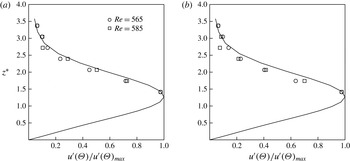
Figure 11. Wall-normal azimuthal velocity fluctuation eigenfunctions at two radii corresponding to $Re=565$ and 585 for frequencies of (a) 400 and (b) 450 Hz for a rotating disk with ${\it\omega}=86.5~\text{s}^{-1}$ and $a=0.2$ . The curve is based on linear stability theory.

3.3 Temporal disturbance development with suction

Following the characterization of the basic flow and natural instability development with suction, experiments were performed to document the space–time evolution of controlled disturbance wavepackets that were introduced into the boundary layer on the disk. The disk conditions were the same as with the previous results, namely ${\it\omega}=86.5~\text{s}^{-1}$ and $a=0.2$ .

Short-duration air-pulse disturbances were introduced at a fixed radius in order to follow the development of wavepackets and discern their amplitude growth in space and time. This utilized the air-pulse disturbance generator developed by Othman & Corke (Reference Othman and Corke2006). The air pulses introduced disturbance wavepackets that featured a broad range of frequencies that could be selectively amplified by the boundary layer. The radial location of the air-pulse generator corresponded to a Reynolds number of $Re=518$ . The hot wire was placed at different Reynolds numbers (radial locations) and azimuthal locations relative to the air-pulser jet. The symbols in figure 12(b) show the relative positions of the air-pulse generator and hot-wire measurement locations. Figure 12(a) is a sketch of the expected wavepacket path spiralling out from the air-pulse generator origin. The relative radial and azimuthal spacings between the disturbance generator and the hot wire were used to document the temporal and spatial growth of the disturbances that were introduced. The documentation of the temporal growth was the key element in confirming the absolute instability.

Figure 12. A schematic of the relative positions between the hot wire and the air-pulse jet with expected wavepacket paths (a) and actual locations of wavepacket ensemble measurements (b).

The air pressure provided to the air-pulse generator was the same 28 p.s.i. as used by Othman & Corke (Reference Othman and Corke2006). Figure 2 documented that this produced a very similar temporal velocity pulse to their previous experiments. In addition, this supply pressure was verified by Othman and Corke to produce wavepackets that exhibited wall-normal azimuthal velocity fluctuation distributions that matched linear theory eigenfunctions.

The sequence for acquiring the velocity time series with the air pulses consisted of acquiring the hot-wire voltage time series for a time duration of four disk revolutions. In a few cases that were mostly at more inboard radial locations, six disk revolutions were acquired. The air pulse was initiated approximately 3 s after the start of data acquisition. Therefore, data were acquired before and after the air pulse. The time in the data series was subsequently referenced to the time at which the air pulse was generated, which was recorded along with the velocity time series. The contiguous time series at a given Re– ${\it\theta}$ location generally consisted of approximately 1000 air-pulse events, corresponding to a total of approximately 4000 disk rotations.

Othman & Corke (Reference Othman and Corke2006) determined the leading and trailing edges of the wavepackets generated by the air pulses by ensemble-averaging the time series using the pulse initiation as a time reference. They subsequently employed a Hilbert transform to determine the envelope of the peak velocity fluctuations within the wavepacket.

A different approach was used in the present work to identify the wavepackets. This involved matched filtering in which the time series following the first disturbance pulse was correlated with the time series that followed from subsequent pulses. Matched filtering is widely used in one-dimensional signal detection applications such as radar and digital communications (Turin Reference Turin1960; Thomas Reference Thomas1965) and in image processing (Andrews Reference Andrews1970). In the present approach, matched filtering provides a measure of the temporal correlation between the time series which can be used to identify the bounds of the wavepackets. The correlations were performed in the frequency domain using a digital FFT. The time series each corresponded to four disk rotations. The matched-filter outputs were averaged over the approximately 1000 air-pulse events. No other filtering of the time series was performed.

Examples of the output from the matched filtering are shown in figure 13. This figure shows disturbance wavepackets obtained by ensemble-averaging the time series in the manner of Othman & Corke (Reference Othman and Corke2006), along with the corresponding averaged matched-filter output. The height of the measurement from the disk surface corresponded to $z^{\ast }=1.414$ , which was the position nearest to the fluctuation amplitude maximum in the azimuthal velocity wall-normal eigenfunction shown in figure 11 that could be reached with the hot wire.

Figure 13. Examples of ensemble-averaged time series and the corresponding matched-filter output based on azimuthal velocity fluctuations measured at (a)  $Re=530$ , ${\it\theta}=10^{\circ }$ and (b)  $Re=560$ , ${\it\theta}=20^{\circ }$ .

The ensemble-averaged time series is made up of higher-frequency fluctuations that are representative of the azimuthal velocity fluctuations associated with the growing and decaying cross-flow modes excited by the air-pulse disturbance. The frequency content of such wavepackets will be presented later in the paper. The matched-filter output corresponds to the smooth curve that envelops the higher-frequency fluctuations. This smooth curve best suits our objective of locating the leading and trailing edges of the wavepackets as they evolve in space and time on the disk.

The evolution of the disturbance wavepackets as indicated by the matched-filter envelopes is shown in figures 14–16. These figures show discrete azimuthal locations relative to the air-pulse generator for $0.89\leqslant Re/Re_{c_{A}}\leqslant 1$ . This range of Reynolds numbers was chosen to present because they encompass where the spreading of the wavepacket departed from that found by Othman & Corke (Reference Othman and Corke2006) with $a=0.$ . At the lower-Reynolds-number locations, the envelope of the wavepacket is evident over an azimuthal extent of $10^{\circ }\leqslant {\it\theta}\leqslant 40^{\circ }$ . As it evolves radially outward to higher Reynolds numbers, the envelope of the wavepacket expands in time (number of disk rotations, $T$ ). In addition, by the last two Reynolds number locations, the azimuthal extent shifts towards larger angles of $20^{\circ }\leqslant {\it\theta}\leqslant 70^{\circ }$ . This angular shift in the envelope of the wavepacket reflects the manner in which the disturbances travel along a log spiral from the disturbance source. We have attempted to represent the development of the wavepacket envelope along the log-spiral trajectory based on the most amplified linear mode in figure 17. Because of their discrete nature, the presented locations do not exactly follow the log spiral. However, it does provide a sense of the motion and spreading of the wavepacket envelope.

Figure 14. Matched-filter output at $Re/Re_{c_{A}}=0.89$ (a,c,e,g,i) and 0.92 (b,d,f,h,j) for ${\it\theta}=10^{\circ }$ (a,b), $20^{\circ }$ (c,d), $30^{\circ }$ (e,f), $40^{\circ }$ (g,h) and $70^{\circ }$ (i,j) locations from the air-pulse generator.

Figure 15. Matched-filter output at $Re/Re_{c_{A}}=0.93$ (a,c,e,g,i) and 0.95 (b,d,f,h,j) for ${\it\theta}=10^{\circ }$ (a,b), $20^{\circ }$ (c,d), $30^{\circ }$ (e,f), $40^{\circ }$ (g,h) and $70^{\circ }$ (i,j) locations from the air-pulse generator.

Figure 16. Matched-filter output at $Re/Re_{c_{A}}=0.99$ (a,c,e,g,i) and 1.00 (b,d,f,h,j) for ${\it\theta}=10^{\circ }$ (a,b), $20^{\circ }$ (c,d), $30^{\circ }$ (e,f), $40^{\circ }$ (g,h) and $70^{\circ }$ (i,j) locations from the air-pulse generator.

Figure 17. Matched-filter output at increasing Reynolds numbers and azimuthal angles which follow the approximate log-spiral path from the air-pulse generator of the most amplified linear cross-flow mode: (a)  $Re=540$ , ${\it\theta}=10$ ; (b) $Re=550$ , ${\it\theta}=20$ ; (c) $Re=560$ , ${\it\theta}=20$ ; (d) $Re=580$ , ${\it\theta}=40$ ; (e) $Re=645$ , ${\it\theta}=70$ .

The wavepacket envelopes such as those shown in figures 14–16 were analysed in order to identify their leading and trailing edges. This was performed in an automated manner in which the output from the matched-filter operation was scanned to determine the maximum and minimum values of the envelope, and the $t/T$ location of the envelope maximum. The leading edge of the envelope was found by searching backwards in time from the location of the envelope maximum to the point at which the value of the envelope was 5 % of the dynamic range (envelope maximum minus envelope minimum). The trailing edge of the envelope was found by searching forward in time from the location of the envelope maximum to the point at which the value of the envelope was again 5 % of the dynamic range. The 5 % threshold was based a determination of what was consistent with a visual inspection of the envelopes. The results were not found to change significantly for thresholds between 4 % and 6 % of the dynamic range. The result of this analysis of the wavepackets is shown in figure 18.

Figure 18. Space–time map of leading-edge (LE) and trailing-edge (TE) locations of disturbance wavepackets for a rotating disk with $86.5~\text{s}^{-1}$ and $a=0.2$ . The solid red curve is the space–time map from Othman & Corke (Reference Othman and Corke2006) with $a=0$ . The upward-arrow data points signify that the trailing-edge location exceeded the four-disk-rotation-time-series limit. The dashed curve is an exponential fit to the TE data from $0.88\leqslant Re/Re_{c_{A}}\leqslant 0.96$ that was extrapolated to $Re_{c_{A}}=1.0$ .

The open and closed symbols in figure 18 correspond to the leading and trailing edges of the wavepackets respectively. The upward-arrow symbols signify data points where the location of the trailing edge was beyond the four-rotation-time-series limit, that is $t/T>4$ . In order to compare with the previous wavepacket measurements of Othman & Corke (Reference Othman and Corke2006), without disk suction, the Reynolds number is normalized by $Re_{c_{A}}$ for two experiments. Without suction, $Re_{c_{A}}=507$ , compared with 650 with $a=0.2$ . Time is normalized by the disk rotation period, $T$ .

The solid red curves in figure 18 correspond to the space–time development of the wavepackets from Othman & Corke (Reference Othman and Corke2006) without disk suction. For the leading edge of the wavepacket, we observe very good agreement in the space–time development between the present experiment and that of Othman & Corke (Reference Othman and Corke2006). For the trailing-edge development, there is good agreement between the two experiments up to $Re/Re_{c_{A}}=0.876$ ( $Re=570$ ). Outboard of that location of the disk, we observe a continual spreading of the wavepacket trailing edge that was not observed by Othman and Corke without suction. The dashed curve is an exponential fit of the trailing-edge data from $0.876\leqslant Re/Re_{c_{A}}\leqslant 0.962$ that was then extrapolated to $Re_{c_{A}}=1.0$ . The three cases denoted by the upward-arrow symbols signify that the trailing-edge locations exceeded the four-disk-rotation limit of the contiguous time series. Unfortunately, the six-rotation-long time series taken at these Reynolds numbers were at azimuthal angles of ${\it\theta}=10^{\circ }$ , where, as indicated in figure 16, the matched filter did not return a coherent wavepacket envelope. This either signifies that the wavepacket was not in that location as it progressed along the log-spiral path, or that the velocity fluctuations were zero, or that they were not correlated with the disturbance pulse. Further analysis will come in examining the velocity fluctuation spectra.

As is evident from the red curve for the wavepacket trailing-edge development without suction (Othman & Corke Reference Othman and Corke2006), the temporal spreading of the wavepackets had asymptoted even as $Re_{c_{A}}$ was approached, which agreed with the simulation observations of Davies & Carpenter (Reference Davies and Carpenter2003). In the present experiment with a wall suction factor of $a=0.2$ , the temporal expansion of the trailing edge of the wavepackets continued to increase exponentially with the Reynolds number, exceeding by approximately a factor of two that without suction at the comparable $Re/Re_{c_{A}}$ . We can only speculate on how far the trailing edge would have continued to expand given that in three cases, and especially at $Re/Re_{c_{A}}\geqslant 0.99$ , the four-rotation-time-series limit was reached. Ideally, in the case of the existence of a global mode, we would expect the trailing-edge spreading to achieve a vertical temporal slope. However, the enhanced spreading of the wavepacket trailing edge in contrast to that without suction documented by Othman & Corke (Reference Othman and Corke2006) suggests support for the predictions of Thomas (Reference Thomas2007) and Thomas & Davies (Reference Thomas and Davies2010).

Another indication of the character of the disturbance wavepackets comes from examining the frequency content of the velocity fluctuations associated with the wavepackets. These were obtained from the same time series on which the matched filtering was performed. Each record of the spectra consisted of the contiguous four-rotation time series. The time series was digitally band-pass filtered in the frequency domain using a specially designed finite impulse response (FIR) filter with a low-pass cutoff of 200 Hz and a high-pass cutoff of 1200 Hz. This was intended to highlight frequencies that are associated with the most amplified linear cross-flow mode, which for our experimental conditions was near 400 Hz, and the most amplified absolute instability mode, which was near 750 Hz. The resulting spectra were averaged over approximately 1000 records, each triggered by the pressure pulse. The amplitude of the spectra corresponds to the r.m.s. of the azimuthal velocity fluctuations with a 1 Hz bandwidth.

Figures 19 and 20 show spectra for the ${\it\theta}=10^{\circ }$ , $20^{\circ }$ , $30^{\circ }$ , $40^{\circ }$ and $70^{\circ }$ locations from the air-pulse generator for a subset of the Reynolds numbers of the wavepacket envelopes that were shown in figures 14–16. Figure 19(a,c,e,g,i) is at the same Reynolds number location ( $Re/Re_{c_{A}}=0.88$ ) as the matched-filter amplitude envelopes in figure 14(a,c,e,g,i). In the latter, the absence of a coherent wavepacket envelope at ${\it\theta}=70^{\circ }$ coincides with very low velocity fluctuations observed in the spectrum at that azimuthal location. Thus, we can surmise that the disturbance wavepacket produced by the pressure pulse had not spread to that azimuthal position.

At $Re/Re_{c_{A}}=0.93$ , the matched-filter amplitude envelopes in figure 15(a,c,e,g,i) still do not reveal a coherent wavepacket. However, the corresponding spectra shown in figure 19(b,d,f,h,j) reveal the influence of the pressure pulse at ${\it\theta}=70^{\circ }$ , with energy appearing in the most amplified linear theory band of frequencies.

The spectra for $Re/Re_{c_{A}}=0.99$ and 1.00 are shown in figure 20. On comparing these with the previous spectra, they immediately reflect the spatial growth in amplitude of the velocity fluctuations associated with the pressure pulse. Another feature is that the amplitude magnitude and frequency distribution is nearly uniform across the azimuthal angle locations. This is revealing because the corresponding wavepacket envelopes that were presented in figure 16 indicated that the velocity fluctuations were not correlated with the disturbance pulse at the ${\it\theta}=10^{\circ }$ location. Since the fluctuation amplitudes are not zero, this might indicate that the boundary layer has undergone turbulent transition.

Figure 19. Spectra of azimuthal velocity fluctuations triggered on pressure pulses at $Re/Re_{c_{A}}=0.89$ (a,c,e,g,i) and 0.93 (b,d,f,h,j) for ${\it\theta}=10^{\circ }$ (a,b), $20^{\circ }$ (c,d), $30^{\circ }$ (e,f), $40^{\circ }$ (g,h) and $70^{\circ }$ (i,j) locations from the air-pulse generator.

Figure 20. Spectra of azimuthal velocity fluctuations triggered on pressure pulses at $Re/Re_{c_{A}}=0.99$ (a,c,e,g,i) and 1.00 (b,d,f,h,j) for ${\it\theta}=10^{\circ }$ (a,b), $20^{\circ }$ (c,d), $30^{\circ }$ (e,f), $40^{\circ }$ (g,h) and $70^{\circ }$ (i,j) locations from the air-pulse generator.

In order to further show the full evolution of the velocity fluctuations that emanate from the disturbance air pulse, spectra like those presented in figures 19 and 20, but at all of the measured radii, were compiled to produce the contour plots shown in figure 21. These plots show the amplitudes in ( $Re,{\it\theta}$ )-space at two frequencies of 450 and 750 Hz, which are representative of the most amplified linear cross-flow mode and the predicted absolute instability mode respectively. The amplitudes have been normalized by their minimum value and presented as log-level contours to highlight exponential growth. The solid curve corresponds to a log spiral with a spiral angle of ${\it\psi}=10.36^{\circ }$ that is based on ${\it\beta}=0.0698$ and the most amplified ${\it\alpha}_{r}=0.382$ for $a=0.2$ . Over the small-azimuthal-angle range, this looks almost linear. The log spiral is drawn to originate from the location of the air-pulse generator, which was at $Re=518$ .

Figure 21. Spatial amplitude distributions produced by the pulse generator shown as contours of $\log (u^{\prime }({\it\theta})/u^{\prime }({\it\theta})_{min})$ for frequencies of 450 Hz (a) and 750 Hz (b). The solid curve corresponds to a log spiral with a spiral angle of ${\it\beta}=0.0698$ that originates from the disturbance source.

Figure 22. The spatial development of the normalized azimuthal velocity fluctuations measured along log spirals in plots in figure 21. The lines correspond to a least-square curve fit of the data to an exponential function.

Close to the air-pulse generator, the disturbance is only felt at small azimuthal angles from the generator. Therefore, the velocity fluctuations at larger angles are much lower, at baseline levels. As illustrated by the previous plots, the disturbance wavepacket forms and expands. This is evident in the contour plots by the rapid azimuthal expansion of velocity fluctuation amplitudes that occurs at approximately $Re=560$ ( $Re/Re_{c_{A}}=0.86$ ). Since this is reflective of the growth of the wavepacket, this occurs for the full spectrum of velocity fluctuations, observed at both 450 and 750 Hz. Outboard of this radius, the amplitudes of the disturbances, reflected in the two selected frequencies, grow steadily. The uniform spacing between contours indicates that the growth is exponential. This continues out to $Re_{c_{A}}=650$ without an indication of saturating.

This is further examined by plotting the growth in the fluctuation amplitudes at the two selected frequencies while following the log-spiral trajectory. The result is shown in figure 22. Here again the amplitude is normalized by the minimum value at each frequency and presented as a log value to highlight exponential growth. The initial azimuthal expansion of the disturbance wavepacket is again evident up to $Re/Re_{c_{A}}=0.86$ . Outboard of that radius, the amplitudes at the two selected frequencies grow exponentially, which is signified by the straight line fits to the data. We note that there is a change in the slope of the linear fits which signifies a change in the growth rate. The change in slope occurs at the same location, $Re/Re_{c_{A}}=0.95$ , for both of the selected frequencies. Prior to that radius, the growth rate at 450 Hz is larger than that at 750 Hz, which is expected based on linear stability theory. However, at $Re/Re_{c_{A}}=0.95$ , the growth rates at both frequencies increase, and appear to be the same. This suggests that the whole spectral band is increasing in amplitude, which one might expect if the boundary layer was transitioning to turbulence. Is there a significance to the $Re/Re_{c_{A}}=0.95$ where this occurs? Based on the space–time evolution of the disturbance wavepacket that was shown in figure 18, this is well within the region of the exponential temporal spreading of the wavepacket trailing edge, and of course close to the expected location of the absolute instability. Although compelling, turbulent transition in itself does not guarantee the presence of a global mode.