


1 Introduction
The direct numerical simulations (DNS) presented in this paper are carried out in order to obtain a detailed understanding of the effect of various levels of contamination on gas transfer across the air–water interface driven by isotropic turbulence diffusing from below. Because of their low mass diffusivity (high Schmidt number) in water, the gas transfer process for low to moderately soluble gases (e.g. oxygen, carbon dioxide, carbon monoxide, methane) is controlled by the hydrodynamics at the liquid side (e.g. Jähne & Haussecker Reference Jähne and Haussecker1998) which significantly depend on the surface condition. In nature, a truly clean surface is almost impossible to maintain. Hence, it is of key importance to understand in detail the effects of surface contamination on the interfacial mass transfer. In the natural environment, several types of surface contamination can be found. In the present paper we assume the surfactant to be insoluble, such as oleyl alcohol. However, the dynamics of low-solubility monolayer-type surfactants with a significantly higher concentration at the surface than in the bulk can be approximately simulated using the aforementioned assumption. Examples of such monolayer films due to organic matter can be found in e.g. Espedal, Johannessen & Knulst (Reference Espedal, Johannessen and Knulst1996). Other types of contamination, such as the presence of a thick layer of crude oil on the water surface, fall outside the scope of this paper. Because of the different mechanisms of scalar transfer, to simulate this type of contamination a two layer structure with different molecular diffusivities needs to be resolved.
Contamination by e.g. surfactants changes the near-surface hydrodynamic conditions by the generation of tangential stresses due to variations in surface elasticity, which under clean conditions is constant. These stresses damp the turbulent eddies near the surface (see Davies Reference Davies1972). For example, Handler et al. (Reference Handler, Leighton, Smith and Nagaosa2003) and Shen, Yue & Triantafyllou (Reference Shen, Yue and Triantafyllou2004) studied the effect of surfactants on free-surface turbulent flow and showed that the surface divergence and associated upwellings and downwellings can be significantly reduced by the presence of even small amounts of surfactants. For large amounts of surfactants Shen et al. (Reference Shen, Yue and Triantafyllou2004) showed that the surface divergence becomes negligibly small and, hence, these up and downwellings almost completely disappear. Consequently, this damping of vertical turbulent motion close to the surface will lead to a decrease in the transfer velocity,
 $K_{L}$
, of atmospheric gases across the air–water interface. For instance, in the experiments of Asher & Pankow (Reference Asher and Pankow1986) and McKenna & McGillis (Reference McKenna and McGillis2004), compared to clean conditions, surface contamination was found to result in a reduction in
$K_{L}$
, of atmospheric gases across the air–water interface. For instance, in the experiments of Asher & Pankow (Reference Asher and Pankow1986) and McKenna & McGillis (Reference McKenna and McGillis2004), compared to clean conditions, surface contamination was found to result in a reduction in
 $K_{L}$
of up to 80 %. This is in agreement with the DNS results of Herlina & Wissink (Reference Herlina and Wissink2016) who studied the limit case of severe contamination (i.e. a no-slip condition) at a Schmidt number of
$K_{L}$
of up to 80 %. This is in agreement with the DNS results of Herlina & Wissink (Reference Herlina and Wissink2016) who studied the limit case of severe contamination (i.e. a no-slip condition) at a Schmidt number of
 $Sc=500$
, which is typical for oxygen. In the hybrid DNS/large-eddy simulation study of Hasegawa & Kasagi (Reference Hasegawa and Kasagi2008) the effect of surface contamination on surface shear driven interfacial mass transfer was studied for
$Sc=500$
, which is typical for oxygen. In the hybrid DNS/large-eddy simulation study of Hasegawa & Kasagi (Reference Hasegawa and Kasagi2008) the effect of surface contamination on surface shear driven interfacial mass transfer was studied for
 $Sc=1$
and 100. For the higher value of
$Sc=1$
and 100. For the higher value of
 $Sc$
a reduction in
$Sc$
a reduction in
 $K_{L}$
of approximately 65 % compared to clean conditions was obtained.
$K_{L}$
of approximately 65 % compared to clean conditions was obtained.
The transfer of atmospheric gases into water is dominated by molecular diffusion resulting in a concentration boundary layer adjacent to the surface. The thickness of this boundary layer (typically
 $10{-}1000~\unicode[STIX]{x03BC}\text{m}$
for
$10{-}1000~\unicode[STIX]{x03BC}\text{m}$
for
 $Sc\approx 500{-}700$
) is usually controlled by turbulence generated by e.g. wind shear, buoyancy or bottom shear. Near the surface this turbulent motion periodically brings up unsaturated fluid from the bulk. During a certain time interval
$Sc\approx 500{-}700$
) is usually controlled by turbulence generated by e.g. wind shear, buoyancy or bottom shear. Near the surface this turbulent motion periodically brings up unsaturated fluid from the bulk. During a certain time interval
 $\unicode[STIX]{x0394}t$
(the renewal time) this fluid is subsequently transported along the surface, where it becomes saturated with atmospheric gases due to diffusion, before it is returned to the bulk. The surface renewal model of Danckwerts (Reference Danckwerts1951) uses an exponential distribution of the renewal time to obtain the relationship
$\unicode[STIX]{x0394}t$
(the renewal time) this fluid is subsequently transported along the surface, where it becomes saturated with atmospheric gases due to diffusion, before it is returned to the bulk. The surface renewal model of Danckwerts (Reference Danckwerts1951) uses an exponential distribution of the renewal time to obtain the relationship
 $K_{L}\sim \sqrt{Dr}$
, where
$K_{L}\sim \sqrt{Dr}$
, where
 $D$
is the diffusion coefficient and
$D$
is the diffusion coefficient and
 $r=1/\unicode[STIX]{x0394}t$
is the surface renewal rate. In this surface renewal model
$r=1/\unicode[STIX]{x0394}t$
is the surface renewal rate. In this surface renewal model
 $r$
implicitly describes the hydrodynamical effects and needs to be determined experimentally. Using DNS results of open-channel flow, Kermani et al. (Reference Kermani, Khakpour, Shen and Igusa2011) showed that Danckwerts’ assumption of a constant surface renewal rate is only approximately valid for larger (older) surface ages.
$r$
implicitly describes the hydrodynamical effects and needs to be determined experimentally. Using DNS results of open-channel flow, Kermani et al. (Reference Kermani, Khakpour, Shen and Igusa2011) showed that Danckwerts’ assumption of a constant surface renewal rate is only approximately valid for larger (older) surface ages.
Fortescue & Pearson (Reference Fortescue and Pearson1967) assumed that the largest eddies in the flow determine the surface renewal rate so that
 $r$
is estimated by
$r$
is estimated by
 $u_{\infty }/\unicode[STIX]{x1D6EC}$
, where
$u_{\infty }/\unicode[STIX]{x1D6EC}$
, where
 $u_{\infty }$
is the root-mean-square (r.m.s.) of the turbulent fluctuations and
$u_{\infty }$
is the root-mean-square (r.m.s.) of the turbulent fluctuations and
 $\unicode[STIX]{x1D6EC}$
is the characteristic length scale of the largest eddies. Hence, the transfer velocity predicted by using this ‘large-eddy model’ is defined by
$\unicode[STIX]{x1D6EC}$
is the characteristic length scale of the largest eddies. Hence, the transfer velocity predicted by using this ‘large-eddy model’ is defined by
 $K_{L}\propto \sqrt{Du_{\infty }/\unicode[STIX]{x1D6EC}}$
. Alternatively, by assuming that small rather than large eddies determine the surface renewal rate, Banerjee, Scott & Rhodes (Reference Banerjee, Scott and Rhodes1968) and Lamont & Scott (Reference Lamont and Scott1970) derived the ‘small-eddy model’, where
$K_{L}\propto \sqrt{Du_{\infty }/\unicode[STIX]{x1D6EC}}$
. Alternatively, by assuming that small rather than large eddies determine the surface renewal rate, Banerjee, Scott & Rhodes (Reference Banerjee, Scott and Rhodes1968) and Lamont & Scott (Reference Lamont and Scott1970) derived the ‘small-eddy model’, where
 $r$
is approximated by
$r$
is approximated by
 $(\unicode[STIX]{x1D716}/\unicode[STIX]{x1D708})^{1/2}$
, in which
$(\unicode[STIX]{x1D716}/\unicode[STIX]{x1D708})^{1/2}$
, in which
 $\unicode[STIX]{x1D716}$
is the turbulent dissipation rate near the surface and
$\unicode[STIX]{x1D716}$
is the turbulent dissipation rate near the surface and
 $\unicode[STIX]{x1D708}$
is the kinematic viscosity. The transfer velocity is subsequently estimated by
$\unicode[STIX]{x1D708}$
is the kinematic viscosity. The transfer velocity is subsequently estimated by
 $K_{L}\propto \sqrt{D(\unicode[STIX]{x1D716}/\unicode[STIX]{x1D708})^{1/2}}$
. By non-dimensionalising the large and small eddy models using
$K_{L}\propto \sqrt{D(\unicode[STIX]{x1D716}/\unicode[STIX]{x1D708})^{1/2}}$
. By non-dimensionalising the large and small eddy models using
 $u_{\infty }$
and
$u_{\infty }$
and
 $\unicode[STIX]{x1D6EC}$
, we obtain
$\unicode[STIX]{x1D6EC}$
, we obtain
 $$\begin{eqnarray}\frac{K_{L}}{u_{\infty }}=c_{1}Sc^{-1/2}R_{T}^{-1/2}\end{eqnarray}$$
and
 $$\begin{eqnarray}\frac{K_{L}}{u_{\infty }}=c_{2}Sc^{-1/2}R_{T}^{-1/4},\end{eqnarray}$$
respectively, where
 $Sc=\unicode[STIX]{x1D708}/D$
,
$Sc=\unicode[STIX]{x1D708}/D$
,
 $R_{T}=u_{\infty }\unicode[STIX]{x1D6EC}/\unicode[STIX]{x1D708}$
is the turbulent Reynolds number and
$R_{T}=u_{\infty }\unicode[STIX]{x1D6EC}/\unicode[STIX]{x1D708}$
is the turbulent Reynolds number and
 $c_{1}$
,
$c_{1}$
,
 $c_{2}$
are constants of proportionality. Note that in (1.2)
$c_{2}$
are constants of proportionality. Note that in (1.2)
 $\unicode[STIX]{x1D716}$
is estimated by
$\unicode[STIX]{x1D716}$
is estimated by
 $\unicode[STIX]{x1D716}=u_{\infty }^{3}/\unicode[STIX]{x1D6EC}$
. In this form, the only difference between the two models lies in the exponent of
$\unicode[STIX]{x1D716}=u_{\infty }^{3}/\unicode[STIX]{x1D6EC}$
. In this form, the only difference between the two models lies in the exponent of
 $R_{T}$
. Theofanous, Houze & Brumfield (Reference Theofanous, Houze and Brumfield1976) recognised the existence of two regimes, where the large- and small-eddy models are valid for low and high
$R_{T}$
. Theofanous, Houze & Brumfield (Reference Theofanous, Houze and Brumfield1976) recognised the existence of two regimes, where the large- and small-eddy models are valid for low and high
 $R_{T}$
, respectively, with a critical turbulent Reynolds number of
$R_{T}$
, respectively, with a critical turbulent Reynolds number of
 $R_{T,crit}\approx 500$
.
$R_{T,crit}\approx 500$
.
An important variant of the surface renewal model is the surface divergence model of McCready, Vassiliadou & Hanratty (Reference McCready, Vassiliadou and Hanratty1986),
 $$\begin{eqnarray}K_{L}=c_{\unicode[STIX]{x1D6FD}}\sqrt{D\unicode[STIX]{x1D6FD}_{rms}},\end{eqnarray}$$
where the r.m.s. of the surface divergence,
 $\unicode[STIX]{x1D6FD}_{rms}$
, is used as a measure for the renewal rate. They showed the importance of surface divergence in interfacial mass transfer. This result was subsequently confirmed in various experimental and numerical studies (e.g. McKenna & McGillis Reference McKenna and McGillis2004; Magnaudet & Calmet Reference Magnaudet and Calmet2006; Kermani et al.
Reference Kermani, Khakpour, Shen and Igusa2011; Herlina & Wissink Reference Herlina and Wissink2014; Turney Reference Turney2016; Wissink & Herlina Reference Wissink and Herlina2016) showing that surface divergence can provide a good quality prediction of the transfer velocity, although the constant of proportionality
$\unicode[STIX]{x1D6FD}_{rms}$
, is used as a measure for the renewal rate. They showed the importance of surface divergence in interfacial mass transfer. This result was subsequently confirmed in various experimental and numerical studies (e.g. McKenna & McGillis Reference McKenna and McGillis2004; Magnaudet & Calmet Reference Magnaudet and Calmet2006; Kermani et al.
Reference Kermani, Khakpour, Shen and Igusa2011; Herlina & Wissink Reference Herlina and Wissink2014; Turney Reference Turney2016; Wissink & Herlina Reference Wissink and Herlina2016) showing that surface divergence can provide a good quality prediction of the transfer velocity, although the constant of proportionality
 $c_{\unicode[STIX]{x1D6FD}}$
was found to vary significantly from case to case. To circumvent uncertainties in the definition of a renewal event, some researchers proposed mixed models of surface renewal and divergence (e.g. Peirson & Banner Reference Peirson and Banner2003).
$c_{\unicode[STIX]{x1D6FD}}$
was found to vary significantly from case to case. To circumvent uncertainties in the definition of a renewal event, some researchers proposed mixed models of surface renewal and divergence (e.g. Peirson & Banner Reference Peirson and Banner2003).
In the numerical investigations of Shen et al. (Reference Shen, Yue and Triantafyllou2004), Hasegawa & Kasagi (Reference Hasegawa and Kasagi2008) and Khakpour, Shen & Yue (Reference Khakpour, Shen and Yue2011) a drastic reduction in
 $\unicode[STIX]{x1D6FD}_{rms}$
was observed with increasing contamination levels. Based on this it was concluded that using a no-slip interfacial boundary condition would be a good approximation of a severely contaminated air–water interface. Based on the findings of Ledwell (Reference Ledwell1984) and Coantic (Reference Coantic1986), it is now generally accepted that for a free-slip surface (clean conditions) the transfer velocity
$\unicode[STIX]{x1D6FD}_{rms}$
was observed with increasing contamination levels. Based on this it was concluded that using a no-slip interfacial boundary condition would be a good approximation of a severely contaminated air–water interface. Based on the findings of Ledwell (Reference Ledwell1984) and Coantic (Reference Coantic1986), it is now generally accepted that for a free-slip surface (clean conditions) the transfer velocity
 $K_{L}$
scales with
$K_{L}$
scales with
 $Sc^{-1/2}$
, while for a no-slip surface (severely contaminated conditions)
$Sc^{-1/2}$
, while for a no-slip surface (severely contaminated conditions)
 $K_{L}$
scales with
$K_{L}$
scales with
 $Sc^{-2/3}$
. This is in agreement with e.g. Hasegawa & Kasagi (Reference Hasegawa and Kasagi2008) who observed that for higher levels of contamination the interfacial mass transfer scaling as a power of the Schmidt number ‘switches’ from
$Sc^{-2/3}$
. This is in agreement with e.g. Hasegawa & Kasagi (Reference Hasegawa and Kasagi2008) who observed that for higher levels of contamination the interfacial mass transfer scaling as a power of the Schmidt number ‘switches’ from
 $Sc^{-0.5}$
to
$Sc^{-0.5}$
to
 $Sc^{-0.7}$
for clean and severely contaminated surfaces, respectively.
$Sc^{-0.7}$
for clean and severely contaminated surfaces, respectively.
For such a no-slip boundary condition Herlina & Wissink (Reference Herlina and Wissink2016) proposed a modified version of the dual-regime model of Theofanous et al. (Reference Theofanous, Houze and Brumfield1976) given by
 $$\begin{eqnarray}\frac{K_{L}}{u_{\infty }}\propto Sc^{-2/3}R_{T}^{-1/2}\quad \text{for }R_{T}<R_{T,crit},\end{eqnarray}$$
and
 $$\begin{eqnarray}\frac{K_{L}}{u_{\infty }}\propto Sc^{-2/3}R_{T}^{-1/4}\quad \text{for }R_{T}>R_{T,crit}.\end{eqnarray}$$
For isotropic turbulence driven mass transfer, the validity of both the large (1.4) and small (1.5) eddy variant for the no-slip boundary condition was subsequently verified by Herlina & Wissink (Reference Herlina and Wissink2016) using DNS data for both low
 $R_{T}$
(up to
$R_{T}$
(up to
 $Sc=500$
) and high
$Sc=500$
) and high
 $R_{T}$
(up to
$R_{T}$
(up to
 $Sc=32$
). For a free-slip boundary condition (clean surface condition), on the other hand, the validity of the scaling of
$Sc=32$
). For a free-slip boundary condition (clean surface condition), on the other hand, the validity of the scaling of
 $K_{L}$
in (1.1) was verified in Herlina & Wissink (Reference Herlina and Wissink2014) for
$K_{L}$
in (1.1) was verified in Herlina & Wissink (Reference Herlina and Wissink2014) for
 $Sc$
up to
$Sc$
up to
 $500$
and turbulent Reynolds numbers up to
$500$
and turbulent Reynolds numbers up to
 $R_{T}\approx 500$
. Also, for buoyancy driven mass transfer Wissink & Herlina (Reference Wissink and Herlina2016) obtained the correct scaling behaviour of
$R_{T}\approx 500$
. Also, for buoyancy driven mass transfer Wissink & Herlina (Reference Wissink and Herlina2016) obtained the correct scaling behaviour of
 $K_{L}$
with
$K_{L}$
with
 $Sc$
for
$Sc$
for
 $R_{T}\leqslant 50$
and
$R_{T}\leqslant 50$
and
 $Sc$
up to
$Sc$
up to
 $500$
.
$500$
.
It remains to be determined what scaling would apply (if any) for small to moderate levels of contamination. To investigate this let us assume that for any surface condition
 $K_{L}$
can be approximated by
$K_{L}$
can be approximated by
 $$\begin{eqnarray}\frac{K_{L}}{u_{\infty }}=cSc^{-q}R_{T}^{-r},\end{eqnarray}$$
where
 $r=1/2$
and
$r=1/2$
and
 $1/4$
for the low and high
$1/4$
for the low and high
 $R_{T}$
regimes, respectively. In this expression the power
$R_{T}$
regimes, respectively. In this expression the power
 $q$
is related to the level of contamination at the surface. Note that for other flow regimes the scalings in (1.1), (1.2), (1.4) and (1.5) might not be valid, as evidenced by the large spread of parameters obtained in previous works (e.g. Notter & Sleicher Reference Notter and Sleicher1971; Jähne & Haussecker Reference Jähne and Haussecker1998; Na & Hanratty Reference Na and Hanratty2000). Therefore, we decided to avoid any bias due to mean shear and use isotropic turbulence when studying the effect of various levels of surface contamination on interfacial gas transfer.
$q$
is related to the level of contamination at the surface. Note that for other flow regimes the scalings in (1.1), (1.2), (1.4) and (1.5) might not be valid, as evidenced by the large spread of parameters obtained in previous works (e.g. Notter & Sleicher Reference Notter and Sleicher1971; Jähne & Haussecker Reference Jähne and Haussecker1998; Na & Hanratty Reference Na and Hanratty2000). Therefore, we decided to avoid any bias due to mean shear and use isotropic turbulence when studying the effect of various levels of surface contamination on interfacial gas transfer.
As in our previous DNS calculations, surface waves are assumed to be very shallow so that the interface can be modelled using a rigid lid assumption. The contamination level is characterised by
 $Ma/Ca_{T}$
, where
$Ma/Ca_{T}$
, where
 $Ma$
is the Marangoni number and
$Ma$
is the Marangoni number and
 $Ca_{T}$
is the turbulent capillary number (details in § 2.3). In the results presented below, it will be shown that for small levels of contamination, parts of the surface area become virtually surfactant free. A model is subsequently proposed and verified that predicts
$Ca_{T}$
is the turbulent capillary number (details in § 2.3). In the results presented below, it will be shown that for small levels of contamination, parts of the surface area become virtually surfactant free. A model is subsequently proposed and verified that predicts
 $K_{L}$
using the surfactant-free fraction of the surface area.
$K_{L}$
using the surfactant-free fraction of the surface area.
2 Numerical aspects
2.1 Governing equations
The problem that is simulated concerns the reduction in interfacial gas transfer due to surface contaminations in a turbulent water environment driven by isotropic turbulence diffusing from below. The dimensionless incompressible Navier–Stokes equations are defined by the continuity equation
 $$\begin{eqnarray}\frac{\unicode[STIX]{x2202}u_{i}}{\unicode[STIX]{x2202}x_{i}}=0,\end{eqnarray}$$
and the momentum equations
 $$\begin{eqnarray}\frac{\unicode[STIX]{x2202}u_{i}}{\unicode[STIX]{x2202}t}+\frac{\unicode[STIX]{x2202}u_{i}u_{j}}{\unicode[STIX]{x2202}x_{j}}=-\frac{\unicode[STIX]{x2202}p}{\unicode[STIX]{x2202}x_{i}}+\frac{1}{Re}\frac{\unicode[STIX]{x2202}^{2}u_{i}}{\unicode[STIX]{x2202}x_{j}\unicode[STIX]{x2202}x_{j}}\quad (i=1,2,3),\end{eqnarray}$$
where
 $x_{1}=x$
,
$x_{1}=x$
,
 $x_{2}=y$
are the horizontal (surface-parallel) directions and
$x_{2}=y$
are the horizontal (surface-parallel) directions and
 $x_{3}=z$
is the vertical (surface-normal) direction,
$x_{3}=z$
is the vertical (surface-normal) direction,
 $u_{1}=u$
,
$u_{1}=u$
,
 $u_{2}=v$
and
$u_{2}=v$
and
 $u_{3}=w$
are the velocities in the
$u_{3}=w$
are the velocities in the
 $x$
,
$x$
,
 $y$
and
$y$
and
 $z$
directions, respectively,
$z$
directions, respectively,
 $p$
is the pressure,
$p$
is the pressure,
 $Re$
is the Reynolds number and
$Re$
is the Reynolds number and
 $t$
denotes time.
$t$
denotes time.
The dimensionless scalar concentration
 $c^{\ast }$
is governed by the following advection diffusion equation
$c^{\ast }$
is governed by the following advection diffusion equation
 $$\begin{eqnarray}\frac{\unicode[STIX]{x2202}c^{\ast }}{\unicode[STIX]{x2202}t}+\frac{\unicode[STIX]{x2202}u_{j}c^{\ast }}{\unicode[STIX]{x2202}x_{j}}=\frac{1}{Re\,Sc}\frac{\unicode[STIX]{x2202}^{2}c^{\ast }}{\unicode[STIX]{x2202}x_{j}\unicode[STIX]{x2202}x_{j}}\quad (j=1,2,3),\end{eqnarray}$$
where
 $$\begin{eqnarray}c^{\ast }=\frac{c-c_{b,0}}{c_{s}-c_{b,0}},\end{eqnarray}$$
in which
 $c_{b,0}$
is the initial concentration in the bulk and
$c_{b,0}$
is the initial concentration in the bulk and
 $c_{s}$
is the concentration at the surface, which is assumed to be fully saturated at all times. At the bottom of the domain a Neumann boundary condition of zero scalar flux (
$c_{s}$
is the concentration at the surface, which is assumed to be fully saturated at all times. At the bottom of the domain a Neumann boundary condition of zero scalar flux (
 $\unicode[STIX]{x2202}c/\unicode[STIX]{x2202}z=0$
) is imposed.
$\unicode[STIX]{x2202}c/\unicode[STIX]{x2202}z=0$
) is imposed.
At the surface the following two-dimensional transport equation for the surfactant concentration is solved
 $$\begin{eqnarray}\frac{\unicode[STIX]{x2202}\unicode[STIX]{x1D6FE}^{\ast }}{\unicode[STIX]{x2202}t}+\frac{\unicode[STIX]{x2202}u_{j}\unicode[STIX]{x1D6FE}^{\ast }}{\unicode[STIX]{x2202}x_{j}}=\frac{1}{Re\,Sc_{s}}\frac{\unicode[STIX]{x2202}^{2}\unicode[STIX]{x1D6FE}^{\ast }}{\unicode[STIX]{x2202}x_{j}\unicode[STIX]{x2202}x_{j}}\quad (j=1,2),\end{eqnarray}$$
where
 $\unicode[STIX]{x1D6FE}^{\ast }$
is defined as the surfactant concentration,
$\unicode[STIX]{x1D6FE}^{\ast }$
is defined as the surfactant concentration,
 $\unicode[STIX]{x1D6FE}$
, non-dimensionalised by the equilibrium concentration
$\unicode[STIX]{x1D6FE}$
, non-dimensionalised by the equilibrium concentration
 $\unicode[STIX]{x1D6FE}_{0}$
. Note that a rigid lid assumption was employed and the surfactant concentration at the surface was assumed to be conserved at all times. The latter implies that the surfactant is insoluble, whereby absorption and desorption processes as well as chemical kinetics that may affect the surfactant concentration are ignored. An example of such a surfactant often used in experiments is oleyl alcohol (e.g. McKenna & McGillis Reference McKenna and McGillis2004; Salter et al.
Reference Salter, Upstill-Goddard, Nightingale, Archer, Blomquist, Ho, Huebert, Schlosser and Yang2011). Typical concentrations of this surfactant that would correspond to the levels of contamination investigated in this paper range from 0 to approximately
$\unicode[STIX]{x1D6FE}_{0}$
. Note that a rigid lid assumption was employed and the surfactant concentration at the surface was assumed to be conserved at all times. The latter implies that the surfactant is insoluble, whereby absorption and desorption processes as well as chemical kinetics that may affect the surfactant concentration are ignored. An example of such a surfactant often used in experiments is oleyl alcohol (e.g. McKenna & McGillis Reference McKenna and McGillis2004; Salter et al.
Reference Salter, Upstill-Goddard, Nightingale, Archer, Blomquist, Ho, Huebert, Schlosser and Yang2011). Typical concentrations of this surfactant that would correspond to the levels of contamination investigated in this paper range from 0 to approximately
 $0.1~\unicode[STIX]{x03BC}\text{g}~\text{cm}^{-2}$
.
$0.1~\unicode[STIX]{x03BC}\text{g}~\text{cm}^{-2}$
.
Similar to
 $\unicode[STIX]{x1D6FE}^{\ast }$
, the surface tension
$\unicode[STIX]{x1D6FE}^{\ast }$
, the surface tension
 $\unicode[STIX]{x1D70E}$
is also made dimensionless using its equilibrium value
$\unicode[STIX]{x1D70E}$
is also made dimensionless using its equilibrium value
 $\unicode[STIX]{x1D70E}_{0}$
. At the water surface
$\unicode[STIX]{x1D70E}_{0}$
. At the water surface
 $\unicode[STIX]{x1D70E}^{\ast }=\unicode[STIX]{x1D70E}/\unicode[STIX]{x1D70E}_{0}$
is assumed to linearly depend on
$\unicode[STIX]{x1D70E}^{\ast }=\unicode[STIX]{x1D70E}/\unicode[STIX]{x1D70E}_{0}$
is assumed to linearly depend on
 $\unicode[STIX]{x1D6FE}^{\ast }$
– which is a significant idealisation of the real-world behaviour of surfactants – so that the Marangoni number, defined by
$\unicode[STIX]{x1D6FE}^{\ast }$
– which is a significant idealisation of the real-world behaviour of surfactants – so that the Marangoni number, defined by
 $$\begin{eqnarray}Ma=\left.-\frac{\text{d}\unicode[STIX]{x1D70E}^{\ast }}{\text{d}\unicode[STIX]{x1D6FE}^{\ast }}\right|_{\unicode[STIX]{x1D6FE}^{\ast }=1},\end{eqnarray}$$
is constant. Note that it is assumed that the surface tension only depends on the surfactant concentration, other factors (such as temperature variations and interfacial viscosity) are assumed to be negligible. Also, in the remainder of this paper
 $c$
and
$c$
and
 $\unicode[STIX]{x1D6FE}$
rather than
$\unicode[STIX]{x1D6FE}$
rather than
 $c^{\ast }$
and
$c^{\ast }$
and
 $\unicode[STIX]{x1D6FE}^{\ast }$
, respectively, will be used to refer to the non-dimensional concentrations.
$\unicode[STIX]{x1D6FE}^{\ast }$
, respectively, will be used to refer to the non-dimensional concentrations.
Based on the model presented in Shen et al. (Reference Shen, Yue and Triantafyllou2004) the effect of the surface contamination on the near surface velocity fluctuations is modelled by relating the normal gradient of the horizontal velocities at the surface (
 $z=L_{z}$
) to the horizontal gradients of the surfactant concentration
$z=L_{z}$
) to the horizontal gradients of the surfactant concentration
 $$\begin{eqnarray}\displaystyle & \displaystyle \left.\frac{\unicode[STIX]{x2202}u}{\unicode[STIX]{x2202}z}\right|_{z=L_{z}}=-\frac{Ma}{Ca}\frac{\unicode[STIX]{x2202}\unicode[STIX]{x1D6FE}}{\unicode[STIX]{x2202}x} & \displaystyle\end{eqnarray}$$
 $$\begin{eqnarray}\displaystyle & \displaystyle \left.\frac{\unicode[STIX]{x2202}v}{\unicode[STIX]{x2202}z}\right|_{z=L_{z}}=-\frac{Ma}{Ca}\frac{\unicode[STIX]{x2202}\unicode[STIX]{x1D6FE}}{\unicode[STIX]{x2202}y}, & \displaystyle\end{eqnarray}$$
where
 $Ca=\unicode[STIX]{x1D707}U/\unicode[STIX]{x1D70E}$
is the capillary number and
$Ca=\unicode[STIX]{x1D707}U/\unicode[STIX]{x1D70E}$
is the capillary number and
 $\unicode[STIX]{x1D707}$
is the dynamic viscosity. In the presence of mean shear, the parameter
$\unicode[STIX]{x1D707}$
is the dynamic viscosity. In the presence of mean shear, the parameter
 $Ma/Ca$
is typically presented using the equivalent expression
$Ma/Ca$
is typically presented using the equivalent expression
 $Re\,Ma/We$
, where
$Re\,Ma/We$
, where
 $We$
is the Weber number. Because in our case the mean shear is zero, we prefer to use the capillary number. Note that when slight vertical deformations of the interface are simulated, a more sophisticated model is required (e.g. Tsai Reference Tsai1996).
$We$
is the Weber number. Because in our case the mean shear is zero, we prefer to use the capillary number. Note that when slight vertical deformations of the interface are simulated, a more sophisticated model is required (e.g. Tsai Reference Tsai1996).
2.2 Numerical method
The incompressible Navier–Stokes equations were discretised using fourth-order accurate central discretisations of advection and diffusion (see Wissink Reference Wissink2004) combined with the second-order Adams–Bashforth method for the time integration. The scalar transport equations (2.3) and (2.5) were solved using the fifth-order accurate weighted essentially non-oscillatory (WENO) scheme of Liu, Osher & Chan (Reference Liu, Osher and Chan1994) for the convective terms combined with a fourth-order accurate central discretisation for the diffusion. For the time integration of the scalar equations a three-stage Runge–Kutta method was used. To deal with low scalar diffusivities some of the scalars were solved on a finer mesh than the flow field (cf. § 2.3). Parallelisation was achieved by dividing the computational domain into blocks of equal size. Each block was assigned to its own processing core in order to obtain a near-optimal load balancing. The standard message passing interface (MPI) protocol was employed for communication between blocks. See Kubrak et al. (Reference Kubrak, Herlina, Greve and Wissink2013) and Herlina & Wissink (Reference Herlina and Wissink2014) for a more detailed description of the numerical method.
2.3 Overview of simulations
As in our previous simulations (Herlina & Wissink Reference Herlina and Wissink2014, Reference Herlina and Wissink2016) the choice of the computational domain was based on the experiments performed by Herlina & Jirka (Reference Herlina and Jirka2008) where turbulence was induced by an oscillating grid near the bottom of a water tank (cf. figure 1). In the present direct numerical simulations a computational domain of size
 $L_{x}\times L_{y}\times L_{z}=5L\times 5L\times 3L$
is employed, where the reference length scale
$L_{x}\times L_{y}\times L_{z}=5L\times 5L\times 3L$
is employed, where the reference length scale
 $L$
is chosen arbitrarily to be 1 cm. In all simulations, a Reynolds number of
$L$
is chosen arbitrarily to be 1 cm. In all simulations, a Reynolds number of
 $Re=UL/\unicode[STIX]{x1D708}=600$
is selected, where – for a kinematic viscosity of
$Re=UL/\unicode[STIX]{x1D708}=600$
is selected, where – for a kinematic viscosity of
 $\unicode[STIX]{x1D708}=10^{-2}$
cm
$\unicode[STIX]{x1D708}=10^{-2}$
cm
 $^{2}$
s
$^{2}$
s
 $^{-1}$
– the reference velocity is
$^{-1}$
– the reference velocity is
 $U=6$
cm s
$U=6$
cm s
 $^{-1}$
. Note that not
$^{-1}$
. Note that not
 $Re$
but a turbulent Reynolds number
$Re$
but a turbulent Reynolds number
 $R_{T}$
– which is determined from the results – will be used to present and analyse the data below. Also, in the remainder of this paper – unless stated otherwise – all velocity, time and length scales have been non-dimensionalised using
$R_{T}$
– which is determined from the results – will be used to present and analyse the data below. Also, in the remainder of this paper – unless stated otherwise – all velocity, time and length scales have been non-dimensionalised using
 $U$
and
$U$
and
 $L$
. The flow is resolved using a
$L$
. The flow is resolved using a
 $128\times 128\times 212$
base mesh that is stretched in the
$128\times 128\times 212$
base mesh that is stretched in the
 $z$
-direction to concentrate grid points near the interface (i.e. near
$z$
-direction to concentrate grid points near the interface (i.e. near
 $z=L_{z}$
). The mass transfer calculation is performed for
$z=L_{z}$
). The mass transfer calculation is performed for
 $Sc=2$
, 4, 8, 16, 32. The first two scalars are resolved using the base mesh, while the latter three scalars are solved on a finer mesh with refinement factor 2. Exactly the same mesh was employed in our previous simulation GS200 in Herlina & Wissink (Reference Herlina and Wissink2014), where an extensive grid refinement study was carried out to show the adequacy of the chosen resolution for both flow and scalar fields. Note that in the following analysis
$Sc=2$
, 4, 8, 16, 32. The first two scalars are resolved using the base mesh, while the latter three scalars are solved on a finer mesh with refinement factor 2. Exactly the same mesh was employed in our previous simulation GS200 in Herlina & Wissink (Reference Herlina and Wissink2014), where an extensive grid refinement study was carried out to show the adequacy of the chosen resolution for both flow and scalar fields. Note that in the following analysis
 $\unicode[STIX]{x1D701}=L_{z}-z$
will be additionally used to denote the distance from the free surface. To account for the much larger size of the experimental water tank, periodic boundary conditions are employed in the horizontal directions.
$\unicode[STIX]{x1D701}=L_{z}-z$
will be additionally used to denote the distance from the free surface. To account for the much larger size of the experimental water tank, periodic boundary conditions are employed in the horizontal directions.

Figure 1. Schematic of the computational configuration (a). The configuration was selected in accordance with the grid-stirred turbulence driven gas transfer experiments (b) of Herlina & Jirka (Reference Herlina and Jirka2008), where only a small part adjacent to the surface is modelled.
The input turbulence at
 $z=0$
of the computational domain originated from a concurrently running large-eddy simulation (LES) of fully developed isotropic turbulence. A
$z=0$
of the computational domain originated from a concurrently running large-eddy simulation (LES) of fully developed isotropic turbulence. A
 $64^{3}$
mesh is used to discretize the
$64^{3}$
mesh is used to discretize the
 $(L_{x})^{3}$
periodic box. Note that in Herlina & Wissink (Reference Herlina and Wissink2014), for a similar simulation, it was shown that the missing small scales in the energy spectrum of the LES quickly re-establish and a complete spectrum was obtained within a distance of one-
$(L_{x})^{3}$
periodic box. Note that in Herlina & Wissink (Reference Herlina and Wissink2014), for a similar simulation, it was shown that the missing small scales in the energy spectrum of the LES quickly re-establish and a complete spectrum was obtained within a distance of one-
 $L$
from the bottom of the DNS which is well below the surface influenced layer. The turbulent flow field introduced into the DNS domain is the same in all simulations. The turbulence level is set to
$L$
from the bottom of the DNS which is well below the surface influenced layer. The turbulent flow field introduced into the DNS domain is the same in all simulations. The turbulence level is set to
 $\sqrt{2\langle k\rangle /3}=0.4$
, where
$\sqrt{2\langle k\rangle /3}=0.4$
, where
 $k=\overline{u_{i}^{\prime }u_{i}^{\prime }}/2$
is the turbulent kinetic energy, the prime denotes the fluctuating velocity, while
$k=\overline{u_{i}^{\prime }u_{i}^{\prime }}/2$
is the turbulent kinetic energy, the prime denotes the fluctuating velocity, while
 $\langle \cdot \rangle$
and
$\langle \cdot \rangle$
and
 $\overline{\cdot }$
correspond to averaging in the homogeneous directions and time, respectively. Note that in our DNS
$\overline{\cdot }$
correspond to averaging in the homogeneous directions and time, respectively. Note that in our DNS
 $u_{i}^{\prime }=u_{i}$
.
$u_{i}^{\prime }=u_{i}$
.
Table 1. Overview of the simulations.

In total seven simulations with varying
 $Ma/Ca$
numbers ranging from 0 (free slip) to 30 as well as a no-slip case are performed (cf. table 1). Note that although in a hydrodynamics sense the contaminated surface will not converge to a no-slip surface, the scaling of mass transfer with
$Ma/Ca$
numbers ranging from 0 (free slip) to 30 as well as a no-slip case are performed (cf. table 1). Note that although in a hydrodynamics sense the contaminated surface will not converge to a no-slip surface, the scaling of mass transfer with
 $Sc$
for the no-slip case agrees well with the scaling found for severely contaminated surface conditions where
$Sc$
for the no-slip case agrees well with the scaling found for severely contaminated surface conditions where
 $Ma/Ca$
approaches
$Ma/Ca$
approaches
 $\infty$
(see § 4.2). The boundary condition at the top depends on
$\infty$
(see § 4.2). The boundary condition at the top depends on
 $Ma/Ca$
and affects the near-surface turbulence, resulting in variations in the turbulent fluctuations
$Ma/Ca$
and affects the near-surface turbulence, resulting in variations in the turbulent fluctuations
 $$\begin{eqnarray}u_{rms}(\unicode[STIX]{x1D701})=\sqrt{\overline{\langle u^{\prime }u^{\prime }\rangle }}\end{eqnarray}$$
and the longitudinal integral length scale
 $$\begin{eqnarray}L_{11}(\unicode[STIX]{x1D701})=\int _{0}^{L_{x}/2}R_{11}(r,\unicode[STIX]{x1D701})\,\text{d}r,\end{eqnarray}$$
where the longitudinal two-point correlation
 $R_{11}$
of the horizontal velocity is defined by
$R_{11}$
of the horizontal velocity is defined by
 $$\begin{eqnarray}R_{11}(r,\unicode[STIX]{x1D701})=\frac{\displaystyle \int _{x=0}^{L_{x}/2}\int _{y=0}^{L_{y}}u^{\prime }(x,y,\unicode[STIX]{x1D701})u^{\prime }(x+r,y,\unicode[STIX]{x1D701})\,\text{d}y\,\text{d}x}{\displaystyle \int _{x=0}^{L_{x}/2}\int _{y=0}^{L_{y}}u^{\prime 2}(x,y,\unicode[STIX]{x1D701})\,\text{d}y\,\text{d}x},\end{eqnarray}$$
where
 $L_{x}\times L_{y}$
is the size of the horizontal plane. To allow a direct comparison between the different simulations, the characteristic turbulent velocity and length scales are all evaluated at the same location
$L_{x}\times L_{y}$
is the size of the horizontal plane. To allow a direct comparison between the different simulations, the characteristic turbulent velocity and length scales are all evaluated at the same location
 $\unicode[STIX]{x1D701}=L$
, which approximately corresponds to a distance equal to
$\unicode[STIX]{x1D701}=L$
, which approximately corresponds to a distance equal to
 $L_{\infty }$
from the surface (cf. table 1), so that
$L_{\infty }$
from the surface (cf. table 1), so that
 $$\begin{eqnarray}u_{\infty }=u_{rms}|_{\unicode[STIX]{x1D701}=L}\end{eqnarray}$$
and
 $$\begin{eqnarray}L_{\infty }=\overline{L_{11}}|_{\unicode[STIX]{x1D701}=L}.\end{eqnarray}$$
The appropriateness of the location where
 $u_{\infty }$
and
$u_{\infty }$
and
 $L_{\infty }$
are evaluated is further explained in § 4.1. Following the convention typically used for grid-stirred turbulence (e.g. Hopfinger & Toly Reference Hopfinger and Toly1976; Brumley & Jirka Reference Brumley and Jirka1987), we use
$L_{\infty }$
are evaluated is further explained in § 4.1. Following the convention typically used for grid-stirred turbulence (e.g. Hopfinger & Toly Reference Hopfinger and Toly1976; Brumley & Jirka Reference Brumley and Jirka1987), we use
 $\unicode[STIX]{x1D6EC}=2L_{\infty }$
as the characteristic turbulent length scale. Using these scales, the turbulent Reynolds number reads
$\unicode[STIX]{x1D6EC}=2L_{\infty }$
as the characteristic turbulent length scale. Using these scales, the turbulent Reynolds number reads
 $$\begin{eqnarray}R_{T}=\frac{u_{\infty }2L_{\infty }}{\unicode[STIX]{x1D708}}\end{eqnarray}$$
and the turbulent capillary number is given by
 $$\begin{eqnarray}Ca_{T}=\frac{\unicode[STIX]{x1D707}u_{\infty }}{\unicode[STIX]{x1D70E}}.\end{eqnarray}$$
Note that the latter does not depend on the integral length scale. In the following analysis, the level of surface contamination will be characterised by the parameter
 $Ma/Ca_{T}$
and time averaging is performed from
$Ma/Ca_{T}$
and time averaging is performed from
 $t=150$
to
$t=150$
to
 $t=300$
, corresponding to approximately seven eddy turnover times (
$t=300$
, corresponding to approximately seven eddy turnover times (
 $2L_{\infty }/u_{\infty }$
).
$2L_{\infty }/u_{\infty }$
).
Khakpour et al. (Reference Khakpour, Shen and Yue2011) showed that the actual Schmidt number of the surfactant is not important for an accurate calculation of the surfactant concentration. Hence, it is decided to perform all simulations using a surfactant Schmidt number of
 $Sc_{s}=2$
.
$Sc_{s}=2$
.
3 Proposed estimation of mean
 $K_{L}$
based on clean surface fraction
$\overline{\unicode[STIX]{x1D6FC}}$
$K_{L}$
based on clean surface fraction
$\overline{\unicode[STIX]{x1D6FC}}$


As mentioned above, it is likely that the exponent
 $q$
in (1.6) will depend on the level of surface contamination. Based on this idea, we propose an estimation for both
$q$
in (1.6) will depend on the level of surface contamination. Based on this idea, we propose an estimation for both
 $q$
and
$q$
and
 $c$
by using the average clean surface fraction
$c$
by using the average clean surface fraction
 $\overline{\unicode[STIX]{x1D6FC}}$
(suitably defined by means of a threshold, cf. § 4.2.4), which is likely to be a relatively ‘easy observable’ parameter. Our proposed model for
$\overline{\unicode[STIX]{x1D6FC}}$
(suitably defined by means of a threshold, cf. § 4.2.4), which is likely to be a relatively ‘easy observable’ parameter. Our proposed model for
 $cSc^{-q}$
in (1.6) reads
$cSc^{-q}$
in (1.6) reads
 $$\begin{eqnarray}cSc^{-q}=\overline{\unicode[STIX]{x1D6FC}}c_{f}Sc^{-q_{f}}+(1-\overline{\unicode[STIX]{x1D6FC}})c_{n}Sc^{-q_{n}},\end{eqnarray}$$
with
 $q_{f}\leqslant q\leqslant q_{n}$
, where
$q_{f}\leqslant q\leqslant q_{n}$
, where
 $q_{f},c_{f}$
and
$q_{f},c_{f}$
and
 $q_{n},c_{n}$
correspond to the exponents of
$q_{n},c_{n}$
correspond to the exponents of
 $Sc$
and the constants of proportionality for the free-slip and no-slip cases, respectively. To obtain expressions for
$Sc$
and the constants of proportionality for the free-slip and no-slip cases, respectively. To obtain expressions for
 $c$
and
$c$
and
 $q$
based on
$q$
based on
 $\overline{\unicode[STIX]{x1D6FC}}$
we substitute the following Taylor expansions
$\overline{\unicode[STIX]{x1D6FC}}$
we substitute the following Taylor expansions
 $$\begin{eqnarray}\displaystyle & Sc^{-q_{f}}=Sc^{-(q-h_{1})}\approx Sc^{-q}+h_{1}(\ln Sc)Sc^{-q}+O(h_{1}^{2}) & \displaystyle\end{eqnarray}$$
 $$\begin{eqnarray}\displaystyle & Sc^{-q_{n}}=Sc^{-(q+h_{2})}\approx Sc^{-q}-h_{2}(\ln Sc)Sc^{-q}+O(h_{2}^{2}) & \displaystyle\end{eqnarray}$$
into (3.1) and after ignoring the second- and higher-order terms, we obtain:
 $$\begin{eqnarray}cSc^{-q}=[\overline{\unicode[STIX]{x1D6FC}}c_{f}(1+h_{1}\ln Sc)+(1-\overline{\unicode[STIX]{x1D6FC}})c_{n}(1-h_{2}\ln Sc)]Sc^{-q}.\end{eqnarray}$$
Assuming
 $c$
is independent of
$c$
is independent of
 $Sc$
, it is necessary to eliminate
$Sc$
, it is necessary to eliminate
 $\ln Sc$
from this expression, which is achieved when
$\ln Sc$
from this expression, which is achieved when
 $$\begin{eqnarray}\overline{\unicode[STIX]{x1D6FC}}c_{f}h_{1}-(1-\overline{\unicode[STIX]{x1D6FC}})c_{n}h_{2}=0.\end{eqnarray}$$
If we replace
 $h_{1}$
by
$h_{1}$
by
 $\unicode[STIX]{x1D6E5}_{nf}-h_{2}$
, where
$\unicode[STIX]{x1D6E5}_{nf}-h_{2}$
, where
 $\unicode[STIX]{x1D6E5}_{nf}=q_{n}-q_{f}$
we obtain
$\unicode[STIX]{x1D6E5}_{nf}=q_{n}-q_{f}$
we obtain
 $$\begin{eqnarray}\displaystyle & \displaystyle h_{2}=\frac{\unicode[STIX]{x1D6E5}_{nf}\overline{\unicode[STIX]{x1D6FC}}c_{f}}{(1-\overline{\unicode[STIX]{x1D6FC}})c_{n}+\overline{\unicode[STIX]{x1D6FC}}c_{f}} & \displaystyle\end{eqnarray}$$
 $$\begin{eqnarray}\displaystyle & q=q_{n}-h_{2} & \displaystyle\end{eqnarray}$$
 $$\begin{eqnarray}\displaystyle & c=\overline{\unicode[STIX]{x1D6FC}}c_{f}+(1-\overline{\unicode[STIX]{x1D6FC}})c_{n}. & \displaystyle\end{eqnarray}$$
In accordance to the literature, the exponents
 $q_{f}$
and
$q_{f}$
and
 $q_{n}$
are fixed to
$q_{n}$
are fixed to
 $1/2$
and
$1/2$
and
 $2/3$
, respectively. The parameters
$2/3$
, respectively. The parameters
 $c_{f}$
and
$c_{f}$
and
 $c_{n}$
will be determined from results of the free-slip and no-slip cases. Subsequently,
$c_{n}$
will be determined from results of the free-slip and no-slip cases. Subsequently,
 $K_{L}/(u_{\infty }R_{T}^{-r})$
can be predicted as a function of
$K_{L}/(u_{\infty }R_{T}^{-r})$
can be predicted as a function of
 $\overline{\unicode[STIX]{x1D6FC}}$
alone using (3.6), (3.8) and (1.6). The quality of the proposed prediction will be investigated in § 4.4.
$\overline{\unicode[STIX]{x1D6FC}}$
alone using (3.6), (3.8) and (1.6). The quality of the proposed prediction will be investigated in § 4.4.
4 Results
4.1 Turbulent flow statistics
Before discussing the effect of surface contamination levels on interfacial mass transfer, we will briefly discuss its influence on turbulent flow statistics. As mentioned in § 2.3, in all seven simulations the same turbulent flow field is introduced at
 $z=0$
, whilst at the surface (
$z=0$
, whilst at the surface (
 $z=L_{z}$
) different levels of contamination are imposed by varying
$z=L_{z}$
) different levels of contamination are imposed by varying
 $Ma/Ca_{T}$
. Figure 2(a,b) illustrates the decay of the turbulence as it diffuses upwards. For all simulations, the levels of horizontal (surface-parallel) and vertical (surface-normal) fluctuations in the lower part of the computational domain (up to
$Ma/Ca_{T}$
. Figure 2(a,b) illustrates the decay of the turbulence as it diffuses upwards. For all simulations, the levels of horizontal (surface-parallel) and vertical (surface-normal) fluctuations in the lower part of the computational domain (up to
 $z\approx 1.5L$
) were found to be almost identical, while up to
$z\approx 1.5L$
) were found to be almost identical, while up to
 $z=2L$
the flow was still found to be largely isotropic. Closer to the surface (i.e. in the surface influenced layer) differences become noticeable. Responsible for this are the different boundary conditions at the surface, where the vertical velocity is always zero, while the horizontal velocities depend on
$z=2L$
the flow was still found to be largely isotropic. Closer to the surface (i.e. in the surface influenced layer) differences become noticeable. Responsible for this are the different boundary conditions at the surface, where the vertical velocity is always zero, while the horizontal velocities depend on
 $Ma/Ca_{T}$
. As a consequence, the variation in the level of vertical fluctuations is much smaller than in the horizontal fluctuations. In agreement with previous numerical results (e.g. Perot & Moin Reference Perot and Moin1995; Walker, Leighton & Garza-Rios Reference Walker, Leighton and Garza-Rios1996; Calmet & Magnaudet Reference Calmet and Magnaudet2003), for the free-slip case (S0)
$Ma/Ca_{T}$
. As a consequence, the variation in the level of vertical fluctuations is much smaller than in the horizontal fluctuations. In agreement with previous numerical results (e.g. Perot & Moin Reference Perot and Moin1995; Walker, Leighton & Garza-Rios Reference Walker, Leighton and Garza-Rios1996; Calmet & Magnaudet Reference Calmet and Magnaudet2003), for the free-slip case (S0)
 $w_{rms}$
is found to suddenly decrease towards the surface while
$w_{rms}$
is found to suddenly decrease towards the surface while
 $u_{rms}$
simultaneously increases (a more detailed discussion can be found in Herlina & Wissink Reference Herlina and Wissink2014).
$u_{rms}$
simultaneously increases (a more detailed discussion can be found in Herlina & Wissink Reference Herlina and Wissink2014).

Figure 2. Effect of
 $Ma/Ca_{T}$
on the near-surface turbulent flow statistics: (a)
$Ma/Ca_{T}$
on the near-surface turbulent flow statistics: (a)
 $u_{rms}$
, (b)
$u_{rms}$
, (b)
 $w_{rms}$
. (c,d) the same as (a,b) plotted in logarithmic scale and using the inverse coordinate
$w_{rms}$
. (c,d) the same as (a,b) plotted in logarithmic scale and using the inverse coordinate
 $\unicode[STIX]{x1D701}=L_{z}-z$
. Shown are time-averaged (
$\unicode[STIX]{x1D701}=L_{z}-z$
. Shown are time-averaged (
 $t=150{-}300$
) results.
$t=150{-}300$
) results.
Figure 2(c) shows a more detailed view of the
 $u_{rms}$
profiles near the surface. With the exception of the no-slip simulation (SN), the horizontal fluctuation levels were observed to coincide reasonably well up to
$u_{rms}$
profiles near the surface. With the exception of the no-slip simulation (SN), the horizontal fluctuation levels were observed to coincide reasonably well up to
 $z\approx 2.8L$
(or
$z\approx 2.8L$
(or
 $\unicode[STIX]{x1D701}\approx 0.2L$
). The different result obtained for SN is due to the application of a no-slip boundary condition at the surface, while in the other simulations the surface velocity field is merely forced to become more and more divergence free with increasing
$\unicode[STIX]{x1D701}\approx 0.2L$
). The different result obtained for SN is due to the application of a no-slip boundary condition at the surface, while in the other simulations the surface velocity field is merely forced to become more and more divergence free with increasing
 $Ma/Ca_{T}$
. From
$Ma/Ca_{T}$
. From
 $z\approx 2.8L$
to the surface the horizontal fluctuations in S0 and S1 were found to increase, while in all other simulations
$z\approx 2.8L$
to the surface the horizontal fluctuations in S0 and S1 were found to increase, while in all other simulations
 $u_{rms}$
decreases. In general, it is observed that
$u_{rms}$
decreases. In general, it is observed that
 $u_{rms}$
in S0–S5 tends to slightly decrease with increasing
$u_{rms}$
in S0–S5 tends to slightly decrease with increasing
 $Ma/Ca_{T}$
, whereby the results from S0 and S1 as well as S4 and S5 almost coincide. This decrease in
$Ma/Ca_{T}$
, whereby the results from S0 and S1 as well as S4 and S5 almost coincide. This decrease in
 $u_{rms}$
illustrates that rising levels of surface contamination tend to increase near-surface turbulence damping. The increase in
$u_{rms}$
illustrates that rising levels of surface contamination tend to increase near-surface turbulence damping. The increase in
 $u_{rms}$
observed in S0 and S1 is caused by the redistribution of turbulent kinetic energy: close to the surface the vertical velocity fluctuations decline and as a result the horizontal fluctuations are enlarged (see also Perot & Moin Reference Perot and Moin1995). The aforementioned rising levels of surface contamination result in increased instantaneous shear and, hence, in increased damping of
$u_{rms}$
observed in S0 and S1 is caused by the redistribution of turbulent kinetic energy: close to the surface the vertical velocity fluctuations decline and as a result the horizontal fluctuations are enlarged (see also Perot & Moin Reference Perot and Moin1995). The aforementioned rising levels of surface contamination result in increased instantaneous shear and, hence, in increased damping of
 $u_{rms}$
as can be seen in figure 2(c) for S2–S5.
$u_{rms}$
as can be seen in figure 2(c) for S2–S5.
Figure 2(d) shows that the
 $w_{rms}$
profiles exhibit a similar decreasing trend with
$w_{rms}$
profiles exhibit a similar decreasing trend with
 $Ma/Ca_{T}$
as observed for
$Ma/Ca_{T}$
as observed for
 $u_{rms}$
above. This decrease in
$u_{rms}$
above. This decrease in
 $w_{rms}$
is expected to affect the interfacial mass transfer, which is further investigated in § 4.2.2 below. Note that the
$w_{rms}$
is expected to affect the interfacial mass transfer, which is further investigated in § 4.2.2 below. Note that the
 $w_{rms}$
profiles from both S0 and S1 as well as S5 and SN almost coincide. It can be easily seen from Taylor series expansions that close to the surface
$w_{rms}$
profiles from both S0 and S1 as well as S5 and SN almost coincide. It can be easily seen from Taylor series expansions that close to the surface
 $w_{rms}$
is proportional to
$w_{rms}$
is proportional to
 $\unicode[STIX]{x1D701}^{2}$
in the no-slip case, while in the free-slip case
$\unicode[STIX]{x1D701}^{2}$
in the no-slip case, while in the free-slip case
 $w_{rms}\propto \unicode[STIX]{x1D701}$
. Both trends are consistently reproduced by our simulations SN and S0, respectively. The near surface
$w_{rms}\propto \unicode[STIX]{x1D701}$
. Both trends are consistently reproduced by our simulations SN and S0, respectively. The near surface
 $w_{rms}$
in simulations S1 to S4 (
$w_{rms}$
in simulations S1 to S4 (
 $0<Ma/Ca_{T}\leqslant 54$
) is found to behave similarly to the free-slip simulation with
$0<Ma/Ca_{T}\leqslant 54$
) is found to behave similarly to the free-slip simulation with
 $w_{rms}\propto \unicode[STIX]{x1D701}$
. Only in S5 where
$w_{rms}\propto \unicode[STIX]{x1D701}$
. Only in S5 where
 $Ma/Ca_{T}=269$
an intermediate behaviour between free slip and no slip is found with
$Ma/Ca_{T}=269$
an intermediate behaviour between free slip and no slip is found with
 $w_{rms}\propto \unicode[STIX]{x1D701}^{1.36}$
.
$w_{rms}\propto \unicode[STIX]{x1D701}^{1.36}$
.
With the exception of the no-slip simulation SN, all cases have a non-zero two-dimensional (2-D) velocity field at the surface. While in the free-slip simulation the velocity field quickly becomes three-dimensional with increasing depth (as
 $w\propto \unicode[STIX]{x1D701}$
), in cases with large
$w\propto \unicode[STIX]{x1D701}$
), in cases with large
 $Ma/Ca_{T}$
this takes much longer as
$Ma/Ca_{T}$
this takes much longer as
 $w\propto \unicode[STIX]{x1D701}^{2}$
. The latter is a result of the Marangoni effect – caused by horizontal gradients in the surfactant concentration – inducing a force counteracting the aforementioned surfactant gradients thereby effectively forcing the 2-D flow at the surface to become almost divergence free (
$w\propto \unicode[STIX]{x1D701}^{2}$
. The latter is a result of the Marangoni effect – caused by horizontal gradients in the surfactant concentration – inducing a force counteracting the aforementioned surfactant gradients thereby effectively forcing the 2-D flow at the surface to become almost divergence free (
 $\unicode[STIX]{x2202}u/\unicode[STIX]{x2202}x+\unicode[STIX]{x2202}v/\unicode[STIX]{x2202}y\approx 0$
).
$\unicode[STIX]{x2202}u/\unicode[STIX]{x2202}x+\unicode[STIX]{x2202}v/\unicode[STIX]{x2202}y\approx 0$
).
For all simulations, the turbulent integral length scale
 $L_{11}$
shown in figure 3(a) is first found to increase with distance from the turbulent source until a local maximum is reached at
$L_{11}$
shown in figure 3(a) is first found to increase with distance from the turbulent source until a local maximum is reached at
 $\unicode[STIX]{x1D701}\approx 0.5L$
. Above this location
$\unicode[STIX]{x1D701}\approx 0.5L$
. Above this location
 $L_{11}$
reduces to zero at the surface in the no-slip case, while in the free-slip simulation and in the low
$L_{11}$
reduces to zero at the surface in the no-slip case, while in the free-slip simulation and in the low
 $Ma/Ca_{T}$
case (S1) it reduces to approximately 0.87 and 0.8, respectively. In S2 to S5 (moderate to large
$Ma/Ca_{T}$
case (S1) it reduces to approximately 0.87 and 0.8, respectively. In S2 to S5 (moderate to large
 $Ma/Ca_{T}$
) the integral length scale is found to increase again when approaching the surface. An explanation of this behaviour is given in the discussion of figure 4 below. It is attributed to the presence of instantaneous shear which becomes stronger with increasing
$Ma/Ca_{T}$
) the integral length scale is found to increase again when approaching the surface. An explanation of this behaviour is given in the discussion of figure 4 below. It is attributed to the presence of instantaneous shear which becomes stronger with increasing
 $Ma/Ca_{T}$
such that for S2 to S5 an increased horizontal integral length scale is obtained.
$Ma/Ca_{T}$
such that for S2 to S5 an increased horizontal integral length scale is obtained.

Figure 3. Vertical variation of (a) turbulent integral length scale
 $L_{11}$
(time averaged from
$L_{11}$
(time averaged from
 $t=150{-}300$
) and (b) Kolmogorov length scale
$t=150{-}300$
) and (b) Kolmogorov length scale
 $\unicode[STIX]{x1D702}$
at
$\unicode[STIX]{x1D702}$
at
 $t=300$
.
$t=300$
.
Figure 3(b) shows the variation of the Kolmogorov scale
 $\unicode[STIX]{x1D702}=(\unicode[STIX]{x1D708}^{3}/\unicode[STIX]{x1D716})^{1/4}$
with distance from the surface for
$\unicode[STIX]{x1D702}=(\unicode[STIX]{x1D708}^{3}/\unicode[STIX]{x1D716})^{1/4}$
with distance from the surface for
 $t=300$
. Note that
$t=300$
. Note that
 $\unicode[STIX]{x1D716}$
is calculated by
$\unicode[STIX]{x1D716}$
is calculated by
 $$\begin{eqnarray}\unicode[STIX]{x1D716}=\langle 2\unicode[STIX]{x1D708}s_{ij}s_{ij}\rangle ,\end{eqnarray}$$
where
 $s_{ij}=(\unicode[STIX]{x2202}u_{i}^{\prime }/\unicode[STIX]{x2202}x_{j}+\unicode[STIX]{x2202}u_{j}^{\prime }/\unicode[STIX]{x2202}x_{i})/2$
. Apart from S0, it can be seen that
$s_{ij}=(\unicode[STIX]{x2202}u_{i}^{\prime }/\unicode[STIX]{x2202}x_{j}+\unicode[STIX]{x2202}u_{j}^{\prime }/\unicode[STIX]{x2202}x_{i})/2$
. Apart from S0, it can be seen that
 $\unicode[STIX]{x1D702}$
increases monotonically from the lower bulk upwards until it reaches a maximum at
$\unicode[STIX]{x1D702}$
increases monotonically from the lower bulk upwards until it reaches a maximum at
 $\unicode[STIX]{x1D701}$
between
$\unicode[STIX]{x1D701}$
between
 $0.1L$
and
$0.1L$
and
 $0.2L$
. For
$0.2L$
. For
 $\unicode[STIX]{x1D701}$
approaching zero two trends can be observed: (i) in S0
$\unicode[STIX]{x1D701}$
approaching zero two trends can be observed: (i) in S0
 $\unicode[STIX]{x1D702}$
becomes constant and (ii) in all other cases
$\unicode[STIX]{x1D702}$
becomes constant and (ii) in all other cases
 $\unicode[STIX]{x1D702}$
decreases, indicating vortex stretching which is most likely caused by instantaneous shear forces. In SN this shear is caused by the no-slip boundary condition, while in S1–S5 it is induced by the Marangoni forces.
$\unicode[STIX]{x1D702}$
decreases, indicating vortex stretching which is most likely caused by instantaneous shear forces. In SN this shear is caused by the no-slip boundary condition, while in S1–S5 it is induced by the Marangoni forces.

Figure 4. Vortical structures identified using the isosurface of
 $\unicode[STIX]{x1D706}_{2}=-0.001$
from simulations (a) S0, (b) S4, (c) S5. The isosurfaces are coloured by the distance
$\unicode[STIX]{x1D706}_{2}=-0.001$
from simulations (a) S0, (b) S4, (c) S5. The isosurfaces are coloured by the distance
 $\unicode[STIX]{x1D701}$
from the surface.
$\unicode[STIX]{x1D701}$
from the surface.
Using representative snapshots the effect of shearing on the interfacial integral length scale
 $L_{11}$
is illustrated by visualising the vortical structures close to the surface (cf. figure 4) using the
$L_{11}$
is illustrated by visualising the vortical structures close to the surface (cf. figure 4) using the
 $\unicode[STIX]{x1D706}_{2}$
criterion of Jeong & Hussain (Reference Jeong and Hussain1995). Compared to S4 and S5, in S0 significantly fewer vortical structures managed to reach the surface whereby the axes of these structures were found to be orthogonal to the surface. In S4 and S5 both the diameter and the orientation of a significant proportion of the vortex tubes that reach the surface differ from the ones observed in S0. In S0 the vortex tubes have a constant diameter and are orientated perpendicular to the surface. The former is in agreement with the constant
$\unicode[STIX]{x1D706}_{2}$
criterion of Jeong & Hussain (Reference Jeong and Hussain1995). Compared to S4 and S5, in S0 significantly fewer vortical structures managed to reach the surface whereby the axes of these structures were found to be orthogonal to the surface. In S4 and S5 both the diameter and the orientation of a significant proportion of the vortex tubes that reach the surface differ from the ones observed in S0. In S0 the vortex tubes have a constant diameter and are orientated perpendicular to the surface. The former is in agreement with the constant
 $\unicode[STIX]{x1D702}$
between
$\unicode[STIX]{x1D702}$
between
 $\unicode[STIX]{x1D701}=0.1$
and 0 as observed in figure 3(b). Contrary, in S4 and S5 many vortex tubes are non-orthogonal to the surface such that their horizontal cross-sectional area widens towards the surface, which may contribute to a larger
$\unicode[STIX]{x1D701}=0.1$
and 0 as observed in figure 3(b). Contrary, in S4 and S5 many vortex tubes are non-orthogonal to the surface such that their horizontal cross-sectional area widens towards the surface, which may contribute to a larger
 $L_{11}$
at the surface. This non-orthogonality can be explained by the instantaneous shear induced by the Marangoni forces at the surface. Note that the apparent widening of the horizontal cross-sectional area of vortex tubes towards the interface in S4 and S5 does not imply that the actual diameter of the vortex tubes increases. Instead, the diameter of the tubes is known to scale with the Kolmogorov length scale which was observed to decrease towards the surface as shown in figure 3(b). In contrast to the no-slip simulation SN – where it is impossible for vortices to reach the surface as the velocity field is zero – the vortex structures in S4 and S5 do reach the surface indicating that the case
$L_{11}$
at the surface. This non-orthogonality can be explained by the instantaneous shear induced by the Marangoni forces at the surface. Note that the apparent widening of the horizontal cross-sectional area of vortex tubes towards the interface in S4 and S5 does not imply that the actual diameter of the vortex tubes increases. Instead, the diameter of the tubes is known to scale with the Kolmogorov length scale which was observed to decrease towards the surface as shown in figure 3(b). In contrast to the no-slip simulation SN – where it is impossible for vortices to reach the surface as the velocity field is zero – the vortex structures in S4 and S5 do reach the surface indicating that the case
 $Ma/Ca_{T}\rightarrow \infty$
is hydrodynamically different from the no-slip case.
$Ma/Ca_{T}\rightarrow \infty$
is hydrodynamically different from the no-slip case.
Figure 5 shows the turbulent Reynolds number profiles of S0, S2, S4, SN. In agreement with earlier studies of grid-stirred generated turbulence diffusing upwards, eventually the horizontal turbulent fluctuations
 $u_{rms}$
are observed to scale with
$u_{rms}$
are observed to scale with
 $z^{-1}$
, while the integral length scale
$z^{-1}$
, while the integral length scale
 $L_{11}$
increases with
$L_{11}$
increases with
 $z$
(e.g. Brumley & Jirka Reference Brumley and Jirka1987). Consequently, their product – and hence
$z$
(e.g. Brumley & Jirka Reference Brumley and Jirka1987). Consequently, their product – and hence
 $R_{T}$
– becomes constant, which in our simulations is achieved between
$R_{T}$
– becomes constant, which in our simulations is achieved between
 $z=1.5L$
and
$z=1.5L$
and
 $2.25L$
, illustrating the appropriateness of our choice to evaluate
$2.25L$
, illustrating the appropriateness of our choice to evaluate
 $L_{\infty }$
and
$L_{\infty }$
and
 $u_{\infty }$
at
$u_{\infty }$
at
 $z=2L$
. Note that this location corresponds to the edge of the surface influenced layer (cf. figure 2).
$z=2L$
. Note that this location corresponds to the edge of the surface influenced layer (cf. figure 2).

Figure 5. Effect of
 $Ma/Ca_{T}$
on
$Ma/Ca_{T}$
on
 $R_{T}$
. Shown are time-averaged (
$R_{T}$
. Shown are time-averaged (
 $t=150{-}300$
) results.
$t=150{-}300$
) results.
4.2 Influence of
$Ma/Ca_{T}$

4.2.1 Qualitative observations
In figure 6 the instantaneous concentration isosurfaces for
 $c_{Sc=4}=0.5$
from simulations S1, S2 and S4 are shown. The isosurfaces are coloured by the corresponding surfactant concentration at the surface
$c_{Sc=4}=0.5$
from simulations S1, S2 and S4 are shown. The isosurfaces are coloured by the corresponding surfactant concentration at the surface
 $\unicode[STIX]{x1D6FE}(x,y)$
which is normalised using the maximum instantaneous concentration
$\unicode[STIX]{x1D6FE}(x,y)$
which is normalised using the maximum instantaneous concentration
 $\unicode[STIX]{x1D6FE}_{max}$
(see also (4.6) below). The plots illustrate the dynamic variation in concentration boundary layer thickness induced by the turbulence from below as discussed previously for clean surfaces by e.g. Nagaosa & Handler (Reference Nagaosa and Handler2003), Magnaudet & Calmet (Reference Magnaudet and Calmet2006) and for clean and severely contaminated surfaces by e.g. Khakpour et al. (Reference Khakpour, Shen and Yue2011). Generally, at the locations where the boundary layer is thin, surfactants are pushed to the side by strong upwelling motions (splats) and subsequently accumulate in the downwelling (antisplats) regions identified by boundary layer thickening. In agreement with the enhanced turbulence damping for increased levels of contamination observed in figure 2, the downwelling is observed to be strongest in S1 as can be seen by the deep penetration of the antisplats into the bulk. Furthermore, in this low
$\unicode[STIX]{x1D6FE}_{max}$
(see also (4.6) below). The plots illustrate the dynamic variation in concentration boundary layer thickness induced by the turbulence from below as discussed previously for clean surfaces by e.g. Nagaosa & Handler (Reference Nagaosa and Handler2003), Magnaudet & Calmet (Reference Magnaudet and Calmet2006) and for clean and severely contaminated surfaces by e.g. Khakpour et al. (Reference Khakpour, Shen and Yue2011). Generally, at the locations where the boundary layer is thin, surfactants are pushed to the side by strong upwelling motions (splats) and subsequently accumulate in the downwelling (antisplats) regions identified by boundary layer thickening. In agreement with the enhanced turbulence damping for increased levels of contamination observed in figure 2, the downwelling is observed to be strongest in S1 as can be seen by the deep penetration of the antisplats into the bulk. Furthermore, in this low
 $Ma/Ca_{T}$
simulation strong upwelling motions result in a large virtually surfactant-free surface fraction (figure 6
a). For increasing
$Ma/Ca_{T}$
simulation strong upwelling motions result in a large virtually surfactant-free surface fraction (figure 6
a). For increasing
 $Ma/Ca_{T}$
this surface fraction becomes rapidly smaller and is found to completely disappear in S4. The connection between
$Ma/Ca_{T}$
this surface fraction becomes rapidly smaller and is found to completely disappear in S4. The connection between
 $Ma/Ca_{T}$
and the surfactant-free area will be further investigated below (cf. § 4.2.4).
$Ma/Ca_{T}$
and the surfactant-free area will be further investigated below (cf. § 4.2.4).

Figure 6. Instantaneous isosurfaces of concentration at
 $c_{Sc=4}=0.5$
from (a) S1, (b) S2 and (c) S4 at
$c_{Sc=4}=0.5$
from (a) S1, (b) S2 and (c) S4 at
 $t=300~L/U$
. The colours represent the normalised surfactant concentration at the corresponding interfacial (
$t=300~L/U$
. The colours represent the normalised surfactant concentration at the corresponding interfacial (
 $x$
,
$x$
,
 $y$
) coordinates.
$y$
) coordinates.
Figure 7 contrasts the correlation between the instantaneous concentration (colour contours) and the surface divergence
 $\unicode[STIX]{x1D6FD}$
(isolines), defined by
$\unicode[STIX]{x1D6FD}$
(isolines), defined by
 $$\begin{eqnarray}\unicode[STIX]{x1D6FD}=\left.\left(\frac{\unicode[STIX]{x2202}u}{\unicode[STIX]{x2202}x}+\frac{\unicode[STIX]{x2202}v}{\unicode[STIX]{x2202}y}\right)\right|_{z=L_{z}},\end{eqnarray}$$
in the grid plane adjacent to the surface in simulations S1 and S5. In S1 areas of low concentration are observed to coincide with strong positive surface divergence indicating upwelling, while in areas of high concentration the surface divergence is found to be negative. In S5, on the other hand, the above correlation becomes less clear and areas with strong positive surface divergence are found not to always coincide with low concentration levels and vice versa. In general, when upwelling first occurs the correlation between low concentration and strong positive surface divergence is found to be very good. At large
 $Ma/Ca_{T}$
(e.g. S5), surface divergence tends to induce strong Marangoni forces that in turn act to reduce surface divergence. As a result, in time the correlation between low concentration regions and strong positive surface divergence is largely lost and instantaneous shear is generated near the surface, as also observed in figure 4 (see also Handler et al.
Reference Handler, Leighton, Smith and Nagaosa2003; Khakpour et al.
Reference Khakpour, Shen and Yue2011). Note that in this respect the high
$Ma/Ca_{T}$
(e.g. S5), surface divergence tends to induce strong Marangoni forces that in turn act to reduce surface divergence. As a result, in time the correlation between low concentration regions and strong positive surface divergence is largely lost and instantaneous shear is generated near the surface, as also observed in figure 4 (see also Handler et al.
Reference Handler, Leighton, Smith and Nagaosa2003; Khakpour et al.
Reference Khakpour, Shen and Yue2011). Note that in this respect the high
 $Ma/Ca_{T}$
simulations S4 and S5 behave like the no-slip case SN.
$Ma/Ca_{T}$
simulations S4 and S5 behave like the no-slip case SN.

Figure 7. Effect of increasing
 $Ma/Ca_{T}$
on the correlation between the dissolved gas concentration (colour contours) and surface divergence (isolines). The solid and dotted lines correspond to positive and negative surface divergence, respectively. Snapshots are from (a) S1 and (b) S5.
$Ma/Ca_{T}$
on the correlation between the dissolved gas concentration (colour contours) and surface divergence (isolines). The solid and dotted lines correspond to positive and negative surface divergence, respectively. Snapshots are from (a) S1 and (b) S5.
4.2.2 Vertical mass flux
Figure 8 shows the effect of
 $Ma/Ca_{T}$
on the mean vertical concentration, the r.m.s. of the concentration fluctuations, and the diffusive and turbulent mass flux profiles from simulations S0, S1, S2, S3 and SN. Note that the profiles from simulations S4 and S5 (not shown here) were found to be almost identical with the SN profiles. Figure 8(a) depicts the normalised mean concentration profiles
$Ma/Ca_{T}$
on the mean vertical concentration, the r.m.s. of the concentration fluctuations, and the diffusive and turbulent mass flux profiles from simulations S0, S1, S2, S3 and SN. Note that the profiles from simulations S4 and S5 (not shown here) were found to be almost identical with the SN profiles. Figure 8(a) depicts the normalised mean concentration profiles
 $$\begin{eqnarray}\frac{\overline{\langle c\rangle }-\overline{\langle c_{b}\rangle }}{c_{s}-\overline{\langle c_{b}\rangle }},\end{eqnarray}$$
where
 $c_{b}$
is evaluated in the bulk at
$c_{b}$
is evaluated in the bulk at
 $z=z_{b}$
, chosen such that
$z=z_{b}$
, chosen such that
 $$\begin{eqnarray}c_{rms}(z_{b})=0.5\max (c_{rms}).\end{eqnarray}$$
It can be seen that an increase in the contamination level leads to a thickening of the mean concentration boundary layer. The thickness
 $\unicode[STIX]{x1D6FF}$
of this layer can be identified by the depth where
$\unicode[STIX]{x1D6FF}$
of this layer can be identified by the depth where
 $c_{rms}$
reaches its maximum. In agreement with the above observation, in figure 8(b) the peak in
$c_{rms}$
reaches its maximum. In agreement with the above observation, in figure 8(b) the peak in
 $c_{rms}$
is seen to move farther from the surface with increasing
$c_{rms}$
is seen to move farther from the surface with increasing
 $Ma/Ca_{T}$
. This thickness
$Ma/Ca_{T}$
. This thickness
 $\unicode[STIX]{x1D6FF}$
was found to gradually increase from 0.0239, 0.0273, 0.0345, 0.0424, 0.0487 for S0, S1, S2, S3, and SN, respectively. Also, with the exception of S0, the peaks in
$\unicode[STIX]{x1D6FF}$
was found to gradually increase from 0.0239, 0.0273, 0.0345, 0.0424, 0.0487 for S0, S1, S2, S3, and SN, respectively. Also, with the exception of S0, the peaks in
 $c_{rms}$
are found to decrease with increasing surface contamination level. The relatively large peak observed in S1 compared to S0 is associated with the stronger up and downwellings caused by an increase in the surface divergence fluctuations (
$c_{rms}$
are found to decrease with increasing surface contamination level. The relatively large peak observed in S1 compared to S0 is associated with the stronger up and downwellings caused by an increase in the surface divergence fluctuations (
 $\unicode[STIX]{x1D6FD}_{rms}$
) in S1 which is explained in more detail in § 4.2.3, cf. discussion of figure 8(b).
$\unicode[STIX]{x1D6FD}_{rms}$
) in S1 which is explained in more detail in § 4.2.3, cf. discussion of figure 8(b).

Figure 8. Effect of
 $Ma/Ca_{T}$
on the horizontally and time-averaged profiles of (a) normalised concentration, (b) normalised concentration fluctuations, (c) vertical scalar diffusion, (d) vertical turbulent scalar flux. In (c,d) the depth
$Ma/Ca_{T}$
on the horizontally and time-averaged profiles of (a) normalised concentration, (b) normalised concentration fluctuations, (c) vertical scalar diffusion, (d) vertical turbulent scalar flux. In (c,d) the depth
 $\unicode[STIX]{x1D701}$
is normalised using the boundary layer thickness. Note that the molecular diffusion coefficient
$\unicode[STIX]{x1D701}$
is normalised using the boundary layer thickness. Note that the molecular diffusion coefficient
 $D$
is defined by
$D$
is defined by
 $D=1/Re\,Sc$
.
$D=1/Re\,Sc$
.
The total vertical mass flux is determined by the sum of the vertical diffusive
 $\overline{\langle -D\unicode[STIX]{x2202}c/\unicode[STIX]{x2202}z\rangle }$
and turbulent
$\overline{\langle -D\unicode[STIX]{x2202}c/\unicode[STIX]{x2202}z\rangle }$
and turbulent
 $\overline{\langle c^{\prime }w^{\prime }\rangle }$
mass fluxes. At the surface the mass flux is entirely due to diffusion. Above it was observed that the boundary layer thickness decreases with decreasing
$\overline{\langle c^{\prime }w^{\prime }\rangle }$
mass fluxes. At the surface the mass flux is entirely due to diffusion. Above it was observed that the boundary layer thickness decreases with decreasing
 $Ma/Ca_{T}$
, as a result the gradients
$Ma/Ca_{T}$
, as a result the gradients
 $\overline{\unicode[STIX]{x2202}c/\unicode[STIX]{x2202}z}$
become steeper leading to an increase of the interfacial mass flux (figure 8
c). Note that for the present no-slip simulation with
$\overline{\unicode[STIX]{x2202}c/\unicode[STIX]{x2202}z}$
become steeper leading to an increase of the interfacial mass flux (figure 8
c). Note that for the present no-slip simulation with
 $R_{T}=117$
this gradient remains constant up to
$R_{T}=117$
this gradient remains constant up to
 $\unicode[STIX]{x1D701}/\unicode[STIX]{x1D6FF}\approx 0.2$
. As a consequence, diffusion fully dominates mass flux not only at the surface but also immediately beneath. This is in agreement with figure 8(d) where the normal gradient of the scalar flux
$\unicode[STIX]{x1D701}/\unicode[STIX]{x1D6FF}\approx 0.2$
. As a consequence, diffusion fully dominates mass flux not only at the surface but also immediately beneath. This is in agreement with figure 8(d) where the normal gradient of the scalar flux
 $\overline{\langle c^{\prime }w^{\prime }\rangle }$
vanishes at the surface. The latter immediately follows from the fact that at the surface (i)
$\overline{\langle c^{\prime }w^{\prime }\rangle }$
vanishes at the surface. The latter immediately follows from the fact that at the surface (i)
 $w^{\prime }=0$
and (ii) the conservation of mass requirement for the no-slip simulation implies that
$w^{\prime }=0$
and (ii) the conservation of mass requirement for the no-slip simulation implies that
 $\unicode[STIX]{x2202}w^{\prime }/\unicode[STIX]{x2202}z=0$
. For larger
$\unicode[STIX]{x2202}w^{\prime }/\unicode[STIX]{x2202}z=0$
. For larger
 $R_{T}$
the distance from the surface for which the above applies reduces, as can be seen in Herlina & Wissink (Reference Herlina and Wissink2016, figure 11(c)), where for
$R_{T}$
the distance from the surface for which the above applies reduces, as can be seen in Herlina & Wissink (Reference Herlina and Wissink2016, figure 11(c)), where for
 $R_{T}=865$
the gradient is only approximately constant up to
$R_{T}=865$
the gradient is only approximately constant up to
 $\unicode[STIX]{x1D701}/\unicode[STIX]{x1D6FF}\approx 0.08$
.
$\unicode[STIX]{x1D701}/\unicode[STIX]{x1D6FF}\approx 0.08$
.
Figure 8(c,d) also show that with increasing distance from the surface the diffusive mass flux rapidly reduces, while simultaneously the turbulent mass flux increases so that the total vertical mass flux is kept constant. Already at a depth of three times the boundary layer thickness the turbulent mass flux almost completely dominates the total mass flux. In agreement with the reduction in the diffusive mass flux at the surface, figure 8(d) shows that the turbulent mass flux in the bulk also reduces with increasing level of contamination.
Figure 9 illustrates the influence of the surface contamination level on the mean transfer velocity
 $K_{L}=\overline{k_{L}}$
, where the instantaneous
$K_{L}=\overline{k_{L}}$
, where the instantaneous
 $k_{L}$
is defined by
$k_{L}$
is defined by
 $$\begin{eqnarray}k_{L}(t)=\frac{\left\langle -D\left.{\displaystyle \frac{\unicode[STIX]{x2202}c}{\unicode[STIX]{x2202}z}}\right|_{z=L_{z}}\right\rangle }{c_{s}-\langle c_{b}\rangle },\end{eqnarray}$$
with
 $D=1/Re\,Sc$
. It can be seen that the average transfer velocity
$D=1/Re\,Sc$
. It can be seen that the average transfer velocity
 $K_{L}$
reduces drastically within a narrow range of
$K_{L}$
reduces drastically within a narrow range of
 $Ma/Ca_{T}=0{-}11$
. For
$Ma/Ca_{T}=0{-}11$
. For
 $Ma/Ca_{T}\geqslant 54$
the time-averaged transfer velocity is found to be similar to the no-slip case. Note that because the resulting
$Ma/Ca_{T}\geqslant 54$
the time-averaged transfer velocity is found to be similar to the no-slip case. Note that because the resulting
 $R_{T}$
in the simulations varies between 114 and 141 – which is well within the region where the large-eddy model is valid (Theofanous et al.
Reference Theofanous, Houze and Brumfield1976; Herlina & Wissink Reference Herlina and Wissink2016) –
$R_{T}$
in the simulations varies between 114 and 141 – which is well within the region where the large-eddy model is valid (Theofanous et al.
Reference Theofanous, Houze and Brumfield1976; Herlina & Wissink Reference Herlina and Wissink2016) –
 $K_{L}$
is normalised by
$K_{L}$
is normalised by
 $R_{T}^{-1/2}$
in order to allow for a direct comparison of the results, as discussed in the Introduction.
$R_{T}^{-1/2}$
in order to allow for a direct comparison of the results, as discussed in the Introduction.

Figure 9. Variation of
 $K_{L}$
with
$K_{L}$
with
 $Ma/Ca_{T}$
for
$Ma/Ca_{T}$
for
 $Sc=32$
.
$Sc=32$
.
In figure 10 the variation of
 $K_{L}$
with Schmidt number is shown. It can be seen that for each individual
$K_{L}$
with Schmidt number is shown. It can be seen that for each individual
 $Ma/Ca_{T}$
case there is a power law dependency
$Ma/Ca_{T}$
case there is a power law dependency
 $K_{L}\propto Sc^{-q}$
. When
$K_{L}\propto Sc^{-q}$
. When
 $Ma/Ca_{T}$
increases from 0 to 54, the exponent
$Ma/Ca_{T}$
increases from 0 to 54, the exponent
 $q$
is found to gradually increase from
$q$
is found to gradually increase from
 $1/2$
to
$1/2$
to
 $2/3$
. Beyond
$2/3$
. Beyond
 $Ma/Ca_{T}=54$
,
$Ma/Ca_{T}=54$
,
 $q$
is observed to remain constant at
$q$
is observed to remain constant at
 $2/3$
. In Herlina & Wissink (Reference Herlina and Wissink2014) and Herlina & Wissink (Reference Herlina and Wissink2016) the above scaling of the transfer velocity with
$2/3$
. In Herlina & Wissink (Reference Herlina and Wissink2014) and Herlina & Wissink (Reference Herlina and Wissink2016) the above scaling of the transfer velocity with
 $Sc^{-1/2}$
and
$Sc^{-1/2}$
and
 $Sc^{-2/3}$
for the free-slip (
$Sc^{-2/3}$
for the free-slip (
 $Ma/Ca_{T}=0$
) and no-slip cases, respectively, was confirmed for
$Ma/Ca_{T}=0$
) and no-slip cases, respectively, was confirmed for
 $Sc$
up to 500. Therefore, it is expected that also for cases
$Sc$
up to 500. Therefore, it is expected that also for cases
 $Ma/Ca_{T}>0$
the obtained exponent
$Ma/Ca_{T}>0$
the obtained exponent
 $q$
in
$q$
in
 $K_{L}\propto Sc^{-q}$
remains valid up to at least
$K_{L}\propto Sc^{-q}$
remains valid up to at least
 $Sc=500$
.
$Sc=500$
.

Figure 10.
 $K_{L}$
versus
$K_{L}$
versus
 $Sc$
for a range of
$Sc$
for a range of
 $Ma/Ca_{T}$
(see table 1). HW14 and HW16 are taken from Herlina & Wissink (Reference Herlina and Wissink2014) and Herlina & Wissink (Reference Herlina and Wissink2016), respectively.
$Ma/Ca_{T}$
(see table 1). HW14 and HW16 are taken from Herlina & Wissink (Reference Herlina and Wissink2014) and Herlina & Wissink (Reference Herlina and Wissink2016), respectively.
4.2.3 Surface divergence
Figure 11(a) shows contours of the instantaneous surface divergence
 $\unicode[STIX]{x1D6FD}$
– defined in (4.2) – for the cases S0, S2, S4. It can be seen that the size of the area where the divergence is not virtually zero decreases with increasing
$\unicode[STIX]{x1D6FD}$
– defined in (4.2) – for the cases S0, S2, S4. It can be seen that the size of the area where the divergence is not virtually zero decreases with increasing
 $Ma/Ca_{T}$
and, hence, it is to be expected that
$Ma/Ca_{T}$
and, hence, it is to be expected that
 $\unicode[STIX]{x1D6FD}_{rms}$
also decreases. The variation of
$\unicode[STIX]{x1D6FD}_{rms}$
also decreases. The variation of
 $\unicode[STIX]{x1D6FD}_{rms}$
with
$\unicode[STIX]{x1D6FD}_{rms}$
with
 $Ma/Ca_{T}$
is shown in figure 11(b). As also observed previously by Shen et al. (Reference Shen, Yue and Triantafyllou2004), in general
$Ma/Ca_{T}$
is shown in figure 11(b). As also observed previously by Shen et al. (Reference Shen, Yue and Triantafyllou2004), in general
 $\unicode[STIX]{x1D6FD}_{rms}$
is indeed found to reduce sharply, approaching zero within a very small
$\unicode[STIX]{x1D6FD}_{rms}$
is indeed found to reduce sharply, approaching zero within a very small
 $Ma/Ca_{T}$
range. This abrupt reduction in
$Ma/Ca_{T}$
range. This abrupt reduction in
 $\unicode[STIX]{x1D6FD}_{rms}$
towards zero implies that the surface divergence model would only work for a very small range of
$\unicode[STIX]{x1D6FD}_{rms}$
towards zero implies that the surface divergence model would only work for a very small range of
 $Ma/Ca_{T}$
, as the model will break down when
$Ma/Ca_{T}$
, as the model will break down when
 $\unicode[STIX]{x1D6FD}_{rms}$
approaches zero, which is illustrated by the steep decline in the correlation coefficient between
$\unicode[STIX]{x1D6FD}_{rms}$
approaches zero, which is illustrated by the steep decline in the correlation coefficient between
 $K_{L}$
and
$K_{L}$
and
 $\sqrt{D\unicode[STIX]{x1D6FD}_{rms}}$
for large
$\sqrt{D\unicode[STIX]{x1D6FD}_{rms}}$
for large
 $Ma/Ca_{T}$
(cf. figure 11
c).
$Ma/Ca_{T}$
(cf. figure 11
c).

Figure 11. Effect of increasing
 $Ma/Ca_{T}$
on: (a) snapshots of surface divergence, (b)
$Ma/Ca_{T}$
on: (a) snapshots of surface divergence, (b)
 $\unicode[STIX]{x1D6FD}_{rms}$
, (c) correlation coefficient of
$\unicode[STIX]{x1D6FD}_{rms}$
, (c) correlation coefficient of
 $K_{L}$
and
$K_{L}$
and
 $\sqrt{D\unicode[STIX]{x1D6FD}_{rms}}$
and (d)
$\sqrt{D\unicode[STIX]{x1D6FD}_{rms}}$
and (d)
 $c_{\unicode[STIX]{x1D6FD}}$
.
$c_{\unicode[STIX]{x1D6FD}}$
.
Also, it can be seen in figure 11(b) that
 $\unicode[STIX]{x1D6FD}_{rms}$
in S1 is larger than in S0. This rather unexpected result is caused by over/undershoots in the surface divergence
$\unicode[STIX]{x1D6FD}_{rms}$
in S1 is larger than in S0. This rather unexpected result is caused by over/undershoots in the surface divergence
 $\unicode[STIX]{x1D6FD}$
associated with Marangoni forces counteracting strong up and downwellings. In S1 these over/undershoots result in large local
$\unicode[STIX]{x1D6FD}$
associated with Marangoni forces counteracting strong up and downwellings. In S1 these over/undershoots result in large local
 $|\unicode[STIX]{x1D6FD}|$
which significantly contributes to the overall
$|\unicode[STIX]{x1D6FD}|$
which significantly contributes to the overall
 $\unicode[STIX]{x1D6FD}_{rms}$
. If the surface divergence model would be applicable in the above situation, we would expect to find a larger transfer velocity in S1 than in S0. In reality, however, this is not the case (cf. figure 9). A possible explanation for this could be the presence of high intensity small scale structures in the
$\unicode[STIX]{x1D6FD}_{rms}$
. If the surface divergence model would be applicable in the above situation, we would expect to find a larger transfer velocity in S1 than in S0. In reality, however, this is not the case (cf. figure 9). A possible explanation for this could be the presence of high intensity small scale structures in the
 $\unicode[STIX]{x1D6FD}$
distribution of S1. These small spatial structures have small time scales for which the surface divergence model no longer provides accurate results as has been shown in Turney & Banerjee (Reference Turney and Banerjee2013).
$\unicode[STIX]{x1D6FD}$
distribution of S1. These small spatial structures have small time scales for which the surface divergence model no longer provides accurate results as has been shown in Turney & Banerjee (Reference Turney and Banerjee2013).
The validity of the surface divergence model for a shear-free surface boundary condition was shown by e.g. Magnaudet & Calmet (Reference Magnaudet and Calmet2006), Herlina & Wissink (Reference Herlina and Wissink2014) and Wissink & Herlina (Reference Wissink and Herlina2016). Attempts were also made to use the surface divergence model to determine the transfer velocity for cases with surface shear (e.g. Law & Khoo Reference Law and Khoo2002; Banerjee & MacIntyre Reference Banerjee and MacIntyre2004; Turney Reference Turney2016). Note that in the latter cases the effect of
 $Sc$
was not evaluated. Figure 11(d) shows the variation of
$Sc$
was not evaluated. Figure 11(d) shows the variation of
 $c_{\unicode[STIX]{x1D6FD}}$
with
$c_{\unicode[STIX]{x1D6FD}}$
with
 $Ma/Ca_{T}$
. For the cases approaching free slip, and the free-slip case itself,
$Ma/Ca_{T}$
. For the cases approaching free slip, and the free-slip case itself,
 $c_{\unicode[STIX]{x1D6FD}}$
is found to be approximately 0.5–0.58. The latter range of values is in good agreement with the LES results of Magnaudet & Calmet (Reference Magnaudet and Calmet2006) and the clean surface experimental results of McKenna & McGillis (Reference McKenna and McGillis2004). For
$c_{\unicode[STIX]{x1D6FD}}$
is found to be approximately 0.5–0.58. The latter range of values is in good agreement with the LES results of Magnaudet & Calmet (Reference Magnaudet and Calmet2006) and the clean surface experimental results of McKenna & McGillis (Reference McKenna and McGillis2004). For
 $Ma/Ca_{T}\approx 5$
(S2),
$Ma/Ca_{T}\approx 5$
(S2),
 $c_{\unicode[STIX]{x1D6FD}}$
at
$c_{\unicode[STIX]{x1D6FD}}$
at
 $Sc=32$
reduces to 0.35. The results presented in figure 11(d) suggest that the constant of proportionality in (1.3) needs to be reduced in order to deal with the inhibiting effects of surface contamination on the transfer velocity. A close examination of the results presented in McKenna & McGillis (Reference McKenna and McGillis2004, figure 6) indeed shows that each surface condition basically requires its own constant of proportionality. Values of
$Sc=32$
reduces to 0.35. The results presented in figure 11(d) suggest that the constant of proportionality in (1.3) needs to be reduced in order to deal with the inhibiting effects of surface contamination on the transfer velocity. A close examination of the results presented in McKenna & McGillis (Reference McKenna and McGillis2004, figure 6) indeed shows that each surface condition basically requires its own constant of proportionality. Values of
 $c_{\unicode[STIX]{x1D6FD}}<0.5$
, such as in the experiments of Herlina & Jirka (Reference Herlina and Jirka2008), might indicate a certain level of contamination or shear at the interface. Note that in the literature it is usually assumed that
$c_{\unicode[STIX]{x1D6FD}}<0.5$
, such as in the experiments of Herlina & Jirka (Reference Herlina and Jirka2008), might indicate a certain level of contamination or shear at the interface. Note that in the literature it is usually assumed that
 $k_{L}\propto Sc^{-1/2}$
. Later on in this paper evidence will be provided that this scaling is no longer valid in the presence of (instantaneous) surface shear as for instance induced by the presence of surfactants. Perhaps the usage of a different exponent for
$k_{L}\propto Sc^{-1/2}$
. Later on in this paper evidence will be provided that this scaling is no longer valid in the presence of (instantaneous) surface shear as for instance induced by the presence of surfactants. Perhaps the usage of a different exponent for
 $Sc$
could mitigate the need to adjust
$Sc$
could mitigate the need to adjust
 $c_{\unicode[STIX]{x1D6FD}}$
in (1.3), in which
$c_{\unicode[STIX]{x1D6FD}}$
in (1.3), in which
 $D=1/(ReSc)$
.
$D=1/(ReSc)$
.
In agreement with figure 10, figure 11(d) also shows that the data points obtained for different
 $Sc$
only collapse for very small values of
$Sc$
only collapse for very small values of
 $Ma/Ca_{T}$
, indicating again that the surface divergence model as given in (1.3) is only valid (in the absence of small time scales) for very low levels of contamination.
$Ma/Ca_{T}$
, indicating again that the surface divergence model as given in (1.3) is only valid (in the absence of small time scales) for very low levels of contamination.
4.2.4 Clean surface area
The flow near the contaminated surface is affected by horizontal gradients in the surfactant concentration as can be seen in (2.7) and (2.8). These gradients generate Marangoni forces, of which the strength depends on
 $Ma/Ca_{T}$
. The regions where the surfactant concentration is small are observed to reduce in size with increasing Marangoni forces as can be seen in the instantaneous visualisations of
$Ma/Ca_{T}$
. The regions where the surfactant concentration is small are observed to reduce in size with increasing Marangoni forces as can be seen in the instantaneous visualisations of
 $\unicode[STIX]{x1D6FE}$
shown in figure 12.
$\unicode[STIX]{x1D6FE}$
shown in figure 12.

Figure 12. Effect of increasing
 $Ma/Ca_{T}$
on the ‘surfactant-free’ fraction of the total surface area. (a) S1, (b) S2, (c) S3. The solid black lines identify
$Ma/Ca_{T}$
on the ‘surfactant-free’ fraction of the total surface area. (a) S1, (b) S2, (c) S3. The solid black lines identify
 $\unicode[STIX]{x1D6FE}/\unicode[STIX]{x1D6FE}_{max}=0.45$
.
$\unicode[STIX]{x1D6FE}/\unicode[STIX]{x1D6FE}_{max}=0.45$
.
In order to properly quantify the ‘surfactant-free’ region we defined a threshold for the surfactant concentration, below which the local area is deemed to be clean. For this we normalised the surfactant concentration using the maximum instantaneous concentration
 $\unicode[STIX]{x1D6FE}_{max}$
. The clean surface fraction
$\unicode[STIX]{x1D6FE}_{max}$
. The clean surface fraction
 $0\leqslant \unicode[STIX]{x1D6FC}\leqslant 1$
is subsequently defined by the fraction of the total area where
$0\leqslant \unicode[STIX]{x1D6FC}\leqslant 1$
is subsequently defined by the fraction of the total area where
 $$\begin{eqnarray}\unicode[STIX]{x1D6FE}/\unicode[STIX]{x1D6FE}_{max}<\unicode[STIX]{x1D6FE}_{th}.\end{eqnarray}$$
Figure 12 also shows isolines of the threshold
 $\unicode[STIX]{x1D6FE}_{th}=0.45$
. It will be shown below that this threshold serves as a very good measure for the time-averaged transfer velocity (cf. § 4.4). In S1 almost the entire surface is either virtually clean or very dirty. The clean and dirty parts are separated by a steep gradient in the surfactant concentration. Contrasting the results from S1, S2 and S3, it can be seen that this gradient becomes more diffuse with increasing
$\unicode[STIX]{x1D6FE}_{th}=0.45$
. It will be shown below that this threshold serves as a very good measure for the time-averaged transfer velocity (cf. § 4.4). In S1 almost the entire surface is either virtually clean or very dirty. The clean and dirty parts are separated by a steep gradient in the surfactant concentration. Contrasting the results from S1, S2 and S3, it can be seen that this gradient becomes more diffuse with increasing
 $Ma/Ca_{T}$
, while simultaneously the clean surface fraction
$Ma/Ca_{T}$
, while simultaneously the clean surface fraction
 $\unicode[STIX]{x1D6FC}$
gradually reduces in size.
$\unicode[STIX]{x1D6FC}$
gradually reduces in size.
Figure 13 shows the variation of the time-averaged clean surface fraction
 $\overline{\unicode[STIX]{x1D6FC}}$
with
$\overline{\unicode[STIX]{x1D6FC}}$
with
 $Ma/Ca_{T}$
when using thresholds
$Ma/Ca_{T}$
when using thresholds
 $\unicode[STIX]{x1D6FE}_{th}=0.1$
, 0.3, 0.45 and 0.7. For
$\unicode[STIX]{x1D6FE}_{th}=0.1$
, 0.3, 0.45 and 0.7. For
 $Ma/Ca_{T}<11$
a slight increase in contamination level is found to lead to a sharp reduction in
$Ma/Ca_{T}<11$
a slight increase in contamination level is found to lead to a sharp reduction in
 $\overline{\unicode[STIX]{x1D6FC}}$
. Values of
$\overline{\unicode[STIX]{x1D6FC}}$
. Values of
 $Ma/Ca_{T}\geqslant 54$
are observed to correspond to severely contaminated surface conditions, where
$Ma/Ca_{T}\geqslant 54$
are observed to correspond to severely contaminated surface conditions, where
 $\overline{\unicode[STIX]{x1D6FC}}\approx 0$
. Furthermore, the variation of
$\overline{\unicode[STIX]{x1D6FC}}\approx 0$
. Furthermore, the variation of
 $\overline{\unicode[STIX]{x1D6FC}}$
with
$\overline{\unicode[STIX]{x1D6FC}}$
with
 $Ma/Ca_{T}$
can be reasonably well represented by an exponential relationship. Denoting the clean surface fraction obtained using
$Ma/Ca_{T}$
can be reasonably well represented by an exponential relationship. Denoting the clean surface fraction obtained using
 $\unicode[STIX]{x1D6FE}_{th}$
by
$\unicode[STIX]{x1D6FE}_{th}$
by
 $\overline{\unicode[STIX]{x1D6FC}_{\unicode[STIX]{x1D6FE}_{th}}}$
, the best fit for
$\overline{\unicode[STIX]{x1D6FC}_{\unicode[STIX]{x1D6FE}_{th}}}$
, the best fit for
 $\unicode[STIX]{x1D6FE}_{th}=0.45$
is found to be
$\unicode[STIX]{x1D6FE}_{th}=0.45$
is found to be
 $$\begin{eqnarray}\overline{\unicode[STIX]{x1D6FC}_{\unicode[STIX]{x1D6FE}_{th}}}=\overline{\unicode[STIX]{x1D6FC}_{0.45}}=\text{e}^{-0.163Ma/Ca_{T}}.\end{eqnarray}$$
Note that the parameter
 $Ma/Ca_{T}=R_{T}Ma/We_{T}$
, which determines the strength of the Marangoni forces, is expected to be universal for this type of flow, where mass transfer is induced by isotropic turbulence diffusing from below. Hence, though not explicitly confirmed here, the above results are likely to be valid also for other values of
$Ma/Ca_{T}=R_{T}Ma/We_{T}$
, which determines the strength of the Marangoni forces, is expected to be universal for this type of flow, where mass transfer is induced by isotropic turbulence diffusing from below. Hence, though not explicitly confirmed here, the above results are likely to be valid also for other values of
 $R_{T}$
than the ones considered here.
$R_{T}$
than the ones considered here.

Figure 13. Variation of clean surface fraction
 $\overline{\unicode[STIX]{x1D6FC}}$
with
$\overline{\unicode[STIX]{x1D6FC}}$
with
 $Ma/Ca_{T}$
.
$Ma/Ca_{T}$
.
4.3 Correlation between instantaneous
$\unicode[STIX]{x1D6FC}$
and instantaneous
$k_{L}$


Because of the free-slip and no-slip boundary conditions the instantaneous
 $\unicode[STIX]{x1D6FC}$
is identical to unity in S0 and zero in SN, respectively. For
$\unicode[STIX]{x1D6FC}$
is identical to unity in S0 and zero in SN, respectively. For
 $\unicode[STIX]{x1D6FE}_{th}\leqslant 0.5$
,
$\unicode[STIX]{x1D6FE}_{th}\leqslant 0.5$
,
 $\unicode[STIX]{x1D6FC}$
is found to be virtually always zero in runs S4 (
$\unicode[STIX]{x1D6FC}$
is found to be virtually always zero in runs S4 (
 $Ma/Ca_{T}=54$
) and S5 (
$Ma/Ca_{T}=54$
) and S5 (
 $Ma/Ca_{T}=269$
), indicating a severe contamination level. Hence, as in the no-slip case SN, the instantaneous transfer velocity in S4 and S5 is likely to scale with
$Ma/Ca_{T}=269$
), indicating a severe contamination level. Hence, as in the no-slip case SN, the instantaneous transfer velocity in S4 and S5 is likely to scale with
 $Sc^{-2/3}$
, which is in agreement with the scaling of the time averaged
$Sc^{-2/3}$
, which is in agreement with the scaling of the time averaged
 $K_{L}$
shown in figure 10. For cases S1 to S3 the non-zero instantaneous clean surface fraction
$K_{L}$
shown in figure 10. For cases S1 to S3 the non-zero instantaneous clean surface fraction
 $\unicode[STIX]{x1D6FC}$
is likely to affect
$\unicode[STIX]{x1D6FC}$
is likely to affect
 $k_{L}$
significantly, such that increases in
$k_{L}$
significantly, such that increases in
 $k_{L}$
would be associated with increases in
$k_{L}$
would be associated with increases in
 $\unicode[STIX]{x1D6FC}$
. This is confirmed for S2 in figure 14, which shows the evolution of
$\unicode[STIX]{x1D6FC}$
. This is confirmed for S2 in figure 14, which shows the evolution of
 $k_{L}$
and
$k_{L}$
and
 $\unicode[STIX]{x1D6FC}_{\unicode[STIX]{x1D6FE}_{th}}$
for
$\unicode[STIX]{x1D6FC}_{\unicode[STIX]{x1D6FE}_{th}}$
for
 $\unicode[STIX]{x1D6FE}_{th}=0.1$
, 0.3, 0.5 using
$\unicode[STIX]{x1D6FE}_{th}=0.1$
, 0.3, 0.5 using
 $Sc=32$
. It can be seen that
$Sc=32$
. It can be seen that
 $k_{L}$
is strongly correlated with
$k_{L}$
is strongly correlated with
 $\unicode[STIX]{x1D6FC}_{\unicode[STIX]{x1D6FE}_{th}}$
for
$\unicode[STIX]{x1D6FC}_{\unicode[STIX]{x1D6FE}_{th}}$
for
 $\unicode[STIX]{x1D6FE}_{th}=0.1$
and that this correlation degrades when
$\unicode[STIX]{x1D6FE}_{th}=0.1$
and that this correlation degrades when
 $\unicode[STIX]{x1D6FE}_{th}$
increases. This observation is quantified in table 2, showing the correlation coefficient
$\unicode[STIX]{x1D6FE}_{th}$
increases. This observation is quantified in table 2, showing the correlation coefficient
 $\unicode[STIX]{x1D70C}(k_{L},\unicode[STIX]{x1D6FC}_{\unicode[STIX]{x1D6FE}_{th}})$
for
$\unicode[STIX]{x1D70C}(k_{L},\unicode[STIX]{x1D6FC}_{\unicode[STIX]{x1D6FE}_{th}})$
for
 $\unicode[STIX]{x1D6FE}_{th}=0.1,\ldots ,0.6$
at
$\unicode[STIX]{x1D6FE}_{th}=0.1,\ldots ,0.6$
at
 $Sc=32$
. The table shows that (i) with increasing
$Sc=32$
. The table shows that (i) with increasing
 $\unicode[STIX]{x1D6FE}_{th}$
the degradation in correlation mentioned above increases significantly with increased level of contamination, and (ii) for
$\unicode[STIX]{x1D6FE}_{th}$
the degradation in correlation mentioned above increases significantly with increased level of contamination, and (ii) for
 $\unicode[STIX]{x1D6FE}_{th}<0.4$
the correlation improves with increasing
$\unicode[STIX]{x1D6FE}_{th}<0.4$
the correlation improves with increasing
 $Ma/Ca_{T}$
, while for larger
$Ma/Ca_{T}$
, while for larger
 $\unicode[STIX]{x1D6FE}_{th}$
it decreases.
$\unicode[STIX]{x1D6FE}_{th}$
it decreases.
Note that for the cases with
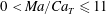 $0<Ma/Ca_{T}\leqslant 11$
a maximum correlation is expected for a threshold
$0<Ma/Ca_{T}\leqslant 11$
a maximum correlation is expected for a threshold
 $0<\unicode[STIX]{x1D6FE}_{th}\leqslant 1$
because
$0<\unicode[STIX]{x1D6FE}_{th}\leqslant 1$
because
 $$\begin{eqnarray}\left.\begin{array}{@{}c@{}}\unicode[STIX]{x1D6FE}_{th}=0\Rightarrow \unicode[STIX]{x1D6FC}\equiv 0\\ \unicode[STIX]{x1D6FE}_{th}=1+\unicode[STIX]{x1D700}\Rightarrow \unicode[STIX]{x1D6FC}\equiv 1\end{array}\right\}\Rightarrow \unicode[STIX]{x1D70C}(k_{L},\unicode[STIX]{x1D6FC})=0,\end{eqnarray}$$
(where
 $\unicode[STIX]{x1D700}>0$
is small). Further investigations have shown that for all cases in table 2 this maximum indeed exists and is reached for a threshold
$\unicode[STIX]{x1D700}>0$
is small). Further investigations have shown that for all cases in table 2 this maximum indeed exists and is reached for a threshold
 $0<\unicode[STIX]{x1D6FE}_{th}<0.2$
. For such small
$0<\unicode[STIX]{x1D6FE}_{th}<0.2$
. For such small
 $\unicode[STIX]{x1D6FE}_{th}$
the surfactant concentration within the identified clean area fraction
$\unicode[STIX]{x1D6FE}_{th}$
the surfactant concentration within the identified clean area fraction
 $\unicode[STIX]{x1D6FC}_{\unicode[STIX]{x1D6FE}_{th}}$
will be very low so that its local contribution to
$\unicode[STIX]{x1D6FC}_{\unicode[STIX]{x1D6FE}_{th}}$
will be very low so that its local contribution to
 $k_{L}$
will be almost identical to the free-slip case (
$k_{L}$
will be almost identical to the free-slip case (
 $Ma/Ca_{T}=0$
). As can be seen in figure 9, assuming a 50-50 split between perfectly clean and extremely dirty areas, the clean area’s contribution to the overall
$Ma/Ca_{T}=0$
). As can be seen in figure 9, assuming a 50-50 split between perfectly clean and extremely dirty areas, the clean area’s contribution to the overall
 $K_{L}$
at
$K_{L}$
at
 $Sc=32$
will be 2.75 times larger than the dirty area’s contribution.
$Sc=32$
will be 2.75 times larger than the dirty area’s contribution.

Figure 14. Time series of clean surface fraction
 $\unicode[STIX]{x1D6FC}$
(a), the corresponding
$\unicode[STIX]{x1D6FC}$
(a), the corresponding
 $k_{L}$
(b) and
$k_{L}$
(b) and
 $-q$
(c) evaluated using the horizontally averaged instantaneous concentration profile from run S2.
$-q$
(c) evaluated using the horizontally averaged instantaneous concentration profile from run S2.
Table 2. Correlation coefficients at
 $Sc=32$
for various thresholds.
$Sc=32$
for various thresholds.

Additionally to the time evolution of
 $\unicode[STIX]{x1D6FC}$
and
$\unicode[STIX]{x1D6FC}$
and
 $k_{L}$
– obtained using (4.5) – figure 14(c) also shows the evolution of the exponent
$k_{L}$
– obtained using (4.5) – figure 14(c) also shows the evolution of the exponent
 $-q$
in the instantaneous power law dependency
$-q$
in the instantaneous power law dependency
 $k_{L}\propto Sc^{-q}$
. In each
$k_{L}\propto Sc^{-q}$
. In each
 $Ma/Ca_{T}$
case, transport equations for five different
$Ma/Ca_{T}$
case, transport equations for five different
 $Sc$
were solved simultaneously – i.e. with exactly the same turbulent flow-field – allowing an unbiased determination of the instantaneous exponent
$Sc$
were solved simultaneously – i.e. with exactly the same turbulent flow-field – allowing an unbiased determination of the instantaneous exponent
 $-q$
using the least squares method. By comparing the temporal evolution of
$-q$
using the least squares method. By comparing the temporal evolution of
 $-q$
and
$-q$
and
 $\unicode[STIX]{x1D6FC}$
, it can be seen that when
$\unicode[STIX]{x1D6FC}$
, it can be seen that when
 $\unicode[STIX]{x1D6FC}$
reduces
$\unicode[STIX]{x1D6FC}$
reduces
 $q$
becomes larger and moves in the direction of
$q$
becomes larger and moves in the direction of
 $2/3$
, which is valid for severe contamination levels. Also, when
$2/3$
, which is valid for severe contamination levels. Also, when
 $\unicode[STIX]{x1D6FC}$
increases,
$\unicode[STIX]{x1D6FC}$
increases,
 $q$
decreases and moves towards
$q$
decreases and moves towards
 $1/2$
, which is valid for clean surface conditions.
$1/2$
, which is valid for clean surface conditions.
The above observations support the idea presented in § 3 of estimating the mean
 $K_{L}$
using the average clean surface fraction
$K_{L}$
using the average clean surface fraction
 $\overline{\unicode[STIX]{x1D6FC}}$
.
$\overline{\unicode[STIX]{x1D6FC}}$
.
4.4 Comparison between observed mean
$q$
,
$c$
and
$K_{L}$
with their predictions based on
$\overline{\unicode[STIX]{x1D6FC}}$


In § 4.3 a good temporal correlation between
 $\unicode[STIX]{x1D6FC}_{0.1}$
and
$\unicode[STIX]{x1D6FC}_{0.1}$
and
 $k_{L}$
for S1 to S3 was obtained. This does not necessarily imply that by using
$k_{L}$
for S1 to S3 was obtained. This does not necessarily imply that by using
 $\unicode[STIX]{x1D6FE}_{th}=0.1$
to determine
$\unicode[STIX]{x1D6FE}_{th}=0.1$
to determine
 $\overline{\unicode[STIX]{x1D6FC}}$
, the prediction of the magnitude of the normalised transfer velocity
$\overline{\unicode[STIX]{x1D6FC}}$
, the prediction of the magnitude of the normalised transfer velocity
 $$\begin{eqnarray}\frac{K_{L}}{u_{\infty }R_{T}^{-1/2}}(\overline{\unicode[STIX]{x1D6FC}})=c(\overline{\unicode[STIX]{x1D6FC}})Sc^{-q(\overline{\unicode[STIX]{x1D6FC}})},\end{eqnarray}$$
where
 $c=c(\overline{\unicode[STIX]{x1D6FC}})$
and
$c=c(\overline{\unicode[STIX]{x1D6FC}})$
and
 $q=q(\overline{\unicode[STIX]{x1D6FC}})$
are determined as in (3.6)–(3.8), is correct. This will be further investigated below.
$q=q(\overline{\unicode[STIX]{x1D6FC}})$
are determined as in (3.6)–(3.8), is correct. This will be further investigated below.
From our results it is possible to directly determine
 $q$
and
$q$
and
 $c$
for each
$c$
for each
 $Ma/Ca_{T}$
case using the least squares method. In figure 10 it is observed that
$Ma/Ca_{T}$
case using the least squares method. In figure 10 it is observed that
 $q$
– corresponding to the gradients of the lines in the log–log plot – varies with
$q$
– corresponding to the gradients of the lines in the log–log plot – varies with
 $Ma/Ca_{T}$
. This relation is investigated further in figure 15(a), which shows an overall smooth variation of
$Ma/Ca_{T}$
. This relation is investigated further in figure 15(a), which shows an overall smooth variation of
 $-q$
from
$-q$
from
 $-1/2$
to
$-1/2$
to
 $-2/3$
with increasing
$-2/3$
with increasing
 $Ma/Ca_{T}$
. Similarly, as seen in figure 15(b), the constant of proportionality
$Ma/Ca_{T}$
. Similarly, as seen in figure 15(b), the constant of proportionality
 $c$
is also found to smoothly vary between its free-slip value
$c$
is also found to smoothly vary between its free-slip value
 $c_{f}$
and its no-slip value
$c_{f}$
and its no-slip value
 $c_{n}$
.
$c_{n}$
.

Figure 15. Variation of (a) exponent
 $-q$
and (b) constant
$-q$
and (b) constant
 $c$
with
$c$
with
 $Ma/Ca_{T}$
. Note results are averaged from
$Ma/Ca_{T}$
. Note results are averaged from
 $t=150{-}300$
and the least-squares method was used to extract
$t=150{-}300$
and the least-squares method was used to extract
 $-q$
and
$-q$
and
 $c$
from the numerical results.
$c$
from the numerical results.
Comparing the results shown in figures 9(a), 13 and 15, a strong correlation can be observed between
 $\overline{\unicode[STIX]{x1D6FC}}$
and each of the time-averaged values
$\overline{\unicode[STIX]{x1D6FC}}$
and each of the time-averaged values
 $q$
,
$q$
,
 $c$
and
$c$
and
 $K_{L}$
. This indicates that in our simulations (where
$K_{L}$
. This indicates that in our simulations (where
 $R_{T}$
and
$R_{T}$
and
 $u_{\infty }$
are approximately the same)
$u_{\infty }$
are approximately the same)
 $K_{L}=cSc^{-q}$
can be modelled as a function of
$K_{L}=cSc^{-q}$
can be modelled as a function of
 $\overline{\unicode[STIX]{x1D6FC}}$
alone.
$\overline{\unicode[STIX]{x1D6FC}}$
alone.
To determine the surfactant-free fraction
 $\overline{\unicode[STIX]{x1D6FC}}$
in (3.6) and (3.8) from the numerical results, we need to determine the optimum threshold
$\overline{\unicode[STIX]{x1D6FC}}$
in (3.6) and (3.8) from the numerical results, we need to determine the optimum threshold
 $\unicode[STIX]{x1D6FE}_{th}$
in (4.6) so that the sum of the squared errors
$\unicode[STIX]{x1D6FE}_{th}$
in (4.6) so that the sum of the squared errors
 $$\begin{eqnarray}SSE(\overline{\unicode[STIX]{x1D6FC}_{\unicode[STIX]{x1D6FE}_{th}}})=\mathop{\sum }_{S0}^{SN}[K_{L}-K_{L}(\overline{\unicode[STIX]{x1D6FC}_{\unicode[STIX]{x1D6FE}_{th}}})]^{2}\end{eqnarray}$$
is minimum, where
 $K_{L}$
is the reference value directly obtained from the numerical results and
$K_{L}$
is the reference value directly obtained from the numerical results and
 $K_{L}(\overline{\unicode[STIX]{x1D6FC}_{\unicode[STIX]{x1D6FE}_{th}}})$
is the predicted transfer velocity calculated using (3.6), (3.8) and (1.6). The parameters
$K_{L}(\overline{\unicode[STIX]{x1D6FC}_{\unicode[STIX]{x1D6FE}_{th}}})$
is the predicted transfer velocity calculated using (3.6), (3.8) and (1.6). The parameters
 $c_{f}=1.55$
(1.6 in Herlina & Wissink Reference Herlina and Wissink2014) and
$c_{f}=1.55$
(1.6 in Herlina & Wissink Reference Herlina and Wissink2014) and
 $c_{n}=0.94$
(0.95 in Herlina & Wissink Reference Herlina and Wissink2016) are determined from the results of runs S0 (free slip) and SN (no slip), respectively. Note that
$c_{n}=0.94$
(0.95 in Herlina & Wissink Reference Herlina and Wissink2016) are determined from the results of runs S0 (free slip) and SN (no slip), respectively. Note that
 $c_{f}$
and
$c_{f}$
and
 $c_{n}$
may vary depending on the location where
$c_{n}$
may vary depending on the location where
 $u_{\infty }$
and
$u_{\infty }$
and
 $L_{\infty }$
are evaluated (see also § 4.1). Since our simulations fall into the low to moderate turbulence intensity regime, we assume that
$L_{\infty }$
are evaluated (see also § 4.1). Since our simulations fall into the low to moderate turbulence intensity regime, we assume that
 $r=1/2$
in (1.6).
$r=1/2$
in (1.6).
As shown in figure 16 the
 $SSE$
obtained using
$SSE$
obtained using
 $\unicode[STIX]{x1D6FE}_{th}=0.1,\ldots ,0.5$
reaches a minimum between
$\unicode[STIX]{x1D6FE}_{th}=0.1,\ldots ,0.5$
reaches a minimum between
 $\unicode[STIX]{x1D6FE}_{th}=0.4$
and 0.5. Despite the good temporal correlations between
$\unicode[STIX]{x1D6FE}_{th}=0.4$
and 0.5. Despite the good temporal correlations between
 $\unicode[STIX]{x1D6FC}$
and
$\unicode[STIX]{x1D6FC}$
and
 $k_{L}$
obtained for smaller
$k_{L}$
obtained for smaller
 $\unicode[STIX]{x1D6FE}_{th}$
, figure 16 shows that by using such small
$\unicode[STIX]{x1D6FE}_{th}$
, figure 16 shows that by using such small
 $\unicode[STIX]{x1D6FE}_{th}$
to determine
$\unicode[STIX]{x1D6FE}_{th}$
to determine
 $\overline{\unicode[STIX]{x1D6FC}}$
the actual magnitude of
$\overline{\unicode[STIX]{x1D6FC}}$
the actual magnitude of
 $K_{L}=\overline{k_{L}}$
is significantly underestimated. Unless specified differently, a threshold of
$K_{L}=\overline{k_{L}}$
is significantly underestimated. Unless specified differently, a threshold of
 $\unicode[STIX]{x1D6FE}_{th}=0.45$
was used for the determination of
$\unicode[STIX]{x1D6FE}_{th}=0.45$
was used for the determination of
 $\overline{\unicode[STIX]{x1D6FC}}$
below.
$\overline{\unicode[STIX]{x1D6FC}}$
below.

Figure 16. Sum of squared errors defined in (4.10).
To test the quality of our prediction of
 $q$
and
$q$
and
 $c$
using
$c$
using
 $\overline{\unicode[STIX]{x1D6FC}_{0.45}}$
, in figure 15 the predicted data points are shown alongside the numerical results, showing a reasonable agreement. In addition, the dashed line, which was produced using the exponential relationship (4.7) between
$\overline{\unicode[STIX]{x1D6FC}_{0.45}}$
, in figure 15 the predicted data points are shown alongside the numerical results, showing a reasonable agreement. In addition, the dashed line, which was produced using the exponential relationship (4.7) between
 $Ma/Ca_{T}$
and
$Ma/Ca_{T}$
and
 $\overline{\unicode[STIX]{x1D6FC}_{0.45}}$
, can be seen to provide a nice interpolation between the data points.
$\overline{\unicode[STIX]{x1D6FC}_{0.45}}$
, can be seen to provide a nice interpolation between the data points.
Finally, based on the reasonably good prediction achieved above for
 $q$
and
$q$
and
 $c$
, it is expected that the proposed model based on the clean surface fraction also provides a prediction of at least similar quality for the transfer velocity. This is indeed confirmed in figure 17, illustrating that the calculation of the normalised transfer velocity from (4.9) both (i) directly by employing the observed
$c$
, it is expected that the proposed model based on the clean surface fraction also provides a prediction of at least similar quality for the transfer velocity. This is indeed confirmed in figure 17, illustrating that the calculation of the normalised transfer velocity from (4.9) both (i) directly by employing the observed
 $\overline{\unicode[STIX]{x1D6FC}_{0.45}}$
 $$\begin{eqnarray}\frac{K_{L}}{u_{\infty }R_{T}^{-1/2}}(\overline{\unicode[STIX]{x1D6FC}_{0.45}})\end{eqnarray}$$
and (ii) indirectly by using (4.7) where
 $\overline{\unicode[STIX]{x1D6FC}_{0.45}}$
is estimated as a function of
$\overline{\unicode[STIX]{x1D6FC}_{0.45}}$
is estimated as a function of
 $Ma/Ca_{T}$
 $$\begin{eqnarray}\frac{K_{L}}{u_{\infty }R_{T}^{-1/2}}(Ma/Ca_{T})=\frac{K_{L}}{u_{\infty }R_{T}^{-1/2}}(\overline{\unicode[STIX]{x1D6FC}_{0.45}}(Ma/Ca_{T}))\end{eqnarray}$$
agree well with the normalised transfer velocity
 $K_{L}$
that was directly obtained from the numerical data. Especially, the initially steep decline in
$K_{L}$
that was directly obtained from the numerical data. Especially, the initially steep decline in
 $K_{L}$
for small
$K_{L}$
for small
 $Ma/Ca_{T}$
is well captured with a maximum error of 8 %. Also, for larger
$Ma/Ca_{T}$
is well captured with a maximum error of 8 %. Also, for larger
 $Ma/Ca_{T}$
a smooth transition to severely contaminated conditions is predicted.
$Ma/Ca_{T}$
a smooth transition to severely contaminated conditions is predicted.

Figure 17. Comparison of the predicted
 $K_{L}$
with present numerical results as a function of
$K_{L}$
with present numerical results as a function of
 $Ma/Ca_{T}$
. (a) Results obtained for
$Ma/Ca_{T}$
. (a) Results obtained for
 $Sc=2$
, 8, 32, (b) close up of
$Sc=2$
, 8, 32, (b) close up of
 $Sc=32$
results for low to moderate
$Sc=32$
results for low to moderate
 $Ma/Ca_{T}$
.
$Ma/Ca_{T}$
.
5 Conclusions
In order to study the influence of surfactants on interfacial mass transfer, direct numerical simulations with various levels of contamination have been performed. At the surface of the computational domain the waves are assumed to be very shallow so that a rigid lid assumption can be employed. In all simulations, mass transfer – promoted by introducing isotropic turbulence at the bottom of the computational domain – is calculated simultaneously for five different Schmidt numbers,
 $Sc=2$
, 4, 8, 16, 32. At the bottom of all simulations the same turbulent flow field is introduced. Consequently, both the turbulent Reynolds numbers and integral length scales are kept within a small range of
$Sc=2$
, 4, 8, 16, 32. At the bottom of all simulations the same turbulent flow field is introduced. Consequently, both the turbulent Reynolds numbers and integral length scales are kept within a small range of
 $R_{T}=129\pm 12$
and
$R_{T}=129\pm 12$
and
 $L_{\infty }=0.96\pm 0.08$
, which allows for the first time an unbiased study of the effect of
$L_{\infty }=0.96\pm 0.08$
, which allows for the first time an unbiased study of the effect of
 $Ma/Ca_{T}$
on
$Ma/Ca_{T}$
on
 $Sc$
. In the surface plane, an advection-diffusion equation is solved for the surfactant concentration. The model described in Shen et al. (Reference Shen, Yue and Triantafyllou2004) is adopted to account for the influence of gradients in the surfactant concentration on the near-surface turbulent flow field, which in turn affects the interfacial mass transfer. The ratio of the Marangoni number and the turbulent capillary number,
$Sc$
. In the surface plane, an advection-diffusion equation is solved for the surfactant concentration. The model described in Shen et al. (Reference Shen, Yue and Triantafyllou2004) is adopted to account for the influence of gradients in the surfactant concentration on the near-surface turbulent flow field, which in turn affects the interfacial mass transfer. The ratio of the Marangoni number and the turbulent capillary number,
 $Ma/Ca_{T}$
, is used as a measure of contamination.
$Ma/Ca_{T}$
, is used as a measure of contamination.
In our previous simulations we investigated interfacial mass transfer for a range of
 $R_{T}$
and
$R_{T}$
and
 $Sc$
up to 500 using either a free-slip boundary condition at the surface (Herlina & Wissink Reference Herlina and Wissink2014) or a no-slip boundary condition (Herlina & Wissink Reference Herlina and Wissink2016). The power dependency of
$Sc$
up to 500 using either a free-slip boundary condition at the surface (Herlina & Wissink Reference Herlina and Wissink2014) or a no-slip boundary condition (Herlina & Wissink Reference Herlina and Wissink2016). The power dependency of
 $K_{L}$
on
$K_{L}$
on
 $R_{T}$
was found to be independent on the surface boundary conditions. For the range of
$R_{T}$
was found to be independent on the surface boundary conditions. For the range of
 $R_{T}$
considered, it was shown that
$R_{T}$
considered, it was shown that
 $K_{L}\propto R_{T}^{-1/2}$
for
$K_{L}\propto R_{T}^{-1/2}$
for
 $R_{T}<R_{T,crit}$
and
$R_{T}<R_{T,crit}$
and
 $K_{L}\propto R_{T}^{-1/4}$
for
$K_{L}\propto R_{T}^{-1/4}$
for
 $R_{T}>R_{T,crit}$
, where
$R_{T}>R_{T,crit}$
, where
 $R_{T,crit}\approx 500$
. This suggests that the same power dependency of
$R_{T,crit}\approx 500$
. This suggests that the same power dependency of
 $K_{L}$
on
$K_{L}$
on
 $R_{T}$
is also likely to be valid for any level of contamination. Hence, as in the present simulations
$R_{T}$
is also likely to be valid for any level of contamination. Hence, as in the present simulations
 $R_{T}<R_{T,crit}$
, the transfer velocity is normalised using
$R_{T}<R_{T,crit}$
, the transfer velocity is normalised using
 $R_{T}^{-1/2}u_{\infty }$
. On the other hand, for the entire range of
$R_{T}^{-1/2}u_{\infty }$
. On the other hand, for the entire range of
 $Sc$
investigated in our previous simulations it was confirmed that the transfer velocity scales with
$Sc$
investigated in our previous simulations it was confirmed that the transfer velocity scales with
 $Sc^{-1/2}$
and
$Sc^{-1/2}$
and
 $Sc^{-2/3}$
for the free-slip and no-slip cases, respectively.
$Sc^{-2/3}$
for the free-slip and no-slip cases, respectively.
In the present DNS, it is found that even small levels of contamination significantly affect the near-surface turbulence so that
 $K_{L}$
no longer scales with
$K_{L}$
no longer scales with
 $Sc^{-1/2}$
. In the no-slip case the surface divergence is strictly zero, which significantly reduces the interchange of saturated and unsaturated fluid. Because of the nearly zero surface divergence, a similar reduction in gas exchange can also be expected in cases with large
$Sc^{-1/2}$
. In the no-slip case the surface divergence is strictly zero, which significantly reduces the interchange of saturated and unsaturated fluid. Because of the nearly zero surface divergence, a similar reduction in gas exchange can also be expected in cases with large
 $Ma/Ca_{T}$
. So even though the near surface hydrodynamics of highly contaminated surfaces (
$Ma/Ca_{T}$
. So even though the near surface hydrodynamics of highly contaminated surfaces (
 $Ma/Ca_{T}\rightarrow \infty$
) does not entirely converge to the no-slip case, the scaling of the transfer velocity becomes similar, i.e.
$Ma/Ca_{T}\rightarrow \infty$
) does not entirely converge to the no-slip case, the scaling of the transfer velocity becomes similar, i.e.
 $K_{L}\propto Sc^{-2/3}$
. For intermediate levels of contamination,
$K_{L}\propto Sc^{-2/3}$
. For intermediate levels of contamination,
 $K_{L}$
is found to approximately scale with
$K_{L}$
is found to approximately scale with
 $Sc^{-q}$
, where
$Sc^{-q}$
, where
 $q$
is shown to gradually increase from
$q$
is shown to gradually increase from
 $1/2$
to
$1/2$
to
 $2/3$
with increasing levels of contamination. Consequently, the surface divergence model, which assumes that
$2/3$
with increasing levels of contamination. Consequently, the surface divergence model, which assumes that
 $K_{L}\propto Sc^{-1/2}$
, is no longer accurate in the presence of even slight contamination.
$K_{L}\propto Sc^{-1/2}$
, is no longer accurate in the presence of even slight contamination.
It is shown that Marangoni forces generate instantaneous shear at the surface which for small to moderate
 $Ma/Ca_{T}$
tends to increase with contamination level. For large
$Ma/Ca_{T}$
tends to increase with contamination level. For large
 $Ma/Ca_{T}$
the surface flow field becomes virtually divergence free, even though, compared to the no-slip boundary condition, a non-zero 2-D flow field persists.
$Ma/Ca_{T}$
the surface flow field becomes virtually divergence free, even though, compared to the no-slip boundary condition, a non-zero 2-D flow field persists.
For small
 $Ma/Ca_{T}$
, regions with very low surfactant concentration are found to appear, which are observed to gradually reduce in size with increasing
$Ma/Ca_{T}$
, regions with very low surfactant concentration are found to appear, which are observed to gradually reduce in size with increasing
 $Ma/Ca_{T}$
. The fraction of the surface that these clean regions occupy is represented by the parameter
$Ma/Ca_{T}$
. The fraction of the surface that these clean regions occupy is represented by the parameter
 $0\leqslant \unicode[STIX]{x1D6FC}\leqslant 1$
. For constant
$0\leqslant \unicode[STIX]{x1D6FC}\leqslant 1$
. For constant
 $Sc$
and
$Sc$
and
 $R_{T}$
the transfer velocity is found to correlate very well with the clean surface fraction, suggesting that
$R_{T}$
the transfer velocity is found to correlate very well with the clean surface fraction, suggesting that
 $K_{L}$
can be regarded as a function of
$K_{L}$
can be regarded as a function of
 $R_{T}$
,
$R_{T}$
,
 $Sc$
and
$Sc$
and
 $\unicode[STIX]{x1D6FC}$
. By assuming that the ‘clean’ regions behave as a free-slip boundary, while the remaining ‘dirty’ regions behave as a no-slip boundary, a model for the transfer velocity that accounts for the presence of surfactants is obtained:
$\unicode[STIX]{x1D6FC}$
. By assuming that the ‘clean’ regions behave as a free-slip boundary, while the remaining ‘dirty’ regions behave as a no-slip boundary, a model for the transfer velocity that accounts for the presence of surfactants is obtained:
 $$\begin{eqnarray}K_{L}=cu_{\infty }Sc^{-q}R_{T}^{-r},\end{eqnarray}$$
with
 $$\begin{eqnarray}\left.\begin{array}{@{}c@{}}c=\overline{\unicode[STIX]{x1D6FC}}c_{f}+(1-\overline{\unicode[STIX]{x1D6FC}})c_{n},\\ q={\displaystyle \frac{2}{3}}-{\displaystyle \frac{\overline{\unicode[STIX]{x1D6FC}}c_{f}}{6c}},\end{array}\right\}\end{eqnarray}$$
where
 $c_{f}$
and
$c_{f}$
and
 $c_{n}$
are the constants of proportionality for the free-slip and no-slip cases, respectively, and
$c_{n}$
are the constants of proportionality for the free-slip and no-slip cases, respectively, and
 $r=1/2$
or
$r=1/2$
or
 $1/4$
depending on the turbulence intensity. A reasonably good prediction of the average transfer velocity, with a maximum error of 8 %, is obtained by identifying
$1/4$
depending on the turbulence intensity. A reasonably good prediction of the average transfer velocity, with a maximum error of 8 %, is obtained by identifying
 $\unicode[STIX]{x1D6FC}$
with the average surface fraction where
$\unicode[STIX]{x1D6FC}$
with the average surface fraction where
 $\unicode[STIX]{x1D6FE}/\unicode[STIX]{x1D6FE}_{max}<0.45$
.
$\unicode[STIX]{x1D6FE}/\unicode[STIX]{x1D6FE}_{max}<0.45$
.
The present results confirm that to predict mass transfer accurately, surface contamination effects need to be taken into account. Hence, information is needed of both the turbulent flow characteristics and the concentration distribution of the surfactant. The latter may become possible with further advances in remote sensing technology, which will allow a quantification of the mean clean surface fraction
 $\overline{\unicode[STIX]{x1D6FC}}$
.
$\overline{\unicode[STIX]{x1D6FC}}$
.
Acknowledgements
This research was funded by the German Research Foundation (DFG UH242/6-1). The authors would like to thank the Steinbuch Centre for Computing (SCC) in Karlsruhe for providing computing time on the HP XC 3000. We would also like to thank the anonymous reviewers for their invaluable suggestions for improvement.


